Article

Evaluating the Performance of Photogrammetric Products Using Fixed-Wing UAV Imagery over a Mixed Conifer–Broadleaf Forest: Comparison with Airborne Laser Scanning

1
Department of Global Agricultural Sciences, Graduate School of Agricultural and Life Sciences, The University of Tokyo, Tokyo 113-8657, Japan
2
The University of Tokyo Hokkaido Forest, Graduate School of Agricultural and Life Sciences, The University of Tokyo, Furano, Hokkaido 079-1563, Japan
*
Author to whom correspondence should be addressed.
Remote Sens. 2018, 10(2), 187; https://doi.org/10.3390/rs10020187
Submission received: 21 December 2017 / Revised: 18 January 2018 / Accepted: 25 January 2018 / Published: 27 January 2018
(This article belongs to the Section Forest Remote Sensing)

Abstract

:
Unmanned aerial vehicles (UAVs) and digital photogrammetric techniques are two recent advances in remote sensing (RS) technology that are emerging as alternatives to high-cost airborne laser scanning (ALS) data sources. Despite the potential of UAVs in forestry applications, very few studies have included detailed analyses of UAV photogrammetric products at larger scales or over a range of forest types, including mixed conifer–broadleaf forests. In this study, we assessed the performance of fixed-wing UAV photogrammetric products of a mixed conifer–broadleaf forest with varying levels of canopy structural complexity. We demonstrate that fixed-wing UAVs are capable of efficiently collecting image data at local scales and that UAV imagery can be effectively utilized with digital photogrammetric techniques to provide detailed automated reconstruction of the three-dimensional (3D) canopy surface of mixed conifer–broadleaf forests. When combined with an accurate digital terrain model (DTM), UAV photogrammetric products are promising for producing reliable structural measurements of the forest canopy. However, the performance of UAV photogrammetric products is likely to be influenced by the structural complexity of the forest canopy. Furthermore, we highlight the potential of fixed-wing UAVs in operational forest management at the forest management compartment level, for acquiring high-resolution imagery at low cost. A future direction of this research would be to address the issue of how well the photogrammetric products can predict the actual structure of mixed conifer–broadleaf forests.

Graphical Abstract

1. Introduction

Forest canopy structure has many components but often refers to the size and spatial arrangement of overstory trees as described by the vertical and horizontal distributions of overstory foliage [1,2]. Because of the strong allometric relationship between the forest canopy and other aspects of forest structure, it has been intensively studied as a surrogate for overall forest structure. In addition, the forest canopy plays an important role as a biotic habitat [3], an area of high photosynthetic capacity [4], an indicator of biodiversity [2,5,6], and a gauge of forest health [7]. However, our understanding of forest canopy structure may be constrained in some important ways (e.g., structural and spatial complexity of the canopy at the landscape level) because most existing studies of the forest canopy are based on data collected through field surveys within a small set of sample plots that are often selected subjectively [8,9]. In addition, characterisation of the three-dimensional (3D) structure of the forest canopy using conventional field survey data is challenging because of physical access and resource requirements [10,11].
By providing varying spatial, spectral, and temporal resolution as well as effective means of 3D canopy reconstruction, the use of remote sensing (RS) technology addresses these issues. RS has also proven an effective means of studying forest canopy structure, as it often complements existing ground-based techniques by contributing reliable, detailed information on various aspects of the complex forest canopy [12,13,14]. In particular, recent advances in RS technology, such as airborne laser scanning (ALS), digital photogrammetry, and unmanned aerial vehicle (UAV) systems, have enabled efficient data collection and fully automated reconstruction of forest canopy surfaces over large spatial areas [15,16,17,18,19,20,21,22].
ALS is an active RS technique that uses a light detection and ranging (LiDAR) sensor, which emits a laser beam across the flight path at an operator-specified angle and receives the reflected energy. This technique allows users to determine the distance from the sensor to a target object using either discrete return (pulse ranging) or continuous wave systems. LiDAR measurements have proven to be more successful than other remote sensing options at reconstructing 3D forest canopy structure and more accurate at predicting structural attributes, particularly when acquired with satisfactory point densities [9,16,17]. In addition, this method provides otherwise unavailable scientific insights by allowing for detailed and novel structural measurements [14,23,24]. Therefore, the application of LiDAR measurements to analysing forest canopy structure has been researched intensively in terms of both the area-based approach (ABA) and individual tree-based methods [16,25,26,27,28]. Nonetheless, the main limitations of ALS in practice are the high acquisition cost, which limits its application to operational forest management, and the absence of spectral data that can lead to other important information, such as species identification.
Digital photogrammetric techniques such as structure from motion (SfM) also facilitate 3D modelling of forest canopy structure. Following the principles of traditional stereoscopic photogrammetry, SfM uses multiple images from different angular viewpoints to identify well-defined geometric features and to generate a 3D point cloud [15,29]. Recently, many studies have taken advantage of digital photogrammetry (e.g., [30,31,32,33,34]), particularly for estimating the biophysical properties of individual trees and plot-level forest structural attributes with reasonable accuracy (e.g., [35,36,37,38,39,40]). Moreover, many previous studies attempted to compare photogrammetric products i.e., point clouds, CHMs and structural metrics with LiDAR data [19,39,40,41,42,43,44,45,46,47,48,49]. Recent advances in computer vision algorithms, such as the scale invariant feature transform (SIFT), and parallel bundle adjustments on graphics processing units (GPUs) [15] have enhanced the potential to match image features in many overlapping photographs (100 s–1000 s) acquired from different angles. Thus, SfM can be used effectively to process imagery acquired from UAV platforms (i.e., small multi-rotor or fixed-wing UAVs of less than 5 kg) [21,22,50,51,52].
The UAV system is a newly emerging method of fine-scale remote sensing that has the key advantages of (1) flexibility and decentralization of data acquisition; (2) potential for obtaining data with high spatial and temporal resolution; (3) insensitivity to cloud cover; and (4) low operational costs. High-resolution UAV imagery can be utilized to develop point clouds as well as to extract fundamental characteristics such as tone (color), texture, pattern, shape or association [18,21,22]. Nevertheless, out of those fundamental characteristics, tone and texture can be easily used for digital interpretation of the imagery. Therefore, UAV platforms represent a low-cost remote sensing alternative to airborne and satellite platforms and enable the production of cost-effective data with an unrivalled combination of spatial and temporal resolution at local scales (e.g., for areas the size of traditional forest plots up to the size of forest compartments) [53]. These characteristics have created new possibilities for the utilization of UAV systems and the SfM technique in forest management to collect information on the spatial and structural variability of the forest canopy [18,22,38,45,51].
Currently, three types of small UAV platforms that are widely used for scientific research are available on the market: multi-rotor, single-rotor (similar in design and structure to a helicopter), and fixed-wing UAVs [54]. Single-rotor UAVs (in comparison to multi-rotor UAVs) have the advantage of efficient power consumption but they have limited agility, higher complexity, operational risk and product costs. Compared to multi-rotor UAVs, fixed-wing models are superior in forestry applications because of several factors, including (1) faster flying speeds that allow them to cover large areas without being influenced by wind resistance or bad weather as easily as multi-rotors; (2) long endurance and an extended battery life that enable them to cover many miles in a single session; (3) an ability to carry heavier payloads; and (4) capability to fly at higher altitudes that permit a greater visual line of sight (VLOS) range. Thus, fixed-wing UAVs enable efficient data collection over larger areas and are a viable option for forestry applications, including operational forest management that requires geo-referenced imagery at comparatively large scales.
Although fixed-wing UAVs have great potential for use in forestry applications, very few studies have involved detailed analyses of point clouds or canopy surface models built from fixed-wing UAV imagery at comparatively large scales, such as the forest management compartment level, and even fewer studies have used fixed-wing UAV imagery to estimate forest structural attributes (e.g., [19,38,55]). Applications of fixed-wing UAV imagery and the robustness of digital photogrammetry have also not been studied intensively over a range of forest types, such as mixed conifer–broadleaf forests. In this study, we address these issues.
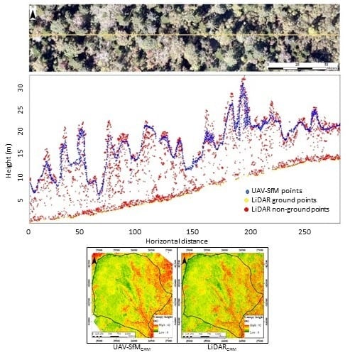
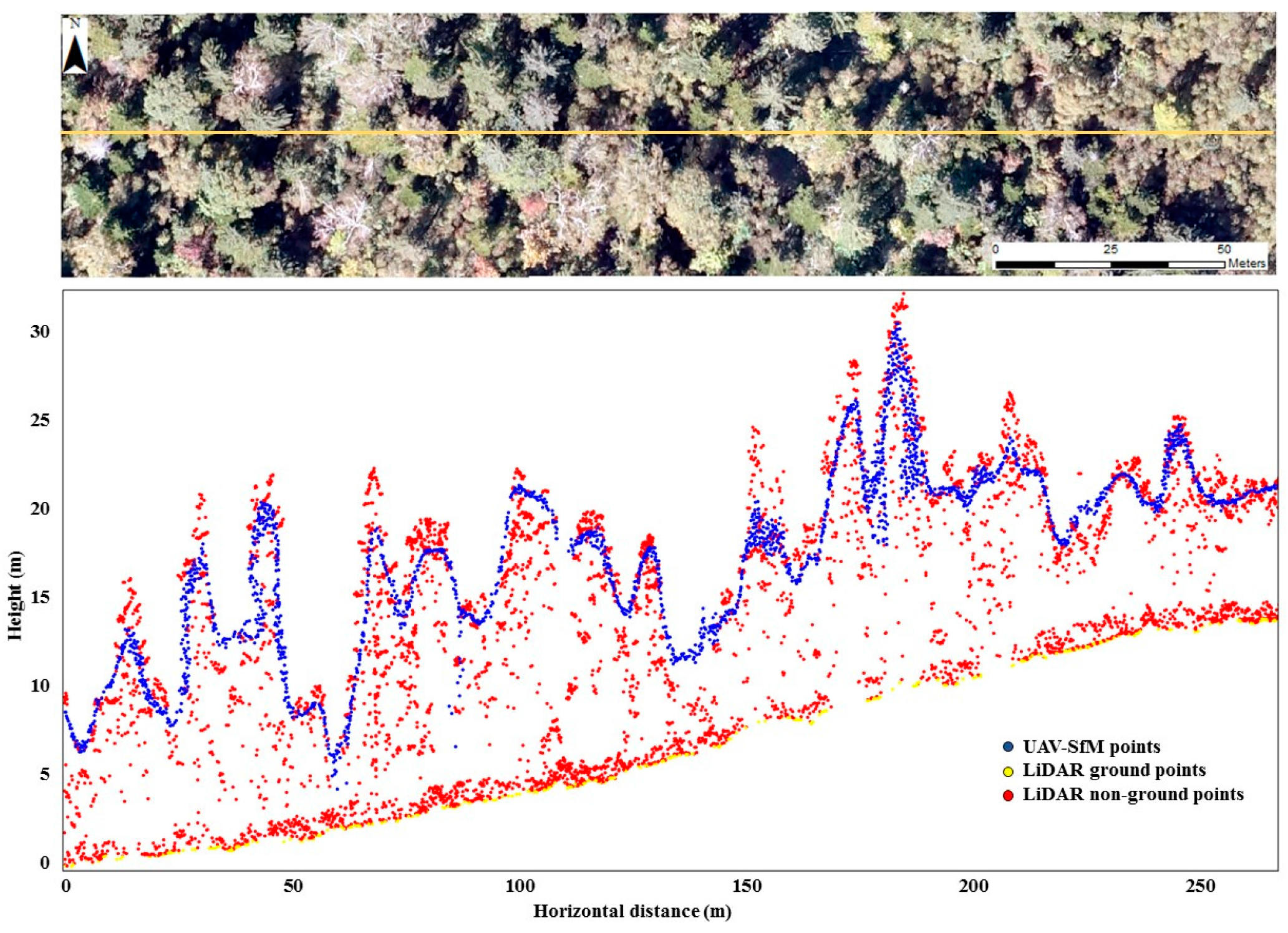
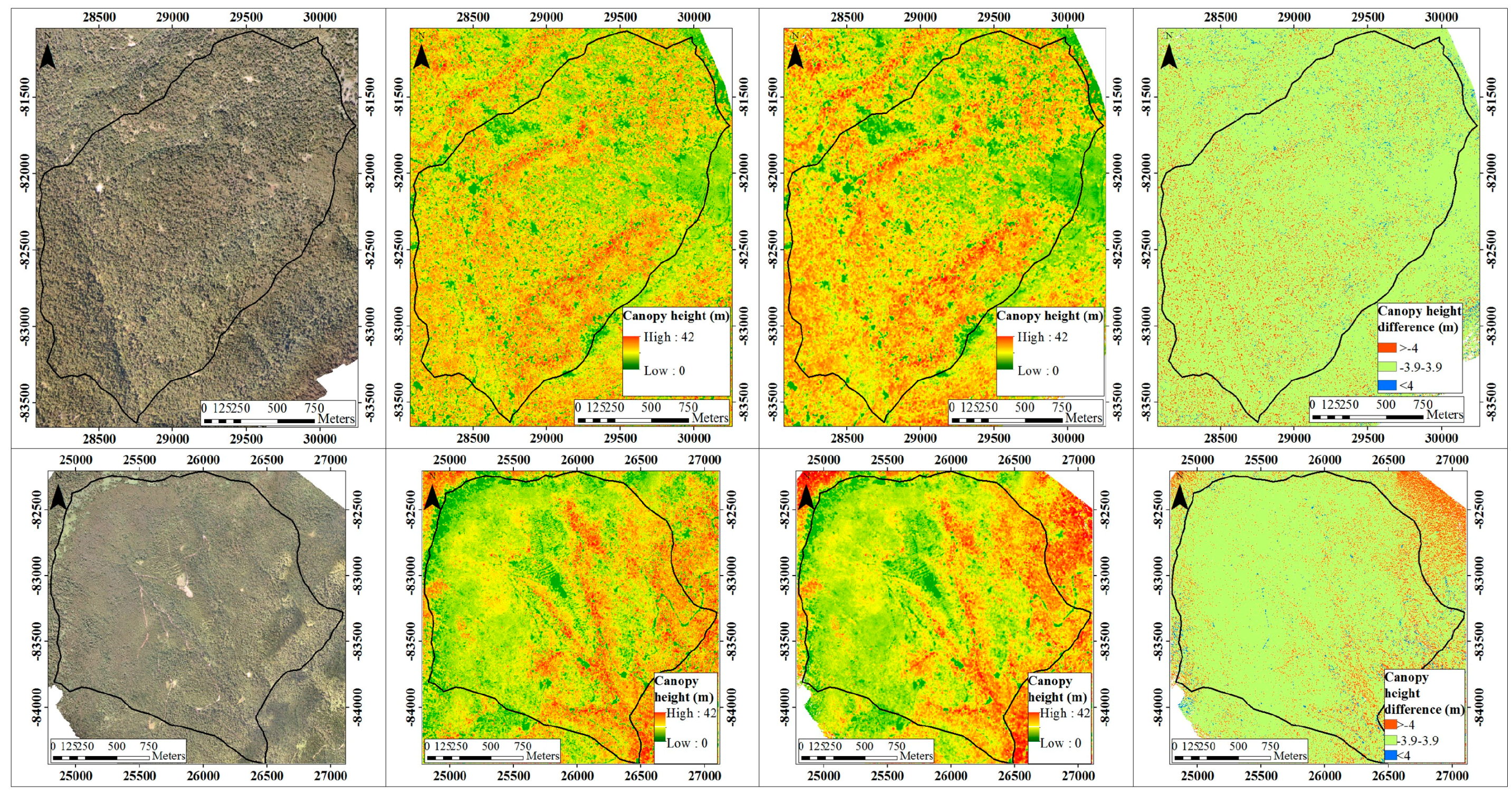
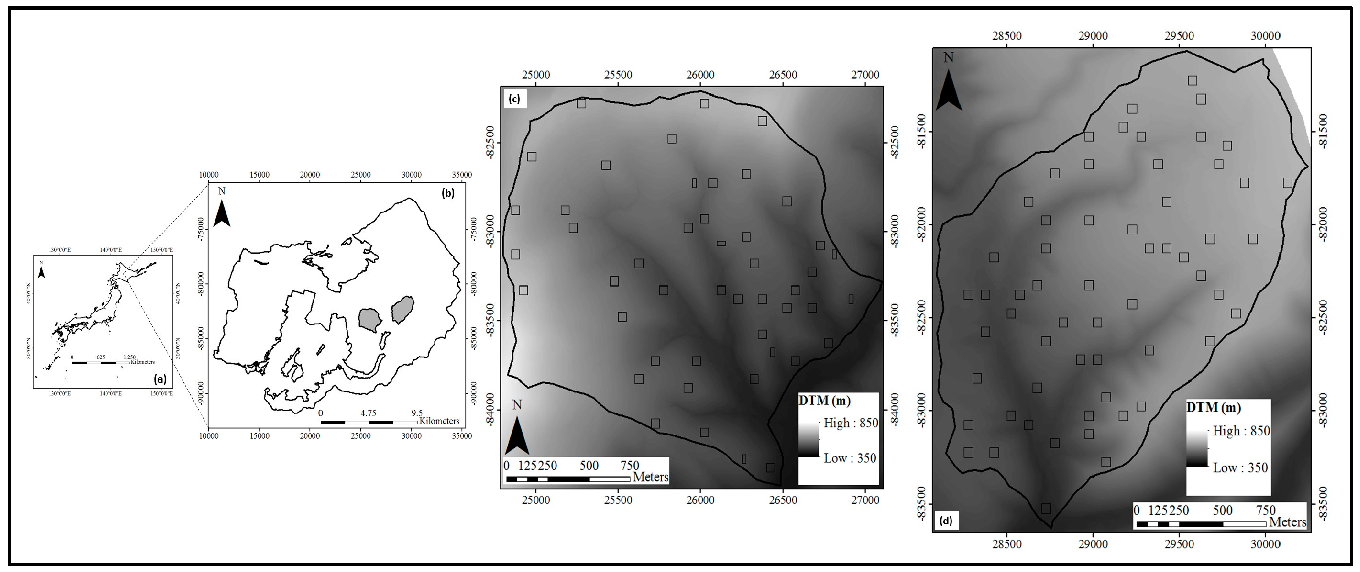
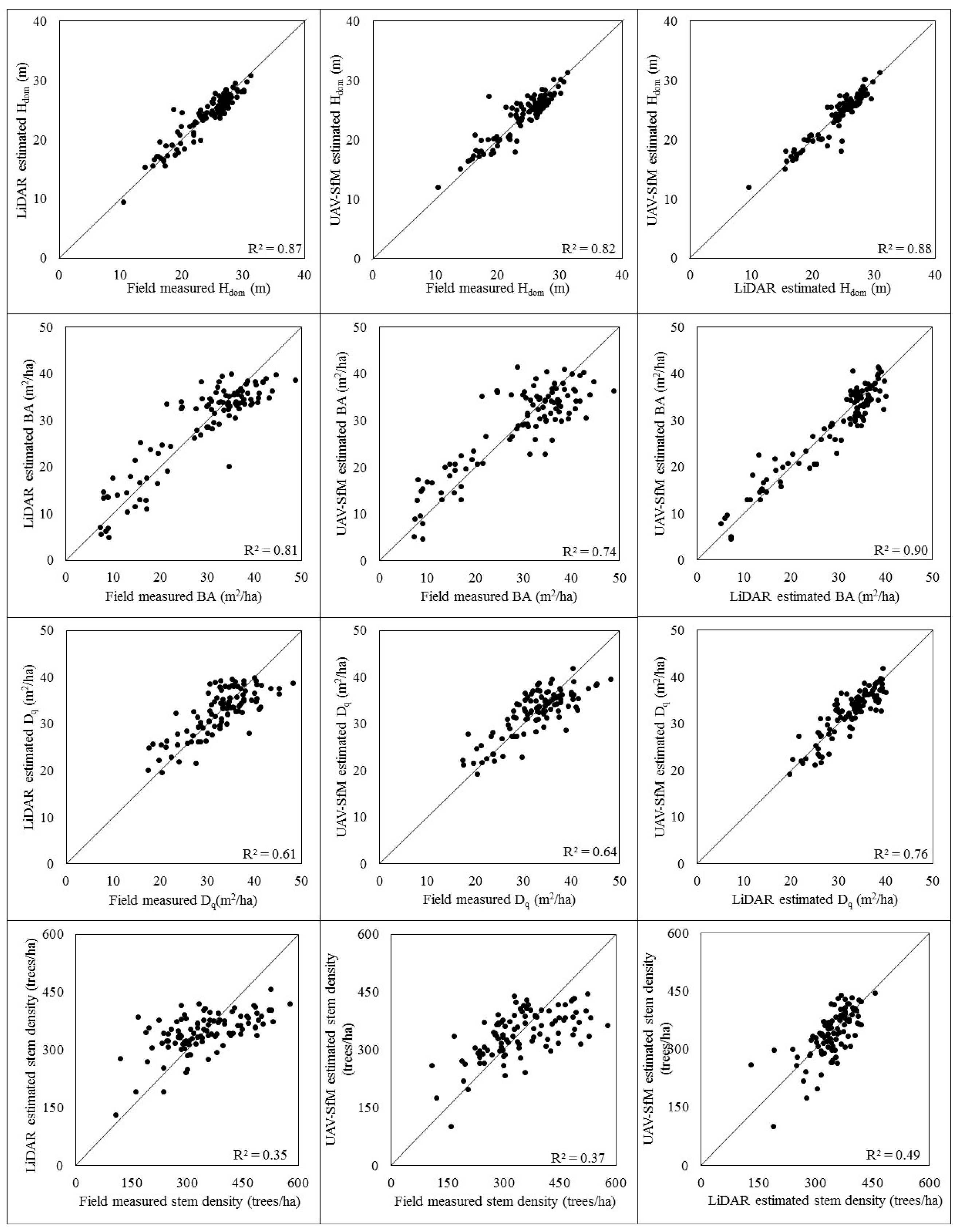
The aim of the present study was to assess the performance of image-based point clouds derived from fixed-wing UAV imagery captured over a mixed conifer–broadleaf forest with varying levels of canopy structural complexity. First, we conducted a detailed evaluation of UAV-SfM outputs by comparing UAV-SfM-derived canopy height models (CHMs) and structural metrics to LiDAR-derived CHMs and structural metrics. We used LiDAR data as a reference data set to assess the performance of UAV-SfM, as they are considered reliable for forestry applications for two main reasons: (1) the non-clustering effect of LiDAR data leads to accurate estimation of forest structural attributes and (2) the data have a proven ability to reconstruct 3D canopy structure with high accuracy for a variety of forest types [40,43,48,
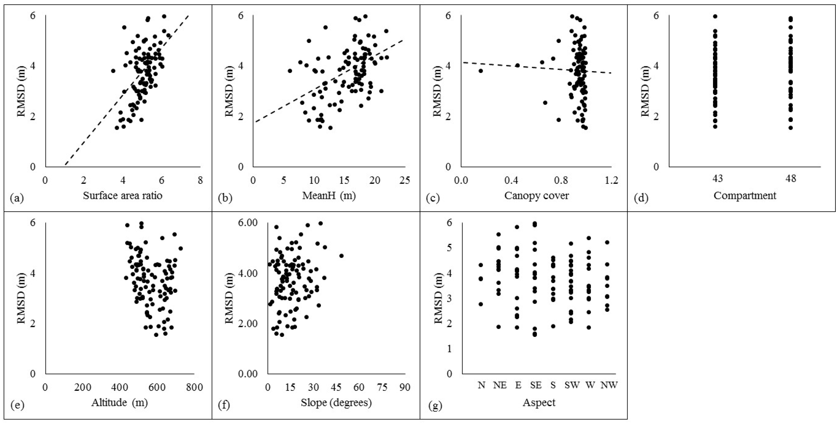
56]. Second, we assessed the utility of UAV-SfM-derived point clouds for estimating several forest structural attributes that are commonly used in forestry applications. Finally, we examined the effects of forest canopy structural metrics and terrain conditions on the performance of the UAV-SfM canopy model.

2. Materials and Methods

2.1. Study Site

This study was carried out in the University of Tokyo (UTokyo) Hokkaido Forest (Figure 1b), where forest management activities such as selection cutting and enrichment planting are practiced. The UTokyo Hokkaido Forest is located in Furano City in the central part of Hokkaido Island in northern Japan (43°10–20′N, 142°18–40′E, 189–1459 m a.s.l.) and has a total area of 22,715 ha. The mean temperature was 6.4 °C and precipitation was 1297 mm at the arboretum (230 m) in 2001–2008. Snow covers the ground from late November to early April, with a maximum depth of about 1 m [57].
The UTokyo Hokkaido Forest is a pan-mixed conifer–broadleaf forest [58] that represents the transition zone between cool-temperate broadleaf forests and subarctic coniferous forests. Abies sachalinensis (Sakhalin fir), one of the dominant tree species in the pan-mixed forest type, grows here at a wide range of elevations (200 to about 1200 m a.s.l.) (200 to about 1200 m a.s.l.; [59]). Other common tree species include Picea jezoensis, P. glehnii, Fraxinus mandshurica, Kalopanax septemlobus, Quercus crispula, Betula maximowicziana, Taxus cuspidata, and Tilia japonica [60]. The forest floor is often occupied by dwarf bamboo (Sasa senanensis and S. kurilensis).
In this study, we intentionally chose two forest management compartments to replicate the UAV flight missions: compartment 43 (Figure 1d) and compartment 48 (Figure 1c), which were scheduled for management in 2016 and 2017, respectively. Part of the forest area in these two compartments is secondary forest recovering from heavy typhoon damage in 1981. Major tree species found in this area include A. sachalinensis, P. jezoensis, Betula ermanii, T. japonica, and P. glehnii. According to forest management planning maps drawn based on field observations, these two compartments consist of several forest stand types, including young broadleaf stands (recovering area), young conifer stands, mixed stands dominated by conifers, mixed stands dominated by broadleaves, and reserve forest area where no management activities are being practiced. No major disturbances were observed in the study area between 2015 and 2017.

2.2. Data Collection

2.2.1. Field Data

A field survey of 105 sample plots representing the major forest stand types (i.e., young broadleaf stands, young conifer stands, conifer-dominated mixed forest stands, broadleaf-dominated mixed forest stands, and reserve forest area) was carried out in two consecutive years. Specifications of the study area and field sample plots are summarised in Table 1. Diameter at breast height (DBH), species, and height data were collected from eight canopy trees in each sample plot. In addition, we used forest inventory data sets from 2016 and 2017. A description of the forest’s structural characteristics is provided in Table 2.

2.2.2. LiDAR Data

LiDAR data were acquired under leaf-on conditions in September 2015 using an Optec Orion M300 sensor (Teledyne Technologies, Waterloo, ON, Canada) mounted on a helicopter. Specifications of LiDAR data are summarised in Table 3. The Optec Orion M300 sensor is capable of capturing up to four range measurements, including first, second, third, and last returns, but in this study we used single, first of many, and last of many returns to represent the ground and canopy signals. Initial processing of LiDAR data was conducted by the data provider (Hokkaido Aero Asahi, Hokkaido, Japan), including classification of points into ground and non-ground classes using TerraScan software (2000–2016 Arttu Soininen, Terrasolid, Helsinki, Finland), and the data were delivered in LAS format (Coordinate system: JGD2000 Japan-19 zone XII/ GSIGEO 2000 geoid).

2.2.3. UAV Imagery

UAV Equipment and Payload

UAV imagery was collected on 17 and 18 September 2015 for compartment 43 and on 2 September 2016 for compartment 48. Images were acquired using a Trimble UX5 (Trimble Navigation, Sunnyvale, CA, USA) small fixed-wing UAV platform that weighs about 2.5 kg with its payload and that was equipped with a lithium-polymer electric battery allowing for a maximum flight time of ~50 min. The UAV was equipped with an on-board global navigation satellite system (GNSS) to provide rough positioning. For this study, the UX5 was equipped with a Sony NEX-5T 16.1 megapixel RGB camera (Sony, Tokyo, Japan) with an APS-C 23.5 × 15.6 mm CMOS image sensor as the payload. The camera weighs approximately 218 g (110.8 × 58.8 × 32.5 mm) and has a shutter speed of 1/4000 s, a focal length of 15 mm, and an ISO that adapts to the light conditions of each shot. These camera settings ensured optimal exposure and prevented images from being affected by motion. Based on the weather condition of the image acquisition days, the actual shutter speed of the camera was changed between 1/1600 s and 1/2000 s.

UAV Imagery Collection: Planning and Implementation

Image acquisition was composed of three phases: the planning phase, the field phase, and flight missions. In the planning phase, we used a flight simulation software package to obtain a plan for flight implementation. The main input parameters required in the planning phase were flight altitude, working area radius, and image overlap. Flight altitude and longitudinal and lateral overlaps were set to 500 m, 95%, and 80%, respectively. However, the defined nominal longitudinal overlap was only indicative, as it was subjected to changes during actual flight because of wind and differences between the simulated and actual flight paths (average flight altitude for compartment 43 was 496 m, while for compartment 48 it was 537 m). The home points (take-off and landing points) and 18 ground control points (GCPs) were located in available open areas.
The field phase included marking GCPs on the ground and measuring their positions. We used 50 × 50 cm targets with a black-and-white checkerboard pattern as GCPs to ensure the greatest possible contrast in the images. After fixing the GCP targets to the ground, we determined their centre position using GPS and GLONASS. The nearest official reference point was used as the base station. Later, we post-processed field-recorded coordinates using correction data from the base station.
The weather was stable during the three days of image collection. For each flight, the UAV took off, ascended to the predetermined flight altitude, flew a parallel track course under GPS control, and then automatically returned to and landed at the launch site. The camera was triggered automatically based on the predefined flight plan, and images were stored in jpeg format. After each UAV flight, images were downloaded to a field laptop. Trimming of unwanted photos resulted in a total of 2592 images (with an image resolution of 4912 × 3264 and a ground resolution of 14.1 cm/pixel) that were subsequently used in the SfM processing workflow.

2.3. Data Analysis

2.3.1. Photogrammetric Processing

We used Agisoft PhotoScan Professional Edition 1.3.2 (Agisoft, St. Petersburg, Russia) to generate 3D dense point clouds, as it has proven effective for the production of dense and accurate point clouds over forested areas [38,51]. PhotoScan offers a user-friendly workflow that combines proprietary algorithms based on computer vision SfM and stereo-matching for image alignment and 3D reconstruction [61]. This workflow consists of two stages: image alignment and point cloud densification. To avoid unsatisfactory 3D reconstruction, we selected parameters for each stage based on the results of an initial analysis of a small area via forward sequential selection [35,48,62].
The first stage of processing, image alignment, consists of sparse reconstruction of the 3D geometry by detection and matching of image feature points in overlapping images using SfM techniques. In this stage, we used the highest image matching option, a key point limit of 40,000 and a tie point limit of 4000. Absolute orientation was successful for all 2592 images. A total of 1,209,531 tie points were generated in the initial alignment. However, to optimise the results, we manually edited the sparse point cloud by deleting mislocated points based on three criteria: reprojection error, reconstruction uncertainty, and projection accuracy. This optimisation reduced the final number of tie points to 1,100,760. To allow for more accurate model reconstruction, we then optimised the camera orientation and internal parameters using GCPs. Optimisation was conducted for focal length in the x and y dimensions (fx, fy), principal point coordinates (cx, cy), radial distortion coefficients (k1, k2, k3), and tangential distortion coefficients (p1, p2).
In the second stage of processing, point cloud densification, the software calculates depth information for images and combines all points into a single dense point cloud. To build the dense point cloud, we selected a medium quality that downscaled the image size from the original image by a factor of 8 to avoid excessive processing time. In addition, mild depth filtering was used to remove outliers and reduce noise. The resulting dense point cloud had 93.98 × 10⁶ points (average point density = 5.8 points/m2) and was exported to LAS format (Coordinate system: JGD2000 Japan-19 zone XII/ GSIGEO 2000 geoid) for further processing. PhotoScan was installed on a workstation with an Intel Core i5-4670 CPU (Intel Corp., Santa Clara, CA, USA) at 3.4 GHz, 16 GB RAM, 64-bit OS, and NVIDIA Quadro K2000 GPU. A total processing time of about 36 h of continuous computation was needed to generate the point cloud across the study site.

2.3.2. Generation and Comparison of LiDAR and UAV-SfM CHMs

We generated canopy height models using point cloud data and compared them to LiDAR canopy height models as the first step in assessing accuracy.

Generation of LiDAR Canopy Height

LiDAR non-ground points and their z values were used to derive the LiDAR digital surface model (LiDARDSM) using the maximum z value of the point cloud within a 1 × 1 m grid used as the DSM height for that grid cell. We considered the average tree crown size in the study area and the point density when determining the grid size. A 1 m grid was chosen because it provided meaningful values for canopy height in the study area. We built the LiDAR digital terrain model (LiDARDTM, 1 m pixel resolution) using a triangulated irregular network (TIN) constructed from LiDAR ground points using Delaunay triangulation. Then we calculated the LiDAR canopy height model (LiDARCHM) by subtracting LiDARDTM from LiDARDSM.

Generation of UAV-SfM Canopy Height

We used UAV-SfM points and their z values to derive the UAV-SfM digital surface model (UAV-SfMDSM) following the same procedure as for LiDARDSM generation. No void filling was used to construct more accurate models. Several studies have highlighted the need for a precise DTM to generate an accurate CHM from SfM [19,51,63]. To reconstruct the precise ground terrain using an SfM point cloud, the ground must be visible from multiple locations. However, this is challenging in forest areas with dense canopy cover [39]. Therefore, we used LiDARDTM to normalise absolute heights in this study, such that we subtracted LiDARDTM from UAV-SfMDSM to obtain the UAV-SfM canopy height model (UAV-SfMCHM).

Comparison of LiDARCHM and UAV-SfMCHM

LiDARCHM and SfMCHM were compared both visually and statistically. The differences between the LiDARCHM and SfMCHM results were also evaluated through direct comparisons of pixel values (i.e., subtraction of UAV-SfMCHM from LiDARCHM) for insight into their altimetric differences at the pixel level.

2.3.3. Extraction and Comparison of Forest Structural Metrics

Although forest canopies are multifaceted, they are commonly studied using the dominant characteristics of canopy structure. Previous forestry studies have assessed the accuracy of remote sensing techniques by extracting various structural metrics that play major roles in forest management and other ecological applications [9,14,23,24,39,43,55]. To assess the accuracy of the UAV-SfM point cloud in detail and to thoroughly evaluate the differences between the UAV-SfM and LiDAR point clouds, we used common plot-level structural metrics that can be easily generated from point cloud data. We calculated the metrics described below for each sample plot (n = 105) using normalised LiDAR and UAV-SfM point cloud data.
  • Maximum height (MaxH)
  • Mean height (MeanH)
  • Standard deviation of heights, also known as the rugosity index [24] (SD of H)
  • Coefficient of variation (CV of H)
  • Skewness and Kurtosis
  • Percentile heights of 10%, 25%, 50%, 75% and 95% (P10, P25, P50, P75 and P95)
  • Canopy cover above 2 m height calculated as the proportion of points above 2 m height to the total number of points (d0)
  • Density of points at 1st, 2nd, …, 9th height fractions (d1, d2, …, d9)
  • Canopy cover above mean height calculated as the proportion of points above mean height to the total number of points (dmean)
  • Surface area ratio that is the proportion of 3D canopy surface area to the ground surface area. Also known as “rumple index” [24].
The cloudmetrics function of the FUSION software package (version 3.60) [64] was used to extract plot-level metrics. We computed all metrics using only points with heights greater than 2 m to eliminate ground and understorey (e.g., Sasa spp.) returns.
To enable comparison of LiDAR and UAV-SfM metrics and assess their agreement, we calculated the mean difference (MD), which indicates whether the UAV-SfM metrics are generally greater or smaller than the corresponding LiDAR metric values, and the root mean square deviation (RMSD), which indicates the average difference between metric values and clarifies the magnitude of the differences between LiDAR and UAV-SfM metric values using the equations given below:
M D = i = 1 n ( ( L i D A R ) i ( U A V S f M ) i ) n
R M S D =   i = 1 n ( ( L i D A R ) i ( U A V S f M ) i ) 2 n ,
where n is the number of sample plots, and (LiDAR)i and (UAV­SfM)i are the LiDAR canopy height and UAV-SfM canopy height, respectively.
To assess the degree of association between metric values, we also calculated the Pearson correlation coefficient (R) between LiDAR and UAV-SfM metric values. Finally, the presence or absence of statistically significant differences between metric mean values was tested using paired two-sample t tests.

2.3.4. Evaluation of the Utility of UAV-SfM-Derived Point Cloud Products and Plot-Level Validation of Canopy Height

To evaluate the utility of UAV-SfM-derived point cloud products for estimating plot-level forest structural attributes we used generalised linear model (GLM) analysis. Based on similar published studies, we selected a subset of structural metrics (described in Section 2.3.3) to be used as predictor variables in our models. First plot-level field forest structural attributes, i.e., dominant height (hdom), basal area (BA), quadratic mean DBH (Dq) and stem density (N), and their logarithmic transformations were related to the RS derived structural metrics using regression analysis. Then the stepwise variable selection was carried out, and the final model was selected based on Akaike’s information criterion (AIC). In addition, the selection of predictor variables was penalised for collinearity using the variance inflation factor (VIF). The accuracy of the predictions was validated at the plot level using leave-one-out cross-validation (CV). The root mean square error (RMSE), relative root mean square error (RMSE%), and bias were determined using the following equations:
R M S E = i = 1 n ( y i y ^ i ) 2 n
R M S E % = ( R M S E y ¯ ) × 100
B i a s = i = 1 n y i y ^ i ) n ,
where n is the number of field plots, y i , is the observed value, y ^ i , predicted value and y ¯ is the mean of n observed values.
We used the terms “MD” (Equation (1)) and “RMSD” (Equation (2)) instead of “bias” and “RMSE” when UAV-SfM data is compared to LiDAR data (as the reference data) to avoid the confusion that UAV-SfM data is being compared to reference data but not to field data. When comparison involves the UAV-SfM predictions of forest structural attributes and field data, the terms “bias” (Equation (2)) and “RMSE” (Equations (3) and (4)) were used exclusively.

2.3.5. Identification of Factors that Affect the Performance of UAV-SfMCHM

We examined the effects of canopy structural complexity and topographic conditions on the performance of UAV-SfMCHM, as these factors affect the performance of digital photogrammetry in forested areas [19,39,48,50]. LiDAR structural metrics are strongly correlated with variation in vertical and horizontal forest structure at the stand level and hence explain the structural complexity of the overall forest canopy [9,65]. Therefore, we selected several plot-level LiDAR structural metrics described in the previous section, including mean height, canopy cover greater than 2 m, and surface area ratio, to determine the influence of stand structure on the RMSD of canopy height. We also tested the effects of ground conditions such as elevation, slope (calculated as the maximum rate of change in z value from one cell to its neighbours), and aspect (which identifies the downslope direction of the maximum rate of change in the value of each cell in relation to its neighbours) that were calculated using LiDARDTM. Compartment was also included as an explanatory variable in the modelling, as stand and site conditions were not identical between the two compartments. We performed multivariate data analysis using a GLM with all metrics inputted as fixed components (compartment and aspect were inputted as categorical factors, whereas all other metrics were inputted as numerical values) to test the statistical significance of each factor as it affects the performance of UAV-SfMCHM.

3. Results

3.1. Comparison of LiDAR and UAV-SfM Outputs

3.1.1. LiDAR and UAV-SfM Point Cloud Properties

A transect of the LiDAR and photogrammetric point clouds is shown in Figure 2 for illustration purposes. Unlike LiDAR pulses, which penetrate the forest canopy to better account for small gaps and peaks, the photogrammetric point cloud had limited capacity to reconstruct small gaps and peaks. The number of points that represented the ground was very low in the photogrammetric point cloud and restricted to areas where large gaps were present or where bare earth was clearly visible from the sky.

3.1.2. LiDAR and UAV-SfM CHMs

LiDARCHM, UAV-SfMCHM, and the canopy height difference model for compartments 43 and 48 are shown in Figure 3. LiDARCHM and UAV-SfMCHM generally showed good agreement, which suggests that the overall quality of the reconstruction was consistent.
RMSD and MD for the study area were 3.89 and −0.70 m, respectively. The RMSD value for compartment 43 (3.75 m) was lower than that for compartment 48 (4.01 m). Furthermore, compartment 43 showed a positive mean difference (MD) of 0.03 m, whereas a negative MD of 1.40 m was observed for compartment 48. A histogram comparing CHMs over the study area is shown in Figure 4. Over the entire study area, 43.9%, 66.7%, and 79.7% of the height values were within ±1, ±2, and ±3 m of the corresponding reference point in LIDARCHM, respectively. Overestimations (in comparison to LiDAR data) by greater than 4 m made up 3.7% of the data, whereas underestimations by less than 4 m accounted for 9.3% of the results. The proportion of pixels with no data, mainly because of shadows, was estimated at 0.6% over the study area. Overall, canopy height differences between LiDARCHM and UAV-SfMCHM were within the range of ±4 m for the majority of the area (88.3% for compartment 43, 84.5% for compartment 48, and 86.4% for both compartments).
In-depth visual comparison highlighted several differences, examples of which are shown in Figure 5. First, large positive differences were observed where occlusions were present, such as some isolated tree crowns that were absent from the photogrammetric canopy surface model despite being well represented in the aerial images (Figure 5a). Second, large negative differences in canopy height occurred mainly where the UAV-SfM technique failed to accurately reconstruct small gaps (Figure 5b). Third, the visual quality of the UAV-SfMCHM varied by stand, species, and tree density (Figure 5a,c,d; e.g., mixed stands suffered more from the smoothing effect induced by dense point matching).
Further comparison of LiDARCHM and UAV-SfMCHM at the plot level is shown in Figure 6. Small gaps and tree tops were better represented by LiDARCHM. Crowns were generally wider and less defined in UAV-SfMCHM, as was observed in the comparison of UAV-SfMCHM with LiDARCHM shown in Figure 3. UAV-SfMCHM was overestimated when LiDARCHM values were close to zero (Figure 6d,h).

3.2. Comparison of Structural Metrics Derived from Photogrametric Products

Comparisons of LiDAR and UAV-SfM structural attributes are summarised in Table 4 and Figure 7. Although most of the variation was random, several common trends can be easily identified. Height metrics that represent the upper layers of the canopy (e.g., maximum height, 95th and 75th percentiles of canopy height) were underestimated, whereas height metrics that represent the middle and lower layers of the canopy (mean canopy height; 10th, 25th, and 50th percentiles of canopy height) were overestimated by the UAV-SfM technique.
In general, LiDAR and UAV-SfM values for all canopy height metrics showed strong correlations that were significant at the 0.01 confidence level (Rs ≥ 0.74). Mean height and 95th percentile of canopy height, which are commonly used to characterise structural complexity of the forest canopy, showed strong correlations between LiDAR and UAV-SfM values (0.95 for mean height and 0.96 for 95th percentile of canopy height) and comparatively lower RMSD values (1.48 m for mean height and 1.45 m for 95th percentile of canopy height). In addition, the standard deviation of canopy height, which is often used to represent the vertical variation in the canopy, showed good agreement (R = 0.74) between the two methods, with an MD of 1.20 m and RMSD of 1.43 m. Aside from the LiDAR and UAM-SfM means of skewness and 75th percentile of canopy height (P75), no statistically significant differences were found between LiDAR and UAV-SfM means of height metrics at the 0.01 confidence level.
Note that all density metrics that represent the canopy cover at different strata were overestimated by the UAV-SfM technique, which indicates the poor canopy penetration capacity of UAV-SfM data relative to LiDAR data. However, there were no statistically significant differences between mean values of LiDAR and UAV-SfM density metrics at the 0.01 confidence level, except for density above the minimum canopy height of 2 m (d0). When we examine the density values above mean height (dmean), it is evident that there was somewhat better agreement between LiDAR and UAV-SfM values, with MD, RMSD, and R values of −0.02, 0.06, and 0.74, respectively (Table 4). For the surface area ratio (a ratio of the 3D canopy surface area to the 2D ground area that represents canopy roughness), R values were generally low. The mean surface area ratio estimated using the UAV-SfM technique was 3.59, which was significantly lower than its LiDAR counterpart of 5.04, although no statistically significant difference was found at the 0.01 confidence level.

3.3. Regression Modelling and Plot-Level Validation of Forest Structural Attributes

The regression models selected according to the AIC values and penalised for collinearity are summarised in Table 5. Different height and density metrics were selected for each model. Nevertheless, every model included at least one height metric and one density metric. Model residuals were tested for violations of regression assumptions. Residuals were normally distributed and no serious problem of heteroscedasticity was found for all the models. Overall, both data sources resulted in models with similar relationships between the estimated and observed values (Figure 8). RMSE% of Hdom showed the lowest relative RMSE (LiDAR Hdom and UAV-SfM Hdom were 6.26% and 7.43%, respectively), whereas the highest RMSE% values were reported for stem density (22. 26% for LiDAR model and 22.67% for UAV-SfM model).

3.4. Factors that Affect the Performance of UAV-SfMCHM

Results of GLM analysis are summarised in Table 6. Based on the estimated coefficients, we found a statistically significant association between all selected forest structural metrics and the RMSD of canopy height. RMSD showed a positive relationship with the structural metrics of surface area ratio (R = 0.23; Figure 9a), representing the roughness of the canopy through the vertical and horizontal variation in the canopy height, and MeanH (R = 0.19; Figure 9b). Canopy cover was negatively related to RMSD (R = −0.06; Figure 9c). However, in contrast to structural metrics, no statistically significant associations were found between metrics that explain topographic conditions, such as slope, aspect, or elevation, and RMSD values at the 0.01 confidence level. However, compartment showed a statistically significant association with RMSD, which indicates an influence of stand or site condition differences between the two compartments.

4. Discussion

4.1. Characterisation of Forest Canopy Using the UAV-SfM Technique

Our results demonstrate that the UAV-SfM technique can provide fair characterization of a mixed conifer–broadleaf forest canopy that is comparable to high-cost airborne LiDAR data. In this study, four major characteristics of the UAV-SfM point clouds and CHMs were observed.
First, a limited number of UAV-SfM points denoted the ground, and these were often restricted to large open areas clearly visible from the sky, omitting small canopy gaps (Figure 2 and Figure 5) from the 3D reconstruction. Unlike LiDAR data, which penetrate the canopy and capture details of the terrain well, digital photogrammetry produces point cloud data based only on the canopy surface that is visible from the sky. Therefore, incomplete details of the terrain can be attributed to occlusion of the terrain by the forest canopy at most viewing angles, particularly in areas with dense canopy cover. This well-known limitation of digital photogrammetry known as dead ground [29] is caused by the canopy obscuring the ground, resulting in significant omissions. Consistent with previous studies [39,40,46], our results revealed that the UAV-SfM technique is capable of capturing terrain over certain vegetated surfaces, such as sparse forests with large open areas, but does not function very well in forested areas with dense or closed canopies. This finding highlights the need for an accurate DTM from an alternative source to calculate canopy height with photogrammetric surface models in dense forest areas. In addition, overestimation of UAV-SfMCHM occurred when LiDARCHM values were near zero (Figure 6) as a result of poor reconstruction of small canopy gaps by the UAV-SfM technique and the limited capacity of UAV-SfM data to penetrate the outer canopy and acquire information on lower canopy layers. This limitation is due to leaves and branches of canopy trees that occlude terrain and cast shadows on understory features. These unreconstructed small canopy gaps resulted in overestimation of canopy cover (d0) as well as overestimation of density metrics (in comparison to LiDAR data) in all canopy strata when UAV-SfM data were used, particularly in lower canopy height strata. Previous studies have reported similar overestimations resulting from unreconstructed small canopy gaps regardless of the data collection platform used, e.g., multi-rotor UAV [39], mini fixed-wing UAV [19], manned aircraft [40] and satellite [50].
Second, the photogrammetric technique introduced underestimations into the UAV-SfMCHM due to unsuccessful reconstruction of the fine peaks of some coniferous trees (Figure 2) as well as some isolated tree crowns (Figure 5). Mixed forest stands with more coniferous trees were affected more by smoothing in the dense matching process and exhibited large RMSD values. This finding is attributable to the presence of numerous abrupt fine-scale peaks and gaps in the outer canopy that cause object discontinuities or abrupt vertical changes in the canopy. These unreconstructed and partially reconstructed tree crowns in UAV-SfMCHM might result from the built-in algorithm parameters, including the absence of specifically optimized algorithms for trees, inadequate altimetric dilation, and the degree of regularization, in the photogrammetric software package. Leisen et al. [19] improved conifer reconstruction by optimizing the matching algorithms for conifers, but such optimization introduced omissions of broadleaf trees in their study.
Third, the UAV-SfM technique tends to underestimate the height of the upper canopy layer but overestimate the height of the middle and lower layers of the canopy (Table 4). As discussed previously, underestimation of the upper canopy can be attributed to poor reconstruction of fine peaks, whereas overestimation is a result of poor penetration through the upper canopy layer and unreconstructed canopy gaps. Although there is not sufficient evidence in the existing literature, we suggest that it is possible to minimise these reconstruction problems using higher resolution aerial photographs.
Fourth, the surface area ratio metric was significantly underestimated by UAV-SfM data compared to LiDAR data (Table 4). The surface area ratio is calculated by dividing the 3D surface area of the forest canopy by the corresponding 2D planimetric area. Therefore, underestimation of the surface area ratio is caused by underestimation of the 3D canopy surface area as a result of a combination of the factors discussed previously, including poor reconstruction of canopy gaps, unreconstructed or incompletely reconstructed fine peaks, and omission of some isolated tree crowns. Understanding the causes behind overestimation and underestimation of canopy height allows the users of photogrammetric products, in particular forest managers, to more carefully interpret the results of UAV-SfM products.

4.2. Estimation and Plot-Level Validation of Forest Structural Attributes

Our results for plot-level estimation and validation of the dominant canopy height are consistent with previous studies that used UAV image-based point cloud products. Lisein et al. [19], who used fixed-wing UAV (Gatewing X100) imagery, reported an RMSE value of 1.65 m for dominant height in deciduous broadleaf stands of mixed ages. The mean error and RMSE values obtained for dominant height in our study (mean error = −0.14 m, RMSE = 1.78 m) are lower than those found in previous studies that used digital photogrammetry, e.g., Baltsavias et al. [50] (RMSE = 6.61 m for deciduous forests using IKONOS imagery); Järnstedt et al. [35] (RMSE = 5.42 m for state owned forest in Southern Finland using aerial imagery); and Gobakken et al. [40] (Relative RMSE = 9.3% for mature Norway spruce, pine and mixed forest using aerial imagery). This is also true for BA (a relative RMSE of 36.3% was estimated by Järnstedt et al. [35] whereas Gobakken et al. [40] reported a relative RMSE of 18.3%), and stem density (relative RMSE of 43.7% by Gobakken et al. [40]. These differences in results can be attributed primarily to data sources, flight configurations, image acquisition parameters, GCPs, and processing workflows (software packages and algorithms), as these parameters directly affect the accuracy of image matching and point densification and thus the quality of the photogrammetric point cloud. Specifically, two major factors facilitated the improvement in results obtained in this study. First, the high quality and large overlap of our UAV imagery allowed us to build a gap-free point cloud data set. Because of the reported impact of image quality and overlap [39,43,48] on the tie point detection and image matching procedures, we designed the flight plans to achieve a very high overlap between individual images (>90%), and flights were undertaken under stable and clear weather conditions for all data acquisition. Therefore, our data set contained only very small areas with no data (accounting for less than 1% of the study area) in our UAV-SfM point cloud data set, which may have been due to shadows and the viewing angle of the camera. Second, choosing appropriate parameter settings for built-in algorithms in the photogrammetric workflow of the Agisoft software package improved our results. It is generally recommended that researchers determine the optimal parameter settings for a particular area based on a preliminary evaluation (i.e., by using sequential selection for a small area), because inappropriate parameter settings can produce unsatisfactory 3D reconstruction even with a robust photogrammetric workflow [35,48,62].
However, Jensen and Mathews [46] (RMSE = 1.24 m for Oak-Ash Juniper Savanah and closed canopy woodland using Hawkeye II UAV imagery) reported lower RMSE values for dominant height than ours. Puliti et al. [38] also reported lower RMSE values for dominant height (RMSE = 0.72 m and relative RMSE = 3.5%), and basal area (RMSE = 4.49 m2/ha, relative RMSE = 15.4%). This may be because of differences in the forest types studied, as both boreal and woodland forest types have relatively simple structures that differ from those of mixed conifer–broadleaf forests in northern Japan in terms of species composition, height variations, and other factors. Bohlin et al. [36] concluded that their estimations improved after using textural properties as independent variables. Puliti et al. [38] concluded that addition of spectral variables as independent variables improved the accuracy of estimations only to a limited degree. Nevertheless, we did not include textural properties or spectral variables as predictor variables as it was outside the scope of the current study.

4.3. Influence of Forest Structural Properties and Topographic Conditions on the Performance of Canopy Height Models

In accordance with previous studies [19,39,48], our results reveal the influence of several canopy structural metrics that drive the overall structural complexity of the forest canopy (i.e., structural metrics that are sensitive to both vertical and horizontal variation in the canopy) on the performance of photogrammetric CHMs (Table 6 and Figure 9). When the forest canopy has numerous small canopy gaps and peaks, resulting in a rougher canopy surface with significant vertical and horizontal variation, errors tend to be introduced into 3D reconstruction, such as unreconstructed or poorly reconstructed small canopy gaps and peaks and smoothing errors (Figure 2, Figure 5 and Figure 6). These errors result in overestimation or underestimation of canopy cover, height, and 3D canopy surface area, whereas poor penetration of point clouds and shadows cast by dense canopies lead to incomplete information on the middle and lower canopy layers. Similar variations were found in other studies that used different software packages, which suggests that these variations are not related to matching algorithms [19,62,66]. In contrast to Müller et al. [56] and Baltsavias et al. [50], who conducted their studies in mountainous forest environments, we did not observe a clear relationship between ground slope and RMSD values. This may be because of the narrow range of slopes in our field data set. Understanding the performance of photogrammetric products and their behaviour under canopies of varying structural complexities and topographic conditions can support improved management, such as determining how and when to use the UAV-SfM technique for data acquisition and how to interpret the results in light of the structural complexity and conditions of a particular site.

4.4. General Considerations for Forestry Applications

Overcoming the major limitations of UAVs in operational forestry, including daily coverage area and coverage area per flight session [38,40,45], our fixed-wing UAV enabled the acquisition of imagery from an area of 675 ha over three days because of its high speed, higher flight altitude, and improved battery power. This study highlights the potential of fixed-wing UAVs in operational forest management at the landscape level, specifically at the forest management compartment level.
In general, common inaccuracies can be minimised further by improving the accuracy of image matching through the use of proper camera and flight parameter settings [55], capturing images along multiple flight lines perpendicular to the apparent flight path (i.e., a grid flight pattern) to allow for better estimation of the canopy boundaries [39], increasing the flight overlap rate [37], and capturing images under optimal atmospheric conditions [62]. Careful planning and implementation of fixed-wing UAV missions and an effective photogrammetric workflow are both required to acquire reliable image-based point cloud data with high spatial, temporal, and spectral resolution (e.g., [67,68]).
In this study, we derived the same structural metrics using LiDAR and UAV-SfM data sets and conducted comparisons to reveal the inherent differences between the two methods. Similar study was also conducted by White et al., [43] for coastal forest environment. It is necessary to conduct such a comparison to determine whether UAV-SfM data can be recommended as an appropriate alternative to LiDAR data. However, because UAV-SfM and ALS use different techniques to characterise the forest canopy (i.e., ALS uses a laser beam and UAV-SfM uses RGB imagery and digital photogrammetric techniques), Bohlin et al. [36] tried to develop unique structural metrics using image-based point clouds to meet their study objectives rather than applying commonly used structural metrics. Thus, we recommend detailed analysis of photogrammetric products based on the user’s requirements and a thorough validation of the structural metrics derived from those products prior to their use in specific forestry applications such as forest inventory, canopy complexity analysis, or forest canopy dynamics assessment.
One of the key problems facing widespread application of the UAV-SfM technique is the difficulty of validating photogrammetric results with accurate and contemporary reference data, particularly when actual field measurements are insufficient for reconstructing the 3D canopy surface. In this study, we used LiDAR data to determine the quality and accuracy of UAV-SfM-based CHMs and structural metrics using LiDAR-based CHMs and structural metrics. However, the results of such a comparison need to be interpreted with caution, as LiDAR data also have limitations, such as underestimation of canopy height in some cases and susceptibility to influences of terrain steepness and crown shape [69].
Moreover, in this study we tested how well the photogrammetric products (point clouds, canopy models and structural metrics) can replicate LiDAR-based products because such tests contribute substantially for the knowledge on the applicability of photogrammetric products in forestry, e.g., when, where and how photogrammetric products can be effectively utilised. Our results demonstrated that the UAV-SfM products can be effectively utilised in mixed conifer–broadleaf forests with comparable accuracy to LiDAR data. This finding together with our previous study that reported the ability of LiDAR data to predict the actual forest structure in mixed conifer–broadleaf forests in northern Japan [65], indicate the potential of UAV-SfM products being successfully applied to predict the actual forest structure. Nevertheless, the ability of UAV-SfM products in predicting the actual forest structure has not been studied in detail in this study. Therefore, our next research attempt would be to address one of the most relevant issues in forestry, i.e., how well UAV-SfM products can predict the actual structure of mixed conifer–broadleaf forests in northern Japan.

5. Conclusions

In this study, the UAV-SfM technique provided a fair characterisation of a mixed conifer–broadleaf forest canopy with varying levels of structural complexity comparable to the results of high-cost airborne LiDAR observation. LiDAR and UAV-SfM data provided similar results in terms of area-based dominant height, basal area, and quadratic mean DBH estimations. Therefore, our results highlight that although there’re differences in between airborne laser scanning and digital photogrammetry techniques, digital photogrammetric products developed using fixed-wing UAV imagery over the mixed conifer–broadleaf forests in northern Japan performed well in characterising forest canopy structure and predicting forest structural attributes that are commonly used in forestry applications. However, UAV-SfM CHMs are likely to be influenced by the structural complexity of the forest canopy. Furthermore, our study demonstrates that fixed-wing UAV imagery could be utilised efficiently in data collection at the local scale, that the SfM technique is capable of detailed automatic reconstruction of the 3D forest canopy surface of mixed conifer–broadleaf forests, and that and that UAV-SfM products are promising for providing reliable forest canopy structural measurements when combined with a LiDAR DTM. A comparison of fixed-wing UAV-SfM data and LiDAR data for forest canopy analyses was the central focus of this study. However, for overall forest structural assessment studies (i.e., those that include the understorey and ground layers), UAV-SfM data could be utilised as a complement rather than an alternative to LiDAR data for two reasons. First, a photogrammetric point cloud does not provide the same level of penetration into the canopy as LiDAR and therefore cannot deliver the same level of information on vertical stratification, understorey vegetation layers, and ground cover. Second, the accuracy of forest canopy height measurements and the use of photogrammetric canopy height models in forest areas with dense canopy cover depend largely on the availability of an accurate DTM, preferably a LiDAR DTM. We can expect several future improvements in the application of fixed-wing UAVs in the forestry sector given their potential to provide detailed information to forest managers and ecologists. For example, point clouds and CHMs with high accuracy can be used in multi-source forest resource assessment and forest structural dynamics monitoring at local scales, whereas high-resolution orthomosaics are better suited to stand delineation, mapping, and forest health monitoring. As shown in our study, fixed-wing UAVs offer key advantages for operational forest management. Therefore, future research should focus on broader and more relevant topics in forestry such as testing how well the photogrammetric products can predict the actual forest structure, and analyzing the structural complexity of the forest canopy and its dynamics using fixed-wing UAV imagery. In addition, research into improving the accuracy of photogrammetric products for various forest types would also provide great benefit.

Acknowledgments

The authors would like to thank the technical staff of UTokyo Hokkaido Forest—Hiroshi Inukai, Hisatomi Kasahara, Hitomi Ogawa, Kota Kimura, Masaki Tokuni, Shinya Inukai, Takashi Inoue, Yoshinori Eguchi, Yuji Nakagawa, Yuji Niwa, and Yukihiro Koike—for their contribution in field and UAV data collection. This work was supported by JSPS KAKENHI Grant Number 16H04946 (Principal Investigator: Yasumasa Hirata). Also, we are grateful for the reviewers and academic editors for their comments and suggestions to improve the manuscript further.

Author Contributions

Sadeepa Jayathunga proposed the study, participated in field data collection, developed photogrammetric products and analysed field and RS data, interpreted results and authored the manuscript. Toshiaki Owari advised on the study design, data collection, statistical analysis, interpretation of results and contributed in manuscript writing and revision. Satoshi Tsuyuki advised on the RS data analysis, interpretation of the results and contributed in manuscript writing and revision.

Conflicts of Interest

The authors declare no conflict of interest.

References

  1. Spies, T. Forest Structure: A Key to the Ecosystem. Northwest Sci. 1998, 72, 34–39. [Google Scholar]
  2. McElhinny, C.; Gibbons, P.; Brack, C.; Bauhus, J. Forest and woodland stand structural complexity: Its definition and measurement. For. Ecol. Manag. 2005, 218, 1–24. [Google Scholar] [CrossRef]
  3. Nadkarni, N.M. Diversity of species and interactions in the upper tree canopy of forest ecosystems. Am. Zool. 1994, 78, 70–78. [Google Scholar] [CrossRef]
  4. Carswell, F.E.; Meir, P.; Wandelli, E.V.; Bonates, L.C.M.; Kruijt, B.; Barbosa, E.M.; Nobre, A.D.; Grace, J.; Jarvis, P.G. Photosynthetic capacity in a central Amazonian rain forest. Tree Physiol. 2000, 20, 179–186. [Google Scholar] [CrossRef] [PubMed]
  5. Lindenmayer, D.B.; Margules, C.R.; Botkin, D.B. Indicators of biodiversity for ecologically sustainable forest management. Conserv. Biol. 2001, 14, 941–950. [Google Scholar] [CrossRef]
  6. McElhinny, C.; Gibbons, P.; Brack, C. An objective and quantitative methodology for constructing an index of stand structural complexity. For. Ecol. Manag. 2006, 235, 54–71. [Google Scholar] [CrossRef]
  7. Levesque, J.; King, D.J. Spatial analysis of radiometeric fractions from high resolution multispectral imagery for modellling individual tree crown and forest canopy structure and health. Remote Sens. Environ. 2003, 84, 589–602. [Google Scholar] [CrossRef]
  8. Franklin, J.F.; Van Pelt, R. Spatial aspects of structural complexity in old-growth forests. J. For. 2004, 102, 22–28. [Google Scholar]
  9. Kane, V.R.; McGaughey, R.J.; Bakker, J.D.; Gersonde, R.F.; Lutz, J.A.; Franklin, J.F. Comparisons between field- and LiDAR-based measures of stand structural complexity. Can. J. For. Res. 2010, 40, 761–773. [Google Scholar] [CrossRef]
  10. Lowman, M.D.; Wittman, P.K. Forest canopies: Methods, hypotheses, and future directions, a brief history of methods of access. Annu. Rev. Ecol. 1996, 27, 55–81. [Google Scholar] [CrossRef]
  11. Barker, M.G.; Pinard, M.A. Forest canopy research: Sampling problems, and some solutions. Plant Ecol. 2001, 153, 23–38. [Google Scholar] [CrossRef]
  12. Ma, Z.; Hart, M.M.; Redmond, R.L. Mapping vegetation across large geographic areas: Integration of remote sensing and GIS to classify multisource data. Eng. Remote Sens. 2001, 67, 295–307. [Google Scholar]
  13. Xie, Y.; Sha, Z.; Yu, M. Remote sensing imagery in vegetation mapping: A review. J. Plant Ecol. 2008, 1, 9–23. [Google Scholar] [CrossRef]
  14. Kane, V.R.; Bakker, J.D.; McGaughey, R.J.; Lutz, J.A.; Gersonde, R.F.; Franklin, J.F. Examining conifer canopy structural complexity across forest ages and elevations with LiDAR data. Can. J. For. Res. 2010, 40, 774–787. [Google Scholar] [CrossRef]
  15. Leberl, F.; Irschara, A.; Pock, T.; Meixner, P.; Gruber, M.; Scholz, S.; Wiechert, A. Point clouds: LiDAR versus 3D vision. Photogramm. Eng. Remote Sens. 2010, 76, 1123–1134. [Google Scholar] [CrossRef]
  16. Hyyppä, J.; Yu, X.; Hyyppä, H.; Vastaranta, M.; Holopainen, M.; Kukko, A.; Kaartinen, H.; Jaakkola, A.; Vaaja, M.; Koskinen, J.; et al. Advances in forest inventory using airborne laser scanning. Remote Sens. 2012, 4, 1190–1207. [Google Scholar] [CrossRef]
  17. Wulder, M.A.; Coops, N.C.; Hudak, A.T.; Morsdorf, F.; Nelson, R.F.; Newnham, G.J.; Vastaranta, M. Status and prospects for LiDAR remote sensing of forested ecosystems.pdf. Can. J. Remote Sens. 2013, 39, S1–S5. [Google Scholar] [CrossRef]
  18. Anderson, K.; Gaston, K.J. Lightweight unmanned aerial vehicles will revolutionize spatial ecology. Front. Ecol. Environ. 2013, 11, 138–146. [Google Scholar] [CrossRef]
  19. Lisein, J.; Pierrot-Deseilligny, M.; Bonnet, S.; Lejeune, P. A photogrammetric workflow for the creation of a forest canopy height model from small unmanned aerial system imagery. Forests 2013, 4, 922–944. [Google Scholar] [CrossRef]
  20. Zellweger, F.; Braunisch, V.; Baltensweiler, A.; Bollmann, K. Remotely sensed forest structural complexity predicts multi species occurrence at the landscape scale. For. Ecol. Manag. 2013, 307, 303–312. [Google Scholar] [CrossRef]
  21. Salamí, E.; Barrado, C.; Pastor, E. UAV flight experiments applied to the remote sensing of vegetated areas. Remote Sens. 2014, 6, 11051–11081. [Google Scholar] [CrossRef] [Green Version]
  22. Torresan, C.; Berton, A.; Carotenuto, F.; Genaro, S.F.D.; Gioli, B.; Matese, A.; Miglietta, F.; Vagnoli, C.; Zaldei, A.; Wallace, L. Forestry applications of UAVs in Europe: A review Forestry applications of UAVs in Europe: A review. Int. J. Remote Sens. 2017, 38, 2427–2447. [Google Scholar] [CrossRef]
  23. Lefsky, M.A.; Cohen, W.B.; Parker, G.G.; Harding, D.J. LiDAR Remote Sensing for Ecosystem Studies. Bioscience 2002, 52, 19–30. [Google Scholar] [CrossRef]
  24. Parker, G.G.; Harmon, M.E.; Lefsky, M.A.; Chen, J.; Van Pelt, R.; Weis, S.B.; Thomas, S.C.; Winner, W.E.; Shaw, D.C.; Frankling, J.F. Three-dimensional Structure of an Old-growth Pseudotsuga-Tsuga Canopy and Its Implications for Radiation Balance, Microclimate, and Gas Exchange. Ecosystems 2004, 7, 440–453. [Google Scholar] [CrossRef]
  25. Næsset, E. Predicting forest stand characteristics with airborne scanning laser using a practical two-stage procedure and field data. Remote Sens. Environ. 2002, 80, 88–99. [Google Scholar] [CrossRef]
  26. Næsset, E.; Gobakken, T.; Holmgren, J.; Hyyppä, H.; Hyyppä, J.; Maltamo, M.; Nilsson, M.; Olsson, H.; Persson, Å.; Söderman, U. Laser scanning of forest resources: The nordic experience. Scand. J. For. Res. 2004, 19, 482–499. [Google Scholar] [CrossRef]
  27. Maltamo, M.; Packalén, P.; Yu, X.; Eerikäinen, K.; Hyyppä, J.; Pitkänen, J. Identifying and quantifying structural characteristics of heterogeneous boreal forests using laser scanner data. For. Ecol. Manag. 2005, 216, 41–50. [Google Scholar] [CrossRef]
  28. Reitberger, J.; Krzystek, P.; Stilla, U. Analysis of full waveform LiDAR data for the classification of deciduous and coniferous trees. Int. J. Remote Sens. 2008, 29, 1407–1431. [Google Scholar] [CrossRef]
  29. Wolf, P.; Dewitt, B. Elements of Photogrammetry with Applications in GIS, 3rd ed.; McGraw-Hill: New York, NY, USA, 2000. [Google Scholar]
  30. Grenzdörffer, G.J.; Engel, A.; Teichert, B. The Photogrammetric potential of low-cost UAVs in forestry and agriculture. Int. Arch. Photogramm. Remote Sens. Spat. Inf. Sci. 2008, 31, 1207–2014. [Google Scholar] [CrossRef]
  31. Jaakkola, A.; Hyyppä, J.; Yu, X.; Kukko, A.; Kaartinen, H.; Liang, X.; Hyyppä, H.; Wang, Y. Autonomous collection of forest field reference—The outlook and a first step with UAV laser scanning. Remote Sens. 2017, 9, 785. [Google Scholar] [CrossRef]
  32. Fryskowska, A.; Kedzierski, M.; Walczykowski, P.; Wierzbicki, D.; Delis, P.; Lada, A. Effective detection of sub-surface archeological features from laser scanning point clouds and imagery data. Int. Arch. Photogramm. Remote Sens. Spat. Inf. Sci. 2017, XLII-2/W5, 245–251. [Google Scholar] [CrossRef]
  33. Honkavaara, E.; Saari, H.; Kaivosoja, J.; Pölönen, I.; Hakala, T.; Litkey, P.; Mäkynen, J.; Pesonen, L. Processing and assessment of spectrometric, stereoscopic imagery collected using a lightweight UAV spectral camera for precision agriculture. Remote Sens. 2013, 5, 5006–5039. [Google Scholar] [CrossRef] [Green Version]
  34. Näsi, R.; Honkavaara, E.; Lyytikäinen-Saarenmaa, P.; Blomqvist, M.; Litkey, P.; Hakala, T.; Viljanen, N.; Kantola, T.; Tanhuanpää, T.; Holopainen, M. Using UAV-based photogrammetry and hyperspectral imaging for mapping bark beetle damage at tree-level. Remote Sens. 2015, 7, 15467–15493. [Google Scholar] [CrossRef]
  35. Järnstedt, J.; Pekkarinen, A.; Tuominen, S.; Ginzler, C.; Holopainen, M.; Viitala, R. Forest variable estimation using a high-resolution digital surface model. ISPRS J. Photogramm. Remote Sens. 2012, 74, 78–84. [Google Scholar] [CrossRef]
  36. Bohlin, J.; Wallerman, J.; Fransson, J.E.S. Forest variable estimation using photogrammetric matching of digital aerial images in combination with a high-resolution DEM. Scand. J. For. Res. 2012, 27, 692–699. [Google Scholar] [CrossRef]
  37. Nurminen, K.; Karjalainen, M.; Yu, X.; Hyyppä, J.; Honkavaara, E. Performance of dense digital surface models based on image matching in the estimation of plot-level forest variables. ISPRS J. Photogramm. Remote Sens. 2013, 83, 104–115. [Google Scholar] [CrossRef]
  38. Puliti, S.; Olerka, H.; Gobakken, T.; Næsset, E. Inventory of small forest areas using an unmanned aerial system. Remote Sens. 2015, 7, 9632–9654. [Google Scholar] [CrossRef] [Green Version]
  39. Wallace, L.; Lucieer, A.; Malenovský, Z.; Turner, D.; Petr, V. Assessment of forest structure using two UAV techniques: A comparison of airborne laser scanning and structure from motion (SfM) point clouds. Forests 2016, 7, 62. [Google Scholar] [CrossRef]
  40. Gobakken, T.; Bollandsås, O.M.; Næsset, E. Comparing biophysical forest characteristics estimated from photogrammetric matching of aerial images and airborne laser scanning data. Scand. J. For. Res. 2015, 30, 73–86. [Google Scholar] [CrossRef]
  41. Mlambo, R.; Woodhouse, I.H.; Gerard, F.; Anderson, K. Structure from motion (SfM) photogrammetry with drone data: A low cost method for monitoring greenhouse gas emissions from forests in developing countries. Forests 2017, 8, 68. [Google Scholar] [CrossRef]
  42. Yu, X.; Hyyppä, J.; Karjalainen, M.; Nurminen, K.; Karila, K.; Vastaranta, M.; Kankare, V.; Kaartinen, H.; Holopainen, M.; Honkavaara, E.; et al. Comparison of laser and stereo optical, SAR and InSAR point clouds from air- and space-borne sources in the retrieval of forest inventory attributes. Remote Sens. 2015, 7, 15933–15954. [Google Scholar] [CrossRef]
  43. White, J.; Stepper, C.; Tompalski, P.; Coops, N.; Wulder, M.A. Comparing ALS and image-based point cloud metrics and modelled forest inventory attributes in a complex coastal forest environment. Forests 2015, 6, 3704–3732. [Google Scholar] [CrossRef]
  44. Thiel, C.; Schmullius, C. Comparison of UAV photograph-based and airborne LiDAR-based point clouds over forest from a forestry application perspective. Int. J. Remote Sens. 2017, 38, 2411–2426. [Google Scholar] [CrossRef]
  45. Puliti, S.; Ene, L.T.; Gobakken, T.; Næsset, E. Use of partial-coverage UAV data in sampling for large scale forest inventories. Remote Sens. Environ. 2017, 194, 115–126. [Google Scholar] [CrossRef]
  46. Jensen, J.; Mathews, A. Assessment of image-based point cloud products to generate a bare earth surface and estimate canopy heights in a woodland ecosystem. Remote Sens. 2016, 8, 50. [Google Scholar] [CrossRef]
  47. Hernández-Clemente, R.; Navarro-Cerrillo, R.M.; Romero Ramírez, F.J.; Hornero, A.; Zarco-Tejada, P.J. A novel methodology to estimate single-tree biophysical parameters from 3D digital imagery compared to aerial laser scanner data. Remote Sens. 2014, 6, 11627–11648. [Google Scholar] [CrossRef]
  48. Wong, W.V.C.; Tsuyuki, S.; Phua, M.; Ioki, K.; Takao, G. Performance of a photogrammetric digital elevation model in a tropical montane forest environment. J. For. Plan. 2016, 21, 39–52. [Google Scholar]
  49. Widyaningrum, E.; Gorte, B.G.H. Comprehensive comparison of two image-based point clouds from aerial photos with airborne LiDAR for large-scale mapping. Int. Arch. Photogramm. Remote Sens. Spat. Inf. Sci. 2017, 42, 557–565. [Google Scholar] [CrossRef]
  50. Baltsavias, E.; Gruen, A.; Eisenbeiss, H.; Zhang, L.; Waser, L.T. High-quality image matching and automated generation of 3D tree models. Int. J. Remote Sens. 2008, 29, 1243–1259. [Google Scholar] [CrossRef]
  51. Dandois, J.P.; Ellis, E.C. Remote sensing of vegetation structure using computer vision. Remote Sens. 2010, 2, 1157–1176. [Google Scholar] [CrossRef]
  52. Zarco-Tejada, P.J.; Diaz-Varela, R.; Angileri, V.; Loudjani, P. Tree height quantification using very high resolution imagery acquired from an unmanned aerial vehicle (UAV) and automatic 3D photo-reconstruction methods. Eur. J. Agron. 2014, 55, 89–99. [Google Scholar] [CrossRef]
  53. Matese, A.; Toscano, P.; Di Gennaro, S.F.; Genesio, L.; Vaccari, F.P.; Primicerio, J.; Belli, C.; Zaldei, A.; Bianconi, R.; Gioli, B. Intercomparison of UAV, aircraft and satellite remote sensing platforms for precision viticulture. Remote Sens. 2015, 7, 2971–2990. [Google Scholar] [CrossRef]
  54. Nex, F.; Remondino, F. UAV for 3D mapping applications: A review. Appl. Geomat. 2014, 6, 1–15. [Google Scholar] [CrossRef]
  55. Tuominen, S.; Balazs, A.; Saari, H.; Pölönen, I.; Sarkeala, J.; Viitala, R. Unmanned aerial system imagery and photogrammetric canopy height data in area-based estimation of forest variables. Silva Fenn. 2015, 49, 1348. [Google Scholar] [CrossRef]
  56. Müller, J.; Gärtner-Roer, I.; Thee, P.; Ginzler, C. Accuracy assessment of airborne photogrammetrically derived high-resolution digital elevation models in a high mountain environment. ISPRS J. Photogramm. Remote Sens. 2014, 98, 58–69. [Google Scholar] [CrossRef]
  57. Owari, T.; Kamata, N.; Tange, T.; Kaji, M.; Shimomura, A. Effects of silviculture treatments in a hurricane-damaged forest on carbon storage and emissions in central Hokkaido, Japan. J. For. Res. 2011, 22, 13–20. [Google Scholar] [CrossRef]
  58. Tatewaki, M. Forest Ecology of the Islands of the North Pacific Ocean. J. Fac. Agric. Hokkaido Univ. 1958, 50, 371–486. [Google Scholar]
  59. The University of Tokyo Hokkaido Forest. 2017. Available online: http://www.uf.a.u-tokyo.ac.jp/files/gaiyo_hokkaido.pdf. (accessed on 24 October 2017).
  60. Horie, K.; Miyamoto, Y.; Limura, N.; Oikawa, N. List of Vascular Plant of the University of Tokyo Hokkaido Forest. 2013, Volume 54. Available online: https://repository.dl.itc.u-tokyo.ac.jp/?action=pages_view_main&active_action=repository_view_main_item_detail&item_id=26164&item_no=1&page_id=28&block_id=31 (accessed on 24 October 2017).
  61. Verhoeven, G.; Doneus, M.; Briese, C.; Vermeulen, F. Mapping by matching: A computer vision-based approach to fast and accurate georeferencing of archaeological aerial photographs. J. Archaeol. Sci. 2012, 39, 2060–2070. [Google Scholar] [CrossRef]
  62. Remondino, F.; Spera, M.G.; Nocerino, E.; Menna, F.; Nex, F. State of the art in high density image matching. Photogramm. Rec. 2014, 29, 144–166. [Google Scholar] [CrossRef]
  63. Ota, T.; Ogawa, M.; Shimizu, K.; Kajisa, T.; Mizoue, N.; Yoshida, S.; Takao, G.; Hirata, Y.; Furuya, N.; Sano, T.; et al. Aboveground biomass estimation using structure from motion approach with aerial photographs in a seasonal tropical forest. Forests 2015, 6, 3882–3898. [Google Scholar] [CrossRef]
  64. McGaughey, R. FUSION/LDV: Software for LiDAR Data Analysis and Visualization; USDA Forest Service Pacific Northwest Research Station: Seattle, WA, USA, 2016; p. 211.
  65. Jayathunga, S.; Owari, T.; Tsuyuki, S. Analysis of forest structural complexity using airborne LiDAR data and aerial photography in a mixed conifer–broadleaf forest in northern Japan. J. For. Res. 2017. [Google Scholar] [CrossRef]
  66. Sona, G.; Pinto, L.; Pagliari, D.; Passoni, D.; Gini, R. Experimental analysis of different software packages for orientation and digital surface modelling from UAV images. Earth Sci. Inform. 2014, 7, 97–107. [Google Scholar] [CrossRef]
  67. Meißner, H.; Cramer, M.; Piltz, B. Benchmarking the optical resolving power of uav based camera. Int. Arch. Photogramm. Remote Sens. Spat. Inf. Sci. 2017, XLII, 4–7. [Google Scholar] [CrossRef]
  68. Kedzierski, M.; Wierzbicki, D. Radiometric quality assessment of images acquired by UAV’s in various lighting and weather conditions. Meas. J. Int. Meas. Confed. 2015, 76, 156–169. [Google Scholar] [CrossRef]
  69. Khosravipour, A.; Skidmore, A.K.; Wang, T.; Isenburg, M.; Khoshelham, K. Effect of slope on treetop detection using a LiDAR canopy height model. ISPRS J. Photogramm. Remote Sens. 2015, 104, 44–52. [Google Scholar] [CrossRef]
Figure 1. Maps showing the locations of the study area and sample plots. (a) The University of Tokyo Hokkaido Forest in Japan; (b) forest management compartments 43 and 48 in the University of Tokyo Hokkaido Forest; (c) DTM of compartment 48; and (d) DTM of compartment 43. (c,d) also show the locations of sample plots.
Remotesensing 10 00187 g001
Figure 2. Illustration of UAV-SfM and LiDAR point clouds.
Remotesensing 10 00187 g002
Figure 3. Aerial orthophoto, LiDAR canopy height model (LiDARCHM), UAV-SfM canopy height model (UAV-SfMCHM) and height difference (Δh) between LiDARCHM and UAV-SfMCHM of compartment 43 (Top panel, left to right) and compartment 48 (Bottom panel, left to right). (1 m pixel resolution).
Remotesensing 10 00187 g003
Figure 4. Histogram showing the frequency of pixel values. Δh is the difference between LiDARCHM and UAV-SfMCHM. (The total numbers of pixels (1 m resolution) for compartments 43 and 48 were 3,348,801 and 3,390,657, respectively).
Remotesensing 10 00187 g004
Figure 5. Close-up view of the height difference model (left column), aerial orthophoto (centre column), and UAV-SfMCHM (right column) for visual comparison. (a) Forest stand with low tree density and more isolated trees, yellow cross icons in the aerial orthophoto indicate occluded tree crowns; (b) forest stand with numerous small canopy gaps; (c) mixed forest stand with mature broadleaf and conifer trees; and (d) mixed stands (dominated by both conifers and broadleaves) and young broadleaf stand. White pixels represent areas of the UAV-SfMCHM with no data.
Remotesensing 10 00187 g005
Figure 6. Evaluation of the differences between LiDARCHM and UAV-SfMCHM. The two plots with the lowest and highest RMSD values are shown for visual comparison (1 m pixel resolution). (ad,i,k) show LiDARCHM, UAV-SfMCHM, difference in height between LiDARCHM and UAV-SfMCHM, scatter plot of LiDARCHM and UAV-SfMCHM, cross-sectional profile of LiDARCHM and UAV-SfMCHM and cross-sectional profile of the difference of a plot with highest RMSD values, respectively; (eh,j,l) show LiDARCHM, UAV-SfMCHM, difference in height between LiDARCHM and UAV-SfMCHM, scatter plot of LiDARCHM and UAV-SfMCHM, cross-sectional profile of LiDARCHM and UAV-SfMCHM and cross-sectional profile of the difference of a plot with lowest RMSD values, respectively.
Remotesensing 10 00187 g006
Figure 7. Comparison of LiDAR and UAV-SfM RS structural metrics. Each dot represents one sample plot and the plots are coded by forest management compartment.
Remotesensing 10 00187 g007
Figure 8. Relationships between field-measured and LiDAR-estimated forest structural attributes (left column), field-measured and UAV-SfM-estimated forest structural attributes (center), and LiDAR-estimated and UAV-SfM-estimated forest structural attributes (right column). Each dot represents one field sample plot.
Remotesensing 10 00187 g008
Figure 9. (ac) show the relationships between RMSD and forest canopy structural metrics. (d) Relationship between RMSD and compartment. (eg) show the relationships between RMSD and topographic conditions. Each dot represents one sample plot.
Remotesensing 10 00187 g009
Table 1. Description of study site and sample plots.
Compartment4348
Total area (ha)335340
Altitude range (m a.s.l.)425 to 810397 to 833
Date of ground surveyMarch, 2016March, 2017
Total number of sample plots (plot size)59 (0.25 ha)46 (40 of 0.25 ha and 6 of 0.125 ha)
Table 2. Forest structural characteristics at the study site.
Compartment 43Compartment 48
Average (SD) ValuesAverage (SD) Values
Dominant Height (m)25.5 (3.5)22.0 (4.3)
For trees with DBH ≥ 14 cmMean DBH (cm)32.3 (4.6)14.9 (4.1)
Gross volume (m3/ha)286.5 (91.6)207.5 (105.0)
BA (m2/ha)32.2 (9.6)24.4 (110.0)
Stem density (trees/ha)324 (93)366 (102)
Proportion of conifer stems0.46 (0.16)0.26 (0.20)
Only for canopy treesMean DBH (cm)36.5 (14.9)34.3 (11.0)
Gross volume (m3/ha)211.2 (61.7)177.0 (82.9)
BA (m2/ha)21.6 (5.7)19.8 (7.9)
Stem density (trees/ha)124 (57)218 (105)
Proportion of conifer stems0.55 (0.20)0.30 (0.23)
Note: DBH ≥ 14 cm was used as it conforms to ordinary inventory practices of the University of Tokyo Hokkaido forest. “Canopy trees” includes only trees representing the top or dominant canopy layer. Canopy trees were identified using a plot-specific DBH threshold defined based on the percentage of cumulative DBH2 in the plot.
Table 3. Specifications of LiDAR data.
ParameterDescription
Nominal flying height600 m
Flying speed140 km/h
Course overlap50%
Pulse rate100 kHz
Scan angle±20°
Beam divergence0.16 mrad
Point density8.4 pts./m2
Table 4. Results of RS structural metric comparisons.
Structural MetricsCompartment 43Compartment 48
LiDAR Mean (SD)UAV-SfM Mean (SD)MD (SD of Difference)RMSDLiDAR Mean (SD)UAV-SfM Mean (SD)MD (SD of Difference)RMSD
MaxH (m)30.00 (3.72)27.05 (3.49)2.96 (1.14)2.6925.41 (4.54)24.37 (4.36)1.05 (1.84)2.24
MeanH (m)16.78 (3.21)17.07 (3.53)−0.29 (0.93)1.1213.90 (3.43)15.42 (4.31)−1.52 (1.25)2.34
SD of H (m)5.19 (0.99)3.86 (1.15)1.34 (0.78)1.474.18 (0.92)3.16 (0.87)1.02 (0.77)1.24
CV of H (m)0.32 (0.06)0.24 (0.09)0.08 (0.10)0.130.31 (0.06)0.22 (0.10)0.09 (0.06)0.08
Skewness−0.46 (0.56)−0.35 (0.68)−0.12 (0.42)0.69−0.22 (0.53)−0.15 (0.73)−0.07 (0.52)0.70
Kurtosis3.26 (0.88)3.64 (1.27)−0.38 (0.98)1.493.23 (0.73)3.65 (1.55)−0.42 (1.36)2.41
P10 (m)9.46 (2.53)11.97 (3.83)−2.51 (2.11)3.398.30 (2.53)11.33 (4.22)−3.03 (2.12)3.82
P25 (m)13.68 (3.28)14.71 (3.68)−1.03 (1.40)2.0711.30 (3.30)13.41 (4.45)−2.11 (1.56)2.79
P50 (m)17.44 (3.73)17.41 (3.83)0.03 (0.74)0.8014.18 (3.80)15.48 (4.55)−1.30 (1.24)2.13
P75 (m)20.39 (3.91)19.69 (3.84)0.70 (0.62)0.9116.74 (4.07)17.52 (4.52)1.07 (0.07)1.74
P95 (m)24.25 (3.53)22.87 (3.50)1.38 (0.57)1.2120.41 (4.05)20.46 (4.44)1.40 (0.40)1.95
d00.94 (0.05)0.99 (0.04)−0.05 (0.03)0.050.91 (0.15)1.00 (0.00)−0.09 (0.15)0.34
d10.92 (0.06)0.97 (0.07)−0.05 (0.04)0.060.89 (0.16)0.98 (0.04)−0.10 (0.12)0.28
d20.89 (0.08)0.95 (0.10)−0.06 (0.04)0.070.85 (0.18)0.94 (0.14)−0.10 (0.06)0.12
d30.85 (0.11)0.93 (0.14)−0.07 (0.06)0.090.79 (0.21)0.91 (0.18)−0.12 (0.06)0.14
d40.78 (0.16)0.87 (0.21)−0.09 (0.07)0.100.70 (0.24)0.84 (0.23)−0.15 (0.06)0.15
d50.71 (0.21)0.80 (0.27)−0.09 (0.07)0.110.58 (0.27)0.73 (0.30)−0.15 (0.08)0.16
d60.63 (0.23)0.73 (0.29)−0.10 (0.08)0.140.46 (0.29)0.59 (0.36)−0.13 (0.10)0.16
d70.55 (0.23)0.64 (0.29)−0.08 (0.09)0.140.34 (0.26)0.47 (0.37)−0.12 (0.13)0.22
d80.45 (0.21)0.50 (0.26)−0.05 (0.09)0.120.24 (0.22)0.35 (0.32)−0.11 (0.14)0.25
d90.33 (0.18)0.33 (0.21)0.00 (0.06)0.070.14 (0.15)0.22 (0.25)−0.08 (0.14)0.24
dmean0.51 (0.06)0.52 (0.06)−0.01 (0.04)0.050.48 (0.10)0.51 (0.06)−0.03 (0.07)0.11
Surface area ratio5.27 (0.54)3.67 (0.28)1.60 (0.43)1.154.74 (0.44)3.48 (0.19)1.26 (0.40)0.97
Table 5. Summary of regression modelling of forest structural attributes. All regressions were significant at p < 0.05.
Explanatory Variable aRMSE bRMSE% c
Dominant height (hdom)
LiDAR modelP95, d21.50 m6.26
UAV-SfM modelP75, SD of H, d11.78 m7.43
Basal area (BA)
LiDAR modelMaxH, d64.58 m2/ha15.82
UAV-SfM modelSD of H, P95, dmean5.42 m2/ha18.74
Quadratic mean DBH (Dq)
LiDAR modelMaxH, P10, d13.75 cm11.54
UAV-SfM modelP95, d13.92 cm12.07
Stem density (N)
LiDAR modelP10, d1, d876 trees/ha22.26
UAV-SfM modelSD of H, d1, d8, dmean78 trees/ha22.67
Table 6. Results of the analysis of RMSD values and forest structural and topographic conditions using GLM.
VariableCoefficientStandard Errort Valuep Value
(Intercept)−0.481.68−0.280.778
Altitude0.000.00−0.520.605
Aspect (North)0.260.440.580.565
Aspect Northeast)0.040.290.150.881
Aspect (Northwest)−0.420.34−1.260.210
Aspect (South)−0.160.30−0.540.588
Aspect Southeast)0.140.290.490.625
Aspect (Southwest)−0.180.28−0.650.515
Aspect (West)−0.140.31−0.470.643
Slope0.010.011.100.273
MeanH0.140.043.990.000 ***
Canopy cover−2.850.90−3.170.002 **
Surface area ratio0.910.204.570.000 ***
Compartment 480.990.214.820.000 ***
Note: AIC = 297.85. Significance codes: ** 0.01, *** 0.001.

