Cast Shadow Detection to Quantify the Aerosol Optical Thickness for Atmospheric Correction of High Spatial Resolution Optical Imagery


1
ReSe Applications LLC, Langeggweg 3, 9500 Wil SG, Switzerland
2
Remote Sensing Laboratories, University of Zurich, 8032 Zürich, Switzerland
3
German Aerospace Center, 82234 Wessling, Germany
*
Author to whom correspondence should be addressed.
Remote Sens. 2018, 10(2), 200; https://doi.org/10.3390/rs10020200
Submission received: 4 December 2017
/
Revised: 8 January 2018
/
Accepted: 26 January 2018
/
Published: 29 January 2018
(This article belongs to the Special Issue Recent Progress and Developments in Imaging Spectroscopy)
Abstract
:The atmospheric correction of optical remote sensing data requires the determination of aerosol and gas optical properties. A method is presented which allows the detection of the aerosol scattering effects from optical remote sensing data at spatial sampling intervals below 5 m in cloud-free situations from cast shadow pixels. The derived aerosol optical thickness distribution is used for improved atmospheric compensation. In a first step, a novel spectral cast shadow detection algorithm determines the shadow areas using spectral indices. Evaluation of the cast shadow masks shows an overall classification accuracy on an 80% level. Using the such derived shadow map, the ATCOR atmospheric compensation method is iteratively applied on the shadow areas in order to find the optimum aerosol amount. The aerosol optical thickness is found by analyzing the physical atmospheric correction of fully shaded pixels in comparison to directly illuminated areas. The shadow based aerosol optical thickness estimation method (SHAOT) is tested on airborne imaging spectroscopy data as well as on photogrammetric data. The accuracy of the reflectance values from atmospheric correction using the such derived aerosol optical thickness could be improved from 3–4% to a level of better than 2% in reflectance for the investigated test cases.
1. Introduction
Aerosol scattering is affecting the image quality of airborne and satellite imagery in the visible to near infrared range of the optical spectrum. The physical compensation of this effect requires knowledge of the total aerosol amount. The total aerosol load is typically quantified by the vertical aerosol optical thickness (AOT) or aerosol optical depth (AOD) as an integral value of the aerosol extinction in the vertical atmospheric column [1]. We use the term ‘AOT’ in this paper to describe the effective remote sensing aerosol optical thickness at a wavelength of 550 nm derived from airborne, downward looking system. This AOT is found by inverting the measurable aerosol scattering effect in the remote sensing imagery using radiative transfer calculations. On the other hand, the AOD is usually derived from ground based measurements in a different geometric situation.
Recent optical scanners provide reliable measurements of the at-sensor radiance at high spatial resolutions and with high sensitivity even in dark areas. Such data can be compensated for atmospheric effects by a physical inversion [2] using radiative transfer codes of the atmosphere such as MODTRAN5® [3,4]. The atmospheric compensation may be done by well established software codes such as for instance ATCOR [5] or FLAASH [6]. The output of such an inversion is the bottom of atmosphere reflectance quantity, which can be approximated by the HDRF (hemispheric directional reflectance factor [7]) for directly illuminated pixels. For shaded pixels, the output is theoretically a bihemispherical reflectance (BHR), but, in the real world, shadow areas are often only partially corrected to a pseudo-reflectance due to missing information about the irradiance field. For the characterization of the surface, the goal should be to retrieve spectral albedo values (i.e., the bihemispherical reflectance, BHR) from each image pixel. This requires the correction of bidirectional reflectance distribution function (BRDF) effects [8] but also the physical correction of cast shadow areas by quantifying the diffuse irradiance. For these steps, the irradiance field is to be known, which is strongly related to the scattering by aerosols in the atmosphere.
Quantifying the aerosol amounts is an important step for fully automatic atmospheric compensation techniques as the AOD is used for both the calculation of the atmospherically backscattered radiance, as well as for the modeling of the direct and diffuse irradiance on the observed pixel. There are currently various approaches to get the aerosol scattering and haze distribution from the imagery: historically, the analysis of dark object signatures (DOS) has first been used for aerosol characterization [9,10]. The DOS method statistically searches for the darkest pixels in each image band and subtracts this value from the original data. This approach is strongly affected by the surface reflectance characteristics, which led to further evolutions where iterative approaches are used to improve the results [11]. Atmospheric correction is also a challenge for ocean color remote sensing, especially in coastal waters, where the assumption of ‘black’ water reflectance in the near infrared (NIR) is not fulfilled. Reinersman et al. 1998 [12] and Amin et al. 2014 [13] describe a method where the aerosol properties can be estimated from cloud shadow and sunlit areas over water assuming homogeneous areas.
The dark dense vegetation approach (DDV) considers vegetation reflectance properties for aerosol detection [14,15,16,17]. It uses the known correlation between the short wave infrared (SWIR) or the NIR band to the red band in vegetation to get an estimate of the expected red reflectance. The aerosol amount is then found as the observed offset in the red band. The relative accuracy of this method was found to be ≈ for MODIS data [18]. This method meanwhile is a well established algorithm used in automatic atmospheric compensation routines [19]. Aerosols also have been successfully retrieved from multiangular satellite imagery [20,21] at comparable accuracies [22]; an approach which is not applicable to nadir geometry standard imagery. More recent developments involve simultaneous multidimensional optimization processes between surface reflectance and atmospheric parameters [23] or by taking into account external data sources like aerosol information from the GOME or the ATSR-2 sensor [24,25]. An approach leading to comparable accuracies in AOD (≈ in AOT) is the use of multitemporal satellite observations [26] that requires a time series of bottom of atmosphere reflectance as a reference for the investigated site.
The goal of this work is to present an atmospheric compensation approach by means of a new operational aerosol optical thickness retrieval method for high spatial resolution optical remote sensing data, including airborne imaging spectroscopy. The method has been further evolved from first results presented by Schläpfer et al. 2017 [27]. The idea is to make use of the cast shadow areas within an image in order to analyze pixels illuminated by diffuse irradiance only. Approaches for aerosol retrieval from cast shadows in single high spatial resolution imagery have been investigated earlier by Thomas et al. 2013 [28]. Useful types of shadows for this kind of analysis are shadows of buildings and trees and terrain structures, whereas cloud shadows are not suitable due to the highly variable irradiance. Therefore, the method will only be applicable to data where a sufficiently high number of full cast shadow pixels are present, limiting the spatial resolution to approximately 5 m in typical remote sensing situations. The method tries to evaluate the spectral signature of the diffuse irradiance directly. Therefore, it does not require a specific ground reflectance type, in contrast to the DDV approach. Nevertheless, the high variability of shadow signatures [29] has to be taken into account by spatial averaging. High spatial resolution instruments can be supported by such a method as the AOT can potentially be retrieved from a single image only, avoiding the problems that would arise from co-registration issues for multiangular or multitemporal approaches.
The presented approach requires at first the accurate detection of cast shadows from within the image itself. The AOT can then be derived by estimating the diffuse irradiance term over the shaded pixels in an iterative way, using the modeling approaches implemented in atmospheric compensation routines. The combined shadow detection and aerosol retrieval method shall be suitable for 4-band photogrammetric data (with blue, green, red, and NIR-band) as well as for airborne imaging spectroscopy data. Even though the application of the method could potentially be extended to satellite imagery, this option is not analyzed here. Tests are performed accordingly on airborne optical data only in this paper.
2. Cast Shadow Detection Method
Cast shadow detection can be achieved by various ways, either from geometrical information or by spectral signature analysis, or by a combination of both [30,31]. For high resolution instruments and photographs, a wide range of shadow detection algorithms have been described so far [32], some of which are based on color transformation techniques [33].
Approaches based on geometric models usually involve the use of ray tracing procedure and highest accuracy terrain description. The use of digital surface models (DSM) has been found to be problematic for high spatial resolution instruments. This is not only due to the limited availability of suited models: for natural objects such as forests, the assumption of a continuous geometric surface does not hold true, which often results in erroneous mapping of shadow borders. With the use of LIDAR techniques, this may be solved in the future [34].
Matched filter and linear mixing procedures use the spectral statistics of the image to derive the shadow fraction [35]. Statistics are taken from non-shaded reflectance references to find large scale shadows. This method is well-suitable for cloud shadow detection [36], but its applicability is not given for high resolution situations such as settlements and tree shadows. The use of region growing approaches to get the correct shadow area borders [37] is a viable addition to these methods. Methods directly using the shadow properties are either based on thresholds to make use of the relative darkness of shadows [38,39], or based on the color properties of shadows [40,41]. Using a blackbody radiation model may further increase the reliability of shadow detection [42].
For the method presented herein, the focus is on image indexing using a minimum number of four spectral bands in order to retrieve the cast shadows in cloud-free conditions. The goal is to find a radiometrically stable method for detection of cast shadows over various natural surface covers, including water bodies, as well as over artificial surfaces such as asphalt. The at-sensor reflectance in four standard optical bands serves as an input. The bands are selected in the blue at 450 nm, the red at 550 nm, the green at 670 nm and the infrared at 780 nm, respectively. The method shall be applicable to single imagery directly in an operational and effective way, avoiding parameter adjustments based on single image statistics as far as possible. The method has been further developed from an initial concept presented by Schläpfer et al. 2013 [43]. It has to be noted that the signatures of shadows vary significantly depending on adjacent reflecting objects and the observed shaded pixels themselves [44,45]. These variations are to be minimized by taking the signatures of the darkest objects in an image into account.
The use of cast shadows for aerosol analysis is limited by the availability of fully shaded pixels in the image and thus by the spatial resolution. Assuming an average solar zenith angle of and typical heights of buildings and trees between 10 and 30 m, the maximum spatial sampling interval for this method is theoretically between 6 and 17 m per pixel. Considering the spatial blurring due to the optical point spread function (PSF) and the variability of the solar zenith angle, a maximum sampling interval of 5 m is considered being the appropriate upper limit to apply this method. This limit may be larger in special cases only if, e.g., spatially distributed terrain shadows are available in an image.
2.1. Cast Shadows over Land Surfaces
Our analysis suggests that land and water surfaces have to be treated differently for shadow detection. The detection of shadows over natural and man-made land surfaces is to be treated by one single index. First, the data is normalized to an apparent reflectance value from calibrated at-sensor radiance as:
where is the at-sensor radiance, is the top of atmosphere irradiance and is the solar zenith angle. A simulation of at-sensor reflectance for typical objects in the visible/near infrared (VNIR) spectral range has been performed from a spectral library of a total of 85 spectra. It contains a subset of the ASTER spectral library [46] with human-made and soil targets and simulated vegetation spectra for Leaf Area Index (LAI) = 1 and LAI = 4 and three levels of chlorophyll a + b, from PROSPECT/SAIL simulations [47]. At-sensor radiance simulations were done using MODTRAN5 for sensor altitudes of 2 km, 5 km and top of atmosphere and for a variable visibility at levels of 5, 10, 20, 40, and 80 km (corresponding to an AOT of 0.01 to 0.78). Visibility is used as a proxy for aerosol optical thickness for practical reasons. The direct illumination was scaled with a shadow fraction from to 100% in steps of 1%, where is fully illuminated. The water vapor amount was set to 2 cm columnar water vapor, the solar zenith was set to and the standard rural aerosol model was used. The simulation follows a simplified forward formulation of at-sensor radiance for clear sky conditions:
where is the atmospheric back scattered path radiance, and are the direct and diffuse irradiances from the ground transmitted to the sensor, is the shadow fraction defined from 0 to 1 with a value of 0 for cast shadow areas, s is the spherical albedo, and is the surface reflectance. Parameters other than and are taken from the ATCOR look-up tables, which have been compiled using MODTRAN 5.4 [4].
Two typical samples of simulated spectra are shown in Figure 1 for concrete and vegetation. The apparent reflectance values increase towards the blue spectral range as the path scattered radiance is increased and the bottom of atmosphere reflectances are constant or do typically slightly decrease towards the blue. A similar shape can be found for most cover types of the library except for water and blue man-made materials. After normalizing the apparent reflectance to the red spectral band (right graphs of Figure 1), it can be shown that the relative increase of the observed at-sensor reflectance in the blue is more pronounced for shaded areas than for directly illuminated surfaces. This ratio between the blue and the red spectral band shall be exploited for shadow detection. Furthermore, it has to be considered that vegetation signals on average show higher ratio values between the blue and the red bands than spectrally flat surfaces such as soils due to the strong chlorophyll absorption in the red spectral range by plants.
The shadow fraction parameter is now to be calculated from this red-to-blue spectral feature. The respective apparent reflectance values are used as input. They are simply named , and for the blue, green, red, and NIR spectral bands, respectively. In a first step, the ratio between the red and the blue spectral band is calculated. This index increases with the portion of direct illumination: low index values show shadow areas, whereas high values are directly illuminated pixels. The blue apparent reflectance is corrected to account for the influence of chlorophyll absorption, using the positive difference in apparent reflectance between NIR and red . Setting the minimum of this correction factor to zero inhibits its unintended application to non-vegetated pixels:
The factor is used to weight the vegetation correction factor and is to be found empirically. It is derived by minimizing the variation of as of Equation (3) depending on surface cover types, using the spectra of the above-mentioned simulated data set. An optimal value of has been found from this analysis.
When calculating the index from Equation (3) for various aerosol amounts, a systematic decrease of the index value with increasing aerosol amounts is observed (see Figure 2, left). This can be accounted for by using dark object signatures in the blue, which are mainly ruled by aerosol scattering (see dotted lines in Figure 2). The dark signature for the blue band is found from the image by using the average apparent reflectance of the darkest pixels in the image from 0.1% of all image pixels (this percentile is increased to 1% for small images). Relating these dark object signatures, an aerosol-amount-dependent trend can be found and applied to the index as a normalization function such that the shading index for land surfaces may be written as:
The parameters a and b from the correction function are found by an exponential fit between and the raw index on all spectra of the simulated data set, on three sensor altitudes (2 km, 5 km, and satellite level). Values of and have been found leading to the lowest variation of with respect to the visibility. The relative deviation from mean of the index derived from the full set of reference spectra as described above with the full variation of visibilities could be reduced from 32% to 14% by applying this correction. Applying Equation (4) with optimized correction parameters to the simulated data leads to a more stable average index as shown in Figure 2, right. However, some dependency on the flight altitude remains. This index can now be used for shadow detection by defining appropriate thresholds as described in Section 2.3 below.
2.2. Cast Shadows over Water Bodies
The above index is applicable for most land situations, but it can not be used to derive shadows over water bodies. Specific methods have to be developed to find shaded areas over water in order to exclude false alarms in water. An automatic approach for shadow and water delineation for imaging spectroscopy data was shown by Bochow et al. [48], and the feasibility for cloud shadow detection in a marine environment has been reported in earlier studies [13,49]. As our method is restricted to four red-green-blue (RGB) and NIR spectral bands, we propose a method to quantify the cast shadows over water by using the same irradiance effect as described in Section 2.1. However, using the red-blue ratio does not allow for a good shadow detection over water. The blue appearance of water reflectances is interfering with the aerosol signatures in this wavelength range and needs to be accounted for. It has been found that an extrapolation of the signatures in the green-red bands towards the blue spectral range is a good alternative to find a shadow-sensitive index for water bodies. A corresponding index is calculated as a relation between an extrapolated blue signature to the measured blue apparent reflectance, while both parameters are corrected by subtracting the blue dark objects signature:
where
The dark object signature for the blue band can not be taken from the blue band directly as the natural blue reflectance of water may be quite high. Therefore, this signature is estimated as a weighted combination between the blue dark signature and the red dark signature as:
Results of this normalization to the red-green trend line on two typical water surfaces are shown in Figure 3. A good discrimination of shade levels in the blue spectral range can be achieved (compare also the water area in Figure 4). For this index, the aerosol influence also needs to be accounted for, but in a different way than for land surfaces. It has been found that the index depends mainly on flight altitude rather than on aerosol optical thickness, which may be explained by the relation between atmospheric path radiance and diffuse ground irradiance that changes with altitude. An exponential decrease of the index value with flight altitude h has been derived from the simulated data set, which can be used for a height-dependent index equation as:
The values of the exponential function are derived from the simulated data as and . The flight altitude h is given in km.
2.3. Index Combination
The indices can be combined based on a land/water mask. The water mask is derived by a classification rule that uses the following threshold values:
Using a transition range of 1% for each reflectance threshold, a smooth weighting factor w between water () and land surfaces () is derived. Offsets are applied to both indices to place them in a range between 0 and 1 such that and . The two re-scaled indices are then combined into one layer for later use in image analysis:
The parameter is finally scaled to a shadow fraction between 0 (full cast shadow) and 1 (no cast shadow) using a lower limit for full cast shadow areas and an upper limit for full illumination. It has been found that the lower limit of has to be set to values between 0.3 and 0.55. This threshold depends on the instrument spectral response, the radiometric calibration accuracy of the instrument, but also on the average flight altitude. In desert areas where no water is expected, the detection of shadows on water is not useful and may lead to erroneous results. Therefore, a simplified mode without the second index is applied in such situations by setting the parameter w to one. A sample of the whole cast shadow detection process is illustrated in Figure 4. The indices for land and water are calculated and then combined into one fractional shadow value using the water mask. Application of a final threshold leads to the cast shadow mask.
For topographic correction in the ATCOR software, the direct illumination on an image pixel is scaled by the cosine of the local solar incidence angle cos(), which is typically derived from digital elevation data. As the image derived shadow fraction is also related to the direct illumination, it can be combined with the incidence angle in an illumination factor as the smaller value of both factors per image pixel:
This fractional illumination factor may now be used for correction of illumination effects in the atmospheric compensation routine, for cast shadow correction, but also for aerosol detection as described hereafter.
3. Aerosol Signature Retrieval
Shaded areas are mainly illuminated by the diffuse irradiance, which strongly depends on the aerosol distribution and multiple scattering effects. The irradiance on directly illuminated surfaces, on the other hand, is driven by a combination of aerosol absorption and scattering effects, often cancelling each other. We propose a method that makes use of this difference in the irradiance description to derive the amount of aerosols from imagery containing a decent portion of fully shaded areas. Due to high variability of shadow signatures [29,44], the method is evaluating average aerosol contents over image patches. Note that there is a strong dependency between water vapor retrieval and aerosol detection, which should be considered if detecting water vapor over shaded areas [50,51]. For this reason, this method uses image bands with negligible water vapor absorption.
3.1. Theoretical Background
The shadow based aerosol optical thickness retrieval (SHAOT) is performed on an image patch of selected size between 50 m and 2 km diameter, assuming constant aerosol contents within the patch. The method uses an atmospheric compensation model and minimizes the difference between the retrieved reflectance values in cast shadow areas to adjacent directly illuminated areas. The reflectance retrieval formulation is using the concepts and formulations as used in the ATCOR model [52]. The model includes a Look-Up-Table (LUT) of all relevant parameters required for atmospheric correction, pre-calculated using MODTRAN 5.4. Using these parameters and the acquisition geometry, the bottom of atmosphere is derived from the calibrated at-sensor radiance as:
where the path radiance term is derived from the ATCOR LUT depending on ground altitude z, sensor altitude h, observation zenith angle , solar zenith angle , and the relative azimuth angle . The factor d is the relative sun–earth distance. The adjacency radiance has to be considered in this retrieval as the aerosol scattering is the key driver to the signal over dark areas. The adjacency factor , i.e., the relation between diffuse and direct transmittance is used for this purpose in Equation (11). The parameters and are also read from the ATCOR LUT. The adjacency factor is applied in the numerator of the equation in one single iteration by using the averaged first order direct at-sensor radiance of the image patch [53]. Note that the parameters q and have significant impacts on the modeled directly reflected radiance in shaded pixels. Therefore, these parameters can not easily be approximated or neglected in the calculation.
The total irradiance is calculated using direct irradiance and the diffuse irradiance transmitted to the sensor level for a 100% reflecting target. These values are also available in the ATCOR LUT. The factor is the combined illumination and shadow fraction as described in Equation (10). The diffuse term is defined according to [54] as:
where is the generalized diffuse irradiance on the ground transmitted to the sensor level, is the sun-to-surface transmittance, and is the skyview factor for the given pixel in terrain (i.e., the fraction of the visible sky hemisphere as seen from a pixel). Furthermore, the irradiance from the adjacent terrain on a pixel is described as:
where is approximated as the spatially averaged reflectance of all pixels in the image patch after applying Equation (11) with as a first order correction.
Note that effects of gaseous absorption can be neglected in these formulations as only spectral bands in atmospheric windows are used, avoiding interference of absorption with aerosol scattering. Thus, the irradiance for a shaded pixel with is given as:
This equation can be used as irradiance term in Equation (11) for reflectance retrieval in cast shadow areas.
The effect of variable aerosol amounts on the atmospheric correction of cast shadow areas is depicted in Figure 5. It shows the results of atmospheric correction including cast shadow removal based on the displayed cast shadow mask and using Equation (11). The results vary from under-corrected shadows for large aerosol amounts to overcorrection at lower aerosol amounts. An optimum visibility parameter can be found where the corrected cast shadow brightness is in agreement with the brightness of the directly illuminated areas. Thus, the atmospheric correction may be iterated with the visibility parameter until the brightness of the corrected pixels agrees to a reference of directly illuminated pixels.
We use the visibility parameter as defined in MODTRAN for this retrieval for practical reasons. The visibility parameter is transformed into vertical AOT using the MODTRAN-based relationship between vertical optical thickness and visibility (VIS) :
where a(z), b(z) are coefficients obtained from a linear regression of versus on the various height levels z [52].
3.2. AOT Retrieval Procedure on Image Patch
The following method is implemented within the framework of the ATCOR-4 atmospheric compensation package [52]. The procedure works iteratively on image patches of typical sizes between 200 × 200 and 2000 × 2000 pixels and spatial diameters between approximately 50 m to 2 km. The visibility optimization is started for a single image patch if at least 100 pixels of bright reference and 300 pixels of shaded area are found within the patch. The larger number of dark pixels is required to improve the statistical reliability of the highly sensitive dark pixel information while computationally intensive single pixel modeling [55] can be avoided. Within this image patch, the MODTRAN-based visibility parameter is used as a tuning factor for the average aerosol amount. For each image patch, the following steps are performed (compare also Figure 6):
- Create the data subset patch, containing at-sensor radiance image, shadow fraction, skyview factor and subset of atmospheric LUT for average ground altitude.
- Derive patch-specific information such as the ground altitude and the view zenith angle.
- Find masks for cast shadow pixels and bright neighbor reference pixels (compare also last image in Figure 7 and see comment below).
- Set the start values for the iteration, starting with a visibility of 80 km.
- Find the optimal visibility by applying the atmospheric compensation including shadow correction iteratively:
- (a)
- Get atmospheric parameters and adjacency weighting factor for given visibility.
- (b)
- Calculate direct and diffuse irradiance.
- (c)
- find at-sensor radiance corrected for path radiance while correcting the adjacency influence.
- (d)
- Find terrain irradiance using average first estimate of neighboring reflectance.
- (e)
- Calculate reflectance value for whole image patch.
- (f)
- Compare brightness of pixels in cast shadow areas to illuminated bright areas, and
- (g)
- stop iteration if the average difference between reference pixels and shadow corrected pixels drops below 0.05% or after 30 steps.
- Store the derived optimal visibility value and its location within the image.
The pixels used as a reference for the iteration are found by shifting the mask of the cast shadow areas in direction of the local solar azimuth angle by a number of pixels, which is given in dependency of the spatial resolution in [m] as , i.e., a number of 20 pixels for resolutions below 1 m and a minimum number of six pixels for lower resolutions. Pixels that are shaded by more than 50% are excluded from the list of reference pixels. The output of the retrieval on an image patch is one single visibility value, which is later transformed into an AOT value using Equation (15).
3.3. Application to Large Scale Imagery
The application of the method to large scale imagery is done by a moving window technique using the window sizes as described in the previous section. The complete AOT retrieval scheme is shown in Figure 6. It uses the outputs from the shadow detection procedure as described above including a skyview factor map, which takes the reduced skyview factor within cast shadow areas into account. The aerosol detection then follows the below steps:
- Read meta data and calibration data for the sensor.
- Load spectral band closest to a predefined reference wavelength (typically at 550 nm) and transform to at-sensor radiance.
- Load scan angle, shadow fraction, and skyview file for current image.
- Loop over moving window using a the pre-defined tile size.
- Load specific atmospheric LUT for flight altitude of instrument, solar zenith angle and average ground altitude and reference band for the tile.
- Calculate visibilities for the tiles (i.e., for the image patches) using the procedure described in the previous section.
- Omit outliers, triangulate valid retrievals, and interpolate visibility values in order to cover the full image extent.
- Derive the height-dependent AOT map using the digital elevation model, the visibility index, and the MODTRAN-based relation between aerosol optical thickness and visibility according to Equation (15).
The result of this procedure is a map of the observed vertical aerosol optical thickness at the reference wavelength (i.e., at 550 nm), which later can be used as an input to the atmospheric compensation step.
3.4. Sensitivity Analysis
The sensitivity of the aerosol retrieval on various parameters has been tested by analyzing the retrieved AOT values from two image subsets of the ADS system (compare Section 4.3 below). The subsets have been selected in the center of a settlement and in a sparsely forested area. The impact of six critical parameters on the AOT retrieval results is summarized in Table 1. The cast shadow detection is shown to be crucial; if the cast shadow areas are too large, the aerosol amount is significantly overestimated. This is due to the fact that bright areas are included in the shadow area and lead to a distortion of the statistics. Too small cast shadow areas, on the other hand, may lead to smaller errors on a 6% level. An error level of up to 6% is also found if analyzing the impact of the selection of the reference reflectance areas. This has been tested by varying the distance at which the reference areas are searched and by using angles differing from the solar azimuth for reference area calculation. The latter introduces larger errors for forest areas. This may be explained by the reflectance difference of trees in comparison to the forest undergrowth: if staying in the direction of the shadow, the reference is more likely of the same type as if using at a differing angle. A last test is done by omitting radiometric elements in the retrieval: omitting the skyview factor influence leads to an increased aerosol amount by about 5% and omitting the adjacency correction leads to aerosol AOT overestimations at a level of over 30%. It can be concluded that the correct treatment of the adjacency effect and the accurate shadow detection are the most important factors for the retrieval accuracy.
4. Validation Results
Validation of this method is shown on two types of imagery: the airborne photogrammetric camera system Leica Airborne Digital System (ADS) [56] and the Airborne Prism Experiment (APEX) imaging spectrometer [57]. Further validation results on Hyspex imagery have already been published earlier [27]. The applicability of the method on satellite data has been tested, but the results are still under investigation.
The method has been implemented in the IDL (interactive data language) programming language and is embedded in the ATCOR atmospheric compensation software, which is commercially available. Hereafter, some results for shadow detection, aerosol retrieval and subsequent atmospheric correction are shown. For each instrument, the thresholds for shadow detection have to be determined prior to the processing. They have been set to a value of 0.33 for the APEX imager and to 0.51 for the ADS system (compare discussion in Section 5). All further processing is done fully automatically and is performed in an operational way for a series of images.
4.1. Validation of Cast Shadow Detection
The cast shadow detection method is validated for both data sets using subsamples of 120 × 120 pixels each (details regarding the data sets can be found in the subsequent sections). A shadow mask is interpreted manually on the two subsets. This mask is used as a reference for shadow detection. For comparison purposes, shadow detection is performed by four methods for each sample: a simple near infrared threshold, the scaled image brightness according to Nagao (1979) [38], the Hue-Saturation-Intensity (HSI) conversion method according to Tsai [33], and the herein presented method. Spatial results of the methods are shown in Figure 8 and Figure 9. Shadow detection results are comparable between the methods. The simple NIR threshold is showing most errors as reported in earlier studies [32] and the Nagao method improves the results. Both the HSI and the SHAOT visually agree best with the reference map.
A quantitative comparison was done by calculating the classification accuracy by the kappa value between the reference ‘shade’ to ‘no shade’ classification and the results of the four methods. The thresholds for all methods have been optimized manually in order to achieve maximum kappa values. Results of this comparison are shown in Table 2. For the ADS sample, the SHAOT method shows a better overall agreement than the other methods, whereas, for the APEX case, the classification based on the HSI inversion and the SHAOT method are on the same level of accuracy.
The validation shows a performance of the herein presented method, which is well comparable to established shadow detection techniques, and may even be on a higher accuracy level. More validation work would be required to show the absolute accuracy of the retrieval method. It is to be remembered, however, that this shadow detection method is meant as a stable shadow detection method to be used for aerosol scattering retrieval. The major difference to the other tested methods is the fact that this method uses radiometric indices based on apparent reflectance data that allows a higher stability and less dependency on the individual image statistics of the resulting shadow distribution.
4.2. Results on APEX Imaging Spectroscopy Data
The APEX imaging spectrometer provides data in 299 contiguous spectral bands covering the spectral range from 380 to 2500 nm, with an useful range between approx. 450 and 2350 nm [58]. The investigated data sets were acquired on 26 June and 29 June 2010, over the Laegern test site in Switzerland. For 26 June, the acquisition time was 2:59 p.m. UTC, at a flight altitude of 4.428 km a.s.l. and a solar zenith angle of . For 29 June, the acquisition time was 10:07 a.m. UTC, flight altitude at 4.470 km a.s.l. and the solar zenith angle was . Data were processed to at-sensor radiance within the APEX Processing and Archiving Facility [59] using laboratory calibration coefficients [60]. Validation is done by analysis of the bottom of atmosphere reflectances in comparison to ground reference spectra. Furthermore, some of the AOT results could be compared to AOD values retrieved from Aeronet measurements [61].
The shadow detection routine successfully retrieved the shadows using a lower threshold value of 0.33 of the combined index as of Equation (9). The results are shown in Figure 10. The shown fractional illumination is the terrain shading as derived from a smoothed digital surface model (DSM) combined with the image derived fractional cast shadow. Cast shadows from building and trees are well detected and also most shades over water areas can be discriminated. Problems occur in turbid waters and with blue artificial objects, which may be wrongly detected as shadows by the routine.
The absolute aerosol optical thickness is evaluated in comparison with in situ aerosol optical depth measurements. The Aeronet station ‘Laegern’ is located in the center of the given scene at a ground altitude of 735 m. It delivered data for both dates: on 26 June, the Aeronet aerosol optical depth at 550 nm was at . On 29 June, the value of the AOD was at . The AOT from imagery was at 0.25 (SHAOT) and 0.19 (DDV) for the first day and AOT = 0.49 (SHAOT) and 0.39 (DDV) for the second day. The agreement of the SHAOT results is within the expected accuracy of AOT retrieval, whereas the DDV method underestimates the aerosol amount for the second day. Note that, without applying the term of adjacency correction as described in Equation (11), an overestimation of the AOT by about 20% was observed at first. Also be aware that we compare sun photometer based AOD retrievals to image based AOT, which are acquired in different geometric situations such that the natural variability within a guessed range of 1 km may lead to significant differences.
Using the retrieved aerosol optical thickness distribution for atmospheric compensation leads to correction results as displayed in Figure 11. The outputs are calculated in raw geometry while making full use of the digital elevation data with the topographic atmospheric correction module in ATCOR-4. Visual comparison shows under-correction artifacts over the forests in the reflectance outputs of the DDV based correction, whereas the SHAOT results do not exhibit this problem.
For spectral evaluation, ground reference spectra are compared to the bottom of atmosphere reflectance outputs. The spectra have been acquired in-field on the day of overflight using the ASD field spectrometer, at a solar zenith angle ranging from to as described in [62]. In Figure 12, the difference between the DDV and the SHAOT based atmospheric compensation is depicted. The aerosol amounts found from shadow analysis are slightly higher than estimated from DDV, specifically for the 29 of June. This leads to lower reflectance values for dark objects in the blue spectral range and a better agreement to most ground references. For bright objects, only small differences are visible in the blue as aerosol scattering and absorption cancel each other at high reflectance levels. For dark spectra, some differences appear in the near infrared, where the adjacency effects from the dominant vegetation areas are insufficiently corrected with the DDV results, whereas the correction is satisfactory with the SHAOT amount. Furthermore, an offset of 2–3% in reflectance can be observed for dark objects in the DDV based results. Remaining differences between the two acquisition dates may be attributed to incidence BRDF effects due to the variable solar zenith angle between and . For targets with little BRDF variations such as asphalt and dark roof, the spectra agree well between acquisition dates, specifically for the SHAOT results. Note that the sand spectra was acquired on a sports field with disturbed sand surface, which is affected by self shading effects and therefore exhibits incidence BRDF variations. Correlation analysis shows an improved average correlation coefficient between ground reference spectra and image spectra from 0.895 for the DDV correction to 0.923 for the SHAOT based correction. Remaining differences in the blue spectral range are still to be discussed, as they may be related to sensor calibration issues.
4.3. Results on Airborne Digital Photogrammetry Data
The Leica ADS camera scans the earth in four spectral bands at a total FOV angle of at spatial resolutions up to 10 cm using the latest ADS-100 cameras. For large scale atmospheric correction of such data, aerosol detection and correction is of interest, specifically in rugged terrain where aerosol amounts often vary significantly due to local meteorological conditions. The Swiss Federal Institute of Topography (swisstopo) uses ADS-80 and ADS-100 systems for regular mapping applications in Switzerland. Atmospheric compensation has been applied to the data to increase the spectral consistency in mountainous areas and to make multitemporal data better comparable. Experiences on these data showed that the DDV approach does not provide reliable aerosol distribution maps for such high resolutions; the approach failed in some situations. This led to the development of the herein presented approach. Due to the high spatial resolution of the ADS system, cast shadows can be found in almost all data acquisition situations at mid-latitude illumination conditions. Figure 7 shows a sample of ADS processing, with shadow detection results on top and the used aerosol retrieval masks below. It also illustrates the reference pixel areas that have been used for comparison between cast shadow correction results and the bright reference areas while doing the iteration on the aerosol amounts. The tentative cast shadow correction result is showing well fitting corrections within the settlement, whereas overcorrections in some forest areas can be observed. As the main focus of this paper is the aerosol retrieval, we do not follow up on the shadow correction any further at this point, although the correct removal process is an important further research topic [63,64].
For evaluation of the method in a critical situation, a large scale sample of ADS-80 data has been selected consisting of three scenes that were acquired on 19 March 2015 over the Swiss Jurassic mountains. The solar zenith angle was at . The data was flown at an altitude of 2.82 km a.s.l. with an ADS-80 sensor at a spatial resolution of 0.25 m and is covering an area of 23.8 × 2.1 km, resulting in a data size of 6.4 GB for the four spectral band data. Fully automatic atmospheric compensation was run with both, the DDV and with the SHAOT method. The standard atmospheric processing takes 56 min on a 2.6 GHZ Intel Quad-Core i7 processor system with solid state disks, while the processing time increases to 98 min for the shadow based processing. The standard atmospheric correction uses a default visibility of 50 km with a rural aerosol model and takes the large scale terrain effects into account, including adjacency effects and terrain irradiance effects. The results are shown in Figure 13. Aerosol scattering effects are mostly removed by the SHAOT method while some blurring remains for the standard atmospheric correction with an automatically chosen visibility of 50 km (last image). As the data was acquired before the vegetation growing season, dark vegetation pixels are sparse and the DDV method for aerosol retrieval fails for most of the image tiles; i.e., the DDV correction results are worse than without atmospheric compensation and the three image tiles are inconsistently corrected (not shown in figure). Therefore, the standard visibility of 50 km had to be chosen as fall-back solution for the standard processing.
The SHAOT method leads to reasonable AOT results for this area ranging between 0.2 and 0.6. The retrieved AOT are visibly higher over the lake, which may be related to the difficult discrimination between water and shadow pixels in the turbid lake. In addition, some unnatural spatial AOT variations are visible that are attributed to the method inherent statistical error. However, using this aerosol content allows a successful atmospheric compensation over land (compare Figure 13). Aerosol variability from partially snowy mountain areas at altitudes of 1300 m a.s.l. down to the city area at an altitude of 300 m a.s.l. could be mostly removed. No absolute validation of AOT is possible for this data as no Aeronet data is available for the time and location of data acquisition. However, the visual comparison between the SHAOT result and the standard atmospheric correction clearly shows an improved correction of the areas at lower ground altitudes.
The spectral variability is analyzed by comparing the statistics of four image patches of about one square kilometer each, covering similar agricultural surfaces types (red frames in Figure 7). The statistical results for the subsets and the two spectral bands that are mostly affected by aerosol scattering in the blue and the NIR are shown in Table 3. The atmospheric compensation based on the SHAOT-derived AOT values leads to a higher consistency between the image samples in the blue spectral range, where the natural variation of the average reflectance is knowingly low for land surfaces. On the other hand, the contrast is enhanced in the NIR. This can be explained with the natural variation of near infrared vegetation signatures between the samples at various ground altitudes. Such natural variations are more pronounced after atmospheric compensation as blurring effects by the atmosphere are removed. The DDV based results lead to the worst agreement due to the above-mentioned reasons. Note that, due to failure of the DDV method, default values for aerosol amounts have been chosen automatically for samples 2 and 3, leading to the large variation.
Incomplete correction of aerosol scattering mostly affects the reflectance outputs of atmospheric correction on dark objects. Therefore, the reflectance outputs over asphalt samples (3 × 3 pixels) and the lake (20 × 20 pixels) are compared to reference spectra from the John Hopkins University (JHU) / Aster spectral library for the asphalt and to a typical oligotrophic lake spectrum provided with the ATCOR code. The locations of the samples are indicated in Figure 13 as yellow circles for the lake and in green for the asphalt. The results of this validation are shown in Figure 14. The levels of reflectance for the asphalt target is at 8.0% for the reference. With the SHAOT method, an average value of 9.1% is achieved, whereas the standard correction leads to a level of 10.9% reflectance. Furthermore, the typically increasing reflectance with wavelength is only visible after the SHAOT correction. In the water target, the average reflectance in the four bands is at 2.4% for the reference while it is at 5.4% for the standard correction. The SHAOT results shows an average reflectance of 4.0%.
For cross-comparison, the image subset containing the sample spectra was also corrected using the FLAASH atmospheric correction code. The DDV method of FLAASH (named ‘K-T method’) was applied with various parameter configurations. The processing resulted in AOT values between 0.68 and 0.85 depending on the chosen method parameters, whereas the AOT from SHAOT was at 0.56. The overestimation of the AOT values in FLAASH leads to negative reflectances in the blue spectral range in water and other dark areas. The same effect was also observed if applying the ATCOR-based DDV method to the validation subset with an AOT value of 0.78. As a consequence, the average reflectance for the water targets was at 0.9% and the average for the asphalt targets was at 6.5% with very low or negative values in the blue spectral band for both surface types. It is to be noted that no in situ spectra of water are available for this data set and there may be a bias in the selected reference. In addition, the relatively low reflectance values of ADS in the blue spectral band are still to be investigated. However, these results indicate an improvement of the reflectance retrieval over dark objects from an accuracy of about 3% to below 2% in reflectance if the SHAOT based aerosol amounts are used.
5. Discussion
The sensitivity analysis has shown potential error sources and indicates that the cast shadow detection and the treatment of the adjacency effect are the most critical elements. The presented cast shadow detection algorithm performs on the same or even better level of accuracy as known cast shadow detection routines in clear sky situations. The method has been designed for operational usability and therefore mainly relies on spectral indices rather than using image statistics. However, the selection of the thresholds for shadow detection still depends on the type of sensor and aerosol scattering properties and needs to be adjusted for optimal results, depending on flight altitude and sensor system. After this initialization step, the thresholds can be kept constant, e.g., for a complete flight campaign. It is to be noted that, other than that, no parameters are to be tuned in the operational method.
The presented method of shadow detection fails on cloud shadows as it relies on spectral criteria derived from clear sky situations, which are not valid for shadows below clouds. A combination of matched filter approaches with the presented approach would need to be developed to support combined cloud shadow and cast shadow situations. Such a method should be developed for fully automatic processing in a way similar to the cloud shadow correction described by Zhu [65]. The use of at-sensor irradiance measurements may also be useful as it was shown for cloud shadows [66]. Measurements of the irradiance field could potentially also be used to increase the overall accuracy of cast shadow detection, specifically for low flight altitudes.
Comparison of the airborne AOT outputs to the AOD values of a local Aeronet station showed a reasonable relative agreement on the basis of the imaging spectroscopy data, with a tendency to overestimation. The achieved relative accuracy for the imaging spectrometer case is within the reported accuracy of Aeronet measurements of . The spatial structure of the aerosol retrieval shows a unnatural variation on a level of approximately to , specifically for the large scale ADS case (compare Figure 13). These uncertainties can be explained by the reference reflectance variations, the shadow mask inaccuracies, the adjacency effect model, and the irradiance model. The diffuse irradiance is difficult to approximate in shaded areas as a flat neighborhood is assumed for each pixel and the skyview factor can only be approximated. The direct irradiance from facing adjacent buildings or trees is not modeled by the atmospheric compensation approach. More sophisticated 3D modeling of the surface-to-surface radiative interactions would be required to analyze these radiative interactions for shadowed areas in more details. In addition, the radiative transfer model may be revisited to improve the results. It was observed that a higher adjacency factor q or a larger multiple scattering path radiance term (compare Equation (11)) would lead to lower AOT results that are better comparable to Aeronet based AOD measurements. Therefore, the calculation of the factor q which weights the strength of the adjacency effect may need to be revisited.
Our preliminary tests of the SHAOT method on satellite data (not presented herein) have shown various problems: low spatial resolution limits the availability of cast shadow areas, band to band mis-registration occasionally leads to inaccurate shadow signatures, and the quantization error reduces the sensitivity for the pixels in low light conditions. However, some of the resulting AOT distribution maps from satellite imagery have still been suitable for atmospheric compensation and allow for the correction of variable aerosol amounts for satellite data even if no vegetation is present in the imagery. Such samples have been found for satellite imagery containing small scale terrain shadows at a resolution of 10 m. These tests have also shown some disadvantages of the method: the method fails, if not enough shade pixels are found, if clouds or thick haze are present, and if the radiometric resolution and calibration is not good enough to measure the dynamics within shaded pixels. Further research is required to validate the usability and limits of this method for these more challenging situations.
6. Conclusions
An atmospheric correction workflow using a new aerosol optical thickness retrieval procedure has been developed. The method uses spectral signatures in cast shadow pixels in combination with an atmospheric compensation approach. The procedure is advantageous for the quantification of the aerosol scattering effect in regions where not enough dark dense vegetation areas can be found and for spatial resolutions of 5 m and below, where dark vegetation signals are highly variable. The method has been tested on high spatial resolution airborne photogrammetric data and on airborne imaging spectroscopy data. For the two investigated test cases, the retrieved aerosol amounts are reasonable. According to the sensitivity analysis and the image samples, the relative accuracy of retrieved AOT is on a level of 10–15%. Using these values for subsequent atmospheric compensation leads to improved results if compared to the use of an average aerosol amount or with the use of the dark dense vegetation aerosol retrieval outputs. Improved spectra were specifically achieved in the blue spectral range but also for the correction of the adjacency effects, visible in the near infrared spectral range. In the test cases, the level of accuracy of bottom of atmosphere reflectance was increased by this method to below 2% from a typical level of 3–4% in reflectance reported for standard atmospheric correction.
The advantages of the method is its applicability to high resolution imagery were no dark dense vegetation is available or where the high variability of vegetation signatures leads to unstable results using the DDV method. Furthermore, it is applicable to all kinds of data containing the blue, green, red and near infrared band. Therefore, it is specifically useful for digital photogrammetric data as well as for high resolution airborne imaging spectroscopy. On the other hand, the method is limited to images with spatial resolutions better than 5 m, relies on the absolute radiometric calibration, and requires high sensitivity in dark image areas. Therefore, it is not suited for 8-bit or 10-bit satellite imagery or to low cost mapping data, acquired with unmanned aerial vehicles. A further disadvantage is the required optimization of the cast shadow detection thresholds, which depends on both the sensor type and the flight altitude.
Further investigations are required to use the retrieved aerosol amounts for an accurate cast shadow removal solely based on physical models. Our results have shown a good average correction of the shadow brightness if compared to the directly illuminated areas, whereas variations within shadow areas due to variability of the terrain irradiance can not be covered by such a generic illumination correction approach. The irradiance variations are very challenging to model and a physical shadow removal should include not only an angular atmospheric irradiance model but also a pixel-wise quantification of the direct neighbor pixels irradiance impacts.
The method is completely implemented within the ATCOR-4 software package, and is ready to be used operationally. It can be engaged as an automatic atmospheric compensation procedure for relatively high resolution airborne optical scanners in clear sky conditions. By design, it is applicable to vegetated areas but also to arid environments and winter-time data acquisitions. Furthermore, the method may be used to retrieve the relative distribution of aerosol amounts, even in highly variable terrain.
Acknowledgments
We thank the AERONET principle investigator Stefan Wunderle and Adrian Hauser from University of Berne for establishing and maintaining the Laegern site used in this investigation. The Swiss Federal Institute of Topography (swisstopo) is acknowledged for providing the ADS data in support of this project. The Remote Sensing Laboratories of the University of Zurich (RSL) are thanked for providing the APEX data, and the support of Hendrik Wulf from RSL with the ASD ground reference measurements is gratefully acknowledged.
Author Contributions
D.S. conceived and designed the method, R.R. contributed in valuable discussions about the underlying radiative transfer physics, and A.H. supported the analysis and validation of the APEX imagery.
Conflicts of Interest
The authors declare no conflict of interest.
References
- World Meteorological Organization (WMO). WMO Guide to Meteorological Instruments and Methods of Observation; Technical Report; WMO: Geneva, Switzerland, 2014. [Google Scholar]
- Gao, B.C.; Montes, M.J.; Davis, C.O.; Goetz, A.F.H. Atmospheric correction algorithms for hyperspectral remote sensing data of land and ocean. Remote Sens. Environ. 2009, 113, S17–S24. [Google Scholar] [CrossRef]
- Berk, A.; Cooley, T.W.; Anderson, G.P.; Acharya, P.K.; Bernstein, L.S.; Leonid Muratov, J.L.; Fox, M.J.; Adler-Golden, S.M.; Chetwynd, J.H.; Hoke, M.L.; et al. MODTRAN5: A reformulated atmospheric band model with auxiliary species and practical multiple scattering options. In Remote Sensing of Clouds and the Atmosphere IX; Schäfer, K.P., Cameron, A., Picard, R.H., Sifakis, N.I., Eds.; SPIE: Bellingham, WA, USA, 2004; Volume 5571, pp. 78–85. [Google Scholar]
- Berk, A.; Anderson, G.P.; Acharya, P.K.; Bernstein, L.S.; Muratov, L.; Lee, J.; Fox, M.; Adler-Golden, S.M.; Chetwynd, J.H., Jr.; Hoke, M.L.; et al. MODTRAN5: 2006 update. In Algorithms and Technologies for Multispectral, Hyperspectral, and Ultraspectral Imagery XII; Shen, S.S., Lewis, P.E., Eds.; SPIE: Bellingham, WA, USA, 2006; Volume 6233, p. 62331F 1–8. [Google Scholar]
- Richter, R. Correction of satellite imagery over mountainous terrain. Appl. Opt. 1998, 37, 4004–4014. [Google Scholar] [CrossRef] [PubMed]
- Adler-Golden, S.M.; Matthew, M.W.; Bernstein, L.S.; Levine, R.Y. Atmospheric correction for short-wave spectral imagery based on MODTRAN4. In Imaging Spectrometry V; Descour, M.R., Shen, S.S., Eds.; SPIE: Bellingham, WA, USA, 1999; Volume 3753, pp. 61–69. [Google Scholar]
- Nicodemus, F.E.; Richmond, J.C.; Hsia, J.J.; Ginsberg, I.W.; Limperis, T. Geometrical Considerations and Nomenclature for Reflectance; U.S. Department of Commerce, National Bureau of Standards: Washington, DC, USA, 1977; pp. 1–52.
- Schläpfer, D.; Richter, R.; Feingersh, T. Operational BRDF Effects Correction for Wide-Field-of-View Optical Scanners (BREFCOR). IEEE Trans. Geosci. Remote Sens. 2015, 53, 1855–1864. [Google Scholar] [CrossRef] [Green Version]
- Tanre, D.; Herman, M.; Deschamps, P. Influence of the atmosphere on space measurements of directional properties. Appl. Opt. 1983, 22, 733–741. [Google Scholar] [CrossRef] [PubMed]
- Chavez, P.S., Jr. An improved dark-object subtraction technique for atmospheric scattering correction of multispectral data. Remote Sens. Environ. 1988, 24, 459–479. [Google Scholar] [CrossRef]
- Zhong, B.; Wu, S.; Yang, A.; Liu, Q. An Improved Aerosol Optical Depth Retrieval Algorithm for Moderate to High Spatial Resolution Optical Remotely Sensed Imagery. Remote Sens. 2017, 9, 555. [Google Scholar] [CrossRef]
- Reinersman, P.N.; Carder, K.L.; Chen, F.I. Satellite-sensor calibration verification with the cloud-shadow method. Appl. Opt. 1998, 37, 5541–5549. [Google Scholar] [CrossRef] [PubMed]
- Amin, R.; Lewis, D.; Gould, R.W.; Hou, W.; Lawson, A.; Ondrusek, M.; Arnone, R. Assessing the Application of Cloud-Shadow Atmospheric Correction Algorithm on HICO. IEEE Trans. Geosci. Remote Sens. 2014, 52, 2646–2653. [Google Scholar] [CrossRef]
- Kaufman, Y.J. Satellite sensing of aerosol absorption. J. Geophys. Res. 1987, 92, 4307–4317. [Google Scholar] [CrossRef]
- Kaufman, Y.J.; Sendra, C. Algorithm for automatic atmospheric corrections to visible and near-iR satellite imagery. Int. J. Remote Sens. 1988, 9, 1357–1381. [Google Scholar] [CrossRef]
- Kaufman, Y.; Tanre, D.; Gordon, H.; Nakajima, T.; Lenoble, J.; Frouin, R.; Grassl, H.; Herman, B.; King, M.; Teillet, P. Passive remote sensing of tropospheric aerosol and atmospheric correction for the aerosol effect. J. Geophys. Res. Atmos. 1997, 102, 16815–16830. [Google Scholar] [CrossRef]
- Kaufman, Y.J.; Wald, A.E.; Remer, L.A.; Gao, B.C.; Li, R.R. The MODIS 2.1 μm channel—Correlation with visible reflectance for use in remote sensing of aerosol. IEEE Trans. Geosci. Remote Sens. 1997, 35, 1286–1298. [Google Scholar] [CrossRef]
- Chu, D.A. Validation of MODIS aerosol optical depth retrieval over land. Geophys. Res. Lett. 2002, 29. [Google Scholar] [CrossRef]
- Richter, R.; Schläpfer, D.; Müller, A. An automatic atmospheric correction algorithm for visible/NIR imagery. Int. J. Remote Sens. 2006, 27, 2077–2085. [Google Scholar] [CrossRef]
- Diner, D.; Martonchik, J. Atmospheric transmittance from spacecraft using multiple view angle imagery. Appl. Opt. 1985, 24, 3503–3511. [Google Scholar] [CrossRef] [PubMed]
- Bevan, S.L.; North, P.R.J.; Los, S.O.; Grey, W.M.F. A global dataset of atmospheric aerosol optical depth and surface reflectance from AATSR. Remote Sens. Environ. 2012, 116, 199–210. [Google Scholar] [CrossRef]
- Prasad, A.K.; Singh, R.P. Comparison of MISR-MODIS aerosol optical depth over the Indo-Gangetic basin during the winter and summer seasons (2000–2005). Remote Sens. Environ. 2007, 107, 109–119. [Google Scholar] [CrossRef]
- Guanter, L.; Gomez-Chova, L.; Moreno, J. Coupled retrieval of aerosol optical thickness, columnar water vapor and surface reflectance maps from ENVISAT/MERIS data over land. Remote Sens. Environ. 2008, 112, 2898–2913. [Google Scholar] [CrossRef]
- Holzer-Popp, T.; Schroedter, M.; Gesell, G. Retrieving aerosol optical depth and type in the boundary layer over land and ocean from simultaneous GOME spectrometer and ATSR-2 radiometer measurements, 2. Case study application and validation. J. Geophys. Res. 2002, 107. [Google Scholar] [CrossRef]
- Dubovik, O.; Lapyonok, T.; Litvinov, P.; Herman, M.; Fuertes, D.; Ducos, F.; Torres, B.; Derimian, Y.; Huang, X.; Lopatin, A.; et al. GRASP: A versatile algorithm for characterizing the atmosphere. SPIE Newsroom 2014, 1–4. [Google Scholar] [CrossRef]
- Hagolle, O.; Huc, M.; Pascual, D.; Dedieu, G. A multi-temporal and multi-spectral method to estimate aerosol optical thickness over land, for the atmospheric correction of FormoSat-2, LandSat, VENS and Sentinel-2 images. Remote Sens. 2015, 7, 2668–2691. [Google Scholar] [CrossRef]
- Schläpfer, D.; Richter, R. Atmospheric Correction of Imaging Spectroscopy Data Using Shadow-Based Quantification of Aerosol Scattering Effects. EARSeL eProc. 2017, 16, 21–28. [Google Scholar]
- Thomas, C.; Briottet, X.; Santer, R. Remote sensing of aerosols in urban areas from very high spatial resolution images: Application of the OSIS code to multispectral PELICAN airborne data. Int. J. Remote Sens. 2013, 34, 919–937. [Google Scholar] [CrossRef]
- Lynch, D.K. Shadows. Appl. Opt. 2015, 54, B154–B164. [Google Scholar] [CrossRef] [PubMed]
- Shahtahmassebi, A.R.; Yang, N.; Wang, K.; Moore, N.; Shen, Z. Review of shadow detection and de-shadowing methods in remote sensing. Chin. Geogr. Sci. 2013, 23, 403–420. [Google Scholar] [CrossRef]
- Luo, L.; Trishenko, A.P.; Khlopenkov, K.V. Developing clear-sky, cloud and cloud shadow mask for producing clear-sky composites at 250-meter spatial resolution for the seven MODIS land bands over canada and north america. Remote Sens. Environ. 2008, 112, 4167–4185. [Google Scholar] [CrossRef]
- Adeline, K.R.M.; Chen, M.; Briottet, X.; Pang, S.K.; Paparoditis, N. Shadow detection in very high spatial resolution aerial images: A comparative study. ISPRS J. Photogramm. Remote Sens. 2013, 80, 21–38. [Google Scholar] [CrossRef]
- Tsai, V.J.D. A comparative study on shadow compensation of color aerial images in invariant color models. IEEE Trans. Geosci. Remote Sens. 2006, 44, 1661–1671. [Google Scholar] [CrossRef]
- Brell, M.; Segl, K.; Guanter, L.; Bookhagen, B. Hyperspectral and LIDAR intensity data fusion: A framework for the rigorous correction of illumination, anisotropic effects, and cross calibration. IEEE Trans. Geosci. Remote Sens. 2017, 55, 2799–2810. [Google Scholar] [CrossRef]
- Adler-Golden, S.; Matthew, M.; Anderson, G.; Felde, G.; Gardner, J. An algorithm for de-shadowing spectral imagery. In Proceedings of the 11th Airborne Earth Science Workshop, Pasadena, CA, USA, 5–8 March 2002; pp. 1–8. [Google Scholar]
- Richter, R.; Müller, A. De-shadowing of satellite/airborne imagery. Int. J. Remote Sens. 2005, 26, 3137–3148. [Google Scholar] [CrossRef]
- Arevalo, V.; Gonzalez, J.; Ambrosio, G. Shadow detection in colour high-resolution satellite images. Int. J. Remote Sens. 2008, 29, 1945–1963. [Google Scholar] [CrossRef]
- Nagao, M.; Matsuyama, T.; Ikeda, Y. Region extraction and shape analysis in aerial photographs. Comput. Graph. Image Process. 1979, 10, 195–223. [Google Scholar] [CrossRef]
- Asner, G. Canopy shadow in IKONOS satellite observations of tropical forests and savannas. Remote Sens. Environ. 2003, 87, 521–533. [Google Scholar] [CrossRef]
- Milas, A.S.; Arend, K.; Mayer, C.; Simonson, M.A.; Mackey, S. Different colours of shadows: Classification of UAV images. Int. J. Remote Sens. 2017, 38, 3084–3100. [Google Scholar] [CrossRef]
- Rüfenacht, D.; Fredembach, C.; Süsstrunk, S. Automatic and Accurate Shadow Detection Using Near-Infrared Information. IEEE Trans. Pattern Anal. Mach. Intell. 2014, 36, 1672–1678. [Google Scholar] [CrossRef] [PubMed]
- Makarau, A.; Richter, R.; Müller, R. Adaptive shadow detection using a blackbody radiator model. IEEE Trans. Geosci. Remote Sens. 2011, 49, 2049–2059. [Google Scholar] [CrossRef]
- Schläpfer, D.; Richter, R.; Damm, A. Correction of Shadowing In Imaging Spectroscopy Data by Quantification Of The Proportion of Diffuse Illumination. In Proceedings of the 8th SIG-IS EARSeL Imaging Spectroscopy Workshop, Nantes, France, 8–10 April 2013; pp. 1–10. [Google Scholar]
- Leblon, B.; Gallant, L.; Granberg, H. Effects of shadowing types on ground-measured visible and near-infrared shadow reflectances. Remote Sens. Environ. 1996, 58, 322–328. [Google Scholar] [CrossRef]
- Gershon, R.; Jepson, A.D.; Tsotsos, J.K. Ambient illumination and the determination of material changes. J. Opt. Soc. Am. A 1986, 3, 1700–1707. [Google Scholar] [CrossRef] [PubMed]
- Baldridge, A.M.; Hook, S.J.; Grove, C.I.; Rivera, G. The ASTER spectral library version 2.0. Remote Sens. Environ. 2009, 113, 711–715. [Google Scholar] [CrossRef]
- Jacquemoud, S.; Verhoef, W.; Baret, F.; Bacour, C.; Zarco-Tejada, P.J.; Asner, G.P.; François, C.; Ustin, S.L. PROSPECT+SAIL models: A review of use for vegetation characterization. Remote Sens. Environ. 2009, 113, S56–S66. [Google Scholar] [CrossRef]
- Bochow, M.; Rogass, C.; Peisker, T.; Heim, B.; Bartsch, I.; Segl, K.; Kaufmann, H. Automatic shadow detection in hyperspectral VIS-NIR images. In Proceedings of the 11th Earsel Imaging Spectroscopy Workshop, Edinburgh, UK, 11–13 April 2011; pp. 1–9. [Google Scholar]
- Amin, R.; Gould, R.; Hou, W.; Arnone, R.; Lee, Z. Optical algorithm for cloud shadow detection over water. IEEE Trans. Geosci. Remote Sens. 2013, 51, 732–741. [Google Scholar] [CrossRef]
- Schläpfer, D.; Borel, C.; Keller, J.; Itten, K. Atmospheric Pre-Corrected Differential Absorption Techniques to Retrieve Columnar Water Vapor. Remote Sens. Environ. 1998, 65, 353–366. [Google Scholar] [CrossRef]
- Larsen, N.; Stamnes, K. Use of shadows to retrieve water vapor in hazy atmospheres. Appl. Opt. 2005, 44, 6986–6994. [Google Scholar] [CrossRef] [PubMed]
- Richter, R.; Schläpfer, D. Atmospheric/Topographic Correction for Airborne Imagery; Technical Report DLR-IB 565-02; ReSe Applications LLC: Wil, Switzerland, 2017; pp. 1–262. [Google Scholar]
- Richter, R. On the in-flight absolute calibration of high spatial resolution spaceborne sensors using small ground targets. Int. J. Remote Sens. 1997, 18, 2827–2833. [Google Scholar] [CrossRef]
- John, E.; Hay, D.C.M. Estimating solar irradiance on inclined surfaces: A review and assessment of methodologies. Int. J. Sol. Energy 1985, 3, 203–240. [Google Scholar]
- Borel, C.; Ewald, K.; Manzardo, M.; Wamsley, C.; Jacobson, J. Adjoint radiosity based algorithms for retrieving target reflectances in urban area shadows. In Proceedings of the 6th Earsel SIG IS Workshop on Imaging Spectroscopy, Tel Aviv, Israel, 22–24 September 2008; pp. 1–6. [Google Scholar]
- Sandau, R.; Braunecker, B.; Driescher, H.; Eckardt, A.; Hilbert, S.; Hutton, J.; Kirchhofer, W.; Lithopoulos, E.; Reulke, R.; Wicki, S. Design Principles of the LH Systems ADS40 Airborne Digital Sensor. Int. Arch. Photogramm. Remote Sens. 2000, 33, 258–265. [Google Scholar]
- Schaepman, M.E.; Jehle, M.; Hueni, A.; D’Odorico, P.; Damm, A.; Weyermann, J.; Schneider, F.D.; Laurent, V.; Popp, C.; Seidel, F.C.; et al. Advanced radiometry measurements and Earth science applications with the Airborne Prism Experiment (APEX). Remote Sens. Environ. 2015, 158, 1–13. [Google Scholar] [CrossRef]
- Hueni, A.; Schläpfer, D.; Jehle, M.; Schaepman, M.E. Impacts of dichroic prism coatings on radiometry of the airborne imaging spectrometer APEX. Appl. Opt. 2014, 53, 5344–5352. [Google Scholar] [CrossRef] [PubMed]
- Hueni, A.; Biesemans, J.; Meuleman, K.; Itten, K.; DellEndice, F.; Schläpfer, D.; Odermatt, D.; Kneubuehler, M.; Adriaensen, S.; Kempenaers, S.; et al. Structure, components, and interfaces of the airborne prism experiment (APEX) processing and archiving facility. IEEE Trans. Geosci. Remote Sens. 2009, 47, 29–43. [Google Scholar] [CrossRef] [Green Version]
- Hueni, A.; Lenhard, K.; Baumgartner, A.; Schaepman, M.E. Airborne Prism Experiment Calibration Information System. IEEE Trans. Geosci. Remote Sens. 2013, 51, 5169–5180. [Google Scholar] [CrossRef] [Green Version]
- Holben, B.; Eck, T.; Slutsker, I.; Tanre, D.; Buis, J.; Setzer, A.; Vermote, E.; Reagan, J.; Kaufman, Y.; Nakajima, T. AERONET—A federated instrument network and data archive for aerosol characterization. Remote Sens. Environ. 1998, 66, 1–16. [Google Scholar] [CrossRef]
- Hueni, A.; Damm, A.; Kneubuehler, M.; Schläpfer, D.; Schaepman, M.E. Field and Airborne Spectroscopy Cross Validation—Some Considerations. IEEE J. Sel. Top. Appl. Earth Obs. Remote Sens. 2017, 10, 1117–1135. [Google Scholar] [CrossRef]
- Guo, J.; Liang, L.; Gong, P. Removing shadows from Google Earth images. Int. J. Remote Sens. 2010, 31, 1379–1389. [Google Scholar] [CrossRef]
- He, Q.; Chu, C.H.H. A New Shadow Removal Method for Color Images. Adv. Remote Sens. 2013, 2, 77–84. [Google Scholar] [CrossRef]
- Zhu, Z.; Woodcock, C.E. Automated cloud, cloud shadow, and snow detection in multitemporal Landsat data: An algorithm designed specifically for monitoring land cover change. Remote Sens. Environ. 2014, 152, 217–234. [Google Scholar] [CrossRef]
- Sismanidis, P.; Karathanassi, V. De-shadowing of airborne imagery using at-sensor downwelling irradiance data. Int. J. Remote Sens. 2014, 35, 6973–6992. [Google Scholar] [CrossRef]
Figure 1.
left: simulated spectral apparent reflectance signature of vegetation and concrete from 0% (black) to 100% illumination (red) in steps of 10%. right: apparent reflectance spectrum normalized to the red spectral band at wavelength 635 nm (plot for top of atmosphere level and 20 km visibility).
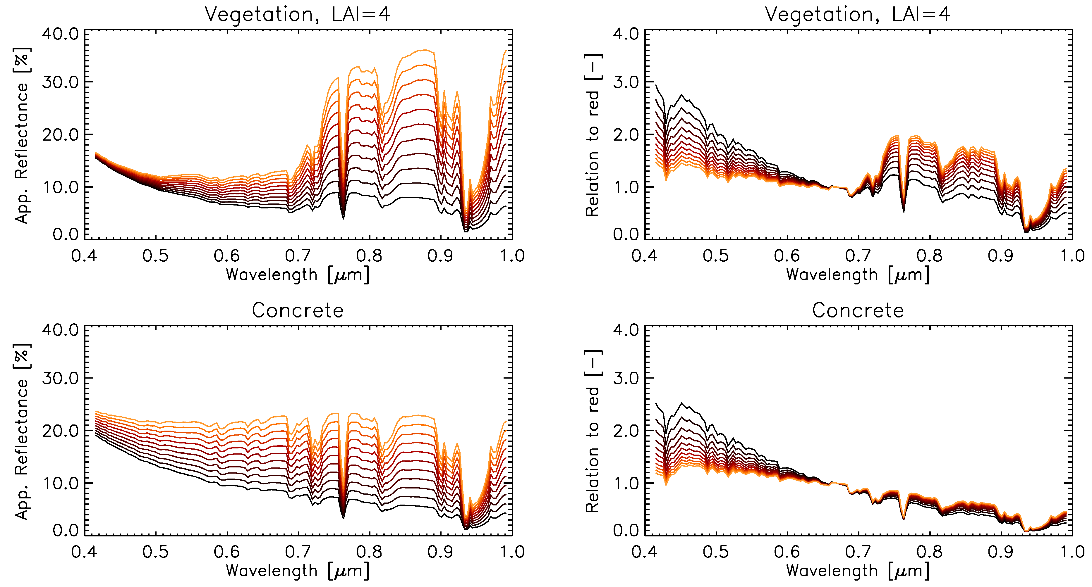
Figure 2.
Aerosol dependency of index mean values for flight altitudes h = 2 km, h = 5 km above ground and for the top of atmosphere level. left: red to blue ratio index (Equation (3)) for simulated apparent reflectances. The dotted curves show the dark object apparent reflectance in the blue for the three flight levels. right: the result of an optimized normalization using the dark object signatures (Equation (4)).

Figure 3.
Signatures of shadow on water (left) and normalization to trend line (right). Plot for satellite level and 20 km visibility.
Figure 3.
Signatures of shadow on water (left) and normalization to trend line (right). Plot for satellite level and 20 km visibility.

Figure 4.
Derivation of cast shadow mask from original image by calculating land index, water index, water mask, and a combination of both and applying a threshold of 0.33 to the output. The indices (in blue) are linearly scaled between 0.2 and 0.6 in this sample.
Figure 4.
Derivation of cast shadow mask from original image by calculating land index, water index, water mask, and a combination of both and applying a threshold of 0.33 to the output. The indices (in blue) are linearly scaled between 0.2 and 0.6 in this sample.

Figure 5.
Dependency of cast shadow correction results from chosen aerosol amount: ATCOR-4 surface reflectance retrieval results for visibility values between 8 and 30 km, applying cast shadow correction.
Figure 5.
Dependency of cast shadow correction results from chosen aerosol amount: ATCOR-4 surface reflectance retrieval results for visibility values between 8 and 30 km, applying cast shadow correction.
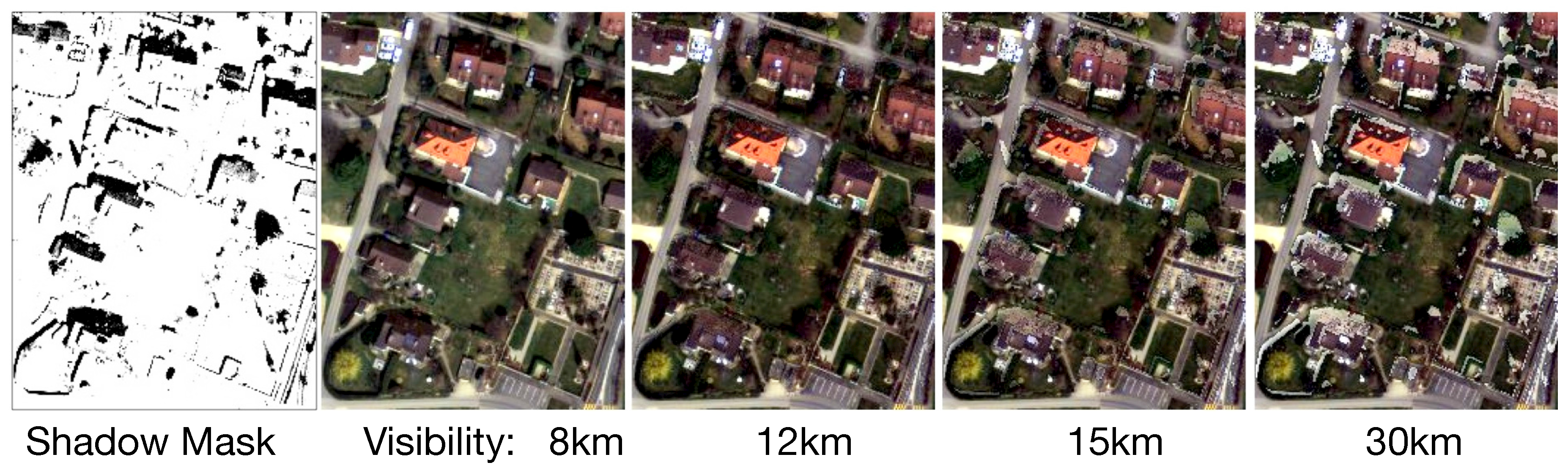
Figure 6.
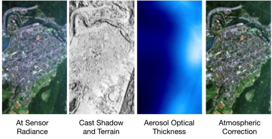
Flowchart of atmospheric correction using cast shadow detection and automated aerosol optical thickness (AOT) retrieval.
Figure 6.
Flowchart of atmospheric correction using cast shadow detection and automated aerosol optical thickness (AOT) retrieval.

Figure 7.
Top left: Airborne digital system (ADS) raw imagery; top right: cast shadow detection results, combined with illumination factor ; bottom left: shadow correction result; bottom right: aerosol retrieval masks; orange: cast shadows, yellow: bright reference areas (reproduced by permission of Federal Office of Topography swisstopo BA17083).


Figure 8.
Shadow detection results for ADS samples.

Figure 9.
Shadow detection results for APEX samples.
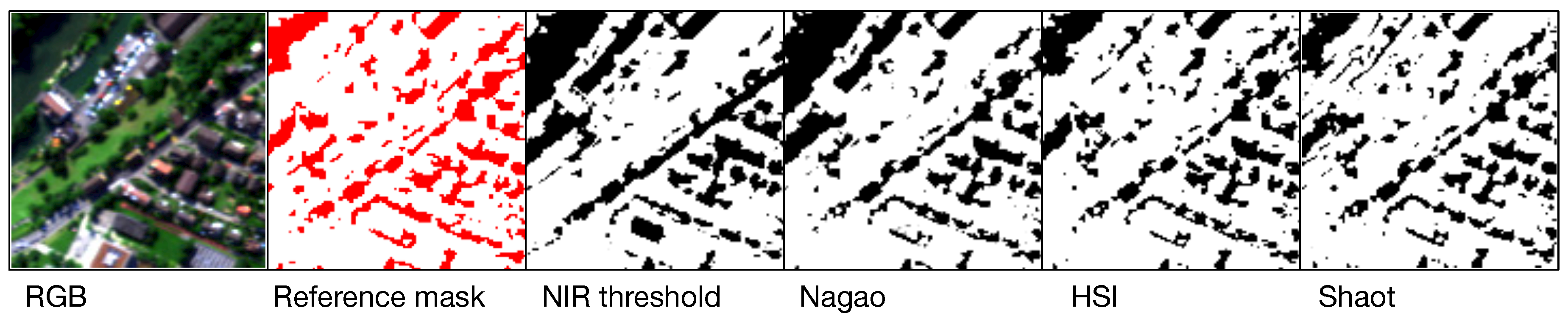
Figure 10.
APEX shadow detection result examples; left: true color red-green-blue (RGB) subset; middle: index combination as RGB, with Red: water index, Green: land index, Blue: average reflectance red-nir; right: fractional illumination shading as cast shadow detection result in combination with terrain based shading.
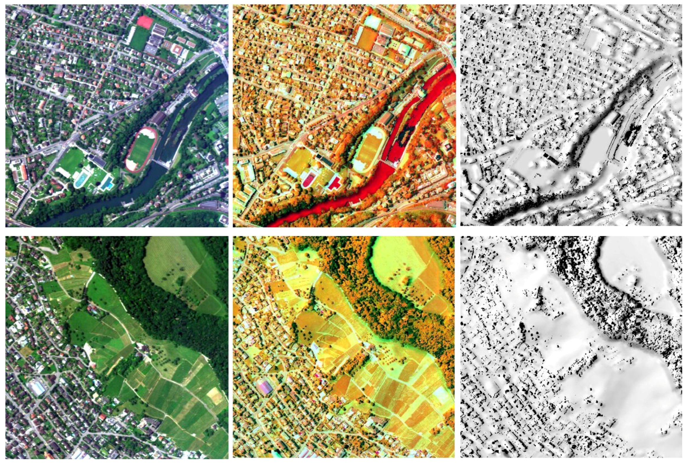
Figure 11.
APEX aerosol retrieval and correction for the Laegern scene of 29 June 2010. left: at-sensor radiance; 2nd: fractional illumination as combination of cast shadow and terrain based illumination from smoothed digital surface model; 3rd: aerosol optical thickness from shadow based aerosol retrieval (SHAOT); 4th: ATCOR-4 atmospheric and topographic correction result with SHAOT method; right: ATCOR-4 atmospheric and topographic correction result with dark dense vegetation (DDV) method.
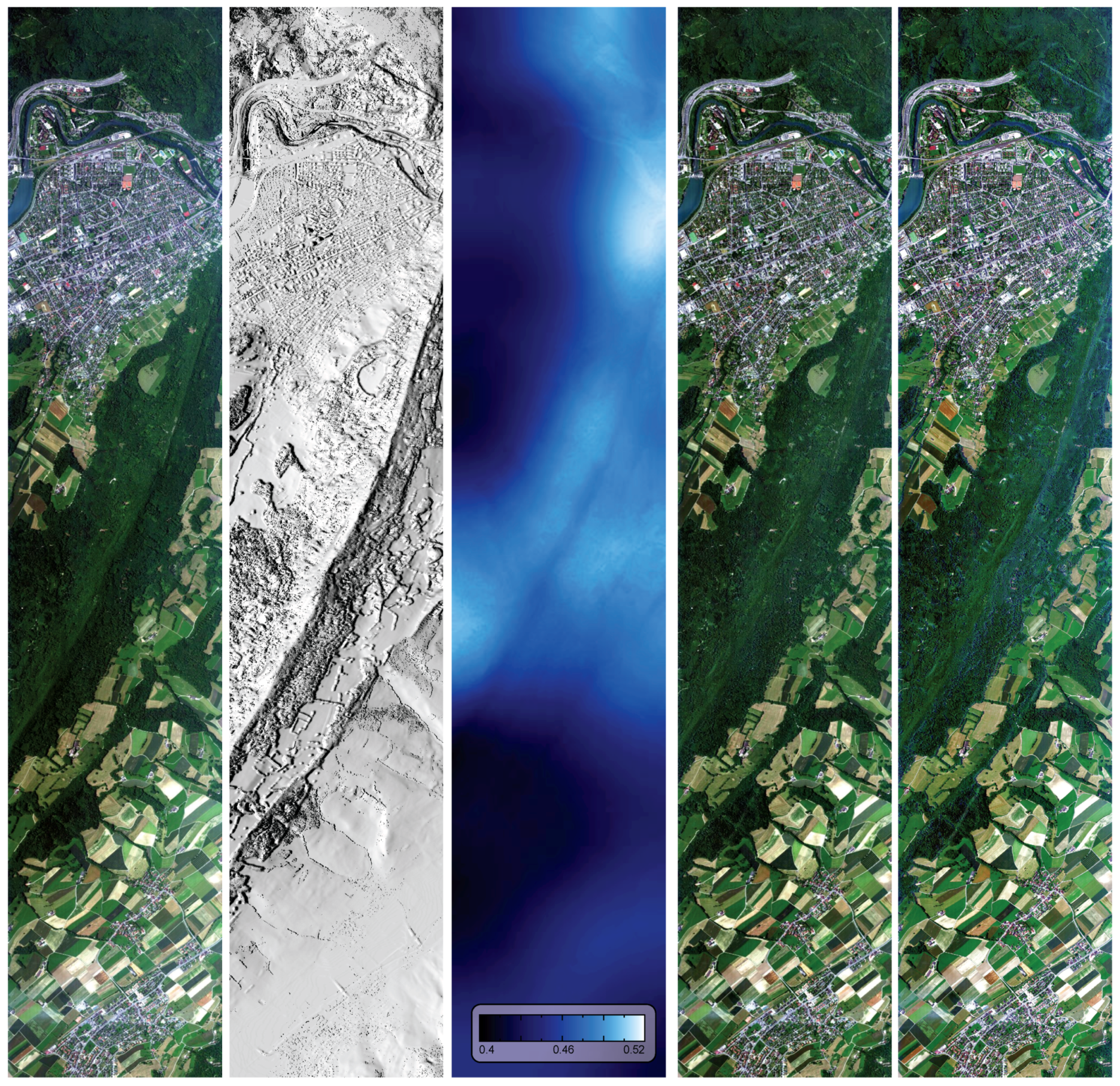
Figure 12.
Spectral impact of aerosol content estimation using the DDV and the SHAOT method on atmospheric compensation results for six reference objects and two acquisition dates.
Figure 12.
Spectral impact of aerosol content estimation using the DDV and the SHAOT method on atmospheric compensation results for six reference objects and two acquisition dates.

Figure 13.
ADS-100 atmospheric processing using variable aerosols based on SHAOT method. Mosaic of three consecutive images. Top: digital elevation model (DEM); 2nd: at-sensor radiance image and validation sample locations; 3rd: AOT distribution; 4th: atmospheric compensation result using SHAOT aerosols; 5th: atmospheric compensation using fixed standard aerosol amount. The position of the analyzed image patches are indicated in red and the spectral sample targets locations are indicated in green for ’asphalt’ and in yellow for ’lake’. The data has been scaled in east-west direction by 50% for better visualization (reproduced by permission of Federal Office of Topography swisstopo BA17083).

Figure 14.
Reflectance outputs from ADS atmospheric processing for asphalt and lake water in comparison to reference spectra (black lines). The dashed lines are the standard atmospheric compensation results whereas the solid colored lines are from SHAOT processing.
Figure 14.
Reflectance outputs from ADS atmospheric processing for asphalt and lake water in comparison to reference spectra (black lines). The dashed lines are the standard atmospheric compensation results whereas the solid colored lines are from SHAOT processing.


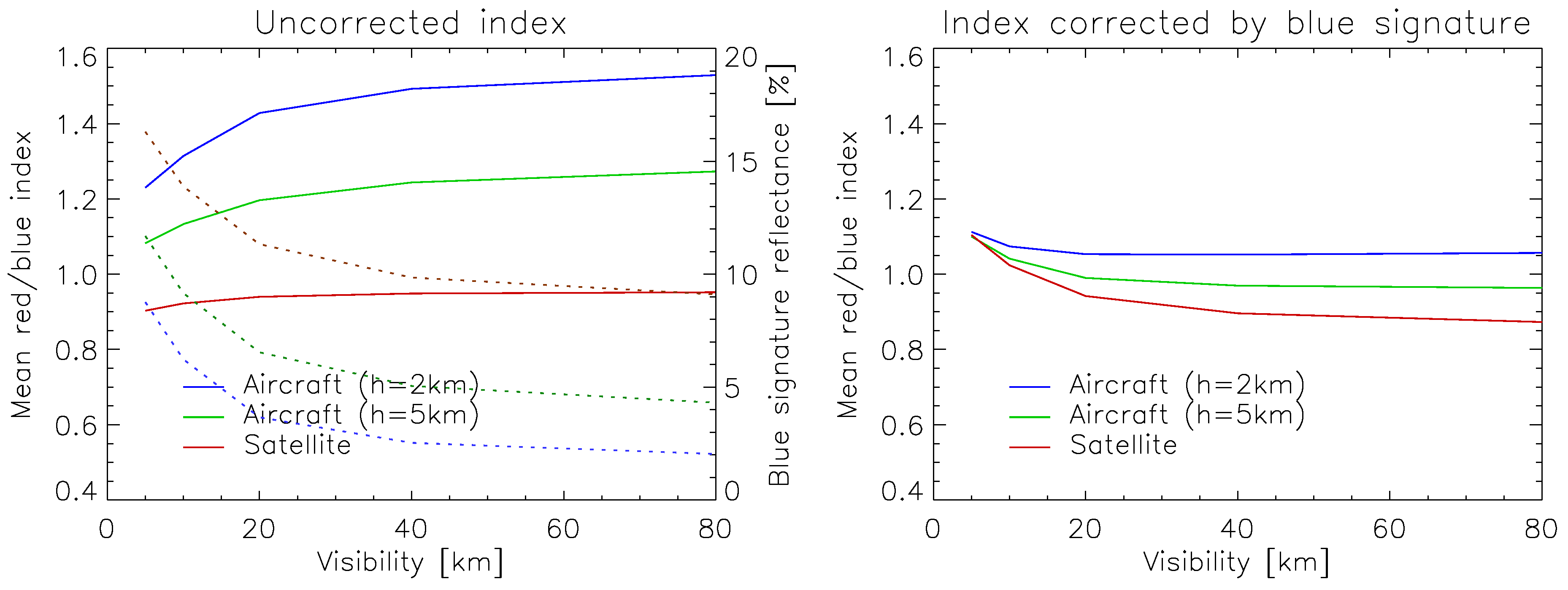
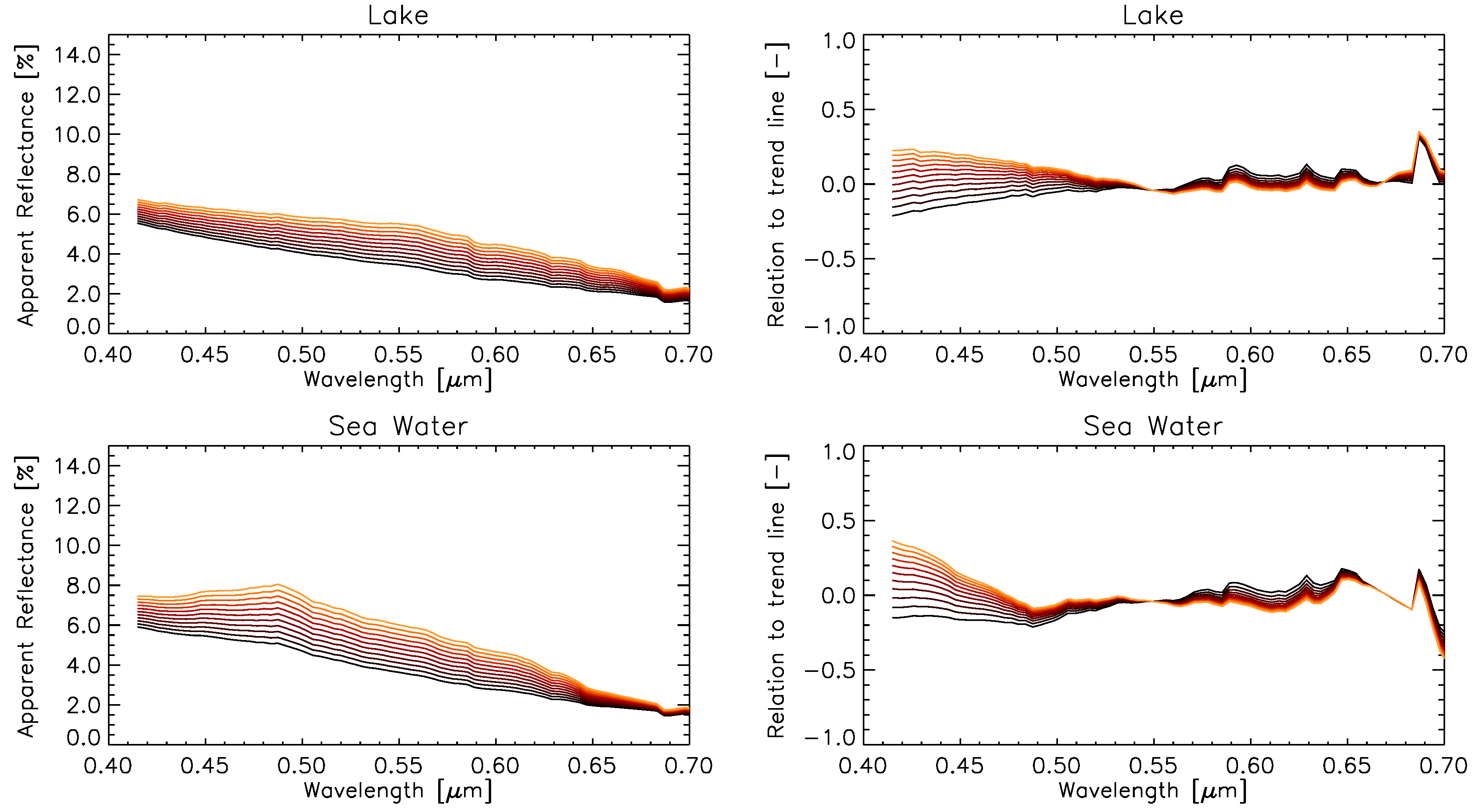
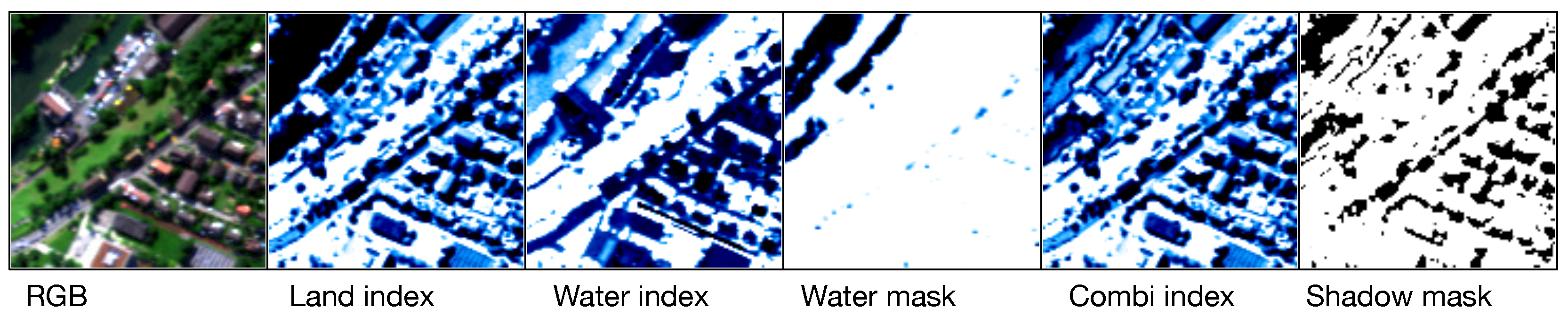
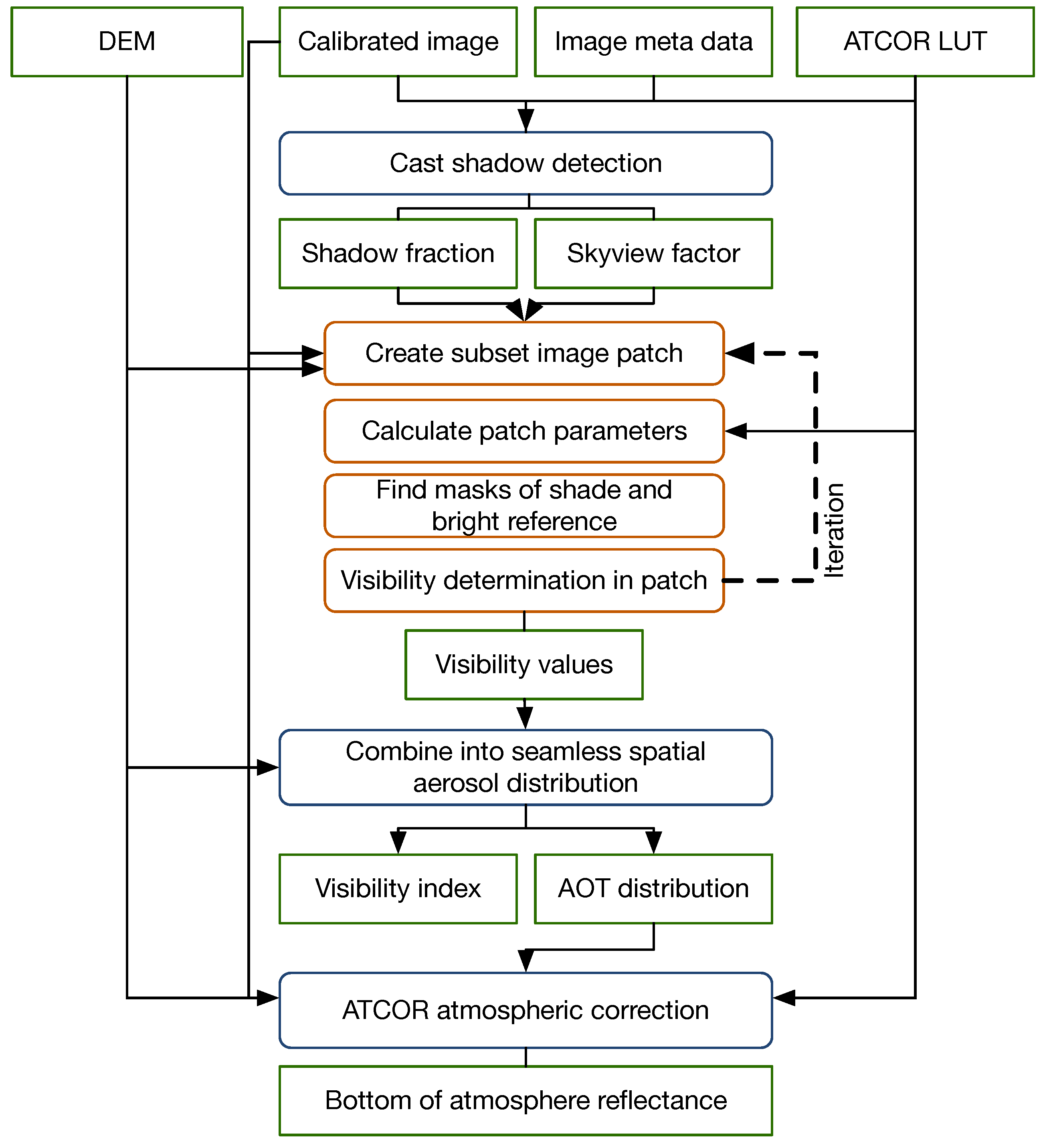
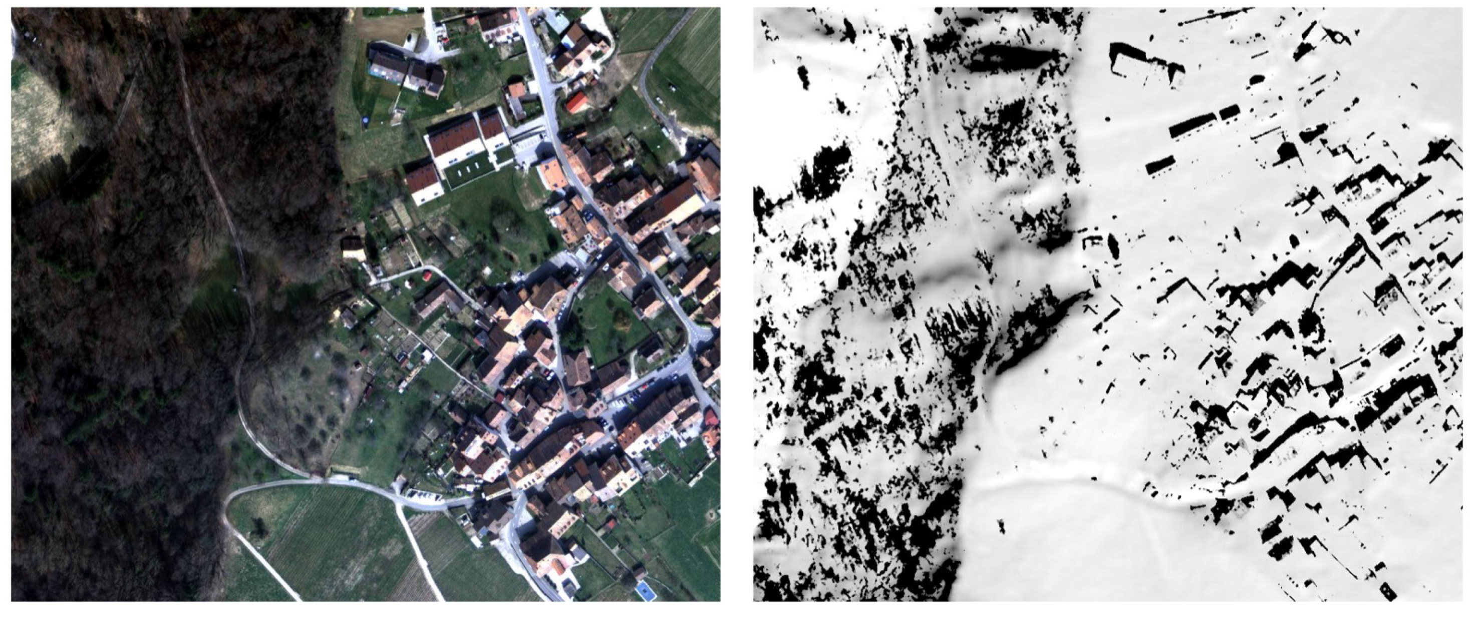
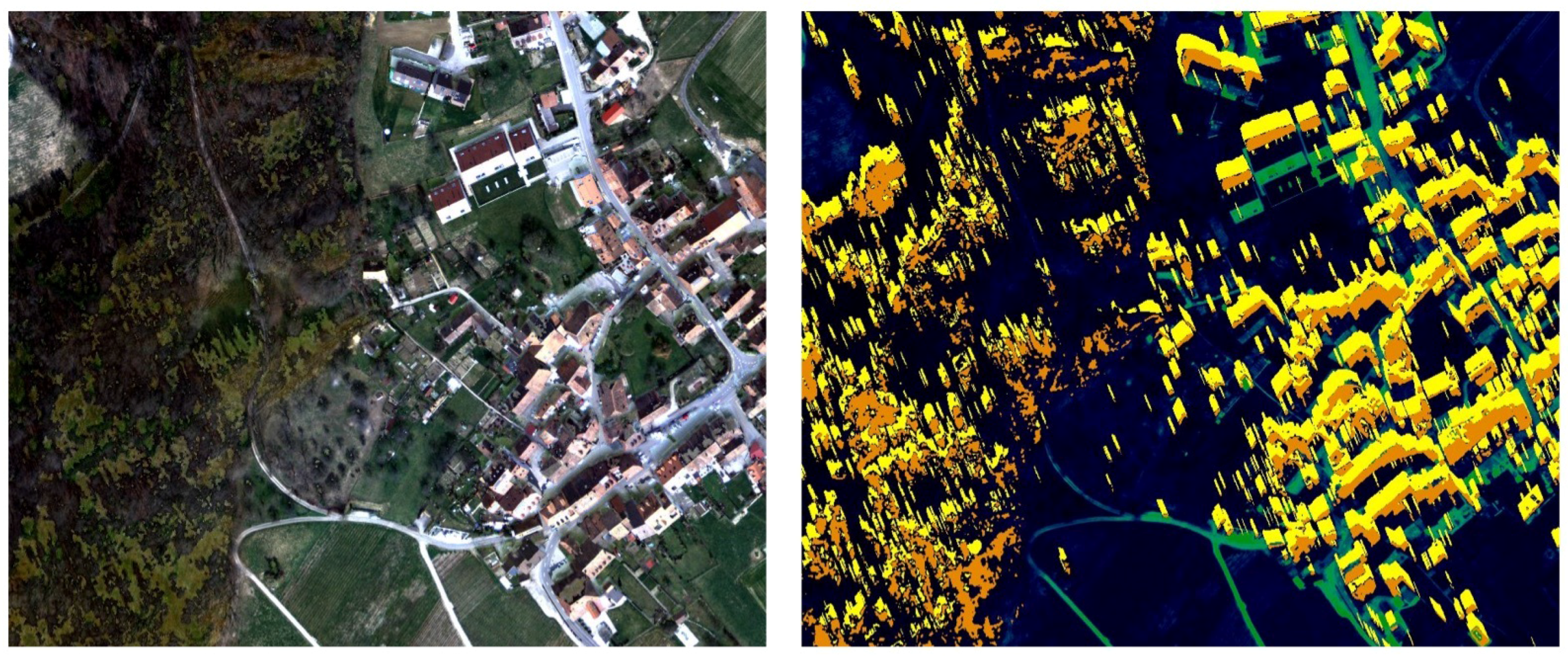
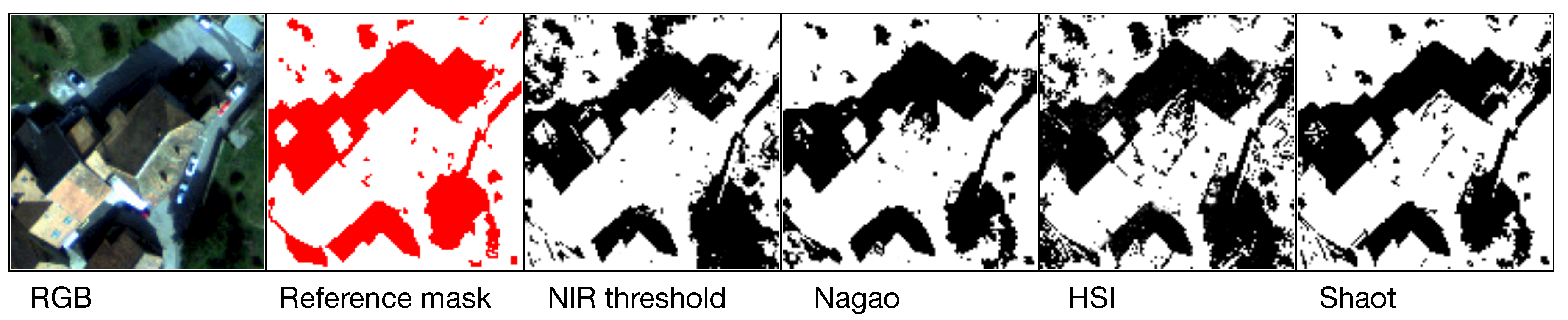
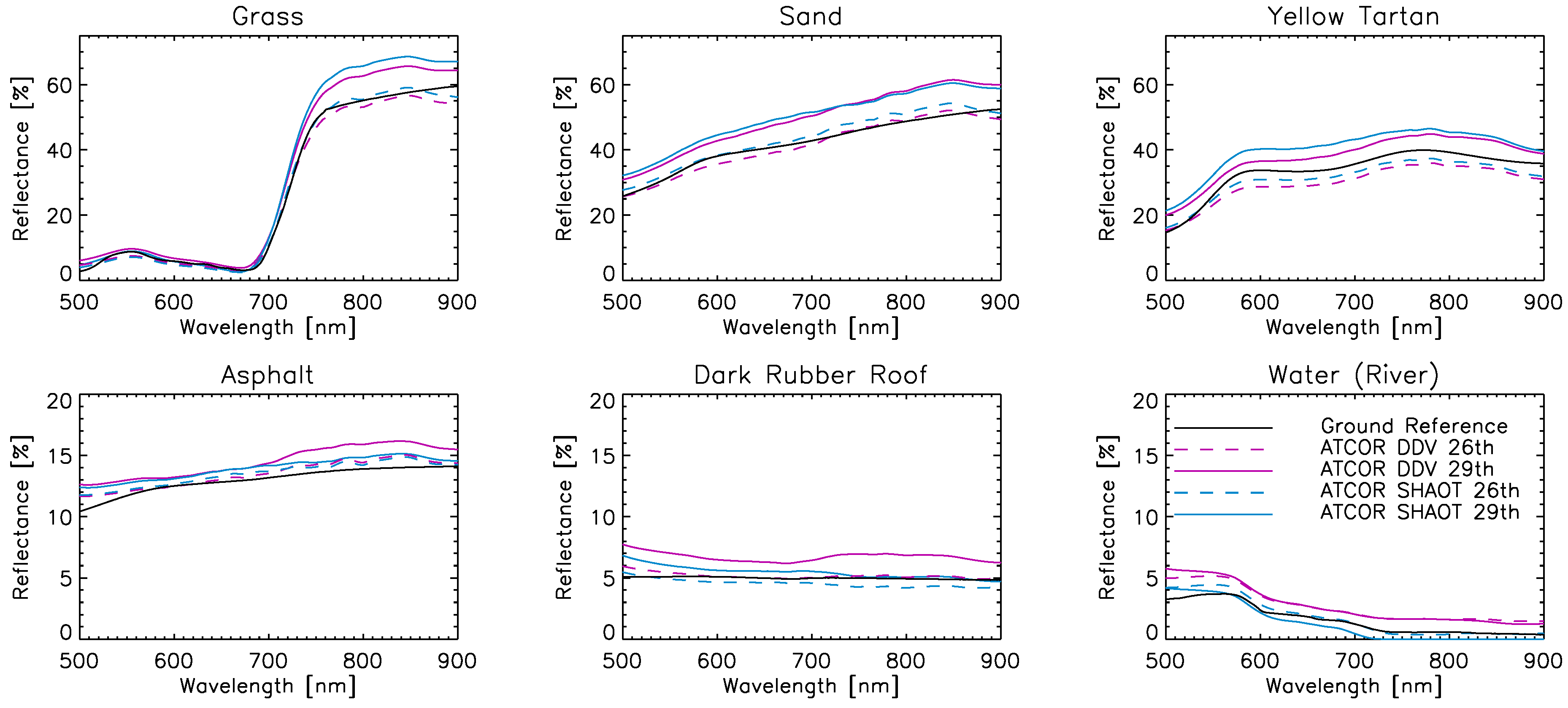
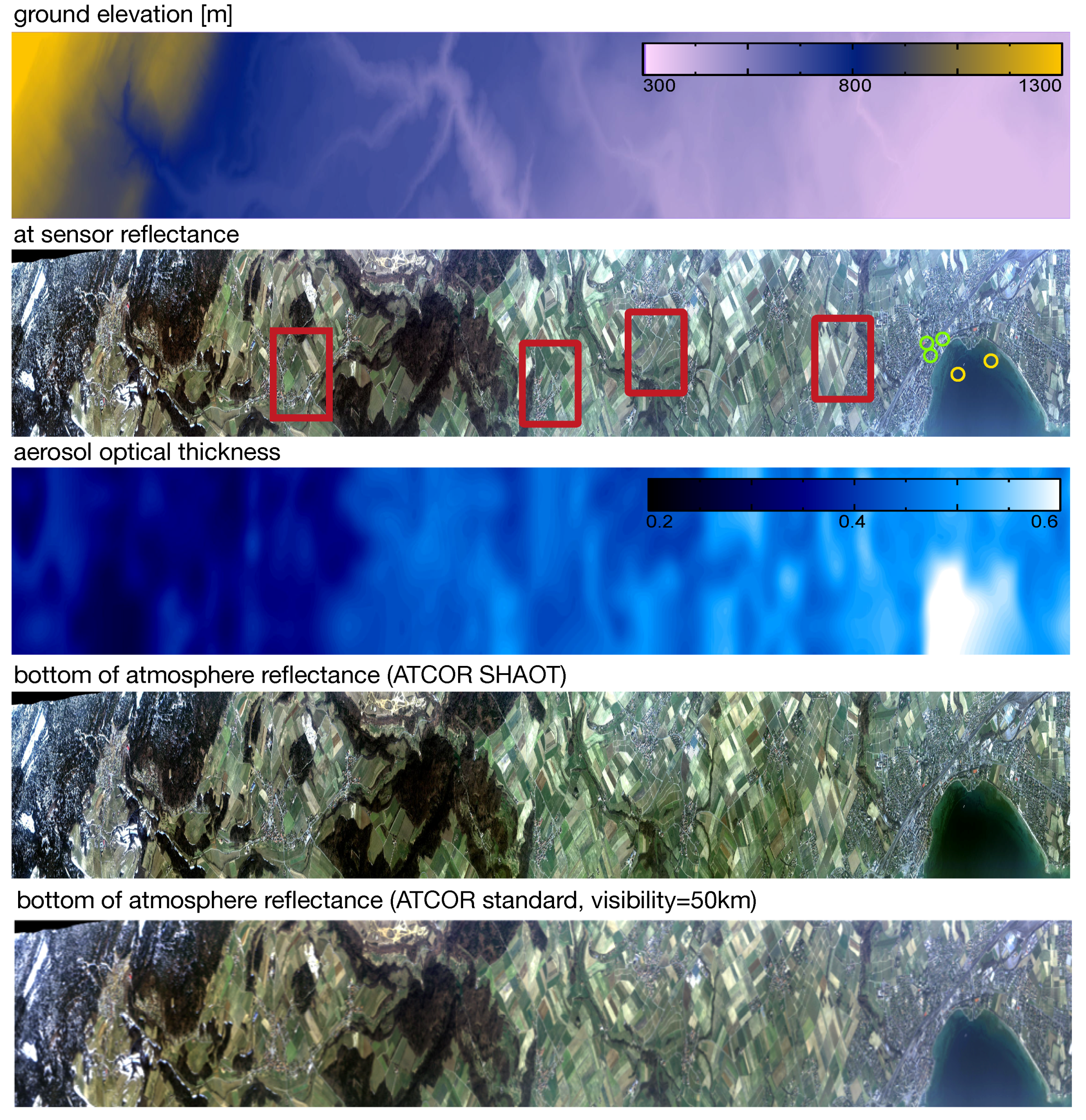
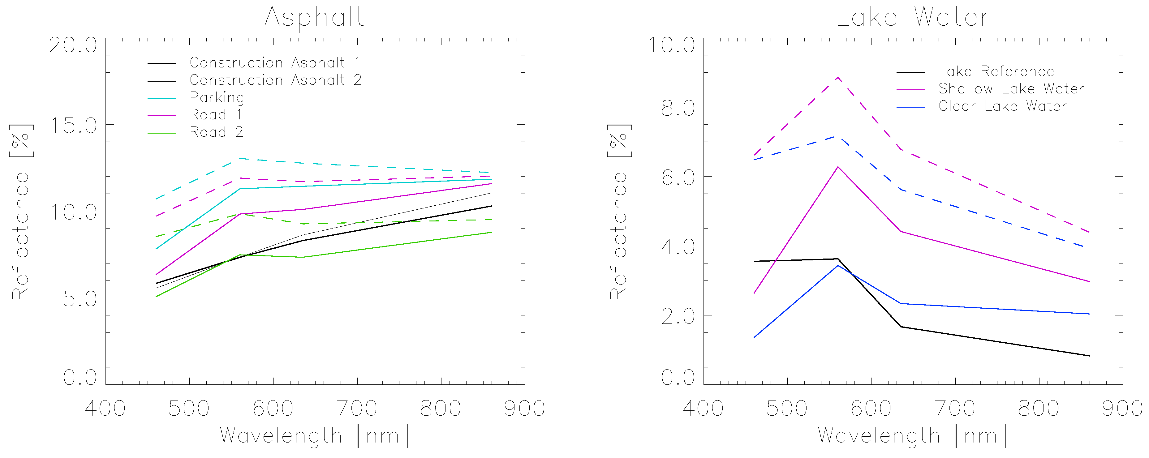
Table 1.
Sensitivity of aerosol retrieval on various error sources for 0.25 m resolution data, given as percentage error in aerosol optical thickness (AOT). The (+) sign is added whenever systematic increases are observed, whereas the other values are statistical variation levels.
Table 1.
Sensitivity of aerosol retrieval on various error sources for 0.25 m resolution data, given as percentage error in aerosol optical thickness (AOT). The (+) sign is added whenever systematic increases are observed, whereas the other values are statistical variation levels.
| Error Source | Forest | Settlement | Remarks |
|---|---|---|---|
| overestimate cast shadow | (+) 13.5% | (+) 51.7% | includes directly illuminated areas |
| underestimate cast shadow | 5.8% | 6.4% | no clear trend |
| vary reference shift distance | 0.4% | 1.8% | in steps of 1 m |
| vary reference angle | 6.0% | 0.9% | in steps of |
| neglect skyview factor | (+) 5.2% | (+) 5.3% | set to 100% |
| neglect adjacency effect | (+) 30.0% | (+) 52.4% | no adjacency correction |
Table 2.
Classification accuracy (kappa values) on two sample images for four various shadow detection methods.
Table 2.
Classification accuracy (kappa values) on two sample images for four various shadow detection methods.
| Test Case | NIR Threshold | Nagao Method | HSI Inversion | SHAOT Method |
|---|---|---|---|---|
| ADS (airborne digital system) | 69% | 82% | 71% | 85% |
| APEX (airborne prism experiment) | 46% | 62% | 75% | 76% |
NIR: near infrared; HSI: Hue-Saturation-Intensity
Table 3.
In-scene consistency analysis between two image patches on the blue and the NIR band of ADS imagery, comparing apparent at-sensor reflectance values ( and ) to the standard reflectance products ( and ) and the dark dense vegetation (DDV) and SHAOT based reflectance outputs.
Table 3.
In-scene consistency analysis between two image patches on the blue and the NIR band of ADS imagery, comparing apparent at-sensor reflectance values ( and ) to the standard reflectance products ( and ) and the dark dense vegetation (DDV) and SHAOT based reflectance outputs.
| Altitude [m] | |||||||||||
|---|---|---|---|---|---|---|---|---|---|---|---|
| Sample 1 | 705 | 0.51 | 0.36 | 7.8 | 23.4 | 6.7 | 24.7 | 5.3 | 25.7 | 5.0 | 25.2 |
| Sample 2 | 609 | 0.14 | 0.44 | 8.7 | 28.0 | 7.7 | 29.6 | 3.9 | 29.3 | 5.3 | 30.7 |
| Sample 3 | 524 | 0.14 | 0.44 | 8.8 | 26.6 | 7.7 | 28.2 | 3.8 | 27.9 | 5.2 | 29.2 |
| Sample 4 | 425 | 0.16 | 0.50 | 9.6 | 22.4 | 8.6 | 23.7 | 8.6 | 23.5 | 5.6 | 24.5 |
| Mean | 8.7 | 25.1 | 7.7 | 26.6 | 5.4 | 26.6 | 5.3 | 27.4 | |||
| Mean Deviation | 0.5 | 2.2 | 0.5 | 2.4 | 1.6 | 2.0 | 0.2 | 2.6 |
© 2018 by the authors. Licensee MDPI, Basel, Switzerland. This article is an open access article distributed under the terms and conditions of the Creative Commons Attribution (CC BY) license (http://creativecommons.org/licenses/by/4.0/).
Share and Cite
MDPI and ACS Style
Schläpfer, D.; Hueni, A.; Richter, R. Cast Shadow Detection to Quantify the Aerosol Optical Thickness for Atmospheric Correction of High Spatial Resolution Optical Imagery. Remote Sens. 2018, 10, 200. https://doi.org/10.3390/rs10020200
AMA Style
Schläpfer D, Hueni A, Richter R. Cast Shadow Detection to Quantify the Aerosol Optical Thickness for Atmospheric Correction of High Spatial Resolution Optical Imagery. Remote Sensing. 2018; 10(2):200. https://doi.org/10.3390/rs10020200
Chicago/Turabian StyleSchläpfer, Daniel, Andreas Hueni, and Rudolf Richter. 2018. "Cast Shadow Detection to Quantify the Aerosol Optical Thickness for Atmospheric Correction of High Spatial Resolution Optical Imagery" Remote Sensing 10, no. 2: 200. https://doi.org/10.3390/rs10020200
Note that from the first issue of 2016, this journal uses article numbers instead of page numbers. See further details here.