Reconstructing Seabed Topography from Side-Scan Sonar Images with Self-Constraint


1
School of Geodesy and Geomatics, Wuhan University, 129 Luoyu Road, Wuhan 430079, China
2
Institute of Marine Science and Technology, Wuhan University, 129 Luoyu Road, Wuhan 430079, China
3
Automation Department, School of Power and Mechanical Engineering, Wuhan University, 8 South Donghu Road, Wuhan 430072, China
*
Author to whom correspondence should be addressed.
Remote Sens. 2018, 10(2), 201; https://doi.org/10.3390/rs10020201
Submission received: 22 November 2017
/
Revised: 22 January 2018
/
Accepted: 26 January 2018
/
Published: 29 January 2018
(This article belongs to the Special Issue Instruments and Methods for Ocean Observation and Monitoring)
Abstract
:To obtain the high-resolution seabed topography and overcome the limitations of existing topography reconstruction methods in requiring external bathymetric data and ignoring the effects of sediment variations and Side-Scan Sonar (SSS) image quality, this study proposes a method of reconstructing seabed topography from SSS images with a self-constraint condition. A reconstruction model is deduced by Lambert’s law and the seabed scattering model. A bottom tracking method is put forward to get the along-track SSS towfish heights and the initial seabed topography in the SSS measuring area is established by combining the along-track towfish heights, towfish depths and tidal levels obtained from Global Navigation Satellite System (GNSS). The complete process of reconstructing seabed topography is given by taking the initial topography as self-constraint and the high-resolution seabed topography is finally obtained. Experiments verified the proposed method by the data measured in Zhujiang River, China. The standard deviation of less than 15 cm is achieved and the resolution of the reconstructed topography is about 60 times higher than that of the Digital Elevation Model (DEM) established by bathymetric data. The effects of noise, suspended bodies, refraction of wave in water column, sediment variation, the determination of iteration termination condition as well as the performance of the proposed method under these effects are discussed. Finally, the conclusions are drawn out according to the experiments and discussions. The proposed method provides a simple and efficient way to obtain high-resolution seabed topography from SSS images and is a supplement but not substitution for the existing bathymetric methods.

1. Introduction
High-resolution seabed topography has important applications in offshore oil exploration [1], underwater target detection [2], marine eco-environmental protection [3,4], underwater navigation and localization [5] and many other fields. Acoustic waves move quite efficiently through water and the ability to travel over such great distances allows remote sensing in a water environment, which is helpful for ocean observation and monitoring. Devices that use acoustic waves in such applications fall under the family of instruments known as sonars. Currently, the most widely used sonars in the bathymetric field are single-beam bathymetric system (SBS) and multibeam bathymetric system (MBS). Using SBS to obtain high-resolution seabed terrain needs dense surveying lines, which are low-efficiency and high-cost. Using MBS, one can carry out a large-scale bathymetric measurement, but the interval of surveying points in a ping will be enlarged and the bathymetric resolution will be decreased with the increases of water depth and beam incident angle [6,7,8]. Side-scan sonar (SSS) is widely used to reflect seabed surface features. The SSS transducer built in a towfish is usually towed behind a surveying vessel by a cable, it emits a wide-angle beam and receives the seabed echoes at fixed time intervals to form the seabed image. The resolution of a SSS image is about 20–100 times larger relative to that of MBS bathymetric topography. Consequently, SSS images can vividly reflect the seabed targets, topography and sediment reflectivity [9,10]. If the micro-topography features can be determined from SSS images, it will be helpful to obtain the high-resolution seabed topography in deep sea. In addition, in the shallow waters, although the MBS can achieve resolution of decimeter scale, the reconstruction method from SSS images can also provide an efficient and low-cost supplement to obtain high-resolution seabed topography.
Shape from shading (SFS) is an efficient technique to obtain the three-dimensional (3D) shape from the intensity variation of the two-dimensional (2D) image. In SFS, the reconstruction of the 3D shape is based on the illumination theory and the imaging mechanism [11,12,13]. As early as 1999, Bell et al. studied the SSS imaging mechanism, analyzed the effects of acoustic wave incident directions on the seabed texture presentations in SSS images, and qualitatively discussed the relationship between the incident directions and the seabed texture images [14]. The research implies that the seabed topography reconstruction is related to the incident direction. On this basis, many scholars have developed studies on reconstructing 3D seabed topographies using 2D SSS images. Johnson et al. studied the 3D shape reconstruction of seabed topography by different seabed scattering models, and concluded that Lambert’s law is appropriate [15,16].
To get absolute seabed topography from the SSS image, many scholars developed different seabed reconstruction methods [17,18,19,20,21,22]. These studies can be classified into two categories according to whether the reconstruction needs the external bathymetric data. Under the support of external bathymetric data, Lange et al. obtained the seabed topography of every ping by a propagation method [17]. The method obtained the position and seabed height of the first echo of each ping using the external bathymetric data firstly, and then built seabed elevation maps from SSS waterfall images according to the propagation principle of acoustic wave in water. Johnson et al. used external bathymetric data to build an initial terrain for the reconstruction process from SSS images [15,16]. Bikonis K et al. combined MBS and SSS data to build the statistical curves, namely the seabed backscattering coefficient angular dependence curves to reconstruct the seabed relief in a flat experimental area. As stated by Bikonis et al., the method needed to be further verified and improved for wide applications [18]. Zhao and Wang et al. studied the relationship between the reconstructed seabed topography and the bathymetric data, and discovered the strong correlation between them. A large-scale seabed topography inversion was carried out by Lambert’s law, and the absolute seabed topography was obtained through adjusting the inversion result by the correlation model [19,20]. The above studies need the bathymetric data as an external constraint, and thus the reconstruction results may be easily affected by the data quality [19]. Moreover, an extra SBS or MBS measurement has to be performed. Without the external bathymetric data, Dura et al. analyzed the propagation method and pointed out that the method simplifies the reconstruction of seabed topography, but it is more sensitive to noise and abnormal ping measurement, and thus they proposed a linear method to reconstruct the textured seabed from synthetic SSS images [21]. Using the linear method, Dura et al. reconstructed the relative shapes of sand ripples [21]. The quantitative evaluation of the reconstruction showed that the linear method had better robustness than the propagation method [21]. The conclusion was achieved by simulation experiments and it needs to be further verified by the actual data. Besides, Coral et al. used an assumed flat initial seabed to reconstruct the absolute seabed topography from the SSS image by combining the expectation-maximization and multiresolution algorithms, but they obtained the reconstructed small-size shapes with large quantization errors [22].
To simplify the reconstruction and get accurate seabed topography without the constraint of external bathymetric data, this paper proposes a novel method to reconstruct seabed topography from SSS images with the SSS self-constraint which can be obtained by combining the SSS towfish height from the SSS waterfall image, the SSS towfish depth provided by a built-in pressure sensor and GNSS tidal level observed by the GNSS receiver mounted in surveying vessel. The paper is organized as follows. Section 2 deduces the reconstruction model using SSS images. Section 3 solves the model using Newton iteration algorithm, gives a method to extract the along-track depth from SSS waterfall images, and proposes the process of reconstructing 3D seabed topography using SSS images by taking the extracted along-track depth as self-constraint. Section 4 designs experiments to verify the proposed method and theoretically analyzes the results and assesses the accuracies of reconstructed seabed topographies. Section 5 discusses the influencing factors on the proposed method. Section 6 draws the conclusions according to the experiments and the discussions.
2. Reconstruction Model of 3D Seabed Topography
The acoustic waves emitted from the SSS transducer propagate through sea water to seabed, and the echoes from the seabed are received by the transducer at fixed time intervals. SSS images are formed by converting the backscatter strength (BS) to the gray level. The BS or gray level is related to the incident acoustic energies and directions, the seabed albedo and the topography gradients [9]. It is generally believed that the seabed is mainly comprised of diffuse scattering characteristics, and Lambert’s law is an appropriate model to describe the scattering process [23,24,25,26,27]. In optics, Lambert’s law says that the radiant intensity or luminous intensity observed from an ideal diffusely reflecting surface or ideal diffuse radiator is directly proportional to the cosine of the angle θ between the direction of the incident light and the normal vector [28]. This law is also suitable for acoustics measurement. A lot of coarse surfaces which obey Lambert’s law are called Lambertian and exhibit Lambertian reflectance. When given the parameter of incident direction, the Lambert’s law can be used to redistribute the acoustic energy [23]. Figure 1 describes the relationship between the BS and the seabed topography gradients [23].
Es is proportional to the cosine of the incident angle θ, and can be expressed as
where, u is the albedo, other parameters have the same meanings as shown in Figure 1. Let A = EicosδdS, Equation (1) can be simplified as
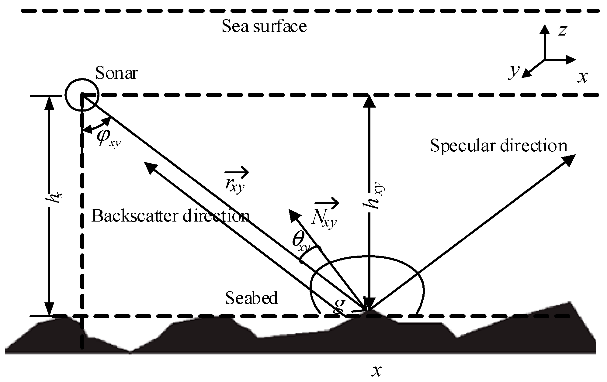
Equation (2) quantitatively describes the relationship between BS and the topography gradient. Figure 2 shows the situation of starboard transducer receiving echo under towfish reference frame (TFS). TFS is a right-hand coordinate system. The origin point, x, y and z axles of TFS are defined as the center of SSS transducer, the ping scanning line direction, the tracking direction and the direction perpendicular to the xoy surface.
Figure 2 simplifies the SSS transducer as a point source, and treats the propagation path as a straight line. After time varying gain (TVG) correction and radiation correction, the acoustic waves hitting on the seabed surface have the same incident energy [29,30,31]. For the homogeneous seabed, u is often set as a constant. Define Inorm = Es/Au
where, Inorm is called the normalized intensity, (x, y) are the coordinates of point g, θ reflects the topography gradient variations. The relationship of incident angle θ, incident vector and the normal vector can be expressed as
where, τxy is the tilt angle between the plane component of incident direction and x-axis, pxy and qxy are topography gradients along x and y directions, z is topography height, zx−1,y and zx,y−1 are the neighbor heights of current pixel (x, y). In TFS, τxy is zero. ϕxy can be computed by towfish height and initial seabed terrain.
where, x is the horizontal distance, hxy is the vertical distance from the point g to the xoy surface, hx is towfish height, zinxy is the initial depth value of point g, zinx is the initial depth value of the point beneath the SSS transducer. Other parameters have the same meanings as in Figure 2.
Combining Equations (3)–(7) to compute z, the reconstructed topography can be obtained.
3. Reconstructing Seabed Topography from SSS Image
3.1. Solution of Reconstruction Model
To take Equations (4)–(7) into Equation (3), Equation (8) is established
Transform the Equation (8) into Equation (9) as
By Taylor series expansion, Equation (9) is depicted as
where, fn−1 is the (n − 1)th iteration result or the nth initial value, Г(1), Г(2), …, Г(n) are the 1st − nth order terms, zn and zn−1 are the seabed heights achieved by nth and (n − 1)th iterations, zx,y, zx−1,y and zx,y−1 are the seabed heights of pixel (x, y), (x − 1, y) and (x, y − 1). If assuming that seabed topography changes slowly, the linear part, Г(1) in Equation (10) plays the most important role in solving the reconstruction model [32]. By Taylor series expansion of up to first order terms, the linear approximation of the Equation (10) is obtained as
where, , ax−1,y and ax,-y−1 have the similar formation as ax,y.
The Equation (11) can also be transformed as
To solve the Equation (12) by Newton iteration algorithm [33], Equation (13) is given as
By iteration operation, the final topographic height znxy is obtained and the seabed topography is reconstructed. In the reconstruction, the initial topography and the iteration terminal condition are required. Given the initial seabed topography z0x,y, the final seabed topography can be reconstructed after iteration operation. The iteration can be stopped by a given threshold, ε. ε can be determined from the convergence curve of the iteration, which is shown in Section 5.5.
3.2. Bottom Tracking and Initial Seabed Topography
Equation (13) shows that the seabed topography can be reconstructed from SSS images if the initial topography z0 is given. z0 is often provided by external bathymetric data, which means an extra measurement must be done. To simplify the work, the following proposes a method to obtain z0 by bottom tracking and combining towfish height, depth and tidal level.
In the SSS measurement, the first received echo is from the SSS transducer nadir. During the process of transmitting the beam and receiving the first echo, the transducer records nothing, and thus a blank area is formed in the SSS waterfall image. The width of the blank area represents the SSS towfish height [34,35]. If the first echo can be detected, the towfish height can also be obtained. Because of receiving nothing, BSs of the blank area are far lower than those of the seabed area. Therefore, the boundary point of two areas in a ping scanning line, namely the seabottom point, can be detected by calculating the BS differences of adjacent pixels and finding the maximum difference.
or
where, i0 is the pixel number or position of detected seabottom point in a ping sequences. G (BS) denotes gray level (backscatter strength), ΔGi (ΔBSi) is the gray level (BS) difference of i + 1 and i pixels. Then, the towfish height htowfish can be calculated by
where, W and S are the width and the maximum slant range of the waterfall image.
To combine the towfish depth from the built-in pressure sensor and the tidal level measured by GNSS [36,37], the seabed height can be obtained by
where, z is the seabed height, Dtowfish is the towfish depth and T is the tidal level.
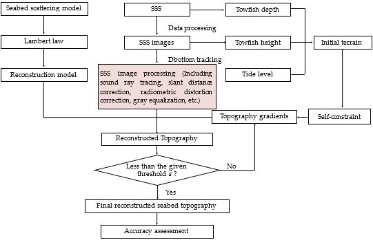
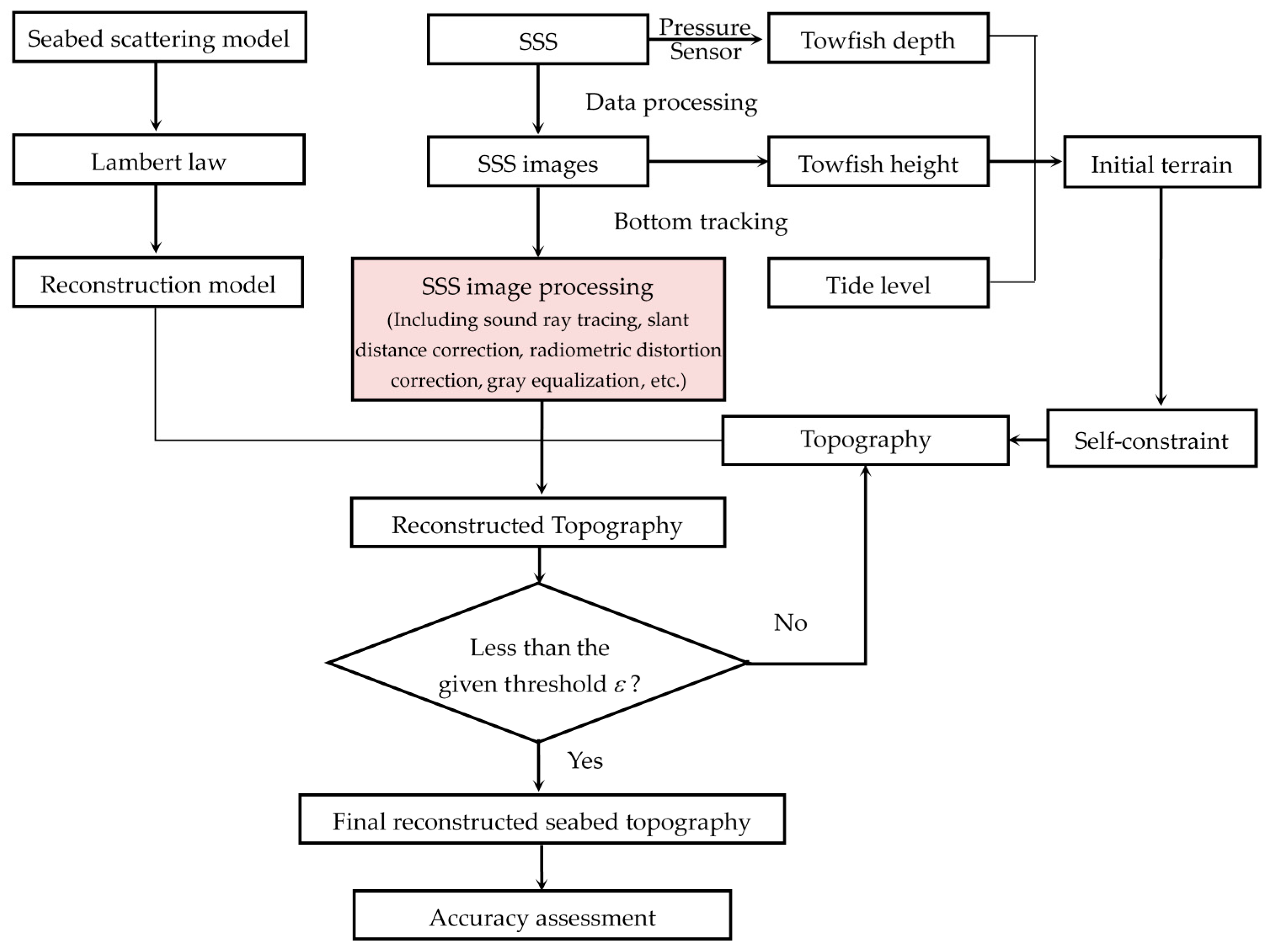
For the SSS image of a surveying line, the along-track seabed topographic sequence can be obtained by combining the towfish height derived from the waterfall image by the bottom tracking, towfish depth from the built-in pressure sensor and the tidal level measured by GNSS mounted on surveying ship. To reconstruct the seabed topography of the surveying line, the initial topography can be created by the method of triangulation with linear interpolation for the along-track seabed topographic sequences of the surveying line and those of its two adjacent surveying lines. Because the along-track topographic data is sparse in the coverage of the three SSS surveying lines, the created initial topography is coarse and used as the initial terrain in Equation (13) for reconstructing the seabed topography of the surveying line from the SSS image. Adopting a similar process to the above, the initial topographies can also be obtained for seabed reconstructions of other surveying lines. The process is depicted in Figure 3, which shows the initial topography is obtained from SSS waterfall images instead of the extra bathymetric data. Therefore, the initial topography or the constraint condition in the reconstruction is called self-constraint, which simplifies the reconstruction while saving costs.
3.3. Assessment
To assess if the system works, the evaluation of the reconstruction result needs to be implemented through computing the biases between the reconstructed data and the real bathymetric one. Using Equation (18), the maximum, minimum, mean and standard deviation of the biases can be computed and the probability distribution function (PDF) curves can be drawn. The obtained parameters and curves are used to assess the reconstruction method.
where, ΔD is the bias between the reconstructed data and the real bathymetric one, STD is the standard deviation, n is the number of points used in the assessment process.
3.4. Process of Reconstructing 3D Seabed Topography
The reconstruction process can be described in detail below (Figure 4):
- (1)
- Detect the seabottom points from SSS waterfall images to get the towfish heights, and then obtain the initial seabed topography by that depicted in Figure 3.
- (2)
- (3)
- Compute the topography gradients by Equation (6), the angle ϕ by Equation (7), and the seabed topography by Equation (13) using the self-constraint.
- (4)
- Execute iteration until the difference of two adjacent iterations is less than the given threshold ε. In the iteration, the next calculation uses the last result as the initial condition, and step (2) and step (3) are repeated until the difference meets Equation (14).
- (5)
- Assess the reconstruction by referring to the actual bathymetry data.
4. Experiments and Analysis
4.1. Experimental Area and Data Preparation
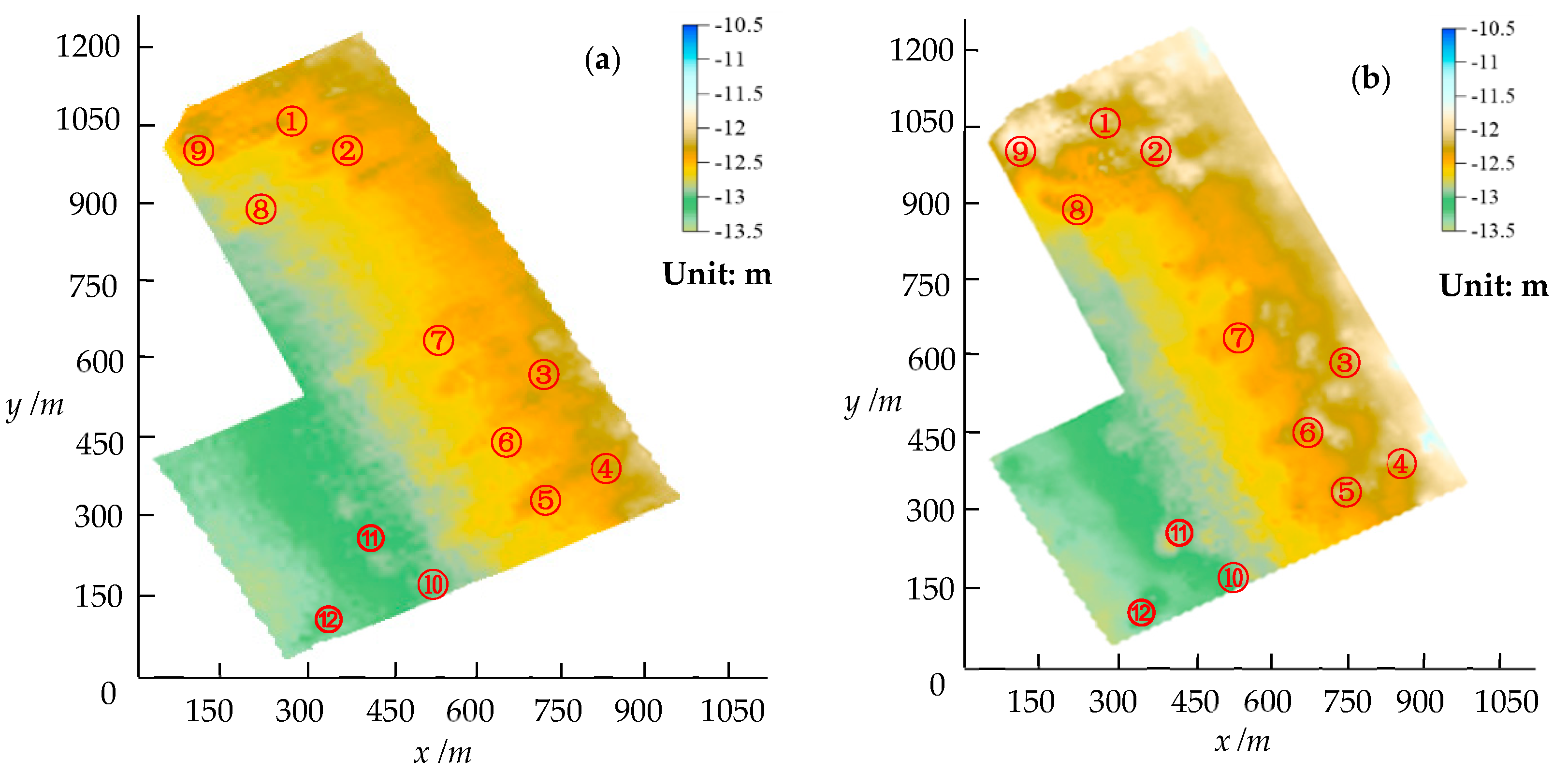
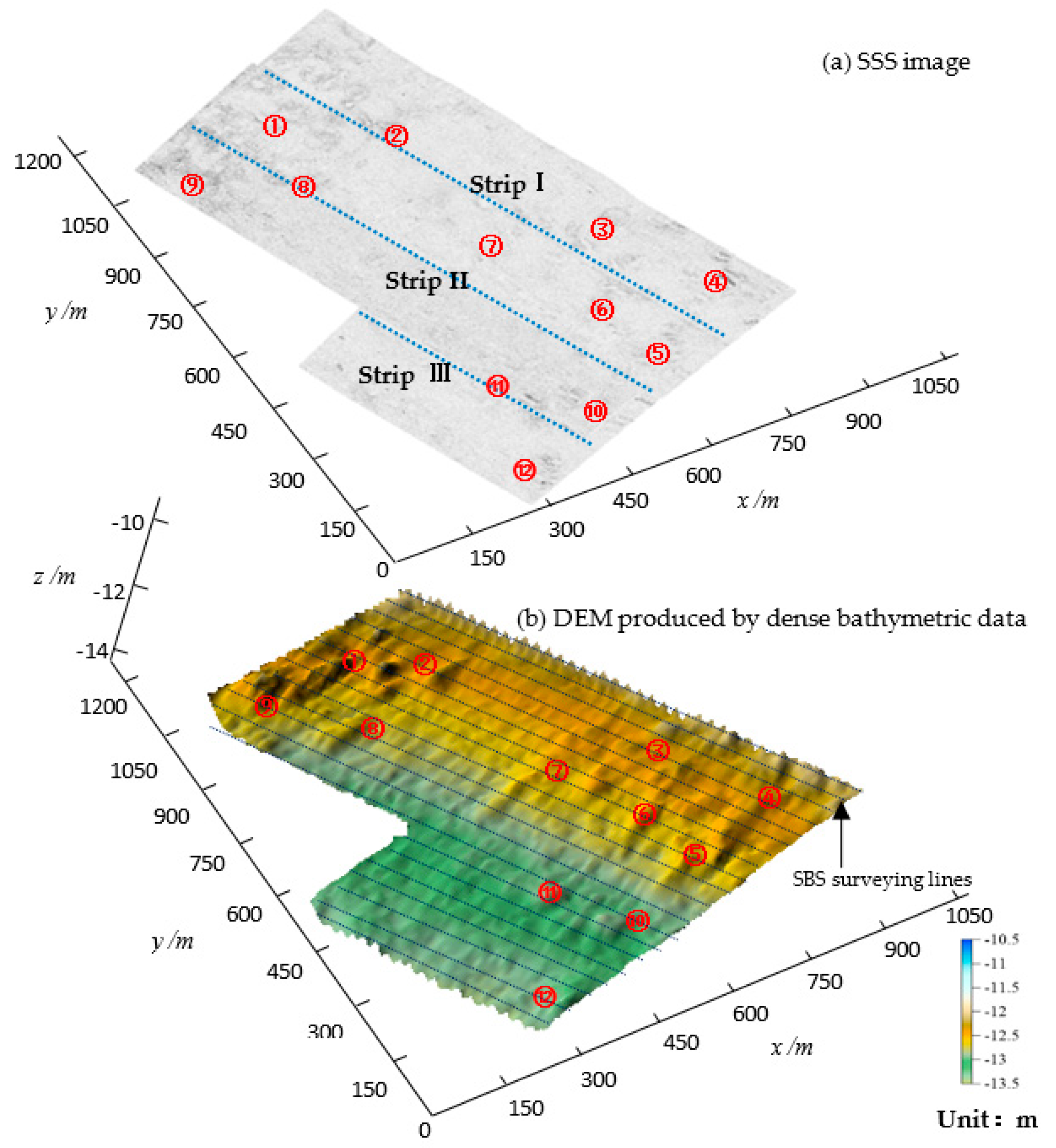
To verify the proposed method, an experiment was carried out in Zhujiang River with 10–14 m water depth, obvious seabed features and homogeneous sediment. In the experiment, Edgetech 4125 with 400 kHz sampling frequency, 2 cm lateral resolution, 0.6 m longitudinal resolution and 0.3° horizontal beam width, was adopted for the SSS measurement. The built-in pressure sensor with the accuracy of 0.5% depth was used to record the SSS towfish depth. Three surveying lines with the lengths of 1020 m, 900 m and 540 m were designed. The adjacent line interval and the SSS swath width are 200 m, and the overlapping ratio between adjacent lines is 50%. To assess the topography reconstructed by the proposed method, 20 surveying lines with 40 m interval were also accomplished by HY1600 with 208 kHz operating frequency, 8° beam angle, ±(0.01 m + 0.1% depth) bathymetric accuracy and 0.5 m along-track sampling interval in the area. In the measurement, the tidal level was also synchronously recorded. Raw SSS data were recorded in *.xtf files. To decode these files and deal with those by radiometric correction, slant range correction, geocoding and image mosaics, the image with the resolution of 0.6 m is formed as shown in Figure 5a. The features in the image are marked as ①–⑫. The bathymetric data are also processed by quality control, draft correction and tidal correction, and the Digital Elevation Model (DEM) is built as shown in Figure 5b. Features ①–⑫ are displayed clearly in Figure 5b. The results indicate the SSS image can reflect seabed features, and they also imply that the 3D shapes of these features can be recovered from a 2D SSS image. The corresponding 2D colored images are shown in Appendix A, which can also be used to compare.
4.2. Reconstructing Seabed Topography
To depict the reconstruction process in detail, Strip I is chosen. Before reconstructing the seabed topography, Strip I needs to be preprocessed. Firstly, the raw XTF file is decoded to form the waterfall image as shown in Figure 6a. Being affected by the propagation loss and absorption loss, the BSs will decrease with the increase of propagation range. TVG can compensate these losses to some extent. Being affected by beam pattern and TVG residual (or imperfect TVG correction), the radiometric distortion degrades the quality of the SSS images and affects the reconstruction process. A radiometric correction method for side-scan sonar images in consideration of seabed sediment variation is adopted before using the SSS images to reconstruct seabed topography [31]. After the correction, the effects of TVG and beam pattern on the topography reconstruction can be weakened. Relative to these in Figure 6a, the gray levels change more evenly, and the seabed features display more clearly in Figure 6b after the TVG and radiation correction. In the corrected image, the effect of acoustic incident direction is removed. After the bottom tracking from Figure 6a, the along-track towfish heights are achieved, and the slant-range correction is carried out and shown in Figure 6c. It can be found that the water column area disappears from the waterfall image, and the actual seabed image scanned by SSS transducer is obtained. Then, the image is geocoded and shown in Figure 6d. Due to homogeneous sediment in the measurement area, the effect of seabed sediment can be ignored, and the images only reflect the seabed topography features.
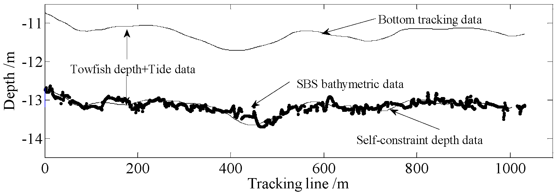
In the above preprocessing, the bottom tracking is very important to obtain towfish height and the initial seabed topography. In Figure 6a, it can be found that the blank area or water column area differs distinctly from the seabed areas in gray levels. According to the characteristic, the bottom tracking can be carried out. For a ping of Strip I as shown in Figure 7a, the gray level sequence is firstly extracted as shown in Figure 7b. Then, to calculate the gray level differences of any two adjacent echoes and find the maximum difference by Equation (15), the seabottom point can be detected as shown in Figure 7c, and the towfish height can be computed by Equation (16). To detect the seabottom points in other pings, the sequence of along-track towfish heights is obtained as shown in Figure 8. To avoid the effect of the water-column noise, the bottom tracking is smoothed by moving averaging for every 20 pings. Comparing sequences of the towfish heights and the corresponding seabed heights from bathymetric data, as shown in Figure 8, a strong similarity can be found between them except the various biases caused by the variations of tidal levels and towfish depths. Using the towfish heights, the slant-range correction can be performed and this is shown in Figure 6c. By geocoding, the image is obtained as shown in Figure 6d and it will be used to reconstruct the seabed topography. By combining the towfish heights, towfish depths and tidal levels, the along-track seabed height sequence is obtained and shown in Figure 8. It can be seen that the seabed height has high consistency with that from the SBS bathymetric data. Comparing the two sets of seabed heights, the statistic parameters of the biases are listed in Table 1, which shows that the along-track depth data achieved by the proposed method has the standard deviation of 0.13 m and can be used to build the initial seabed topography.
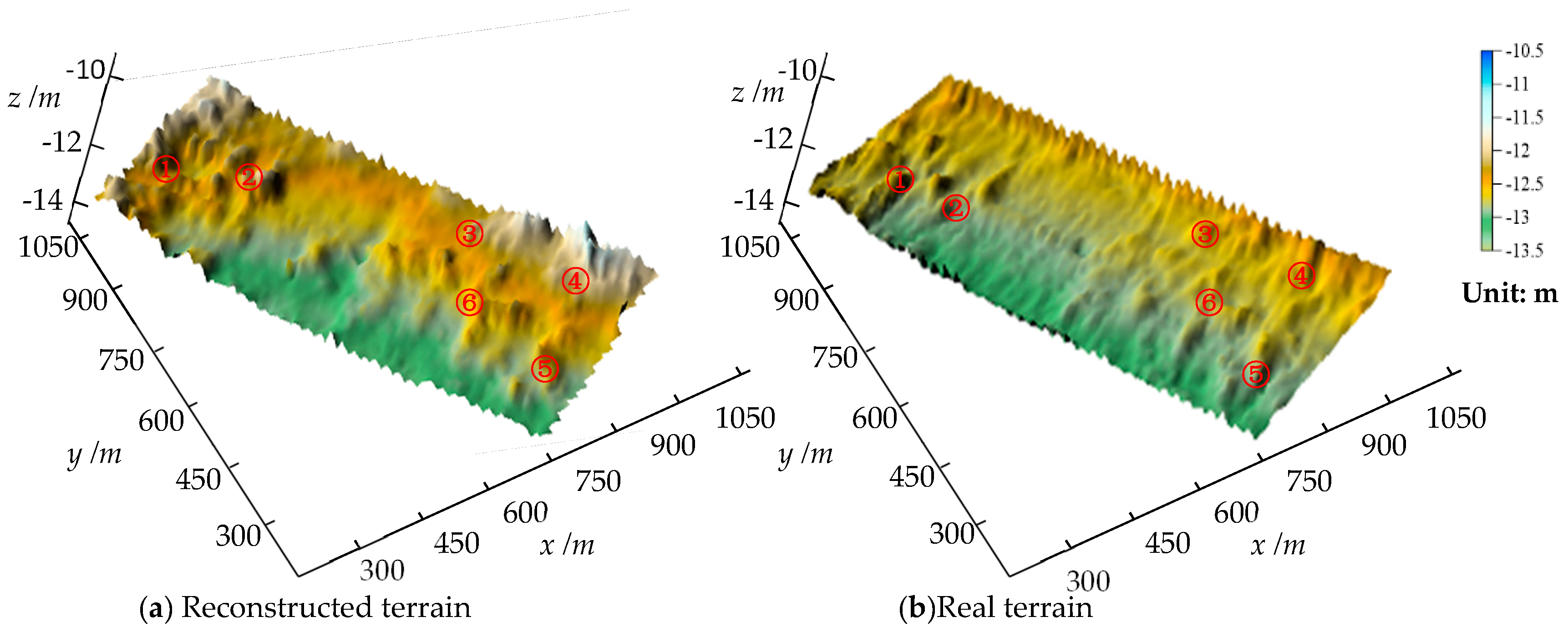
The similar process is used for Strip II and III, the sequences of along-track seabed heights are obtained and the seabed DEM can be established by a linear interpolation. The DEM as shown in Figure 9 will be used as the initial seabed topography in the reconstruction of Strip I. Using the initial seabed topography shown in Figure 9 as self-constraint, the seabed topography is reconstructed from the image as shown in Figure 6d by the process depicted in Figure 4. The reconstruction result is shown in Figure 10a. The reconstructed terrain grid size is 0.6 m × 0.6 m, which is the same as the image pixel resolution representing the actual. The resolution of terrain grid data is improved significantly relative to the bathymetric terrain with terrain grid size of 40 m × 40 m. It can be seen that the topography vividly presents the six features as shown in Figure 6d.
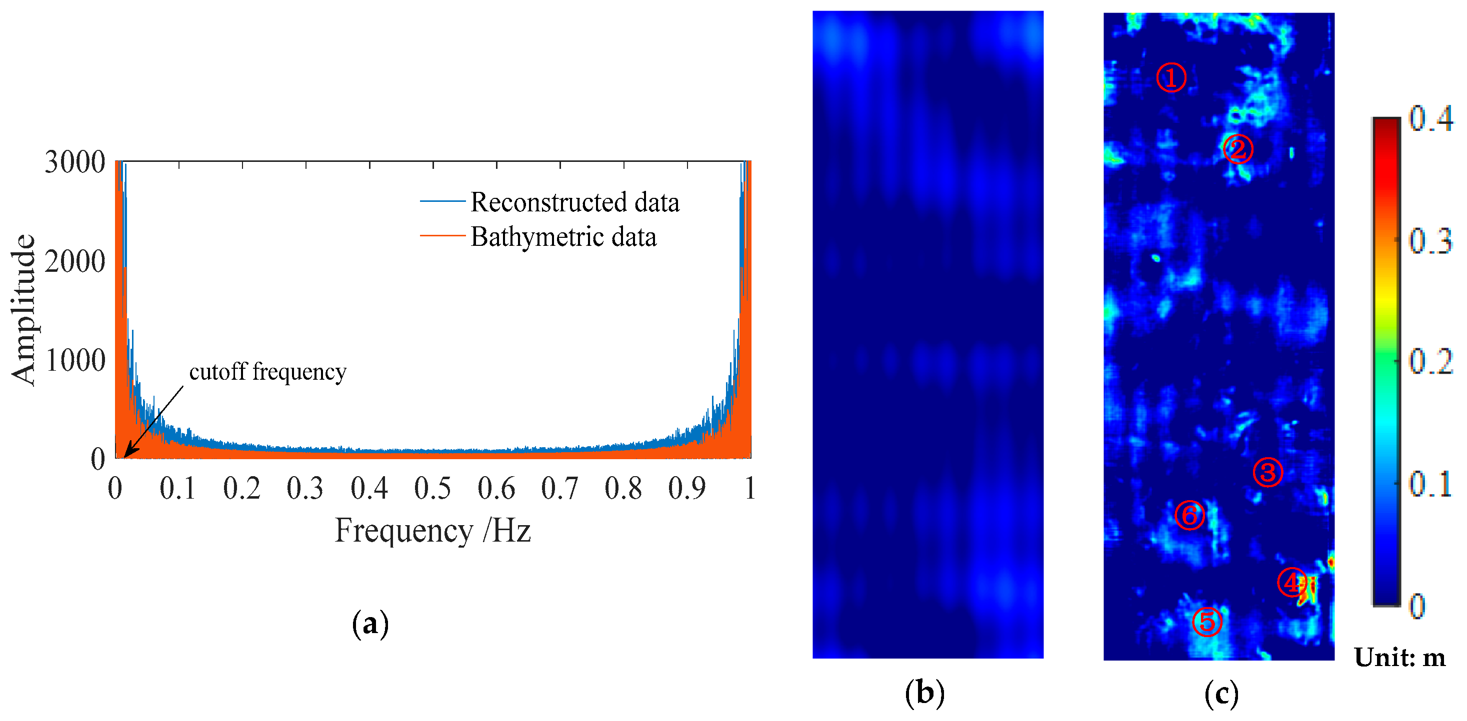
For convenient comparison, an interpolation is performed for the SBS bathymetric data to get the same data resolution as that of the reconstructed topography. Two DEMs in Figure 10 are established by using the reconstruction data and the interpolated bathymetric data. Taking the bathymetric DEM as reference, the reconstructed DEM in Figure 10a has high similarity with the bathymetric one in Figure 10b on the whole trend, but reflects more refined seabed features. To assess the capability of the reconstruction in reflecting microtopography, frequency analysis is adopted for the two DEMs. The amplitude-frequency curves are shown in Figure 11a. It can be seen that the reconstruction has higher amplitude than the bathymetric data at every frequency, especially at mid-high frequency band. The amplitude-frequency curves show that the reconstruction has better performance in reflecting the microtopography. According to variations of the two curves, the cut-off frequency as 0.02 Hz (Figure 11a) is chosen for dividing the DEMs into high-frequency and low-frequency parts. The high-frequency part and low-frequency part differences of two DEMs are shown in Figure 11b,c. It can be seen that the low-frequency part differences are less than 0.1 m and the high-frequency differences vary mainly between 0.0–0.2 m and then between 0.2–0.4 m at some specific positions, which shows that the reconstructed DEM has consistent terrain tendency with the bathymetric one and can reflect the seabed features with the height more than 0.2 m at least.
To assess the accuracy of reconstruction, the external bathymetric data is used as a reference, and the biases of the reconstructed seabed topography at these bathymetric points are calculated. The statistical results of the biases are listed in Table 2. It can be seen that the maximum, minimum, mean and standard deviation of the biases are 0.30 m, −0.43 m, 0.00 m and 0.12 m and the proportion of absolute biases less than 0.30 m is 99.22%. The reconstruction achieves nearly the same accuracy as the bathymetric data. According to the reconstruction accuracy and the ability to reflect small-size terrain features, the reconstruction can reflect the seabed feature with the height more than 0.2 m at least and achieve the standard deviation better than 0.15 m.
To analyze how the reconstruction accuracies vary with the across-track distances, the bathymetric data of the eight SBS surveying lines symmetrically distributed on both sides of the SSS towfish tracking line in Figure 12a are used as the reference to assess the reconstruction accuracies at the 8 lines. The reconstruction errors at these 8 lines are calculated and the statistical parameters and PDF curves of the biases are shown in Table 3 and Figure 12b.
It can be seen from Figure 12 and Table 3 that the variation ranges and standard deviations of reconstruction biases at different across-track distance lines are closed to those shown in Table 2, but the systematic biases appear in the reconstruction results of line 1 and 8 because the corresponding mean biases are respectively 0.12 m and 0.10 m. The problem appearing at the outmost across-track locations may be induced by imperfect radiometric distortion correction and is discussed in Section 5.2.
4.3. Seabed Topography Reconstruction of Surveying Area
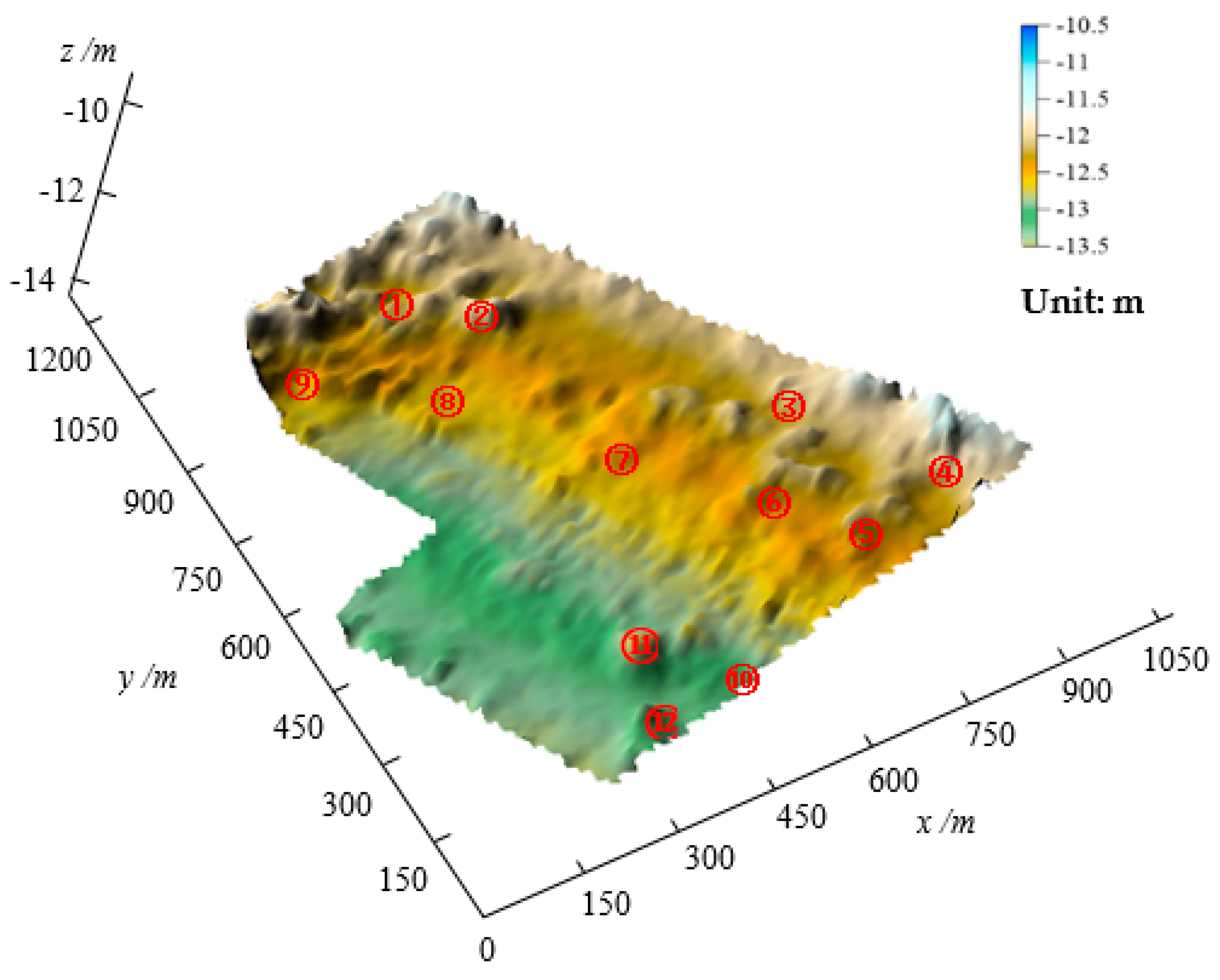
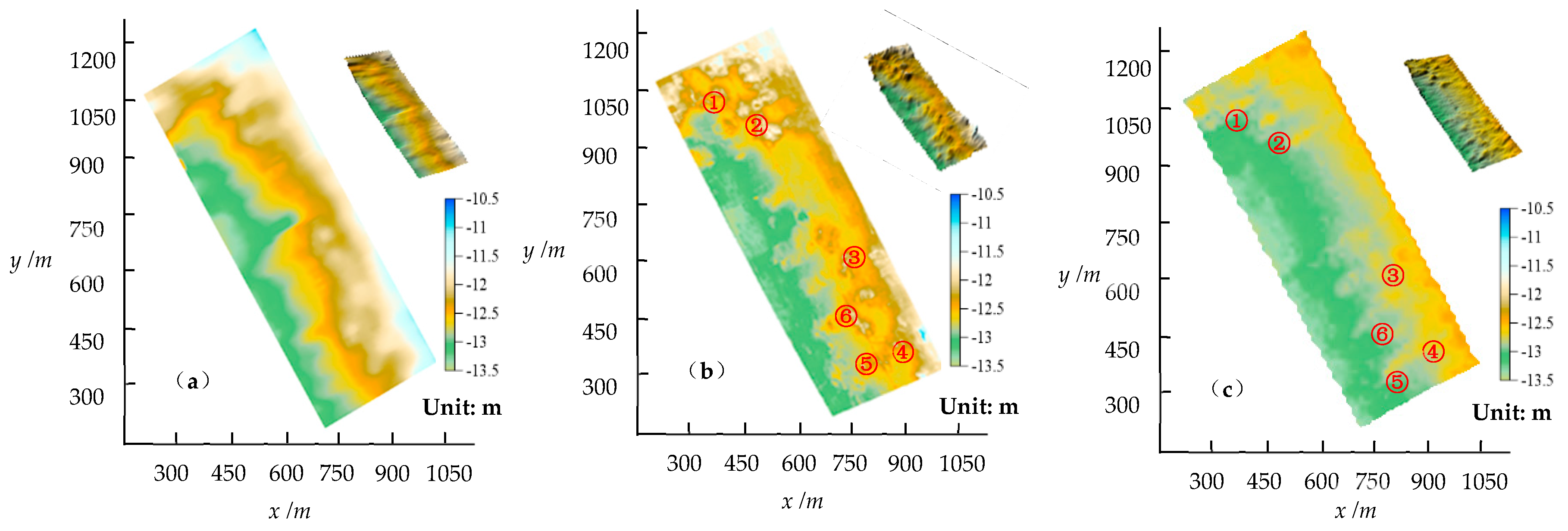
Using a similar method and process to that depicted in Section 4.2, the seabed topographies of Strip II and III are reconstructed. Combining the reconstruction results of three strips, the seabed DEM of the surveying area is established and shown in Figure 13. Compared with the DEM as shown in Figure 5b, the reconstructed topography shows good consistence with the real one. However, because of the resolution difference of the SSS image (0.6 m) and the SBS bathymetric data (40 m), the reconstruction improves the topography resolution about 66 times and reflects clearer seabed features relative to the real DEM. Besides the seabed features ①–⑫ in Figure 5, some micro features are also displayed in Figure 13.
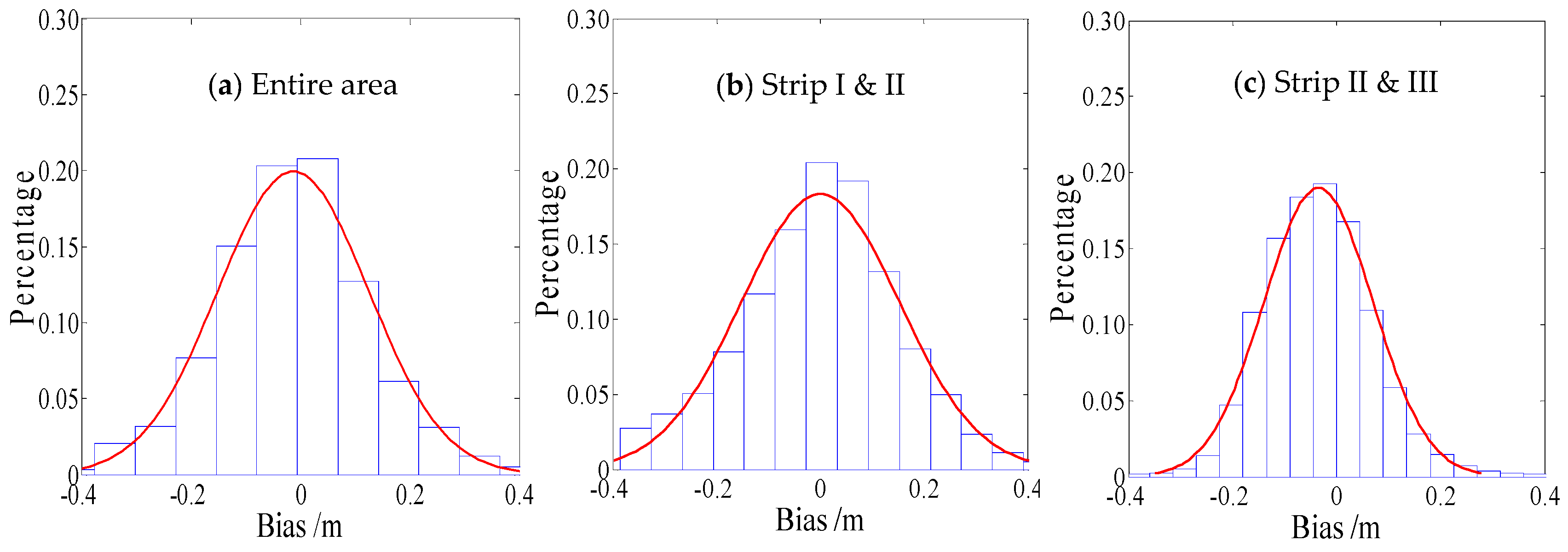
To assess the accuracy in the surveying area, the biases between the whole reconstruction topography and the bathymetric data are calculated, and the statistical results and PDF curves of the reconstruction biases are shown in Table 4 and Figure 14a. Compared with Table 2, the reconstruction accuracy in the area is close to that of Strip I. The results show the proposed method has good applicability and consistent accuracy in the reconstruction. Using Strip II and III, the proposed method can also be evaluated in terms of the reconstruction consistency of the overlapping area of adjacent strips. Comparing topography differences of the overlapping area, the statistical results of these biases are shown in Table 4 and the corresponding PDF curves are shown in Figure 14b,c. It can be seen that the biases obey the normal standard distribution and the proportion of the absolute biases less than 0.3 m is 98.66%. Statistical results prove that the reconstruction of the overlapping area between adjacent strips is consistent.
The same phenomenon that some big biases exist in the reconstruction of Strip I also happens in other strips. The reason for this could be attributed to the abnormal bottom tracking and the image noise caused by the water environment. Nonetheless, the statistical results in Table 4 show that the proposed method achieves the standard deviation less than 0.15 m, and has consistent accuracy in the reconstructions of all SSS strips.
5. Discussion
5.1. Noise in SSS Image
The proposed method reconstructs the seabed topography from SSS images with a self-constraint. Once the SSS transducer receives abnormal echoes from fish, suspended solids or particles in the water column, abnormal features or noise will be formed in the SSS image [9,35] and this will result in abnormal topography reconstruction. The problem can be avoided by filtering the SSS image and the reconstructed topography. By obeying discrete distribution, the noise in the SSS image can be easily removed by an average filtering or the threshold filtering. In the threshold filtering, the pixel whose gray level difference is more than 10 away from its surrounding pixels will be filtered. Although most noise can be removed from the SSS image, some residual noise still remains and is reflected in the reconstructed terrain. The noise from the suspended solids has strong backscatter strengths. Thus, the reconstruction of the noise will differ obviously from those of its surrounding terrain and can be removed by the topographic trend filtering [7].
5.2. Eeffects of Refraction of Waves, Towfish Depth and Cross-Track Distance
5.2.1. Refraction of Waves in the Water Column
In general, in SSS image processing, the refraction of the wave is ignored and the sound ray is regarded as a straight line for the calculation of echo position in a ping measurement, which results in inaccurate target position in a SSS image. To weaken the effect, the sound ray tracing is added in the reconstruction process (2) of Section 3.4.
In the sound ray tracing, two parameters, the propagation time and incident angle of an echo are required. The propagation time can be obtained by the equal-interval time sampling in a ping measurement. The incident angle can be approximately estimated by the towfish height and the across-track distance of the echo. After the sound ray tracing, the positions of the echoes or seabed features in SSS image can be determined accurately.
5.2.2. Towfish Depth and Across-Track Distance
The footprint of a beam varies with towfish depth and across-track distance. The larger the towfish depth and the across-track distance, the smaller the backscatter intensities are. This phenomenon leads to the disequilibrium of gray level in the SSS image and the inaccurate presentation of sediment reflectivity as well as the incorrect reconstruction of seabed topography. The problem can be solved by the radiometric distortion correction and the slant distance correction [29,30,31]. The radiometric distortion correction can remove the effects of towfish depth change. The integration of the slant distance correction and radiometric distortion correction can weaken the effect of various across-track distances. After these corrections, the quality of the SSS image is improved (Figure 6) relative to the raw waterfall image. Using the improved SSS image to reconstruct seabed topography, nearly consistent accuracies were obtained in different across-track distances (Figure 12, Table 3). We can also find slight accuracy decreases with the increase of the across-track distances, which shows that the effects of towfish depth and across-track distance were not removed completely by the radiometric distortion correction used in this paper and needs to be weakened by further improving the model.
5.3. Seabed Sediments
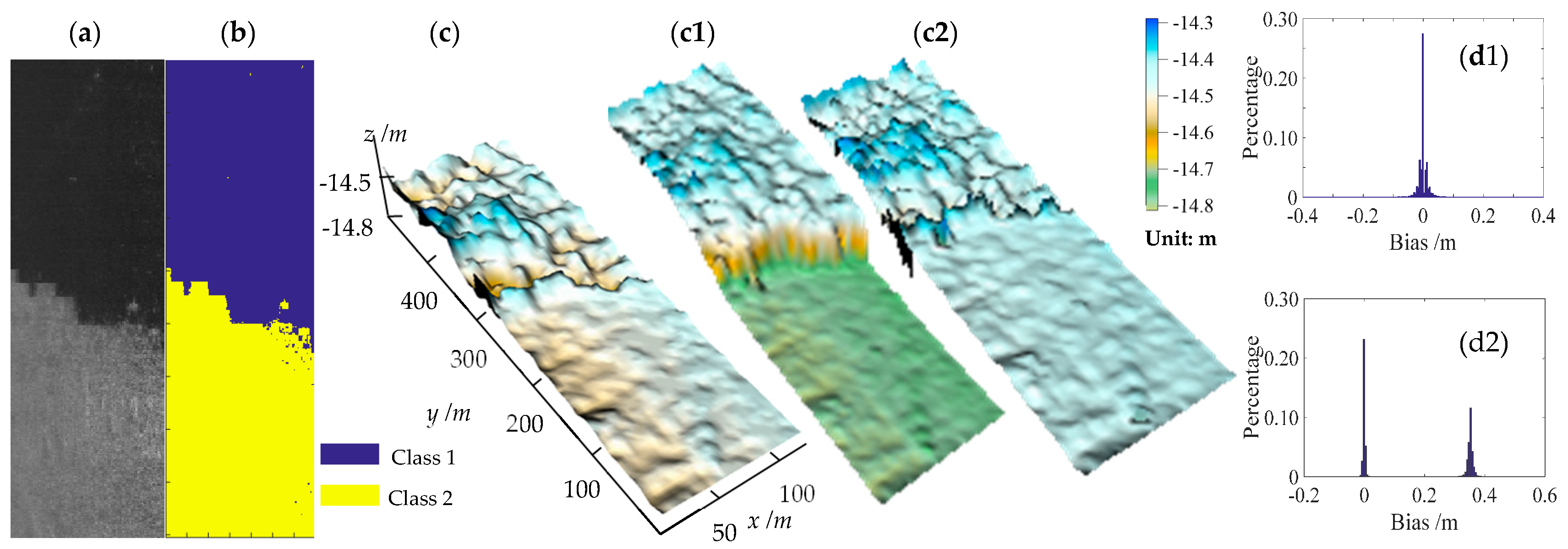
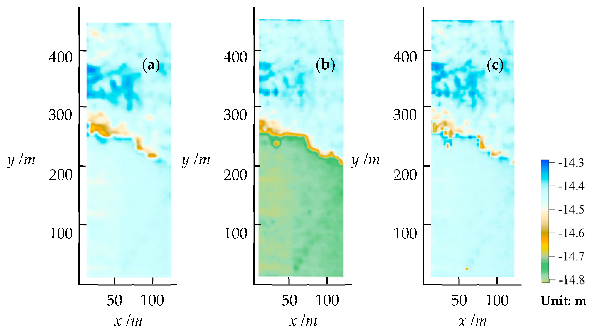
According to Section 2, the gray level of a pixel in the SSS image or the backscatter strength of a beam footprint is related to the seabed sediment and topographic variation. Because the experimental area is of homogeneous sediment, the SSS images only reflect the variation of seabed topography, and thus the impacts of seabed sediments on the reconstruction are ignored. The above experiments have verified that the reconstruction has good results under the situation of homogeneous seabed sediment. For further applications of the proposed method in inhomogeneous areas, the sediment variations need to be considered. The inhomogeneous sediments have different acoustic impedances and reflectivity albedos [38], which affects the backscatter intensities (Figure 15a) and the reconstruction by Equation (2). If the effect is ignored, the reconstruction will result in a systematic bias in the reconstructed topographies of two different sediment areas due to using the same reflectivity albedo (Figure 15(c1,d1)). To remove the impacts of sediment variations on the reconstruction, an unsupervised classification on the SSS images [31,39] or the sediment sampling [38,40] in the reconstructed area needs to be implemented before the reconstruction. To some extent, the unsupervised classification may provide a convenient way to obtain approximate distributions of different sediments in the area [31]. According to the classifications, the SSS image is divided into several parts (Figure 15b). In the separated homogeneous sediment areas, the reconstructions of seabed topographies are carried out by the proposed method. As shown in Equation (3), the seabed shape is obtained by the normalized intensity Inorm in this paper, and a given constant reflectivity albedo u will not bring effect on the reconstruction of the homogeneous sediment seabed areas. Therefore, the entire seabed topography (Figure 15(c2)) is finally obtained by combining the reconstructed seabed topographies of different sediment areas. Compared with the bathymetric topography (Figure 15c), the reconstruction by considering the sediment variations (Figure 15(c2)) achieved higher accuracy (mean bias of 0.01 m, standard bias of 0.06 m, Figure 15(d2)) than that by ignoring the variations (mean bias of 0.17 m, standard bias of 0.21 m, Figure 15(d1)).
5.4. Bottom Tracking and Initial Seabed Topography
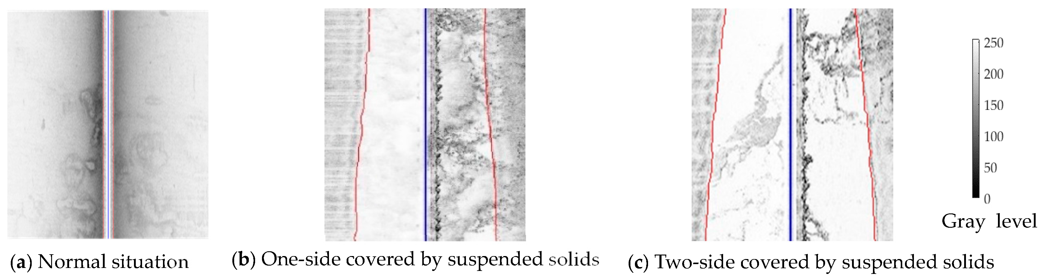
The initial topography is used as the constraint of reconstructing absolute topography in the proposed method. Without the constraint, the proposed method can only get the relative topographic variations [19]. Relative to the existing methods [15,16,17,18,19,20,21,22], the proposed method obtains the initial topography by bottom tracking from SSS waterfall images, but not the external bathymetric data. Therefore, the constraint is named self-constraint in this paper. Being affected by the suspended solids in the water column, the bottom tracking may be affected and this results in inaccurate towfish height tracked by the mutation of gray levels depicted in Section 3.2. Under the situations as shown in Figure 16, the symmetric principle, namely the detected port towfish height equals the starboard one and the continuous seabed variation principle are used for diagnosing and repairing the abnormal [35]. If one side of the water column is covered by suspended solids, the detected towfish height of the covered side will be replaced by that of the uncovered one (Figure 16b). If the two sides are both covered, the abnormal towfish height can be repaired by interpolating correct ones of its neighbor pings (Figure 16c).
5.5. Determination of Iteration Termination Threshold
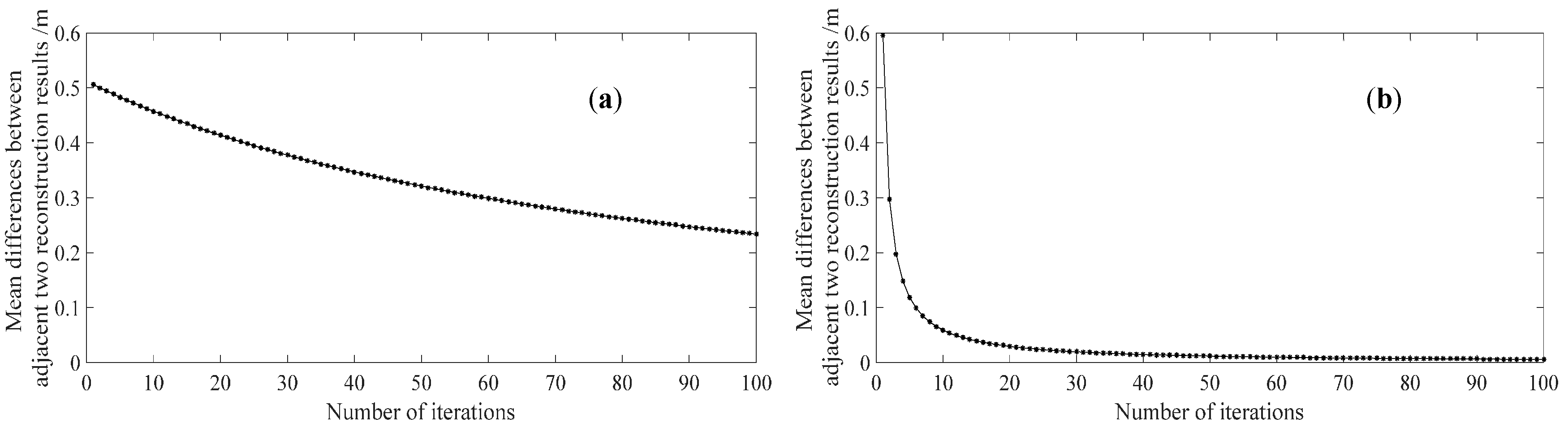
In the reconstruction, Equation (13) is solved by an iteration operation. As shown in Equation (14), the iteration operation is performed using an initial z0 and stopped by a given threshold ε. It is well known that the Netwon method converges to a stable result when an accurate starting value is known [32,33]. To analyze the importance of initial terrain in the iteration, an inappropriate initial terrain and an appropriate one are respectively used for the iteration and the corresponding convergence curves are shown in Figure 17a,b. It can be seen that the curve converges difficultly to a stable value within finite iterations when an inappropriate initial terrain is provided. Reversely, the curve easily reaches a stable result after the 42nd iteration when an appropriate initial terrain is given. This experiment demonstrates that it is better to provide an appropriate initial terrain in the iteration. The method of how to get the initial terrain is depicted in Section 3.2. Figure 17b displays the iteration from unstable to stable changes, which implies that the difference of adjacent iterations corresponding to the inflection point of the convergence curve can be set as ε. In the experiments depicted in Section 4, ε is set as 0.05 m. Similarly, the method for determining ε can also be used for the other seabed topography reconstructions from SSS images.
6. Conclusions
This study proposes a new method to reconstruct detailed seabed topography from side-scan sonar image with self-constraint. Without the need of external bathymetric data, the self-constraint or the initial topography, which is approximate to the real one, is formed by combining the towfish height from bottom tracking, towfish depth from built-in pressure sensor and tide level obtained from the SSS measurement. Therefore, the robustness of the reconstruction is improved and the reconstruction work is significantly simplified. Besides, the effects of sediment variations can be weakened by the unsupervised classification. The quality of the SSS image that is influenced by noise, suspended bodies, refraction of wave in water and the cross-track distance etc. can be improved by SSS image preprocessing. As a result, the accuracy of the reconstruction is improved. These conclusions were proved by the experiments. In the experiments, the reconstructed seabed topography reflected refined micro-terrain features and achieved the standard deviation less than 0.15 m. Moreover, the resolution of the reconstructed topography is about 66 times higher than that of the real one.
The propose method, which provides an approach to get detailed seabed topography from the high-resolution SSS image, is a supplement but not substitution for the existing bathymetric methods, and the proposed method has wide applications in obtaining fine seabed topography, especially in deep waters.
Acknowledgments
This research is supported by the National Natural Science Foundation of China (Coded by 41576107, 41376109 and 41176068) and the National Science and Technology Major Project (Coded by 2016YFB0501703). The data used in this study were provided by the Guangzhou Marine Geological Survey Bureau. The authors are grateful for their support.
Author Contributions
Jianhu Zhao, Xiaodong Shang and Hongmei Zhang developed and designed the experiments; Jianhu Zhao and Xiaodong Shang performed the experiments; Jianhu Zhao, Xiaodong Shang and Hongmei Zhang analyzed the data; Jianhu Zhao, Xiaodong Shang and Hongmei Zhang wrote the paper.
Conflicts of Interest
The authors declare no conflict of interest.
Appendix A
The 2D colored images of the DEM (Figure 5b) and the reconstructed topography (Figure 13) are respectively presented in Figure A1a,b.
Figure A1.
The 2D colored images of the seabed DEM constructed by dense SBS bathymetric data (a) and the reconstructed topography from the SSS images (b). ①–⑫ denote the seabed features as the same as those in Figure 5.
Figure A1.
The 2D colored images of the seabed DEM constructed by dense SBS bathymetric data (a) and the reconstructed topography from the SSS images (b). ①–⑫ denote the seabed features as the same as those in Figure 5.
The 2D colored images of the initial topography of Strip I (Figure 9), the reconstructed topography (Figure 10a) and the real terrain constructed by SBS bathymetric data (Figure 10b) are respectively presented in Figure A2a–c.
Figure A2.
The 2D colored images of the initial topography (a), the reconstructed topography (b) and real terrain constructed by SBS bathymetric data (c) of Strip I. ①–⑥ denote the topographic features in Strip I.
Figure A2.
The 2D colored images of the initial topography (a), the reconstructed topography (b) and real terrain constructed by SBS bathymetric data (c) of Strip I. ①–⑥ denote the topographic features in Strip I.

The 2D colored images of the actual bathymetric topography (Figure 15c), the reconstructed topographies by ignoring and considering the effects of sediment variations (Figure 15(c1,c2)) are respectively presented in Figure A3a–c.
Figure A3.
The 2D colored images of the actual bathymetric topography (a), the reconstructed topographies by ignoring (b) and considering (c) the effects of sediment variations.
Figure A3.
The 2D colored images of the actual bathymetric topography (a), the reconstructed topographies by ignoring (b) and considering (c) the effects of sediment variations.

References
- Sharma, R.; Khadge, N.H.; Jai Sankar, S. Assessing the distribution and abundance of seabed minerals from seafloor photographic data in the Central Indian Ocean Basin. Int. J. Remote Sens. 2013, 34, 1691–1706. [Google Scholar] [CrossRef]
- Fakiris, E.; Papatheodorou, G.; Geraga, M.; Ferentinos, G. An automatic target detection algorithm for swath sonar backscatter imagery, using image texture and independent component analysis. Remote Sens. 2016, 8, 373. [Google Scholar] [CrossRef]
- Hasan, R.; Ierodiaconou, D.; Monk, J. Evaluation of four supervised learning methods for benthic habitat mapping using backscatter from multi-beam sonar. Remote Sens. 2012, 4, 3427. [Google Scholar] [CrossRef]
- Powers, J.; Brewer, S.K.; Long, J.M.; Campbell, T. Evaluating the use of side-scan sonar for detecting freshwater mussel beds in turbid river environments. Hydrobiologia 2015, 743, 127–137. [Google Scholar] [CrossRef]
- Hernández, J.D.; Istenič, K.; Gracias, N.; Palomeras, N.; Campos, R.; Vidal, E.; García, R.; Carreras, M. Autonomous underwater navigation and optical mapping in unknown natural environments. Sensors 2016, 16, 1174. [Google Scholar] [CrossRef] [PubMed]
- Diaz, J.V.M. Analysis of Multibeam Sonar Data for the Characterization of Seafloor Habitats. Master’s Thesis, The University of New Brunswick, Fredericton & Saint John, NB, Canada, 2000. [Google Scholar]
- Zhao, J.; Yan, J.; Zhang, H.; Zhang, Y.; Wang, A. A new method for weakening the combined effect of residual errors on multibeam bathymetric data. Mar. Geophys. Res. 2014, 35, 379–394. [Google Scholar] [CrossRef]
- Canepa, G.; Bergem, O.; Pace, N.G. A new algorithm for automatic processing of bathymetric data. IEEE J. Ocean. Eng. 2003, 28, 62–77. [Google Scholar] [CrossRef]
- Blondel, P. The Handbook of Sidescan Sonar; Springer: Berlin/Heidelberg, Germany; New York, NY, USA, 2009; pp. 35–77. ISBN 978-3-540-42641-7. [Google Scholar]
- Trucco, E.; Petillot, Y.R.; Ruiz, I.T.; Plakas, K.; Lane, D.M. Feature tracking in video and sonar subsea sequences with applications. Comput. Vis. Image Underst. 2000, 79, 92–122. [Google Scholar] [CrossRef]
- Horn, B.K.P. Shape from Shading: A Method for Obtaining the Shape of a Smooth Opaque Object from One View. Ph.D. Thesis, Massachusetts Institute of Technology, Cambridge, MA, USA, 1970. [Google Scholar]
- Zhang, R.; Tsai, P.S.; Cryer, J.E.; Shah, M. Shape from shading: A survey. IEEE Trans. Pattern Anal. Mach. Intell. 1999, 21, 690–706. [Google Scholar] [CrossRef]
- Ragheb, H.; Hancock, E.R. Surface radiance correction for shape from shading. Pattern Recognit. 2005, 38, 1574–1595. [Google Scholar] [CrossRef]
- Bell, J.M.; Chantler, M.J.; Wittig, T. Sidescan sonar: A directional filter of seabed texture? IEE Proc. Radar Sonar Navig. 1999, 146, 65–72. [Google Scholar] [CrossRef]
- Johnson, A.E. Incorporating different reflection models into surface reconstruction. In Proceedings of the Unmanned Untethered Submersible Technology Conference, Durham, UK, 27–29 September 1993; pp. 446–459. [Google Scholar]
- Johnson, A.E.; Hebert, M. Seafloor map generation for autonomous underwater vehicle navigation. Auton. Robot. 1996, 3, 145–168. [Google Scholar] [CrossRef]
- Langer, D.; Hebert, M. Building qualitative elevation maps from side scan sonar data for autonomous underwater navigation. In Proceedings of the IEEE International Conference on Robotics and Automation, Sacramento, CA, USA, 9–11 April 1991. [Google Scholar]
- Bikonis, K.; Moszynski, M.; Lubniewski, Z. Application of shape from shading technique for side scan sonar images. Pol. Marit. Res. 2013, 20, 39–44. [Google Scholar] [CrossRef]
- Zhao, J.; Shang, X.; Zhang, H. Recovering seabed topography from sonar image with constraint of sounding data. J. China Univ. Min. Technol. 2017, 46, 443–448. [Google Scholar] [CrossRef]
- Wang, A.; Zhao, J.; Shang, X.; Zhang, H. Recovery of seabed 3D micro-topography from side-scan sonar image constrained by single-beam soundings. J. Harbin Eng. Univ. 2017, 38, 739–745. [Google Scholar] [CrossRef]
- Dura, E.; Bell, J.; Lane, D. Reconstruction of textured seafloors from side-scan sonar images. IEE Proc. Radar Sonar Navig. 2004, 151, 114–126. [Google Scholar] [CrossRef]
- Coiras, E.; Petillot, Y.; Lane, D.M. Multiresolution 3-d reconstruction from side-scan sonar images. IEEE Trans. Image Process. 2007, 16, 382–390. [Google Scholar] [CrossRef] [PubMed]
- Eckart, C. Principles of Underwater Sound, 3rd ed.; McGraw-Hill: New York, NY, USA, 1983; pp. 252–253. ISBN 0070660875. [Google Scholar]
- Jackson, D.R.; Winebrenner, D.P.; Ishimaru, A. Application of the composite roughness model to high-frequency bottom backscattering. J. Acoust. Soc. Am. 1986, 79, 1410–1422. [Google Scholar] [CrossRef]
- Bell, J.M.; Linnett, L.M. Simulation and analysis of synthetic sidescan sonar images. IEE Proc. Radar Sonar Navig. 1997, 144, 219–226. [Google Scholar] [CrossRef]
- Gensane, M. A statistical study of acoustic signals backscattered from the sea bottom. IEEE J. Ocean. Eng. 2002, 14, 84–93. [Google Scholar] [CrossRef]
- Chang, Y.C.; Hsu, S.K.; Tsai, C.H. Sidescan sonar image processing: Correcting brightness variation and patching gaps. J. Mar. Sci. Technol. 2010, 18, 785–789. [Google Scholar]
- Ronald, W.; Marwood, N. Electro-Optics Handbook; McGraw-Hill: New York, NY, USA, 2000; ISBN 0-07-068716-1. [Google Scholar]
- Cervenka, P.; Moustier, C.D. Sidescan sonar image processing techniques. IEEE J. Ocean. Eng. 1993, 18, 108–122. [Google Scholar] [CrossRef]
- Chavez, P.S., Jr.; Isbrecht, J.A.; Galanis, P.; Gabel, G.L.; Sides, S.C.; Soltesz, D.L.; Ross, S.L.; Velasco, M.G. Processing, mosaicking and management of the monterey bay digital sidescan-sonar images. Mar. Geol. 2002, 181, 305–315. [Google Scholar] [CrossRef]
- Zhao, J.; Yan, J.; Zhang, H.; Meng, J. A new radiometric correction method for side-scan sonar images in consideration of seabed sediment variation. Remote Sens. 2017, 9, 575. [Google Scholar] [CrossRef]
- Ping-Sing, T.; Shah, M. Shape from shading using linear approximation. Image Vis. Comput. 1994, 12, 487–498. [Google Scholar] [CrossRef]
- John, H.M.; Kurtis, D.F. Numerical Methods Using MATLAB, 4th ed.; Publishing House of Electronics Industry: Beijing, China, 2017; pp. 136–138. ISBN 9787121314995. [Google Scholar]
- Reed, S.; Tena, R.I.; Capus, C.; Petillot, Y. The fusion of large scale classified side-scan sonar image mosaics. IEEE Trans. Image Process. 2006, 15, 2049–2060. [Google Scholar] [CrossRef] [PubMed]
- Zhao, J.; Wang, X.; Zhang, H.; Wang, A. A comprehensive bottom-tracking method for sidescan sonar image influenced by complicated measuring environment. IEEE J. Ocean. Eng. 2017, 42, 619–631. [Google Scholar] [CrossRef]
- Zhao, J.; Zhang, H.; John, E.H. Determination of precise instantaneous tidal level at vessel. Geomat. Inf. Sci. Wuhan Univ. 2006, 31, 1067–1070. [Google Scholar] [CrossRef]
- Zhao, J.; Zhang, H.; Chen, Z.; Wang, Z.; Zhang, Y.; Shang, X. On-the-fly measurements of large-drop water level and high flow velocity in the closure gap. Flow Meas. Instrum. 2015, 45, 198–206. [Google Scholar] [CrossRef]
- Mohamed, S.; Mostafa, R. Seabed sub-bottom sediment classification using parametric sub-bottom profiler. NRIAG J. Astron. Geophys. 2016, 5, 87–95. [Google Scholar] [CrossRef]
- Arthur, D.; Vassilvitskii, S. K-means++: The advantages of careful seeding. In Proceedings of the Advances in the Eighteenth Annual ACM-SIAM Symposium on Discrete Algorithms, New Orleans, LA, USA, 7–9 January 2007; Society for Industrial and Applied Mathematics: Philadelphia, PA, USA, 2007; pp. 1027–1035. [Google Scholar]
- Pinson, L.J.; Henstock, T.J.; Dix, J.K.; Bull, J.M. Estimating quality factor and mean grain size of sediments from high-resolution marine seismic data. Geophysics 2008, 73, 19–28. [Google Scholar] [CrossRef]
Figure 1.
Scattering model on seabed. Ei, Es and Ef are the incident acoustic energy, BS and specular reflection energy, θ and δ are the incident and grazing angle, and dS is the area of beam footprint.
Figure 1.
Scattering model on seabed. Ei, Es and Ef are the incident acoustic energy, BS and specular reflection energy, θ and δ are the incident and grazing angle, and dS is the area of beam footprint.
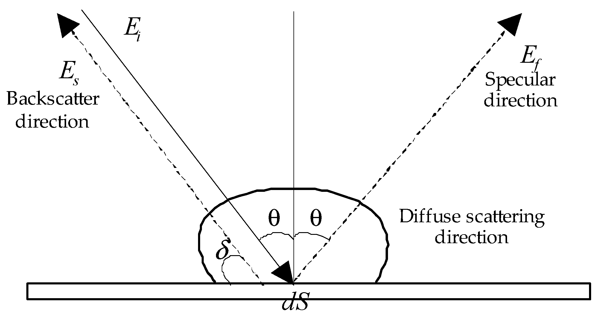
Figure 2.
SSS measurement and acoustic wave reflection on seabed. hx is the towfish height, denotes the incident vector, denotes the seabed surface normal vector of a point g, θxy denotes the incident angle on seabed, ϕxy denotes the angle between the incident and the vertical directions.
Figure 2.
SSS measurement and acoustic wave reflection on seabed. hx is the towfish height, denotes the incident vector, denotes the seabed surface normal vector of a point g, θxy denotes the incident angle on seabed, ϕxy denotes the angle between the incident and the vertical directions.

Figure 3.
Flow diagram of obtaining initial seabed topography or the self-constraint.
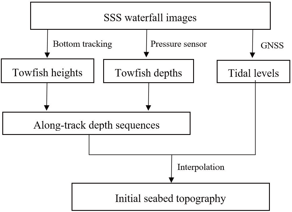
Figure 4.
Flow diagram of reconstructing topography from SSS image.

Figure 5.
SSS image (a) and seabed DEM constructed by dense SBS bathymetric data (b) in the measurement area. ①–⑫ denote the seabed topographic features.
Figure 5.
SSS image (a) and seabed DEM constructed by dense SBS bathymetric data (b) in the measurement area. ①–⑫ denote the seabed topographic features.

Figure 6.
SSS image preprocessing of Strip I. ①–⑥ denote the seabed features corresponding to those in Figure 5a. (a) Waterfall image; (b) Radiation correction; (c) Slant-range correction; (d) Geocoding image.
Figure 6.
SSS image preprocessing of Strip I. ①–⑥ denote the seabed features corresponding to those in Figure 5a. (a) Waterfall image; (b) Radiation correction; (c) Slant-range correction; (d) Geocoding image.
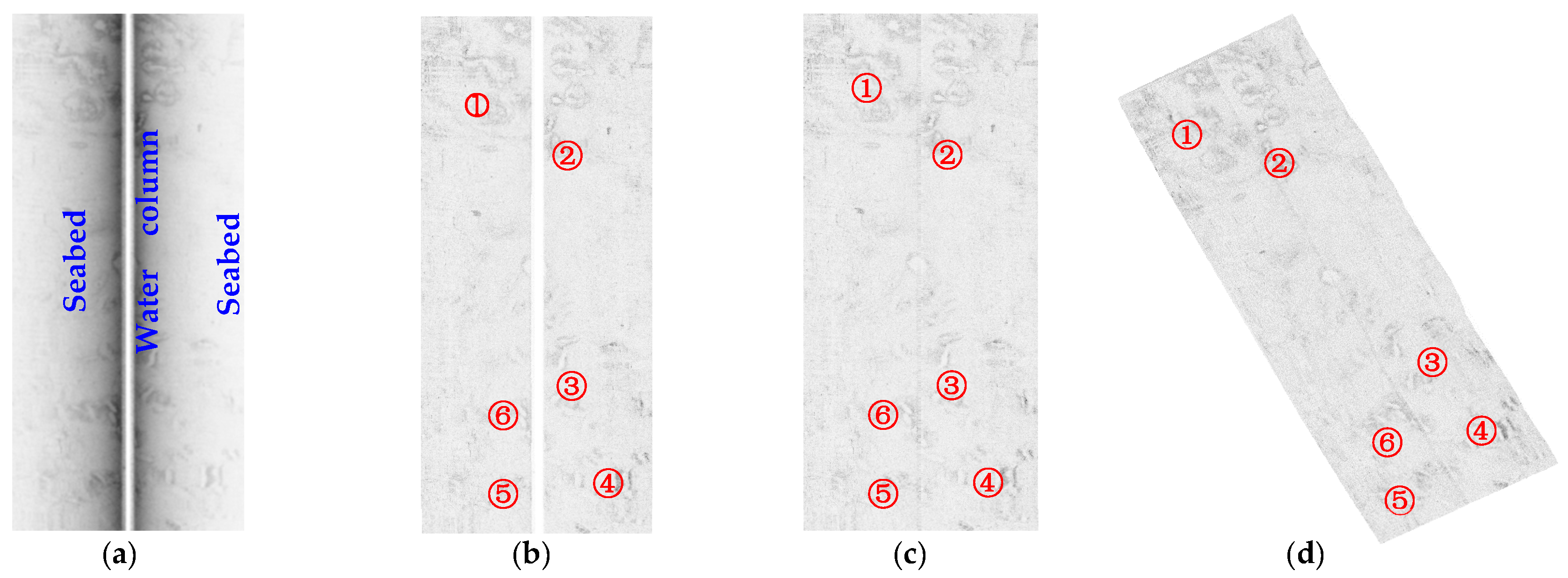
Figure 7.
Bottom tracking and acquisition of towfish height. The red lines and the blue line in (a) respectively denote the seabottom lines and a ping scanning line. (a) Waterfall image; (b) Gray level sequence of the ping; (c) Gray level difference sequence of the ping.
Figure 7.
Bottom tracking and acquisition of towfish height. The red lines and the blue line in (a) respectively denote the seabottom lines and a ping scanning line. (a) Waterfall image; (b) Gray level sequence of the ping; (c) Gray level difference sequence of the ping.
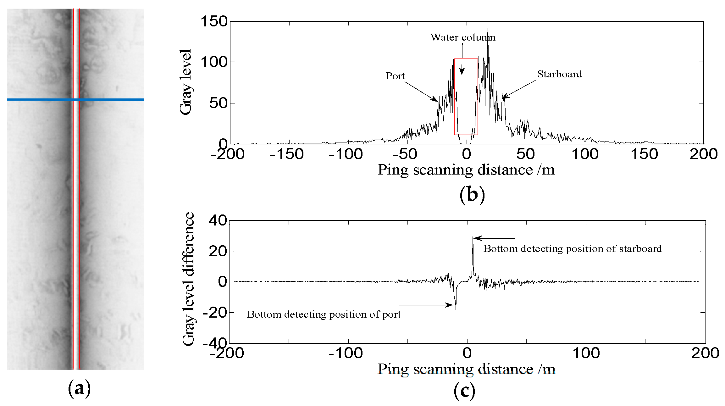
Figure 8.
Sequences of the towfish heights from the bottom tracking, the self-constraint data and the SBS bathymetric data.
Figure 8.
Sequences of the towfish heights from the bottom tracking, the self-constraint data and the SBS bathymetric data.

Figure 9.
Initial topography of Strip I.
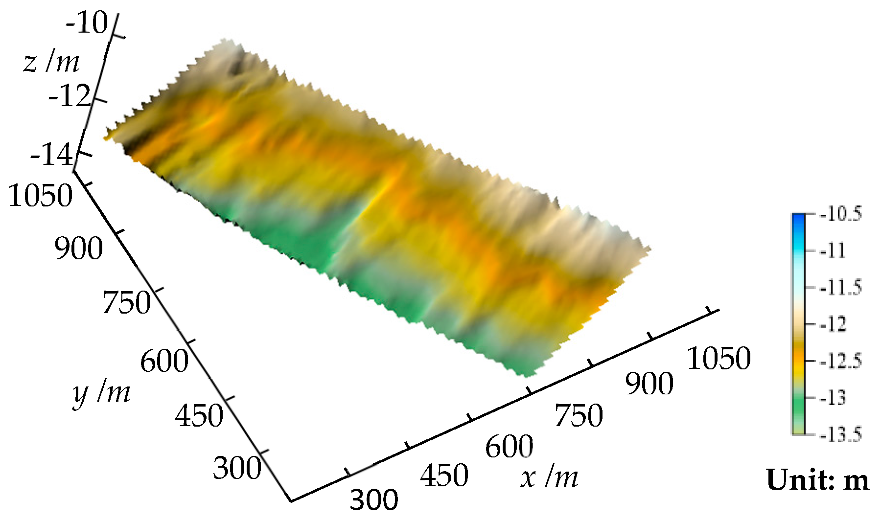
Figure 10.
The reconstructed terrain (a) and the real terrain constructed by SBS bathymetric data (b). ①–⑥ denote the topographic features in Strip I.
Figure 10.
The reconstructed terrain (a) and the real terrain constructed by SBS bathymetric data (b). ①–⑥ denote the topographic features in Strip I.

Figure 11.
Amplitude-frequency curves, high-frequency and low-frequency part differences of the reconstructed DEM and the bathymetric DEM. (a) Amplitude-Frequency curve of two DEMs; (b) the low-frequency part difference of the two DEMs; (c) the high-frequency part difference of the two DEMs.
Figure 11.
Amplitude-frequency curves, high-frequency and low-frequency part differences of the reconstructed DEM and the bathymetric DEM. (a) Amplitude-Frequency curve of two DEMs; (b) the low-frequency part difference of the two DEMs; (c) the high-frequency part difference of the two DEMs.

Figure 12.
(a) The reconstructed seabed topography and (b) the PDF curves of reconstruction biases at different across-track distances. The black lines denote the bathymetric lines; ①–⑥ denote the seabed features corresponding to those in Figure 6. 1–8 represent the bathymetric lines.
Figure 12.
(a) The reconstructed seabed topography and (b) the PDF curves of reconstruction biases at different across-track distances. The black lines denote the bathymetric lines; ①–⑥ denote the seabed features corresponding to those in Figure 6. 1–8 represent the bathymetric lines.
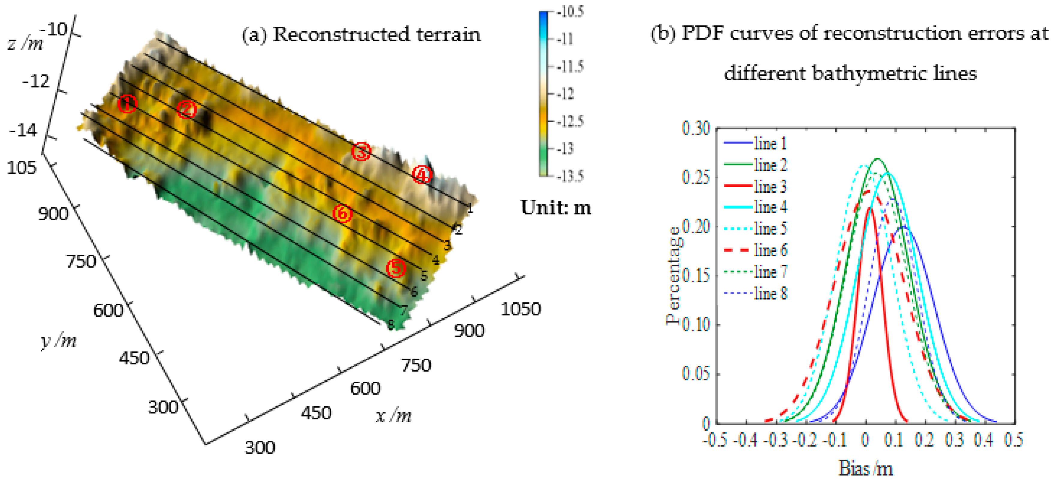
Figure 13.
Reconstructed seabed topography of the whole measurement area by the proposed method. ①–⑫ denote the seabed features as the same as those in Figure 5.
Figure 13.
Reconstructed seabed topography of the whole measurement area by the proposed method. ①–⑫ denote the seabed features as the same as those in Figure 5.

Figure 14.
PDF curves of biases of the reconstructed topographies in different areas. The PDF curves of the biases of the entire area (a), between strip I and II (b), between strip II and III (c).
Figure 14.
PDF curves of biases of the reconstructed topographies in different areas. The PDF curves of the biases of the entire area (a), between strip I and II (b), between strip II and III (c).

Figure 15.
Effects of sediment variations on the seabed reconstructions. (a) SSS image; (b) sediment classifications; (c) the actual bathymetric topography; (c1,c2) the reconstructed topographies by ignoring and considering the effects of seabed variations, respectively; (d1,d2) are PDF curves corresponding to (c1,c2).

Figure 16.
Bottom tracking under different situations. (a–c) show the normal situation and the situations of one-side water column and two-side ones covered by suspended solids. (b,c) are cited from [35].
Figure 16.
Bottom tracking under different situations. (a–c) show the normal situation and the situations of one-side water column and two-side ones covered by suspended solids. (b,c) are cited from [35].

Figure 17.
Convergence curves of the reconstruction model with (a) inappropriate and (b) appropriate initial terrains.
Figure 17.
Convergence curves of the reconstruction model with (a) inappropriate and (b) appropriate initial terrains.


Table 1.
Statistical parameters of seabed height biases.
| Max. (m) | Min. (m) | Mean (m) | STD (±m) |
|---|---|---|---|
| 0.28 | −0.36 | 0.00 | 0.13 |
Table 2.
Statistical parameters of the reconstruction biases of Strip I relative to the bathymetric data.
Table 2.
Statistical parameters of the reconstruction biases of Strip I relative to the bathymetric data.
| Max. | Min. | Mean | Standard Deviation |
|---|---|---|---|
| 0.30 | −0.43 | 0.00 | 0.12 |
Table 3.
Statistical parameters of the reconstruction biases at different bathymetric lines.
| Line | 1 | 2 | 3 | 4 | 5 | 6 | 7 | 8 | |
|---|---|---|---|---|---|---|---|---|---|
| Bias | |||||||||
| Max./m | 0.39 | 0.39 | 0.12 | 0.39 | 0.26 | 0.38 | 0.22 | 0.34 | |
| Min./m | −0.10 | −0.25 | −0.09 | −0.20 | −0.30 | −0.29 | −0.35 | −0.10 | |
| Mean/m | 0.12 | 0.04 | 0.01 | 0.07 | 0.00 | 0.01 | 0.03 | 0.10 | |
| Std/m | 0.10 | 0.10 | 0.04 | 0.10 | 0.09 | 0.11 | 0.10 | 0.08 | |
Table 4.
Statistical parameters of the biases of the reconstructed topographies in different areas.
| Biases (m) | Max. | Min. | Mean | Standard Deviation | |
|---|---|---|---|---|---|
| Area | |||||
| Entire measurement area | 0. 47 | −0.54 | 0.00 | 0.12 | |
| Overlapping area of Strip I & II | 0.44 | −0.54 | −0.08 | 0.14 | |
| Overlapping area of Strip II & III | 0.49 | −0.38 | 0.03 | 0.10 | |
© 2018 by the authors. Licensee MDPI, Basel, Switzerland. This article is an open access article distributed under the terms and conditions of the Creative Commons Attribution (CC BY) license (http://creativecommons.org/licenses/by/4.0/).
Share and Cite
MDPI and ACS Style
Zhao, J.; Shang, X.; Zhang, H. Reconstructing Seabed Topography from Side-Scan Sonar Images with Self-Constraint. Remote Sens. 2018, 10, 201. https://doi.org/10.3390/rs10020201
AMA Style
Zhao J, Shang X, Zhang H. Reconstructing Seabed Topography from Side-Scan Sonar Images with Self-Constraint. Remote Sensing. 2018; 10(2):201. https://doi.org/10.3390/rs10020201
Chicago/Turabian StyleZhao, Jianhu, Xiaodong Shang, and Hongmei Zhang. 2018. "Reconstructing Seabed Topography from Side-Scan Sonar Images with Self-Constraint" Remote Sensing 10, no. 2: 201. https://doi.org/10.3390/rs10020201
Note that from the first issue of 2016, this journal uses article numbers instead of page numbers. See further details here.