On the Applicability of Galileo FOC Satellites with Incorrect Highly Eccentric Orbits: An Evaluation of Instantaneous Medium-Range Positioning


Abstract
:1. Introduction
2. Analysis of Signal Power and Noise
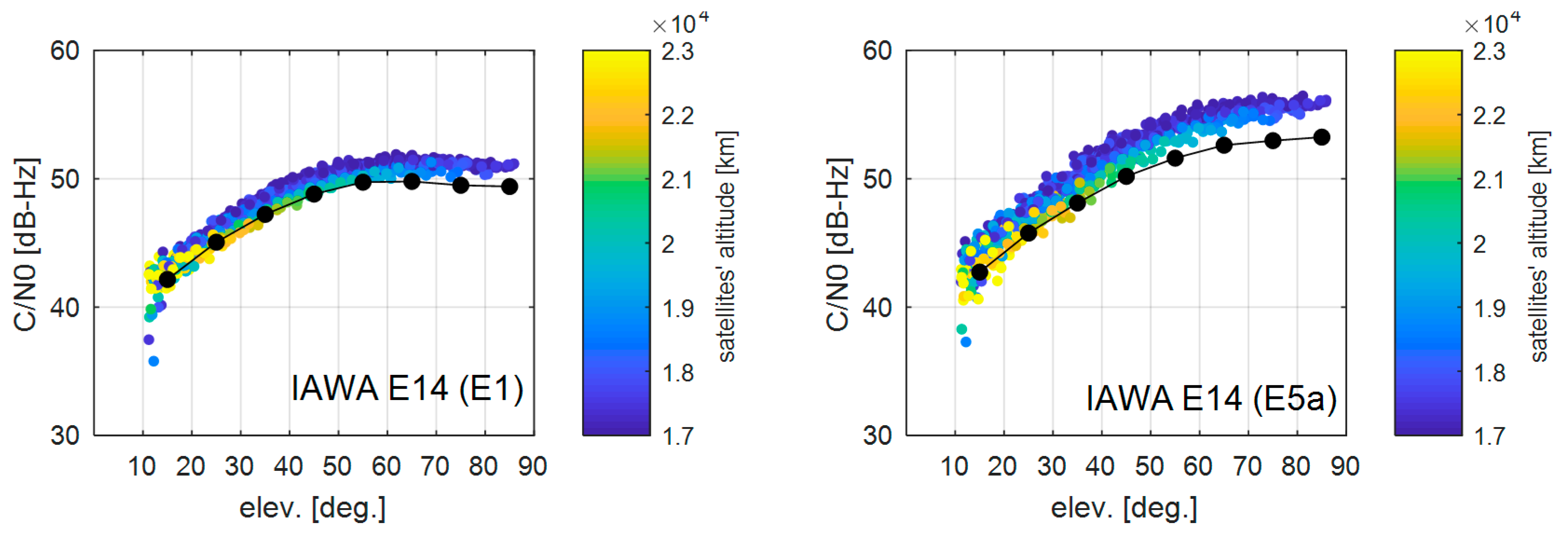
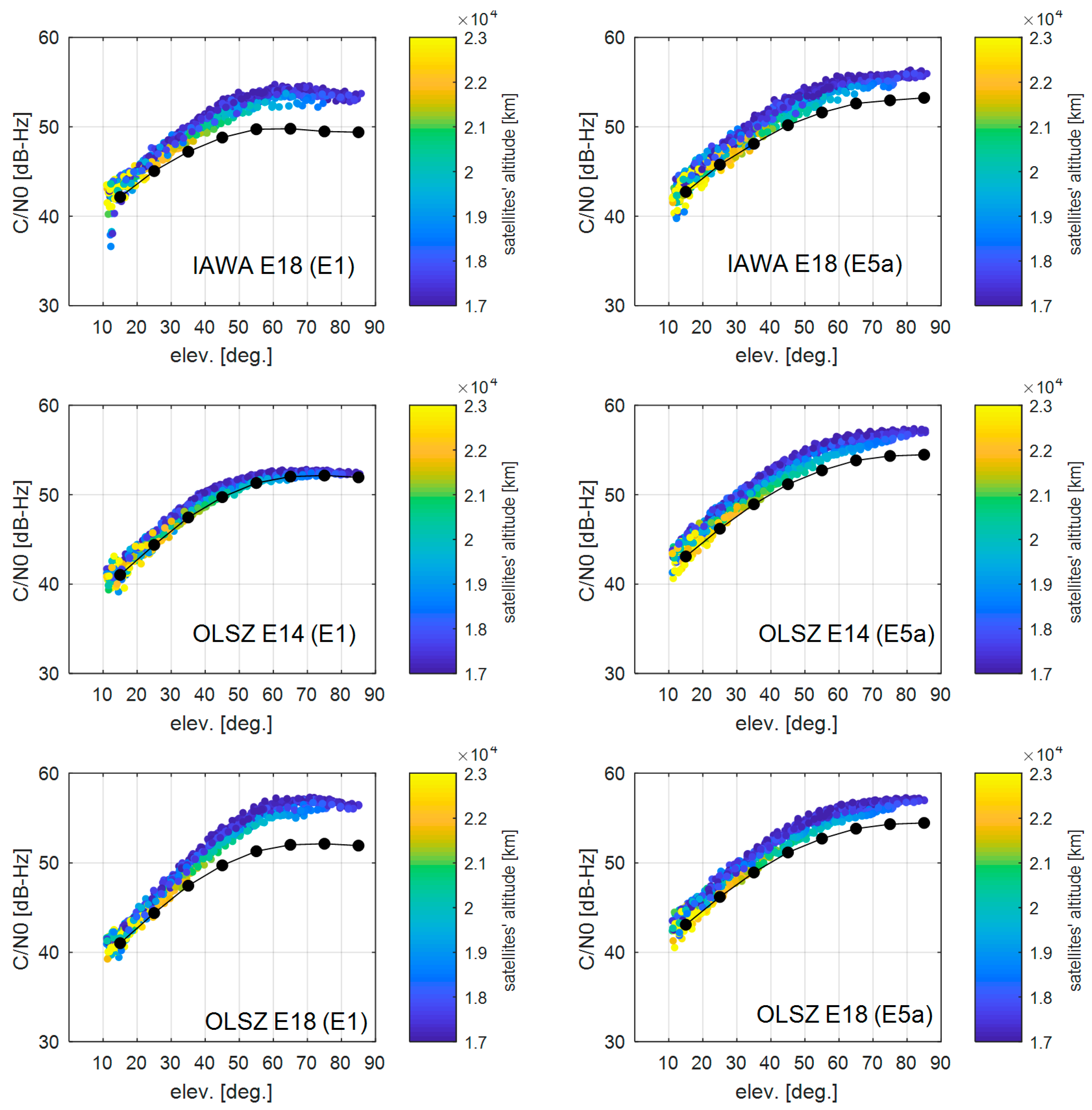
2.1. Signal Power
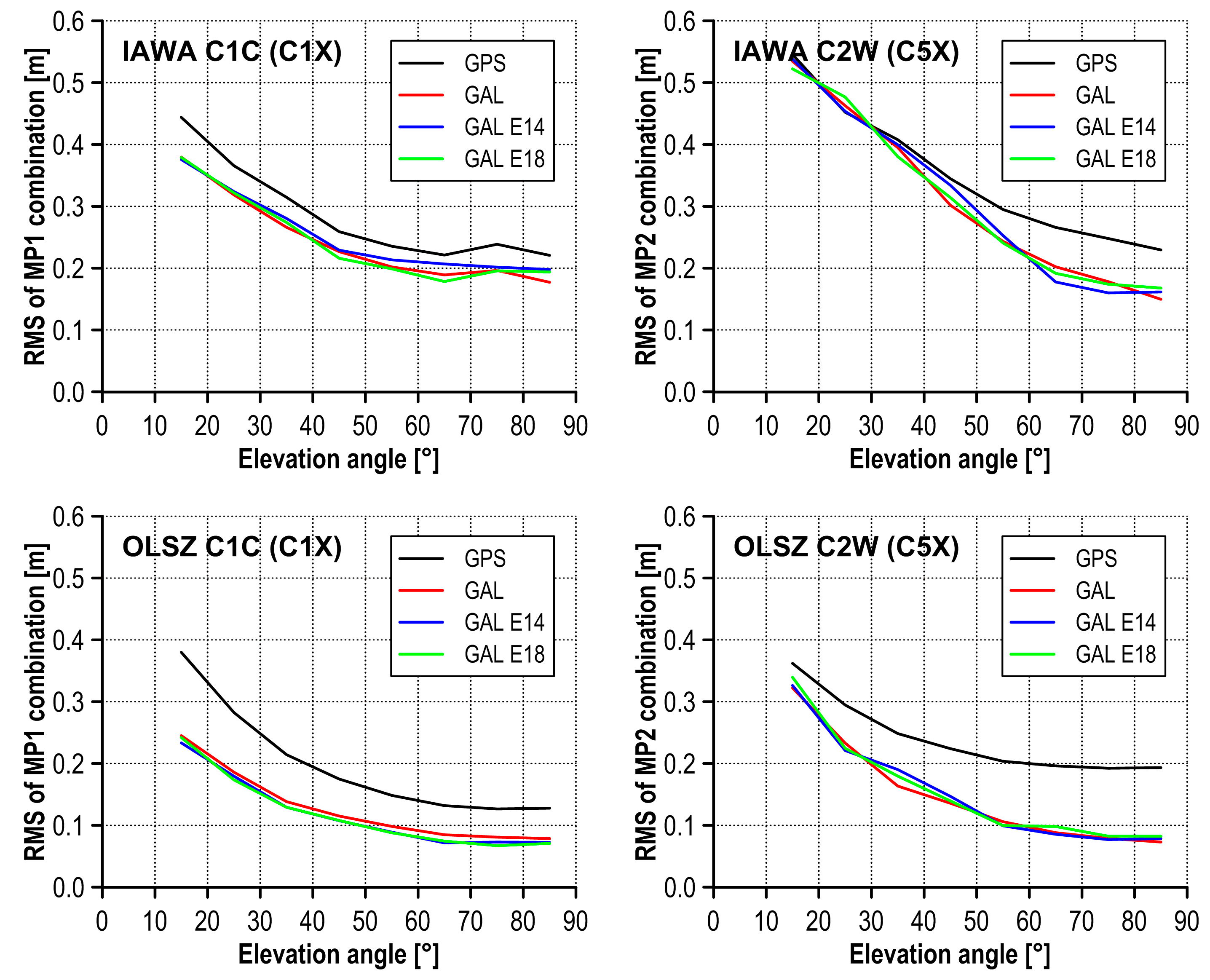
2.2. Code Measurement Noise
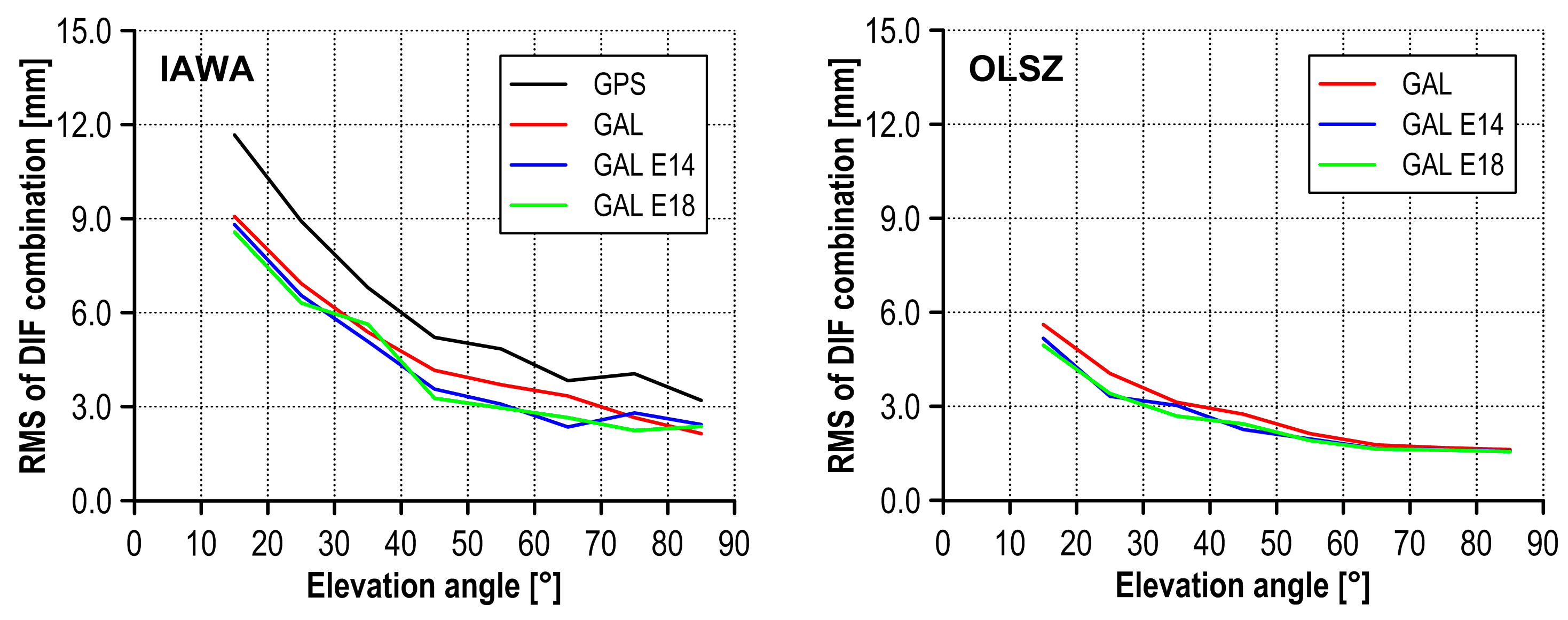
2.3. Phase Measurement Noise
3. Instantaneous Multi-Constellation Relative Positioning: Methodology and Performance
3.1. Loosely Combined Relative Positioning Model with Parameterised Ionospheric Delays
3.2. Performance Assessment of Precise Positioning with Focus on E14 and E18 Galileo Satellites
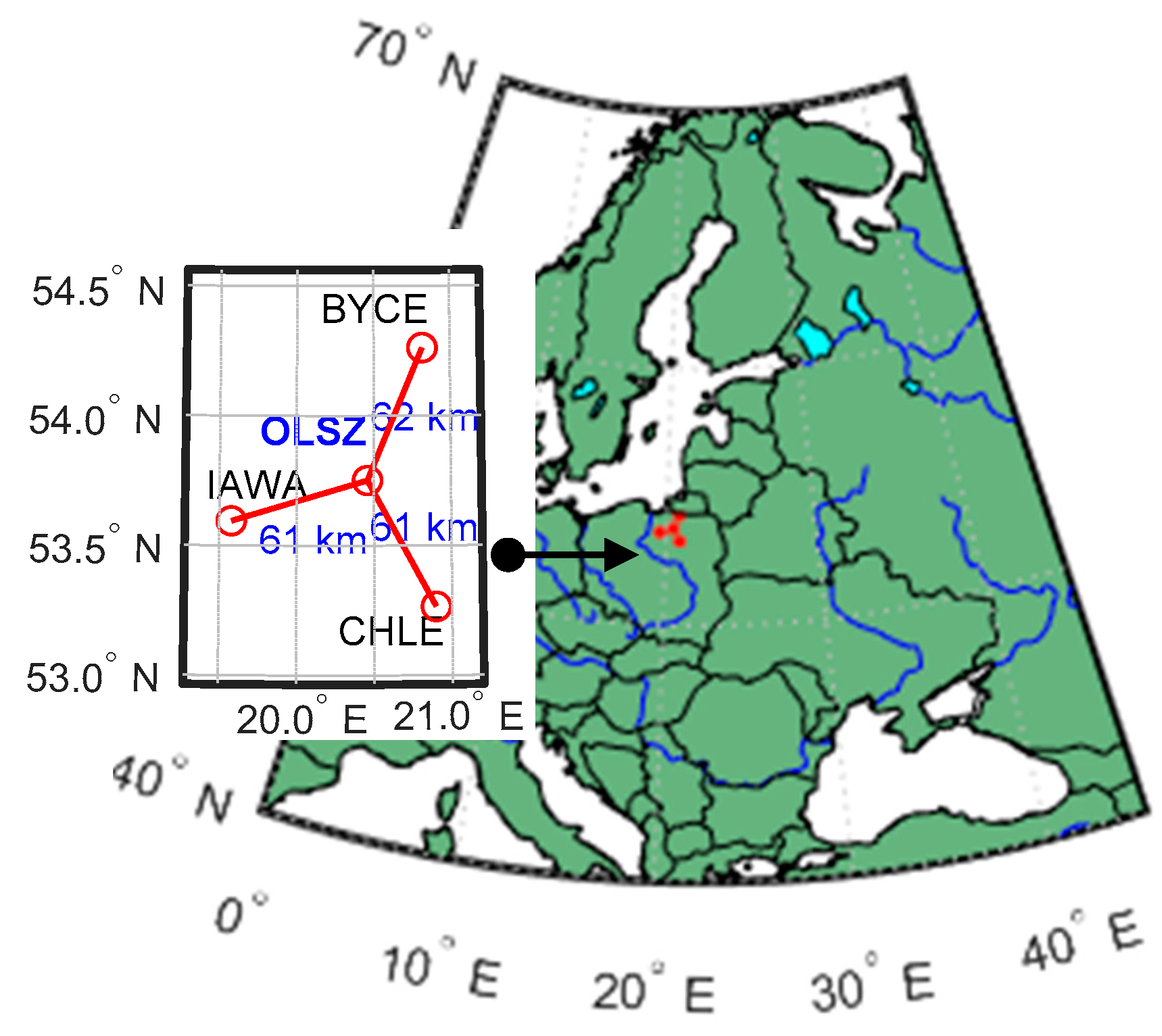
3.2.1. Data Selection & Experiment Design
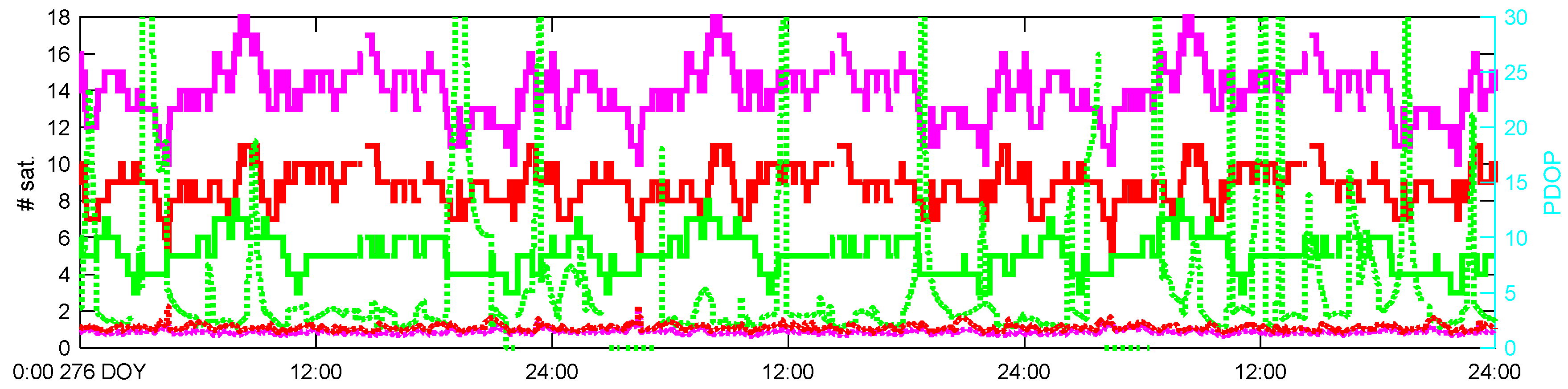
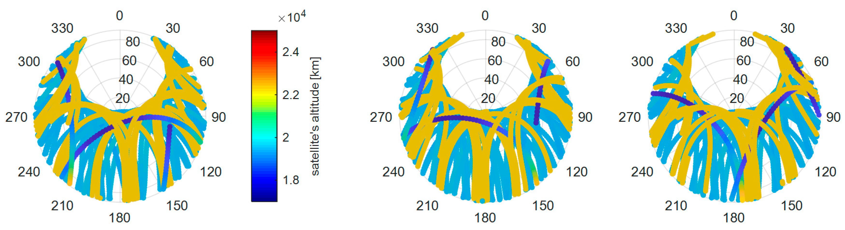
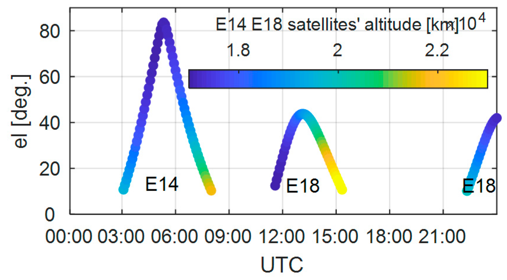
3.2.2. Geometry and Configuration of the Satellites during the Experiment
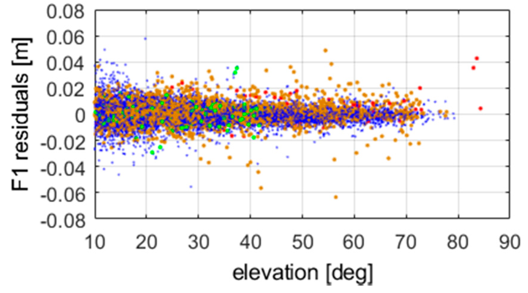
3.2.3. Performance Assessment of Instantaneous Positioning
4. Summary and Conclusions
Acknowledgments
Author Contributions
Conflicts of Interest
References
- Falcone, M.; Lugert, M.; Malik, M.; Crisci, M.; Rooney, E.; Jackson, C.; Threteway, M. GIOVE-A In Orbit Testing Results. In Proceedings of the 19th International Technical Meeting of the Satellite Division of The Institute of Navigation (ION GNSS 2006), Fort Worth, TX, USA, 26–29 September 2006; pp. 1535–1546. [Google Scholar]
- European Union. European GNSS (Galileo) Open Service Signal in Space Interface Control Document; Issue 1.2; OS SIS ICD; European Union: Brussels, Belgium, 2015. [Google Scholar]
- European Union. European GNSS (Galileo) Galileo Open Service Service Definition Document; Issue 1.0, OS SSD; European Union: Brussels, Belgium, 2016. [Google Scholar]
- Steigenberger, P.; Hauschild, A. First Galileo FOC Satellite on the Air—Will Be Employable for Surveying, Precise Positioning, and Geodesy. GPS World 2015, 26, 8–12. [Google Scholar]
- Sosnica, K.; Prange, L.; Kazmierski, K.; Bury, G.; Drozdzewski, M.; Zajdel, R.; Hadas, T. Validation of Galileo orbits using SLR with a focus on satellites launched into incorrect orbital planes. J. Geodesy 2017, 12, 1–18. [Google Scholar] [CrossRef]
- Ashby, N. Relativity in the global positioning system. Living Rev. Relat. 2003, 6, 1. [Google Scholar] [CrossRef] [PubMed]
- Delva, P.; Hees, A.; Bertone, S.; Richard, E.; Wolf, P. Test of the gravitational redshift with stable clocks in eccentric orbits: Application to Galileo satellites 5 and 6. Class. Quantum Gravity 2015, 32, 232003. [Google Scholar] [CrossRef]
- Delva, P.; Puchades, N. Testing the gravitational redshift with eccentric Galileo satellites. In Proceedings of the 6th International Colloquium Scientific and Fundamental Aspects of the GNSS/Galileo, Valencia, Spain, 25–27 October 2017; Technical University of Valencia: Valencia, Spain, 2017. [Google Scholar]
- Simsky, A.; Mertens, D.; Sleewaegen, J.M.; Hollreiser, M.; Crisci, M. Experimental results for the multipath performance of galileo signals transmitted by GIOVE—A satellite. Int. J. Navig. Obs. 2008, 2008, 13. [Google Scholar] [CrossRef]
- De Bakker, P.F.; van der Marel, H.; Tiberius, C.C.J.M. Geometry free undifferenced, single and double differenced analysis of single-frequency GPS, EGNOS, and GIOVE-A/B measurements. GPS Solut. 2009, 13, 305–314. [Google Scholar] [CrossRef]
- De Bakker, P.F.; Tiberius, C.C.J.M.; van der Marel, H.; van Bree, R.J.P. Short and zero baseline analysis of GPS L1 C/A, L5Q, GIOVE E1B, and E5aQ signals. GPS Solut. 2012, 16, 53–64. [Google Scholar] [CrossRef]
- Cai, C.; He, C.; Santerre, R.; Pan, L.; Cui, X.; Zhu, J. A comparative analysis of measurement noise and multipath for four constellations: GPS, BeiDou, GLONASS and Galileo. Surv. Rev. 2016, 48, 287–295. [Google Scholar] [CrossRef]
- Odijk, D.; Teunissen, P.J.G.; Khodabandeh, A. Galileo IOV RTK positioning: Standalone and combined with GPS. Surv. Rev. 2014, 46, 267–277. [Google Scholar] [CrossRef]
- Steigenberger, P.; Hugentobler, U.; Montenbruck, O. First demonstration of Galileo-only positioning. GPS World 2013, 24, 14–15. [Google Scholar]
- Cai, C.; Luo, X.; Liu, Z.; Xiao, Q. Galileo signal and positioning performance analysis based on four IOV satellites. Navigation 2014, 67, 810–824. [Google Scholar] [CrossRef]
- Gioia, C.; Borio, D.; Angrisano, A.; Gaglione, S.; Fortuny-Guasch, J. A Galileo IOV assessment: Measurement and position domain. GPS Solut. 2015, 19, 187–199. [Google Scholar] [CrossRef] [Green Version]
- Steigenberger, P.; Montenbruck, O. Galileo status: Orbits, clocks, and positioning. GPS Solut. 2017, 21, 319–331. [Google Scholar] [CrossRef]
- Pan, L.; Cai, C.; Santerre, R.; Zhang, X. Performance evaluation of single-frequency point positioning with GPS, GLONASS, BeiDou and Galileo. Surv. Rev. 2017, 70, 465–482. [Google Scholar] [CrossRef]
- Tegedor, J.; Øvstedal, O.; Vigen, E. Precise orbit determination and point positioning using GPS, Glonass, Galileo and BeiDou. J. Geod. Sci. 2014, 4, 65–73. [Google Scholar] [CrossRef]
- Afifi, A.; El-Rabbany, A. Single frequency GPS/Galileo precise point positioning using Un-differenced and between-satellite single difference measurements. Geomatica 2014, 68, 195–205. [Google Scholar] [CrossRef]
- Afifi, A.; El-Rabbany, A. An innovative dual frequency PPP model for combined GPS/Galileo observations. J. Appl. Geodesy 2015, 9, 27–34. [Google Scholar] [CrossRef]
- Cai, C.; Gao, Y.; Pan, L.; Zhu, J. Precise point positioning with quad-constellations: GPS, BeiDou, GLONASS and Galileo. Adv. Space Res. 2015, 56, 133–143. [Google Scholar] [CrossRef]
- Li, X.; Li, X.; Yuan, Y.; Zhang, K.; Zhang, X.; Wickert, J. Multi-GNSS phase delay estimation and PPP ambiguity resolution: GPS, BDS, GLONASS, Galileo. J. Geodesy 2017, 1–30. [Google Scholar] [CrossRef]
- Odijk, D.; Teunissen, P.J.G.; Huisman, L. First results of mixed GPS&GIOVE single-frequency RTK in Australia. J. Spat. Sci. 2012, 57, 3–18. [Google Scholar]
- Odolinski, R.; Teunissen, P.J.G.; Odijk, D. Combined BDS, Galileo, QZSS and GPS single-frequency RTK. GPS Solut. 2015, 19, 151–163. [Google Scholar] [CrossRef]
- Paziewski, J.; Wielgosz, P. Investigation of some selected strategies for multi-GNSS instantaneous RTK positioning. Adv. Space Res. 2017, 59, 12–23. [Google Scholar] [CrossRef]
- Zaminpardaz, S.; Teunissen, P.J.G. Analysis of Galileo IOV + FOC signals and E5 RTK performance. GPS Solut. 2017, 21, 1855–1870. [Google Scholar] [CrossRef]
- Hernandez-Pajares, M.; Juan, J.; Sanz, J.; Colombo, L. Feasibility of wide-area sub-decimeter navigation with GALILEO and modernized GPS. IEEE Trans. Geosci. Remote Sens. 2003, 41, 2128–2131. [Google Scholar] [CrossRef]
- Wielgosz, P.; Kashani, I.; Grejner-Brzezinska, D.A. Analysis of long-range network RTK during a severe ionospheric storm. J. Geodesy 2005, 79, 524–531. [Google Scholar] [CrossRef]
- Hernandez-Pajares, M.; Juan, J.M.; Sanz, J.; Aragon-Angel, A.; Ramos-Bosch, P.; Odijk, D.; Teunissen, P.J.G.; Samson, J.; Tossaint, M.; Albertazzi, M. Wide-Area RTK: High Precision Positioning on a Continental Scale. Inside GNSS 2010, 5, 35–46. [Google Scholar]
- Juan, J.M.; Sanz, J.; Hernández-Pajares, M.; Samson, J.; Tossaint, M.; Aragón-Àngel, A.; Salazar, D. Wide Area RTK: A satellite navigation system based on precise real-time ionospheric modelling Radio Science. Radio Sci. 2012, 47. [Google Scholar] [CrossRef]
- Paziewski, J.; Wielgosz, P. Assessment of GPS + Galileo and multi-frequency Galileo single-epoch precise positioning with network corrections. GPS Solut. 2014, 18, 571–579. [Google Scholar] [CrossRef]
- El-Mowafy, A.; Deo, M.; Rizos, C. On biases in Precise Point Positioning with multi-constellation and multi-frequency GNSS data. Meas. Sci. Technol. 2016, 27, 035102. [Google Scholar] [CrossRef]
- Choy, S.; Bisnath, S.; Rizos, C. Uncovering common misconceptions in GNSS Precise Point Positioning and its future prospect. GPS Solut. 2017, 21, 13–22. [Google Scholar] [CrossRef]
- Odijk, D.; Nadarajah, N.; Zaminpardaz, S. GPS, Galileo, QZSS and IRNSS differential ISBs: Estimation and application. GPS Solut. 2017, 21, 439–450. [Google Scholar] [CrossRef]
- Paziewski, J.; Wielgosz, P. Accounting for Galileo-GPS inter-system biases in precise satellite positioning. J. Geodesy 2015, 89, 81–93. [Google Scholar] [CrossRef]
- Paziewski, J.; Sieradzki, R.; Wielgosz, P. Selected properties of GPS and Galileo-IOV receiver Inter System Biases in multi GNSS data processing. Meas. Sci. Technol. 2015, 26, 095008. [Google Scholar] [CrossRef]
- Bock, Y.; Nikolaidis, R.; de Jonge, P.J.; Bevis, M. Instantaneous geodetic positioning at medium distances with the Global Positioning System. J. Geophys. Res. 2000, 105, 28233–28253. [Google Scholar] [CrossRef]
- Odijk, D. Instantaneous precise GPS positioning under geomagnetic storm conditions. GPS Solut. 2001, 5, 29–42. [Google Scholar] [CrossRef]
- Kashani, I.; Grejner-Brzezinska, D.A.; Wielgosz, P. Towards Instantaneous Network-Based RTK GPS Over 100 km Distance. Navigation 2005, 52, 239–245. [Google Scholar] [CrossRef]
- Genrich, J.F.; Bock, Y. Instantaneous geodetic positioning with 10–50 Hz GPS measurements: Noise characteristics and implications for monitoring networks. J. Geophys. Res. 2006, 111, B03403. [Google Scholar] [CrossRef]
- Próchniewicz, D.; Szpunar, R.; Brzeziński, A. Network-Based Stochastic Model for instantaneous GNSS real-time kinematic positioning. J. Surv. Eng. 2016, 142, 05016004. [Google Scholar] [CrossRef]
- Brunner, F.K.; Hartinger, H.; Troyer, L. GPS signal diffraction modelling: The stochastic SIGMAΔ model. J. Geodesy 1999, 73, 259–267. [Google Scholar] [CrossRef]
- Wieser, A.; Brunner, F.K. An Extended Weight Model for GPS Phase Observations. Earth Planets Space 2000, 52, 777–782. [Google Scholar] [CrossRef]
- Montenbruck, O.; Hauschild, A.; Steigenberger, P.; Hugentobler, U.; Teunissen, P.; Nakamura, S. Initial assessment of the COMPASS/BeiDou-2 regional navigation satellite system. GPS Solut. 2013, 17, 211–222. [Google Scholar] [CrossRef]
- Hauschild, A.; Montenbruck, O.; Sleewaegen, J.M.; Huisman, L.; Teunissen, P.J.G. Characterization of Compass M-1 signals. GPS Solut. 2012, 16, 117–126. [Google Scholar] [CrossRef]
- Estey, L.H.; Meertens, C.M. TEQC: The multi-purpose toolkit for GPS/GLONASS data. GPS Solut. 1999, 3, 42–49. [Google Scholar] [CrossRef]
- Montenbruck, O.; Hugentobler, U.; Dach, R.; Steigenberger, P.; Hauschild, A. Apparent clock variations of the Block IIF-1 (SVN62) GPS satellite. GPS Solut. 2011, 16, 303–313. [Google Scholar] [CrossRef]
- Julien, O.; Cannon, M.E.; Alves, P.; Lachapelle, G. Triple frequency ambiguity resolution using GPS/Galileo. Eur. J. Navig. 2004, 2, 51–56. [Google Scholar]
- Gao, W.; Gao, C.; Pan, S.; Meng, X.; Xia, Y. Inter-System Differencing between GPS and BDS for Medium-Baseline RTK Positioning. Remote Sens. 2017, 9, 948. [Google Scholar] [CrossRef]
- Bock, Y.; Gourevitch, S.A.; Counselman, C.C.; King, R.W.; Abbot, R.I. Interferometric analysis of GPS phase observations. Manuscr. Geodaet. 1986, 11, 282–288. [Google Scholar]
- Teunissen, P.J.G. The geometry-free GPS ambiguity search space with a weighted ionosphere. J. Geodesy 1997, 71, 370–383. [Google Scholar] [CrossRef]
- Wielgosz, P. Quality assessment of GPS rapid static positioning with weighted ionospheric parameters in generalized least squares. GPS Solut. 2011, 15, 89–99. [Google Scholar] [CrossRef]
- Paziewski, J. Study on desirable ionospheric corrections accuracy for network-RTK positioning and its impact on time-to-fix and probability of successful single-epoch ambiguity resolution. Adv. Space Res. 2016, 57, 1098–1111. [Google Scholar] [CrossRef]
- Paziewski, J. Precise GNSS single epoch positioning with multiple receiver configuration for medium-length baselines: Methodology and performance analysis. Meas. Sci. Technol. 2015, 26, 035002. [Google Scholar] [CrossRef]
- Odijk, D. Weighting Ionospheric Corrections to Improve Fast GPS Positioning Over Medium Distances. In Proceedings of the 13th International Technical Meeting of the Satellite Division of the Institute of Navigation (ION GPS 2000), Salt Lake City, UT, USA, 19–22 September 2000. [Google Scholar]
- Prange, L.; Orliac, E.; Dach, R.; Arnold, D.; Beutler, G.; Schaer, S.; Jäggi, A. CODE’s five-system orbit and clock solution—The challenges of multi-GNSS data analysis. J. Geodesy 2017, 91, 345–360. [Google Scholar] [CrossRef]
- Chang, X.W.; Yang, X.; Zhou, T. MLAMBDA: A modified LAMBDA method for integer least-squares estimation. J. Geodesy 2005, 79, 552–565. [Google Scholar] [CrossRef]
- Wang, J.; Stewart, M.; Tsakiri, M. A discrimination test procedure for ambiguity resolution on-the-fly. J. Geodesy 1998, 72, 644–653. [Google Scholar] [CrossRef]
- Available online: http://vrsnet.pl (accessed on 20 October 2017).
- He, H.; Li, J.; Yang, Y.; Xu, J.; Guo, H.; Wang, A. Performance assessment of single- and dual-frequency Beidou/GPS single-epoch kinematic positioning. GPS Solut. 2014, 18, 393–403. [Google Scholar] [CrossRef]
- Deng, C.; Tang, W.; Liu, J.; Shi, C. Reliable single-epoch ambiguity resolution for short baselines using combined GPS/Beidou system. GPS Solut. 2014, 18, 375–386. [Google Scholar] [CrossRef]
- Paziewski, J.; Sieradzki, R. Integrated GPS+BDS instantaneous medium baseline RTK positioning: Signal analysis, methodology and performance assessment. Adv. Space Res. 2017, 60, 2561–2573. [Google Scholar] [CrossRef]
- Han, S. Quality-control issues relating to instantaneous ambiguity resolution for real-time GPS kinematic positioning. J. Geodesy 1997, 71, 351–361. [Google Scholar] [CrossRef]


| Nominal Orbit | GSAT0201 (5-Doresa) | GSAT0202 (6-Milena) | |
|---|---|---|---|
| PRN Number/NORAD ID | E18/40128 | E14/40129 | |
| Launch Date | 22 August 2014 | 22 August 2014 | |
| Signal Transmission Date | 29 November 2014 | 17 March 2015 | |
| Semi-major axis (km) | 29,599.8 | 27,978 | 27,978 |
| Eccentricity | 0.0001 | 0.15601 | 0.15167 |
| Revolution period (h) | 14.08 | 12.97 | 12.97 |
| Inclination (°) | 56 | 49.775 | 49.874 |
| Minimum orbital height (km) | 23,220 | 17,382 | 17,382 |
| Maximum orbital height (km) | 23,240 | 25,818 | 25,818 |
| Station | GPS | Galileo (Except #14 and E18) | Galileo E14 | Galileo E18 | ||||
|---|---|---|---|---|---|---|---|---|
| MP1 | MP2 | MP1 | MP2 | MP1 | MP2 | MP1 | MP2 | |
| BYCE | 0.20 | 0.21 | 0.16 | 0.14 | 0.16 | 0.13 | 0.16 | 0.13 |
| CHLE | 0.21 | 0.22 | 0.19 | 0.13 | 0.17 | 0.13 | 0.18 | 0.13 |
| IAWA | 0.22 | 0.23 | 0.18 | 0.15 | 0.20 | 0.16 | 0.19 | 0.17 |
| OLSZ | 0.13 | 0.19 | 0.08 | 0.07 | 0.07 | 0.08 | 0.07 | 0.08 |
| Date and Time of Session | 3–5 October 2017 00:00–24:00 UTC |
|---|---|
| Baselines’ lengths | 61–62 km |
| GNSS constellations | GPS & Galileo |
| Observation types | dual frequency phase and pseudorange |
| Frequencies | L1 & L2 (GPS), E1 & E5a (Galileo) |
| Session length & solution | Instantaneous (single-epoch) relative solution |
| # of solutions per day | 288 independent single-epoch solution per day (@300 s) |
| Tropospheric delay mitigation | a priori values from Modified Hopfield + GMF mapping function + tightly constrained estimation of the residual ZTD |
| Ionospheric delay mitigation | constrained estimation of DD first-order ionospheric delays (ionosphere float model) |
| Elevation cut-off angle | 10° |
| Ephemeris | Precise final from CODE (COM) [57] |
| Observation weighting scheme | Elevation-dependent |
| Ambiguities handling | Fixed to integers with M-Lambda [58] and validated with W-ratio [59] |
| A priori standard deviation of undifferenced observations | 0.2 m and 0.002 m for code and phase (E1/L1), respectively |
| Estimation method | least squares adjustment with a priori parameter constraining (single-epoch) |
| # | Constellations |
|---|---|
| 1. | GPS |
| 2. | Galileo |
| 3. | Combined GPS + Galileo with E14 and E18 |
| 4. | Combined GPS + Galileo without E14 and E18 |
| GPS | Galileo | GPS + Galileo with E14 & E18 | GPS + Galileo without E14 & E18 Satellites | |
|---|---|---|---|---|
| 3 October 2017 (276 DOY) | ||||
| N | 0.9 | 1.5 | 1.2 | 1.1 |
| E | 0.6 | 1.2 | 0.8 | 0.8 |
| U | 2.1 | 5.5 | 2.9 | 2.3 |
| 4 October 2017 (277 DOY) | ||||
| N | 0.9 | 1.7 | 1.2 | 1.1 |
| E | 0.6 | 1.4 | 0.8 | 0.8 |
| U | 2.0 | 6.6 | 2.5 | 2.5 |
| 5 October 2017 (278 DOY) | ||||
| N | 1.2 | 1.9 | 1.3 | 1.3 |
| E | 0.6 | 1.3 | 0.9 | 0.9 |
| U | 2.8 | 12.8 | 3.3 | 3.4 |
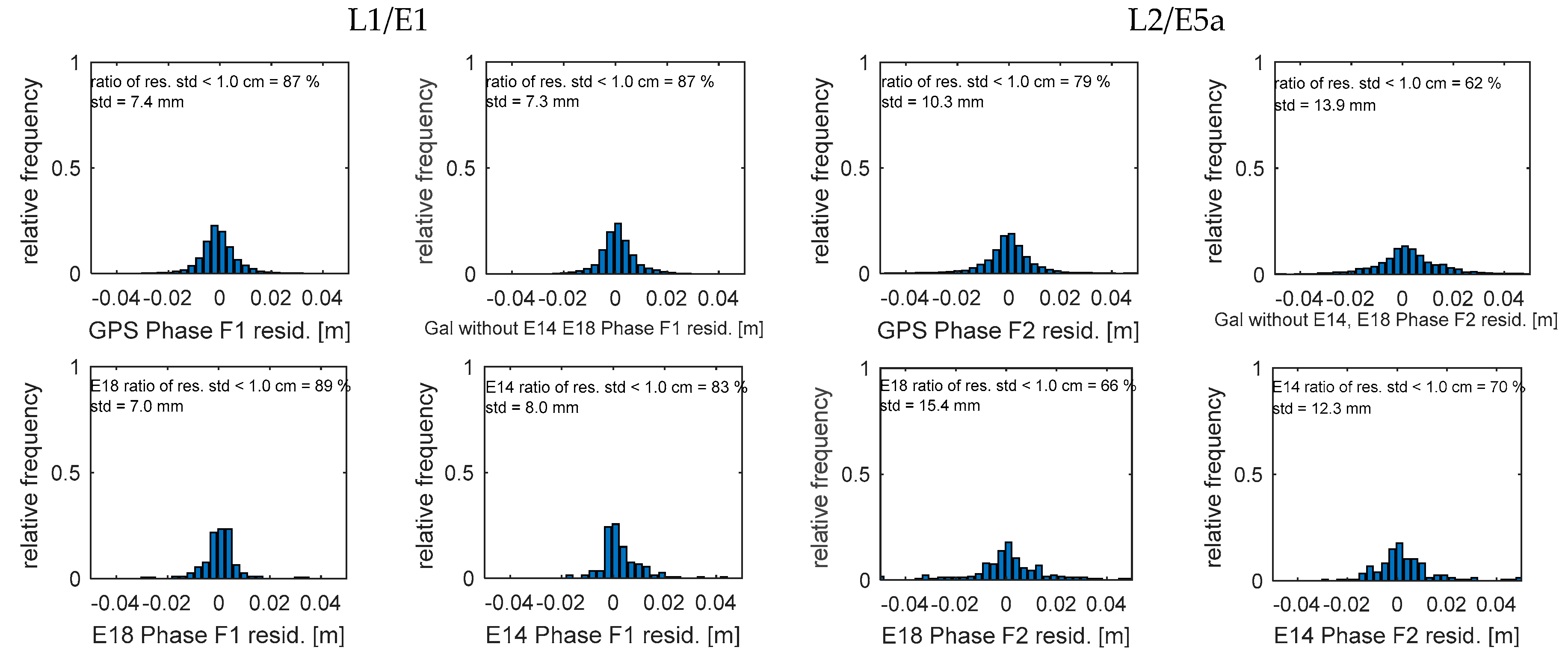
| GPS L1 | GPS L2 | Gal E1 | E14 E1 | E18 E1 | Gal E5a | E14 E5a | E18 E5a | |
|---|---|---|---|---|---|---|---|---|
| 3 October | 7.4 | 10.3 | 7.3 | 8.0 | 7.0 | 13.9 | 12.3 | 15.4 |
| 4 October | 7.0 | 10.3 | 7.3 | 8.7 | 7.5 | 14.6 | 16.3 | 15.8 |
| 5 October | 7.8 | 10.3 | 7.7 | 8.5 | 6.5 | 14.6 | 17.3 | 14.7 |
© 2018 by the authors. Licensee MDPI, Basel, Switzerland. This article is an open access article distributed under the terms and conditions of the Creative Commons Attribution (CC BY) license (http://creativecommons.org/licenses/by/4.0/).
Share and Cite
Paziewski, J.; Sieradzki, R.; Wielgosz, P. On the Applicability of Galileo FOC Satellites with Incorrect Highly Eccentric Orbits: An Evaluation of Instantaneous Medium-Range Positioning. Remote Sens. 2018, 10, 208. https://doi.org/10.3390/rs10020208
Paziewski J, Sieradzki R, Wielgosz P. On the Applicability of Galileo FOC Satellites with Incorrect Highly Eccentric Orbits: An Evaluation of Instantaneous Medium-Range Positioning. Remote Sensing. 2018; 10(2):208. https://doi.org/10.3390/rs10020208
Chicago/Turabian StylePaziewski, Jacek, Rafal Sieradzki, and Pawel Wielgosz. 2018. "On the Applicability of Galileo FOC Satellites with Incorrect Highly Eccentric Orbits: An Evaluation of Instantaneous Medium-Range Positioning" Remote Sensing 10, no. 2: 208. https://doi.org/10.3390/rs10020208