The Accuracies of Himawari-8 and MTSAT-2 Sea-Surface Temperatures in the Tropical Western Pacific Ocean

1
Meteorology and Ocean Sciences & Coastal Studies, College of Science and Technology, Millersville University, Millersville, PA 17551, USA
2
Ocean Sciences, Rosenstiel School of Marine and Atmospheric Science, University of Miami, Miami, FL 33149, USA
*
Author to whom correspondence should be addressed.
†
Current affiliation: Center for Remote Sensing, College of Earth, Ocean, and Environment, University of Delaware, Newark, DE 19716, USA.
Remote Sens. 2018, 10(2), 212; https://doi.org/10.3390/rs10020212
Submission received: 20 November 2017
/
Revised: 16 January 2018
/
Accepted: 24 January 2018
/
Published: 1 February 2018
(This article belongs to the Special Issue Sea Surface Temperature Retrievals from Remote Sensing)
Abstract
:Over several decades, improving the accuracy of Sea-Surface Temperatures (SSTs) derived from satellites has been a subject of intense research, and continues to be so. Knowledge of the accuracy of the SSTs is critical for weather and climate predictions, and many research and operational applications. In 2015, the operational Japanese MTSAT-2 geostationary satellite was replaced by the Himawari-8, which has a visible and infrared imager with higher spatial and temporal resolutions than its predecessor. In this study, data from both satellites during a three-month overlap period were compared with subsurface in situ temperature measurements from the Tropical Atmosphere Ocean (TAO) array and self-recording thermometers at the depths of corals of the Great Barrier Reef. Results show that in general the Himawari-8 provides more accurate SST measurements compared to those from MTSAT-2. At various locations, where in situ measurements were taken, the mean Himawari-8 SST error shows an improvement of ~0.15 K. Sources of the differences between the satellite-derived SST and the in situ temperatures were related to wind speed and diurnal heating.

1. Introduction
Sea-surface temperature (SST) is a key variable for the study of the climate, weather, and ocean. The tropical western Pacific Ocean and eastern Indian Ocean, often referred to as the Tropical Warm Pool (TWP), have some of the highest SSTs (e.g., [1]). High SSTs throughout the tropical belt lead to meridional convergence in the lower troposphere and convection producing the clouds of the intertropical convergence zone (ITCZ) [2] which, being the ascending arm of the Hadley Cells to the north and south, is a driver of the large scale atmospheric circulation. As such, it is also a major part of the earth’s hydrological cycle [3]. The bright cloud tops in the ITCZ also influence the regional planetary albedo and thus influence the radiative heat budget of the earth. The vertical atmospheric motion is driven by the high SSTs in the equatorial regions [4]. The SST is also an indicator of the upper ocean heat content that is closely connected to the generation and intensification of cyclones in the TWP [5,6]. The cyclones frequently make landfall to the west, where damage and loss of life can be extreme (e.g., [7]). Improved accuracy of SSTs is critical for better forecasts of such events.
A further aspect of high temperatures in the tropics is the risk to coral reefs, which are damaged by elevated temperatures both when occurring episodically, such as on diurnal time scales [8,9] and over several days [10,11]. Dire consequences follow when elevated temperatures are sustained over weeks and months [12]. If the temperatures revert to the range to which they are acclimated, the corals can recover, however extended periods of high temperatures can lead to extensive coral mortality [9,13]. The defense mechanism of corals when subjected to elevated temperatures is to expel the symbiotic algae (zooxanthellae) living in their tissues causing the coral to lose their color, an effect widely referred to as coral bleaching. Coral bleaching can also result from anomalously low temperatures [14], especially where the corals are exposed to cold air temperatures at low tide [15]. The corals are also stressed by increasing ocean acidification [16,17].
The western Pacific and eastern Indian Oceans are home to extensive coral reefs, including those in the so-called Coral Triangle that encompasses the waters between the island of Borneo in the west and the Solomon Islands in the east, and the northern extent of the Philippines in the north, and the Timor, Arafura, and Coral Seas to the south [18]. The Coral Triangle contains the highest diversity of corals and of the species that are associated with them, including reef fishes [19]. The Coral Triangle does not exist in isolation, but is embedded in a much larger area of corals and high marine biodiversity that includes the Great Barrier Reef (GBR) off Queensland, Australia, to the south. At present, the GBR is experiencing extensive and severe bleaching, especially in the northern part where mortality is very high (>50%); the GBR coral bleaching is the worst on record [20,21]. The episode began in 2014 with record high SSTs through much of the Coral Triangle and GBR, and is part of a global event that is especially severe in the Pacific and Indian Oceans [22]. The intensity and spatial extent of this, and past severe bleaching occurrences, are clearly linked to the spatial patterns of elevated SSTs [12], and are expected to become worse as the oceans warm [12,23]. Thus, the areas of the Coral Triangle and GBR present a very pressing need for accurate measurements of ocean temperature over long periods and over large areas.
A valuable source of global near-surface ocean temperatures are those measured from surface drifting buoys [24] deployed to provide measurements for weather forecasting and studying surface currents. The temperature measurements, taken at a depth of about 20 cm in calm seas, are in widespread use [25,26], but equatorial upwelling and surface current divergence tends to remove the drifters from the tropics [27,28]. Thus, there is a paucity of measurements in the Coral Triangle and GBR regions.
Near-surface temperatures are measured in the tropics by thermometers of the Global Tropical Moored Buoy Array, which, in the Tropical Western Pacific Ocean, comprises the Triangle Trans-Ocean Buoy Network (TRITON; [29]). This is a deep-water mooring array, and so does not extend into the shallow waters where the corals are found. In contrast, temperature measurements have been made by the Australian Institute of Marine Science (AIMS) for many years by self-recording thermometers deployed at the coral depths by divers. These measurements are very good indicators of the thermal stress experienced by the corals and, being recorded during our analysis period with a 10-min resolution, provide data that resolve rapid changes, such as those associated with diurnal heating [30]. However, they are relatively sparse in space, and the data loggers have to be recovered before the temperatures can be analyzed.
Thus, the surface temperature fields derived from satellites are a very attractive source of information to study the potential threats to the wellbeing of the corals, especially as a recent study has shown they are an accurate proxy for temperatures at the depths of the corals [31], even though the satellite-derived temperatures are skin temperatures (SSTskin; [32,33]). Satellite derived SSTs cover large areas and those from geostationary satellites positioned over the Equator of the Pacific Ocean provide frequent measurements over the Coral Triangle and GBR. However, the appropriate application of satellite-derived SSTs to assessing the thermal conditions experienced by corals depends on knowledge of the errors and uncertainties in the SSTs retrieved from the satellite measurements. Our objective is to determine the accuracies of SSTs derived from geostationary satellites in the Tropical Western Pacific Ocean, including the Coral Triangle and the GBR. Our focus will be on SSTs derived from infrared radiometers on geostationary satellites, as these provide more rapid sampling than the polar orbiters which offers the possibility of capturing short period heating events [31]. Given that clouds obscure the surface in the infrared and thus prevent the derivation of SSTs, the rapid sampling by geostationary sensors increases the likelihood of determining SSTs at given locations as clouds pass. The accuracies of the satellite-derived SSTs will be established by comparisons with in situ measurements from the Triangle Trans-Ocean buoy Network (TRITON) moored buoys in the western part of the TAO array and from the GBR temperature loggers.
The paper is organized as follows: the next section introduces the data, beginning with the satellite retrieved SSTs and analysis methods, followed by a presentation of the results. A discussion of the results comes before the conclusions, which includes suggestions for further work.
2. Materials and Methods
Himawari-8, the first of a new generation of geostationary meteorology satellites of the Japan Meteorological Agency (JMA), began their operation on 7 July 2015. Himawari-8 replaced the MTSAT-2 (Multifunctional Transport Satellite-2, also referred to as Himawari-7). Though Himawari-8 became operational in July, MTSAT-2 continued operation until 4 December 2015 [34]. Himawari-8 is located at 140.7°E above the equator while the MTSAT-2 is located at 145°E above the equator. Himawari-8 carries the Advanced Himawari Imager (AHI), which has significant improvements in comparison to the imager onboard MTSAT-2. The AHI is capable of generating full disk images with a 10-min sampling frequency. The AHI has 16 spectral bands of which four are infrared (IR), λ = 8.60, 10.45, 11.20, and 12.35 μm [35,36], that are used for SST retrievals. These IR bands have a spatial resolution of 2 km at nadir. The temporal and spatial resolutions of Himawari-8 AHI are improved from those of the MTSAT-2 imager, which has only five spectral bands. Three of the five spectral bands used for IR SST retrievals include λ = 3.75, 10.8, and 12.0 μm [37] which have a 4 km spatial resolution and sampling intervals of 60 min [38,39]. Table 1 summarizes the satellite characteristics. SST fields from both satellites are provided by the National Oceanic and Atmospheric Administration (NOAA) in GHRSST Level-2 Pre-processed format (L2P; [32]). A recent study by Kramar et al. [40] found that Himawari-8 AHI SSTs derived using NOAA’s Advanced Clear-sky Processor for Oceans (ACSPO; [41]) show better accuracy than those produced by the Japan Aerospace Exploration Agency (JAXA). Based on this result, the MTSAT-2 and Himawari-8 SSTs used here are those produced by the NOAA Office of Satellite Products and Operations (OSPO).
The MTSAT-2 SSTs were derived using the long-established Non-Linear SST atmospheric correction algorithm [37] that uses measurements taken in the thermal infrared centered at λ = 10.8 and 12.0 μm:
where Tn are brightness temperatures, in K, measured at n = rounded integer values of λ, θ is the satellite zenith angle and Tsfc is a prior estimate of the surface temperature. Equation (1) can be used during both day and night. The coefficients are derived from a correlation analysis between the satellite brightness temperature measurements and coincident subsurface temperatures from buoys. The night-time algorithm, also due to Walton, Pichel, Sapper, and May [37], includes measurements from a third channel centered at λ = 3.75 μm:
SST = a0 + a1 × T11 + a2 × (T11 − T12) × Tsfc + a3 × (T11 − T12) × (sec(θ) − 1)
SST = a0 + a1 × T11 + a2 × (T3.7 − T12) × Tsfc + a3 × (sec(θ) − 1)
The measurements in the mid-infrared atmospheric transmission window, T3.7, suffer from contamination from scattered and reflected solar radiation that occurs during the day, so these measurements can only be used at night. The metadata in the MTSAT-2 files indicate that the retrieved SSTs are a skin temperature.
The ACSPO SST atmospheric correction algorithm applied to Himawari-8 AHI uses measurements from four infrared bands, labeled 11, 13, 14, and 15 at central wavelengths, λ = 8.60, 10.45, 11.20, and 12.35 μm [35,36]; it takes the form [40]:
where here Tsfc is an estimate of the surface temperature taken from the daily Canadian Meteorological Center (CMC) L4 SST analysis [42]. The coefficients ai are derived from regression analysis of collocated, contemporaneous brightness temperature measurements of the satellite radiometer with those of quality-controlled subsurface temperatures measured from drifting and moored buoys in the iQuam data set (in situ SST Quality Monitor; [43]). Thus the Himawari-8 AHI SSTs are considered a “subskin” temperature [40]. Since Equation (3) does not use brightness temperature measurements in the mid-infrared atmospheric transmission window it can be used for both daytime and night-time SST retrievals. For successful retrieval of SST, the brightness temperatures have to be screened to remove all measurements that include a component of emission from clouds. The Himawari-8 AHI data were taken from ftp://ftp.star.nesdis.noaa.gov/pub/sod/sst/acspo_data/l2/ahi/.
SST = a0 + a1 × T10 + a2 × (T10 − T12) + a3 × (T10 − T9) × sec(θ) + a4 × (T10 − T11) × sec(θ)
+ a5 × (T10 − T9) × Tsfc + a6 × (T10 − T11) × Tsfc + a7 × (T10 − T12) × Tsfc
+ a5 × (T10 − T9) × Tsfc + a6 × (T10 − T11) × Tsfc + a7 × (T10 − T12) × Tsfc
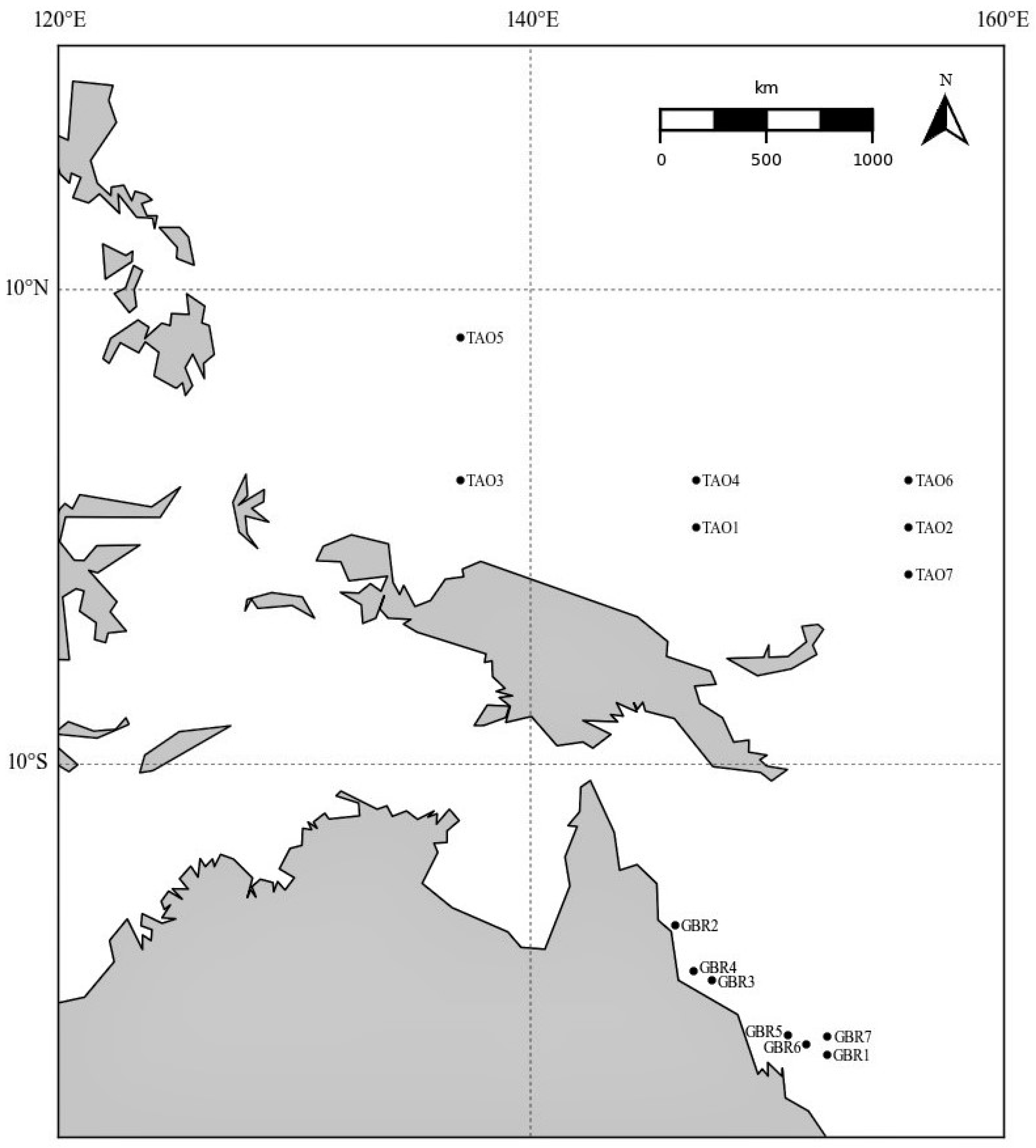
In this study, satellite SSTs were compared to multiple subsurface in situ temperature measurements. These in situ stations include seven TRITON moored buoys from the TAO array and seven self-recording thermometers attached to corals in the GBR (Table 2). The accuracy of the near-surface thermometers on the TRITON buoys is 0.05 K [44], and that of the GBR thermometers is better than ±0.1 K [11].
The TAO data used here were provided by NOAA/PMEL (Pacific Marine Environmental Laboratory (https://www.pmel.noaa.gov/tao/drupal/disdel/) and in situ data from the GBR were provided by the Australian Institute of Marine Science (AIMS). SSTs derived from Himawari-8 are subskin SSTs, whereas the in situ measurements are at 1.5 m depth on the TRITON buoys of the TAO array (http://www.jamstec.go.jp/jamstec/TRITON/real_time/overview/po-t1), the depths of the thermometers on the GBR vary. The depths of the GBR thermometers are given below the lowest astronomical tide and thus the depths below the surface will depend on the state of the tide; typically the tidal amplitudes are 5 m for spring tides and 2 m for neap tides [45]. Three months (1 August 2015–31 October 2015) of data were compiled during a period when both satellites were operational. The selection of in situ stations (Table 2, Figure 1) required data to be available in this period. A 5 × 5 pixel box of data was extracted from both satellites’ images around each in situ location. This was to ensure there would an adequate amount of satellite data of the best quality (quality flag 5). The best quality data were spatially averaged to give one satellite measurement for each in situ location for each comparison.
Himawari-8 AHI and the thermometers in the GBR had a temporal resolution of 10 min, but the measurements were not synchronized. Data from the GBR were linearly interpolated to match the times of the Himawari-8 data. MTSAT-2 and the TAO array had an hourly temporal resolution; data from the GBR and Himawari-8 were averaged to match this hourly temporal resolution; the averaging process is summarized in Table 3. The temperature differences were calculated by subtracting the in situ subsurface temperature from the satellite SST. To facilitate an analysis of diurnal heating patterns, both satellite and in situ data were converted from coordinated universal time (UTC) to local time. When separating day and night data, the time interval was limited to 10 h of daylight and nighttime centered on local noon and midnight to avoid issues around dusk and dawn because of difficulties in cloud screening of MTSAT-2 SST data close to sunrise and sunset [46].
Wind speed is a critical parameter in determining the amplitude of diurnal heating and cooling [47] and in this study, wind speeds provided in the satellite files were used. The wind speeds are derived from the National Centers for Environmental Prediction (NCEP) Global Forecast System (GFS) fields [48] and are representative of a value at 10 m height at 1° spatial resolution and are produced every six hours. They are interpolated to the times and positions of the satellite-derived SST fields.
3. Results
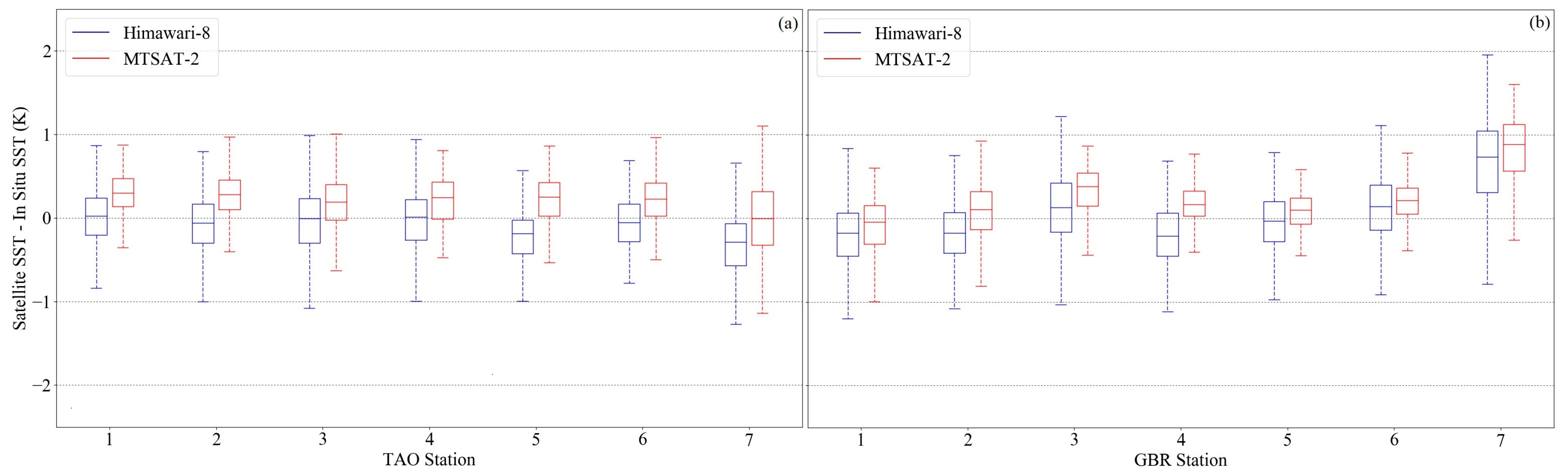
The statistics of the differences between the satellite-derived SST and the in situ temperatures for each of the TAO and GBR stations are shown in Table 4. The statistics of the differences between the satellite-derived SSTs for the Himawari-8 and MTSAT-2 for the entire data set used here are shown in Table 5, and for day and night conditions at the two sets of in situ measurements in Table 6. In general, the mean and median values of the differences are smaller for the Himawari-8 AHI SSTs compared to those of MTSAT-2, but there are exceptions. The standard deviations of the differences do not show the expected improvements in Himawari-8 AHI SSTs compared to those of MTSAT-2, especially at the GBR stations; these are shown graphically in Figure 2 as box-whisker plots. The central bar in the box indicates the median value, and the lower and upper borders of the box represent the first and third quartiles of the distribution of values; the extreme values of the whiskers are the minimum and maximum values, excluding outliers. Outliers were considered those to be beyond 1.5 times the upper and lower quartiles, and are not shown in this and other figures.
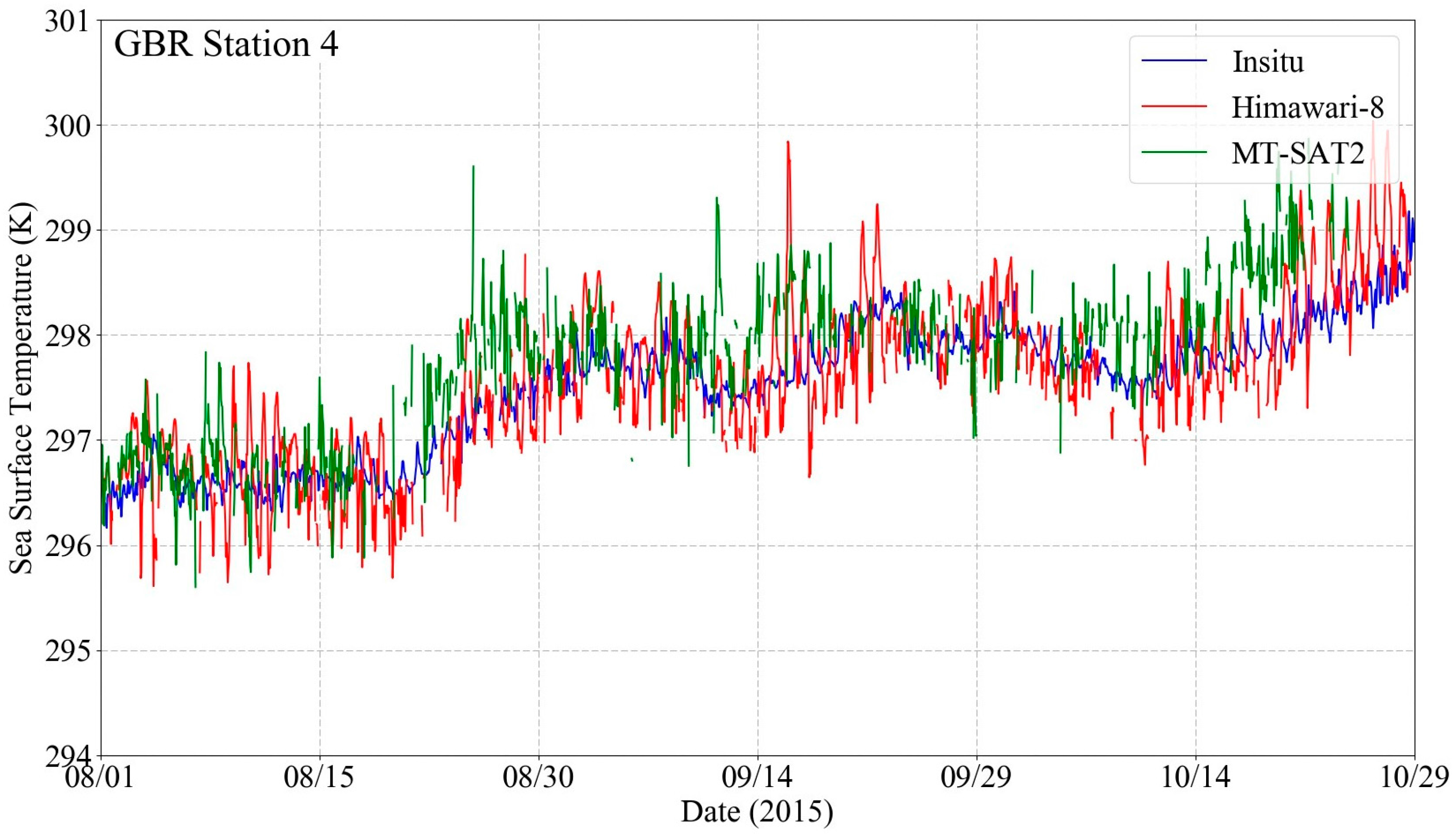
Time series of temperatures measured by the satellites and in situ thermometers for a sample TAO station is shown in Figure 3 and for a sample GBR station in Figure 4. Gaps in the satellite-derived SSTs are where clouds have obscured the surface. At both stations, there is a marked diurnal heating signal in both the in situ sub-surface temperature measurements, and in the satellite-derived SST; this is seen in the times series of measurements at all stations. The days with the largest signals are those with high insolation and low wind speed. In the absence of significant wind-driven vertical mixing, the subsurface temperature signal characteristic of diurnal heating decays with depth [49] and this is revealed in the larger amplitudes of the diurnal temperature signals in the satellite-derived SSTs than in the subsurface temperatures. What is also apparent in these time series is the better agreement between MTSAT-2 SSTs and the subsurface temperatures at night than those derived from Himawari-8, which shows colder SSTs at night. During the day, the Himawari-8 AHI SSTs are generally colder than those of MTSAT-2. The systematic day-night characteristics of the differences between the satellite-derived SSTs and the subsurface temperatures are shown in Figure 5 and Figure 6. The larger median differences, as shown by the bar in the boxes, and the length of the whiskers, between the satellite-derived SSTs and the subsurface temperatures during the day than during the night can be explained by the effects of diurnal heating introducing thermal gradients between the SSTs and the temperatures below.
4. Discussion
The results presented in the previous section show discrepancies that can be explained by many different points of view. This section first introduces the main summary of the results, followed by an explanation of the errors and uncertainties. Since the results show generally smaller SST differences during night-time measurements for both satellites, the diurnal heating effect is an important aspect to investigate. In this discussion, we present data that indeed shows a diurnal signal, along with its effects on the SST differences, and the statistics. Although the diurnal heating effect is one perspective used to help explain discrepancies, other sources such as footprint size and calibration errors are mentioned.
The comparison between the satellite-derived SSTs and the subsurface temperatures show better agreement in the mean for the Himawari-8 AHI SSTs in the areas of both the western TAO array and GBR. For the SST derived from both MTSAT-2 and Himawari-8, results show that the variation within the SST differences decrease during the night. For night-time measurements, the Himawari-8 AHI SSTs show better agreement in the area of the western TAO array. Though the standard deviation of the temperature differences for the MTSAT-2 is smaller than the Himawari-8, the Himawari-8 AHI SSTs are in general more accurate at night. Overall, Himawari-8 shows a mean SST difference of 0.18 K for all stations, while MTSAT-2 shows a mean difference of 0.26 K. The most reduced discrepancy was 0.17 K at GBR Station 4 for the Himawari-8 AHI SSTs. Differences between the stations can be related to the proximity to land, and the depth of the in situ measurement.
The comparisons between SSTs derived from satellite data and in situ measurements are often interpreted as an assessment of the accuracy of the satellite SSTs, but this interpretation assumes the in situ measurements are perfect and accurate, and there are no contributions to the differences from the method of comparison itself [50].
The terms “error” and “uncertainty” have distinct meanings. Error is the difference between a measured value and the true value (generally not known) and uncertainty is the dispersion, or spread, of a group of measurements of the same quantity. Thus, uncertainty is a quantification of the doubt about the measurement result [51,52]. The nature of errors and uncertainties are often described as either systematic or random. Systematic errors and uncertainties can be reduced significantly, and possibly eliminated, through an understanding of their sources and by averaging multiple measurements. In contrast, those that are random cannot be eliminated, but can be reduced by repeating the same measurement, or by taking multiple measurements under the same conditions.
Typically, the accuracy of a satellite-derived SST is expressed as a mean error, or bias, and a scatter, or standard deviation, but these are based on the assumption of a Gaussian distribution. In reality, the symmetry of a Gaussian distribution in studies such as this is rarely seen due to the effects of undetected clouds, which are nearly always colder than the underlying sea surface. This introduces a negative skewness to the distribution. The use of the median and robust standard deviation, which reduces the sensitivity to outliers in the distribution, has become a more accepted method of estimating the central value and dispersion of the differences between satellite-derived and in situ temperatures [53,54,55].
The differences between satellite-derived SSTs and in situ temperature measurements, within acceptable spatial and temporal interval for coincidence [54,56] are not simply an estimate of the accuracy of the satellite SST retrievals as, it is clear that there are multiple contributors to these temperature differences. Some of these contributors include inaccuracies in the in situ measurements and imperfections in the cloud screening algorithms. In addition, because of the finite intervals in space and time between the satellite and the in situ measurement, there is a contribution from the variability in the ocean temperature fields, e.g., [56]. Many of the contributors are independent of each other and can be summed in quadrature to determine the total uncertainty in the differences, which, when combined with the errors and uncertainties in the satellite radiometric measurements can provide the desired estimate of the accuracy for the satellite SST retrievals.
As stated above, the accuracy of the GBR thermometers is better than ±0.1 K and the measurements are recorded with a precision of 0.02 K [11]. The near-surface thermometers on the TRITON moored buoys is given as 0.05 K [44]. Thus, the accuracies of the in situ thermometer, while non-zero, are not likely to be the major cause of the discrepancies.
Given the Robust Standard Deviation (RSD) of the differences between the satellite-derived SSTs and the subsurface temperatures at each of the stations are less sensitive to outliers, these were expected to be smaller than the Standard Deviation, but there are several cases where this is not so. Examination of the histograms of differences revealed that stations where the RSD is larger resulted from distributions that are bimodal, or at least without a clear single peak. Those bimodal histograms may indicate a factor that if identified could be used to determine better estimates of the differences with in situ temperatures, and eventually to better estimates of the accuracies of the satellite-derived SSTs.
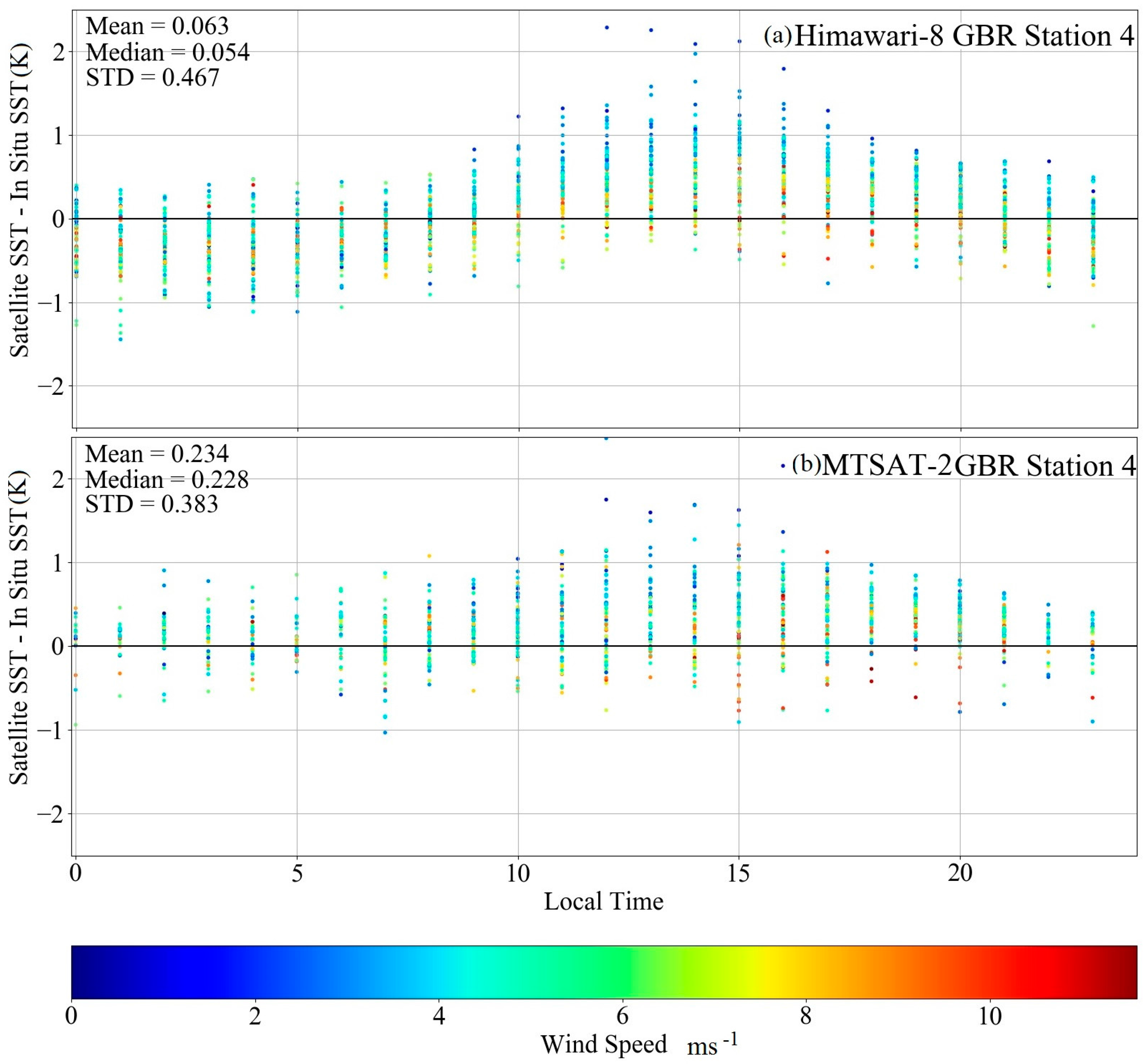
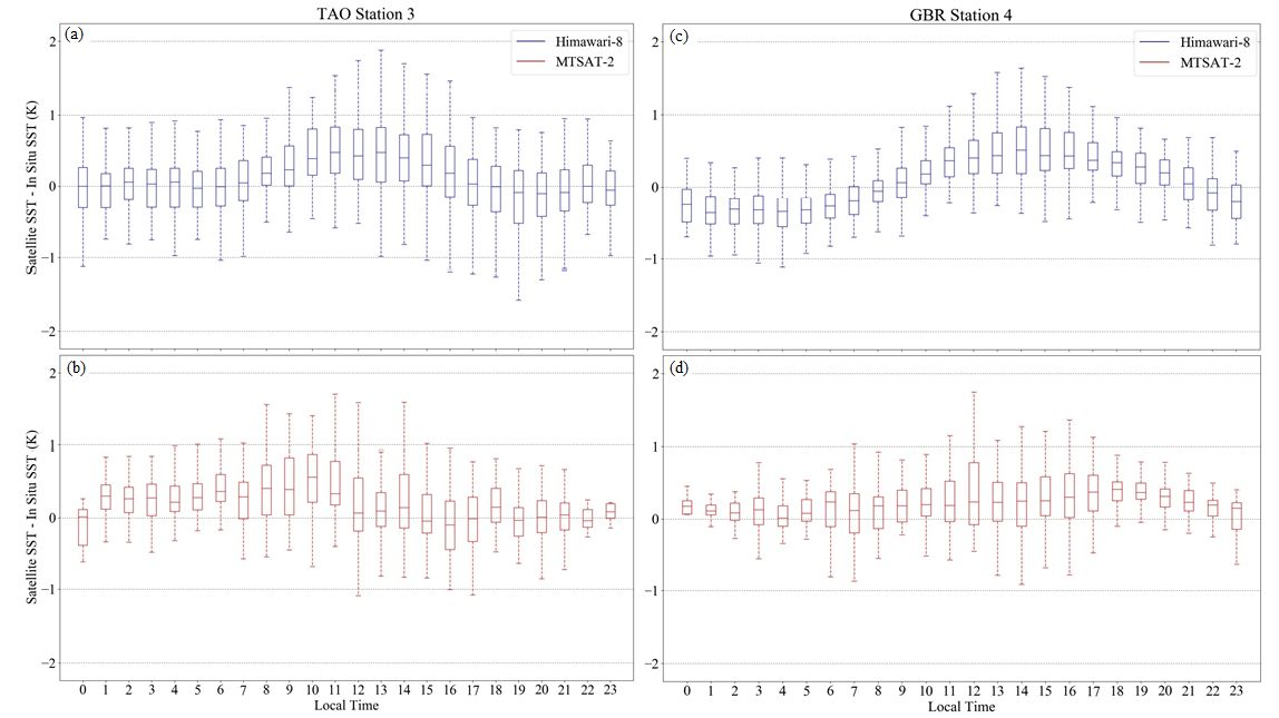
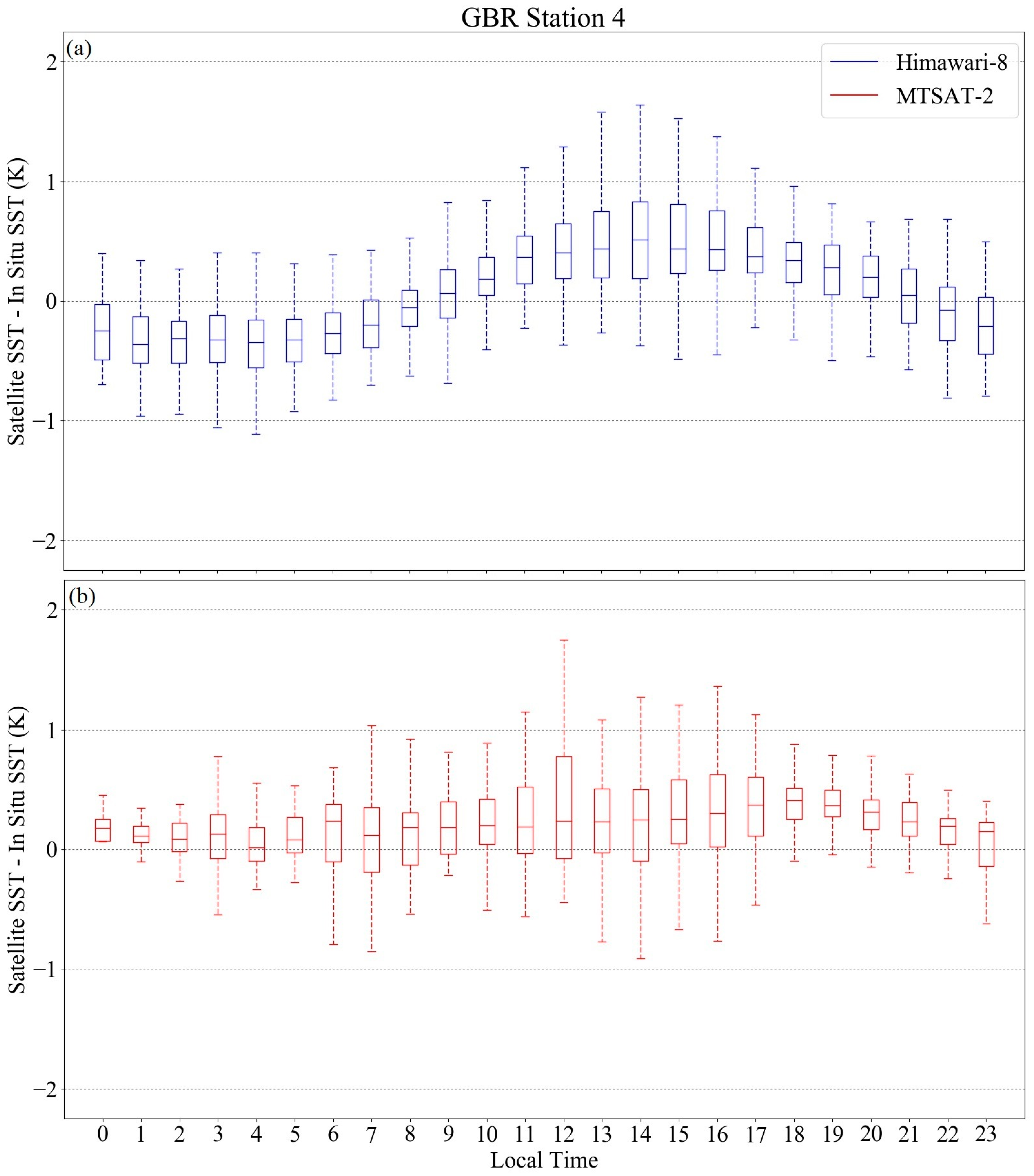
A possible cause of a bimodal distribution in the differences between satellite-derived SSTs and the subsurface temperatures is diurnal heating, and strong diurnal signals in the discrepancies of SST from both satellites are apparent as many stations. Figure 7 shows box-whisker plots of the discrepancies at TAO Station 3, which is quite typical of data from the TAO stations. The characteristics of the discrepancies with Himawari-8 SSTs are better behaved than the comparisons using MTSAT-2 SSTs, in that the pattern is less variable in the median, but the negative median error in the evening and early part of the night is unexpected. The negative median discrepancies in the Himawari-8 comparisons, are more pronounced at the GBR Station 4 (Figure 8).
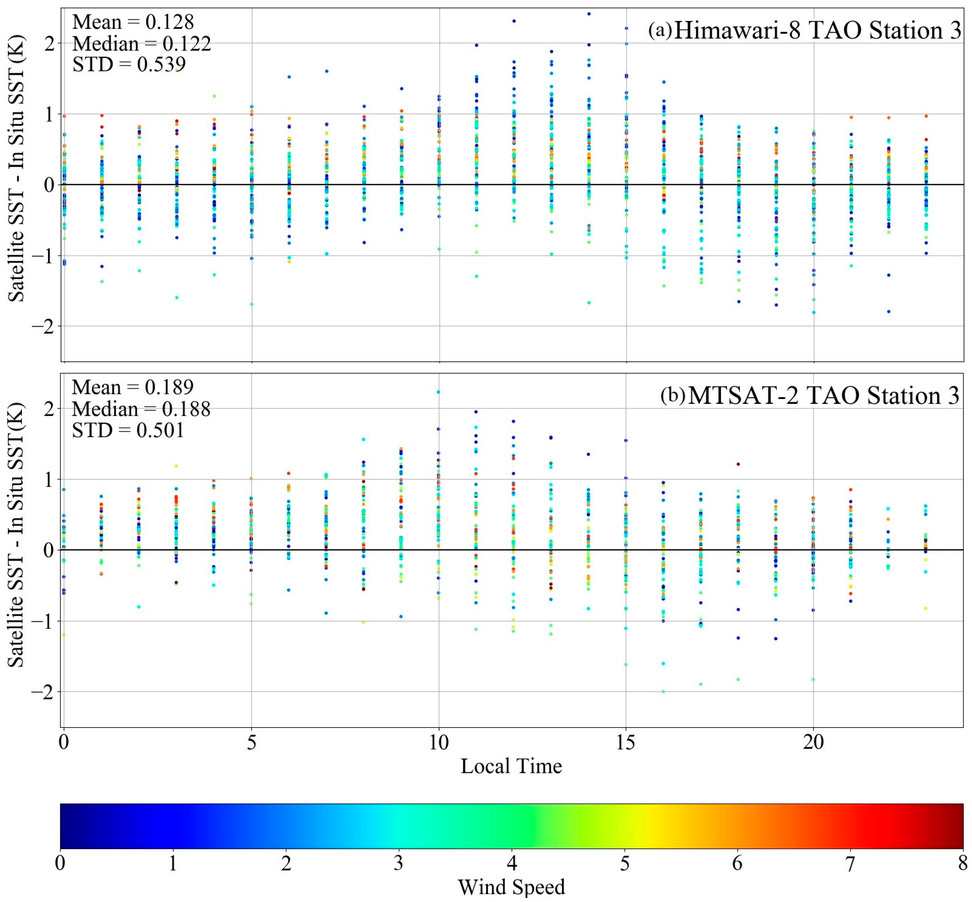
Large temperature differences occurred when there were low wind speeds during the time of the highest insolation around local noon (Figure 9 and Figure 10). This is related to the thermal stratification within the upper ocean. For wind speeds >6 ms−1, the variation within the temperature differences decreased, approaching 0 K, presumably because higher wind speeds mix the upper part of the water column, decreasing the change in the temperature between the SST and the temperature at the depth of the in situ measurements. When the water is well mixed, the difference between measurements will be smaller; making the satellite derived SSTs closer to the in situ measurements and decreasing the discrepancies. SSTs were separated by day and night time to assess the effects of diurnal heating. For Himawari-8, the median temperature difference for each station is generally close to 0 K. The standard deviations in the discrepancies decreased for both satellites at all stations during the night compared to during the day. When comparing night-time differences for both satellites, there is a smaller variation seen within the MTSAT-2 for all in situ stations. Both satellites show better results when the diurnal heating effect is eliminated during the night-time samples and for wind speeds >6 ms−1.
Additional uncertainties within the different mean discrepancies with in situ temperatures for each satellite could be related to the footprint sizes. Though a 5 × 5 pixel array from both satellites were used to compare with the in situ measurements, the differences in resolution causes the array to cover a different total area. The lower spatial resolution of the MTSAT-2 has higher probability of incorporating in situ errors when compared to the spatial resolution of Himawari-8.
Apart from the physical differences between satellite-measured SSTs and buoy measured temperatures at depth, in situ measurements have uncertainties that contribute to the differences. By considering the differences in temperatures measured by pairs of buoys at times of close approach, Emery et al. [57] concluded that the buoy temperatures have an uncertainty of 0.15 K. A subsequent analysis using three-way comparisons between two satellite-derived SSTs and temperatures from drifting buoys, a technique that allows an estimate of the uncertainty to be made for each data set, produced an estimate of the buoy temperature uncertainties of 0.23 K [58]. Other estimates of the uncertainties in temperatures measured from drifting buoys span the range of 0.12 K to 0.67 K [59] (Table 2).
Generally, the in situ measurements are prescreened to remove or note low quality observations. It was previously found that moored buoys had lower measurement uncertainties, whereas drifting buoys and ships introduce more noise [59]. When comparing satellite measurements of SST to in situ measurements, not all of the discrepancies can be assigned to errors in the satellite retrievals. However, the contributions from sources other than the satellite retrieval error should be very similar for both MTSAT-2 and Himawari-8 comparisons with in situ measurements, so the differences in the discrepancies are an indication of the changes in error and uncertainties in the SSTs derived from each satellite.
The data showed that Himawari-8 had an average SST difference of 0.18 ± 0.53 K, with an average median of 0.16 K. The MTSAT-2 had an average SST difference of 0.26 ± 0.48 K, with an average median of 0.27 K. Overall, the Himawari-8 AHI SSTs had smaller discrepancies with the in situ temperatures by an average of 0.08 K. When analyzing only night-time measurements, in which the effects of diurnal heating in the upper ocean should be small, the SST differences had a smaller variation for both satellites at all in situ locations. At times of higher wind speeds, there were also smaller variations within the SST discrepancies.
The large variations in the SST discrepancies were likely related to diurnal thermal stratification that occurs when the water column is not being mixed. High insolation during the day and wind speeds <6 ms−1 are conducive to the formation of thermal stratification [33]. Areas with wind speeds <6 ms−1 cover about 30% of the global ocean surface [33], but in areas of the TRITON moorings the fraction is much larger [60]; the amplitude of diurnal variability of wind speed is generally <0.4 ms−1 [61]. Thus, in the area of the TRITON buoys of the TAO moorings, it is likely that the conditions for the generation of diurnal heating will be met. Thus, the results of this study are consistent with the comparisons being influenced by diurnal heating, leading to an increase in the magnitudes of the SST discrepancies during the day. The expected wind-speed dependence in the diurnal heating signal is apparent in the satellite—in situ temperatures, with smaller discrepancies being seen at higher wind speeds during the day; this is most apparent in Himawari-8 AHI SST comparisons with GBR temperatures (Figure 10). However, distortion of temperature field in the upper ocean by TRITON buoys was found to cause temperature differences at a depth of 0.2 m below the water line on opposite sides of the TRITON buoy of up to 1 K in conditions of large diurnal heating, i.e., a diurnal heating amplitude of 2–3 K [62]. The effects of flow distortion around the buoys are strongly time dependent and thus contribute to the differences found here, but in a manner that is very difficult to quantify.
Inaccuracies in the calibration of the infrared measurements on both MTSAT-2 and Himawari-8 radiometers could lead to bias errors in the satellite-data as errors in the brightness temperatures propagate through the atmospheric correction algorithms. Similarly, brightness temperature errors could compromise the effectiveness of the cloud screening algorithms leading to classification errors allowing pixels with cloud contamination to be misidentified as cloud-free. The objective of the Global Space-based Inter-Calibration System (GSICS) program is to assess the calibration accuracy of thermal infrared (IR) channels of imaging radiometers on geostationary satellites [63]. The reference sensors are the hyperspectral Infrared Atmospheric Sounding Interferometers (IASI) on the European polar-orbiting MetOp satellites [64]. The high resolution spectral measurements of IASI are convolved with the relative spectral response functions of the channels on the satellites on the geostationary satellites to allow comparison between the measurements [65].
GSICS comparisons of MTSAT-2 brightness temperatures and IASI spectral measurements indicate average differences of +0.08 K in the 10.8 μm channel and +0.10 K for the 12 μm channel, with small seasonal variations in the differences [65]. The seasonal fluctuations in the 3.8 μm channel differences are much more pronounced, reaching ~+0.4K around the vernal equinox and somewhat smaller at the autumnal equinox; around the solstices the differences are close to zero [65]. MTSAT-2 is a three-axis stabilized satellite and there is evidence of larger errors about local midnight when the entrance aperture of the imager faces to the sun, and stray solar radiation appears to degrade the calibration of the MTSAT-2 infrared channels [66]. The behavior of these midnight errors are similar to those found for the infrared channels of the imager on the Geostationary Operational Environmental Satellite (GOES -11 and -12; [67]). However, there is no significant evidence of this effect in our analysis.
Comparisons have been made between Himawari-8 AHI brightness temperatures and measurements of IASI on MetOp-A and MetOp-B, of the Atmospheric InfraRed Sounder (AIRS) on Aqua [68] and of the Cross-Track Infrared Sounder (CrIS) on the Suomi-NPP satellite [69]. Preliminary results indicate errors of <±0.1 K for the four bands used in the ACSPO atmospheric correction, Equation (3) [66]. However, the errors are positive for the measurements at 10.4 μm and 11.2 μm, but negative at 8.6 μm and at 12.4 μm. Thus, some of the brightness temperature difference terms in Equation (3) will have small effects on the retrieved temperatures, while those that combine the measurements with errors of opposite signs will make larger contributions. These calibration errors are based on analysis of only one month of data, from early in the Himawari-8 mission, and analysis of longer time series may lead to more confident estimates of the calibration errors.
In a separate study comparing AHI observations and model simulations of brightness temperatures using radiative transfer simulations, Zou, Zhuge and Weng [35] found larger errors in some of the channels. These authors considered a wide geographic area over land as well as ocean, for satellite zenith angles up to 60°, and found a scene dependence of the bias errors, which may be indicative of an imperfect detector non-linearity correction in the calibration process [70]. But, Zou, Zhuge and Weng [35] acknowledge the imperfections in the radiative transfer models could have contributed to the larger estimates of the calibration errors.
5. Conclusions
This study was motivated by an interest to quantify the accuracies of SSTs in the tropical western Pacific Ocean derived from the AHI on Himawari-8, in particular how the SSTs derived from the new sensor have improved compared to those of the heritage sensor on MTSAT-2. The study was facilitated by a period of concurrent operation of both satellites. A particular application of the Himawari-8 AHI SSTs is the contribution they can make to monitoring and studying the health of the corals of the Great Barrier Reef, especially in conditions applying thermal stress to the corals, possibly leading to bleaching and mortality. Earlier work [31] had shown how well SSTs derived from a number of satellite infrared radiometers can represent the temperatures at the depths of the corals, and demonstrated the benefit of SSTs derived from geostationary satellites not only to better resolve the diurnal heating and cooling, but also to reduce obscuration by clouds. Based on the better spectral, temporal, and spatial resolution of the AHI, it was expected to show improved SST accuracy when compared with in situ measurements.
Based on the results of Kramar, Ignatov, Petrenko, Kihai, and Dash [40] we selected AHI SSTs derived using the NOAA ASCPO cloud screening and atmospheric algorithms, and the comparable MTSAT-2 SST data produced by NOAA. Comparison of SSTs from both satellites with subsurface temperatures from thermometers on the TRITON buoys of the TAO moorings and on the Great Barrier Reef, showed the Himawari-8 AHI produces SSTs that agree better with the in situ measurements, but the improvement is relatively modest. The Himawari-8 AHI SSTs appear better, in a qualitative sense, but the quantitative improvements were less pronounced when gross statistics are considered. However, the representation of diurnal variability in the Himawari-8 AHI SSTs is more physical than those in the SSTs from MTSAT-2. In addition to the expected regional bias errors inherent in atmospheric correction algorithms derived for application over larger geographic areas [71], there is evidence in the literature of on-board calibration issues that lead to inaccuracies in the Himawari-8 AHI brightness temperatures that no doubt contribute to the discrepancies reported here.
As more experience is gained with the Himawari-8 AHI data, corrections for the calibration problems will no doubt be found and we can expect improved accuracies in the AHI SSTs; this will benefit many scientific studies in this area. The Himawari-8 AHI SSTs will lead to better forecasts of typhoon activity off Japan’s coast, helping protect the land and its people. In the Great Barrier Reef area, more accurate SSTs will lead to better monitoring the changing ocean temperatures that have harmful effects on the surrounding coral and ecosystems [11].
Acknowledgments
Angela Ditri undertook this research as a summer undergraduate intern at the Ocean Sciences Department of the Rosenstiel School. The GBR temperature time series were provided by the Australian Institute of Marine Science (AIMS), Townsville, Queensland, Australia, and the TRITON mooring data from the Pacific Marine Environmental Laboratory (PMEL) of the National Oceanic and Atmospheric Administration (NOAA). The MTSAT-2 and Himawari-8 AHI SSTs were extracted from the Center for Satellite Applications and Research (STAR) of the National Environmental Satellite, Data, and Information Service (NESDIS) (ftp://ftp.star.nesdis.noaa.gov). This study was funded in part by the NASA Physical Oceanography Program (NNX13AE30G). Angela Ditri is currently supported by the NASA Space Grant College and Fellowship Program (NASA Grant NNX15AI19H).
Author Contributions
Angela Ditri undertook the analysis and contributed to the writing of the manuscript. Peter Minnett conceived and directed the study and wrote most of the manuscript. Yang Liu and Katherine Kilpatrick provided guidance during the analyses. Ajoy Kumar was Angela Ditri’s undergraduate supervisor and provided guidance during the analyses and the writing of the paper.
Conflicts of Interest
The authors declare no conflict of interest.
References
- Robinson, I.S. Measuring the Oceans from Space: The Principles and Methods of Satellite Oceanography; Springer Science & Business Media: Berlin, Germany; New York, NY, USA, 2004; p. 670. [Google Scholar]
- Schneider, T.; Bischoff, T.; Haug, G.H. Migrations and dynamics of the intertropical convergence zone. Nature 2014, 513, 45–53. [Google Scholar] [CrossRef] [PubMed]
- Oki, T.; Kanae, S. Global Hydrological Cycles and World Water Resources. Science 2006, 313, 1068–1072. [Google Scholar] [CrossRef] [PubMed]
- Clement, A.C. The Role of the Ocean in the Seasonal Cycle of the Hadley Circulation. J. Atmos. Sci. 2006, 63, 3351–3365. [Google Scholar] [CrossRef]
- Wada, A.; Chan, J.C.L. Relationship between typhoon activity and upper ocean heat content. Geophys. Res. Lett. 2008, 35, 36–44. [Google Scholar] [CrossRef]
- Benestad, R.E. On tropical cyclone frequency and the warm pool area. Nat. Hazards Earth Syst. Sci. 2009, 9, 635–645. [Google Scholar] [CrossRef]
- Zhang, Q.; Liu, Q.; Wu, L. Tropical Cyclone Damages in China 1983–2006. Bull. Am. Meteorol. Soc. 2009, 90, 489–495. [Google Scholar] [CrossRef]
- Dunn, S.R.; Thomason, J.C.; Le Tissier, M.D.A.; Bythell, J.C. Heat stress induces different forms of cell death in sea anemones and their endosymbiotic algae depending on temperature and duration. Cell Death Differ. 2004, 11, 1213–1222. [Google Scholar] [CrossRef] [PubMed]
- Fitt, W.; Brown, B.; Warner, M.; Dunne, R. Coral bleaching: Interpretation of thermal tolerance limits and thermal thresholds in tropical corals. Coral Reefs 2001, 20, 51–65. [Google Scholar] [CrossRef]
- Rogers, J.S.; Monismith, S.G.; Koweek, D.A.; Torres, W.I.; Dunbar, R.B. Thermodynamics and hydrodynamics in an atoll reef system and their influence on coral cover. Limnol. Oceanogr. 2016, 61, 2191–2206. [Google Scholar] [CrossRef]
- Berkelmans, R.; De’ath, G.; Kininmonth, S.; Skirving, W.J. A comparison of the 1998 and 2002 coral bleaching events on the Great Barrier Reef: Spatial correlation, patterns, and predictions. Coral Reefs 2004, 23, 74–83. [Google Scholar] [CrossRef]
- Hughes, T.P.; Kerry, J.T.; Álvarez-Noriega, M.; Álvarez-Romero, J.G.; Anderson, K.D.; Baird, A.H.; Babcock, R.C.; Beger, M.; Bellwood, D.R.; Berkelmans, R.; et al. Global warming and recurrent mass bleaching of corals. Nature 2017, 543, 373–377. [Google Scholar] [CrossRef] [PubMed]
- Donner, S.D.; Skirving, W.J.; Little, C.M.; Oppenheimer, M.; Hoegh-Guldberg, O.V.E. Global assessment of coral bleaching and required rates of adaptation under climate change. Glob. Chang. Biol. 2005, 11, 2251–2265. [Google Scholar] [CrossRef]
- Kemp, D.W.; Colella, M.A.; Bartlett, L.A.; Ruzicka, R.R.; Porter, J.W.; Fitt, W.K. Life after cold death: Reef coral and coral reef responses to the 2010 cold water anomaly in the Florida Keys. Ecosphere 2016, 7, e01373. [Google Scholar] [CrossRef]
- Hoegh-Guldberg, O.; Fine, M. Low temperatures cause coral bleaching. Coral Reefs 2004, 23, 444. [Google Scholar] [CrossRef]
- Kavousi, J.; Parkinson, J.E.; Nakamura, T. Combined ocean acidification and low temperature stressors cause coral mortality. Coral Reefs 2016, 35, 903–907. [Google Scholar] [CrossRef]
- Langdon, C.; Atkinson, M.J. Effect of elevated pCO2 on photosynthesis and calcification of corals and interactions with seasonal change in temperature/irradiance and nutrient enrichment. J. Geophys. Res. 2005, 110, C09S07. [Google Scholar] [CrossRef]
- Veron, J.E.N.; Devantier, L.M.; Turak, E.; Green, A.L.; Kininmonth, S.; Stafford-Smith, M.; Peterson, N. Delineating the Coral Triangle. Galaxea J. Coral Reef Stud. 2009, 11, 91–100. [Google Scholar] [CrossRef]
- Barber, P.H. The challenge of understanding the Coral Triangle biodiversity hotspot. J. Biogeogr. 2009, 36, 1845–1846. [Google Scholar] [CrossRef]
- Great Barrier Reef Marine Park Authority. Interim Report: 2016 Coral Bleaching Event on the Great Barrier Reef. Preliminary Findings of a Rapid Ecological Impact Assessment and Summary of Environmental Monitoring and Incident Response; Great Barrier Reef Marine Park Authority: Townsville, Australia, 2016; p. 27.
- Cave, D.; Gillis, J. Large Sections of Australia’s Great Reef Are Now Dead, Scientists Find. New York Times, 15 March 2017. [Google Scholar]
- Eakin, C.M.; Liu, G.; Gomez, A.M.; De La Cour, J.L.; Heron, S.F.; Skirving, W.J.; Geiger, E.F.; Tirak, K.V.; Strong, A.E. Global Coral Bleaching 2014–2017: Status and an Appeal for Observations. Reef Encount. 2016, 43, 20–26. [Google Scholar]
- Ainsworth, T.D.; Heron, S.F.; Ortiz, J.C.; Mumby, P.J.; Grech, A.; Ogawa, D.; Eakin, C.M.; Leggat, W. Climate change disables coral bleaching protection on the Great Barrier Reef. Science 2016, 352, 338–342. [Google Scholar] [CrossRef] [PubMed]
- Reverdin, G.; Boutin, J.; Martin, N.; Lourenco, A.; Bouruet-Aubertot, P.; Lavin, A.; Mader, J.; Blouch, P.; Rolland, J.; Gaillard, F.; et al. Temperature Measurements from Surface Drifters. J. Atmos. Ocean. Technol. 2010, 27, 1403–1409. [Google Scholar] [CrossRef]
- Zhang, H.-M.; Reynolds, R.W.; Lumpkin, R.; Molinari, R.; Arzayus, K.; Johnson, M.; Smith, T.M. An Integrated Global Observing System for Sea Surface Temperature Using Satellites and in Situ Data: Research to Operations. Bull. Am. Meteorol. Soc. 2009, 90, 31–38. [Google Scholar] [CrossRef]
- Lumpkin, R.; Özgökmen, T.; Centurioni, L. Advances in the application of surface drifters. Annu. Rev. Mar. Sci. 2017, 9, 59–81. [Google Scholar] [CrossRef] [PubMed]
- Lumpkin, R.; Maximenko, N.; Pazos, M. Evaluating Where and Why Drifters Die. J. Atm. Ocean. Technol. 2012, 29, 300–308. [Google Scholar] [CrossRef]
- Elipot, S.; Lumpkin, R.; Perez, R.C.; Lilly, J.M.; Early, J.J.; Sykulski, A.M. A global surface drifter data set at hourly resolution. J. Geophys. Res. Ocean. 2016, 121, 2937–2966. [Google Scholar] [CrossRef]
- Ando, K.; Kuroda, Y.; Fujii, Y.; Fukuda, T.; Hasegawa, T.; Horii, T.; Ishihara, Y.; Kashino, Y.; Masumoto, Y.; Mizuno, K.; et al. Fifteen years progress of the TRITON array in the Western Pacific and Eastern Indian Oceans. J. Oceanogr. 2017, 73, 403–426. [Google Scholar] [CrossRef]
- Zhu, X.; Minnett, P.J.; Berkelmans, R.; Hendee, J.; Manfrino, C. Diurnal warming in shallow coastal seas: Observations from the Caribbean and Great Barrier Reef regions. Cont. Shelf Res. 2014, 82, 85–98. [Google Scholar] [CrossRef]
- Zhu, X.; Minnett, P.J.; Beggs, H.; Berkelmans, R. Thermal features and diurnal warming at the Great Barrier Reef derived from satellite data. Remote Sens. Environ. 2018. in review. [Google Scholar]
- Donlon, C.J.; Robinson, I.; Casey, K.S.; Vazquez-Cuervo, J.; Armstrong, E.; Arino, O.; Gentemann, C.; May, D.; LeBorgne, P.; Piollé, J.; et al. The Global Ocean Data Assimilation Experiment High-resolution Sea Surface Temperature Pilot Project. Bull. Am. Meteorol. Soc. 2007, 88, 1197–1213. [Google Scholar] [CrossRef]
- Donlon, C.J.; Minnett, P.J.; Gentemann, C.; Nightingale, T.J.; Barton, I.J.; Ward, B.; Murray, J. Toward improved validation of satellite sea surface skin temperature measurements for climate research. J. Clim. 2002, 15, 353–369. [Google Scholar] [CrossRef]
- Kurihara, Y.; Murakami, H.; Kachi, M. Sea surface temperature from the new Japanese geostationary meteorological Himawari-8 satellite. Geophys. Res. Lett. 2016, 43, 1234–1240. [Google Scholar] [CrossRef]
- Zou, X.; Zhuge, X.; Weng, F. Characterization of Bias of Advanced Himawari Imager Infrared Observations from NWP Background Simulations Using CRTM and RTTOV. J. Atmos. Ocean. Technol. 2016, 33, 2553–2567. [Google Scholar] [CrossRef]
- Petrenko, B.; Ignatov, A.; Kihai, Y.; Dash, P. Sensor-Specific Error Statistics for SST in the Advanced Clear-Sky Processor for Oceans. J. Atmos. Ocean. Technol. 2016, 33, 345–359. [Google Scholar] [CrossRef]
- Walton, C.C.; Pichel, W.G.; Sapper, J.F.; May, D.A. The development and operational application of nonlinear algorithms for the measurement of sea surface temperatures with the NOAA polar-orbiting environmental satellites. J. Geophys. Res. 1998, 103, 27999–28012. [Google Scholar] [CrossRef]
- Liang, X.; Ignatov, A.; Kramar, M.; Yu, F. Preliminary Inter-Comparison between AHI, VIIRS and MODIS Clear-Sky Ocean Radiances for Accurate SST Retrievals. Remote Sens. 2016, 8, 203. [Google Scholar] [CrossRef]
- Bessho, K.; Date, K.; Hayashi, M.; Ikeda, A.; Imai, T.; Inoue, H.; Kumagai, Y.; Miyakawa, T.; Murata, H.; Ohno, T.; et al. An Introduction to Himawari-8/9—Japan’s New-Generation Geostationary Meteorological Satellites. J. Meteorol. Soc. Jpn. Ser. II 2016, 94, 151–183. [Google Scholar] [CrossRef]
- Kramar, M.; Ignatov, A.; Petrenko, B.; Kihai, Y.; Dash, P. Near Real Time SST Retrievals from Himawari-8 at NOAA Using ACSPO System. In Proceedings of the Ocean Sensing and Monitoring VIII, Baltimore, MD, USA, 17–21 April 2016; Arnone, R.A., Hou, W.W., Eds.; SPIE: Baltimore, MD, USA, 2016; p. 98270L. [Google Scholar]
- Liang, X.-M.; Ignatov, A.; Kihai, Y. Implementation of the Community Radiative Transfer Model in Advanced Clear-Sky Processor for Oceans and validation against nighttime AVHRR radiances. J. Geophys. Res. Atmos. 2009, 114. [Google Scholar] [CrossRef]
- Brasnett, B.; Surcel-Colan, D. Assimilating Retrievals of Sea Surface Temperature from VIIRS and AMSR2. J. Atmos. Ocean. Technol. 2016, 33, 361–375. [Google Scholar] [CrossRef]
- Xu, F.; Ignatov, A. In situ SST Quality Monitor (iQuam). J. Atmos. Ocean. Technol. 2014, 31, 164–180. [Google Scholar] [CrossRef]
- Kawai, Y.; Kawamura, H.; Tanba, S.; Ando, K.; Yoneyama, K.; Nagahama, N. Validity of sea surface temperature observed with the TRITON buoy under diurnal heating conditions. J. Oceanogr. 2006, 62, 825–838. [Google Scholar] [CrossRef]
- Wolanski, E. Physical Oceanographic Processes of the Great Barrier Reef; CRC Press: Boca Raton, FL, USA, 1994; p. 208. [Google Scholar]
- Zhang, H.; Beggs, H.; Majewski, L.; Wang, X.H.; Kiss, A. Investigating sea surface temperature diurnal variation over the Tropical Warm Pool using MTSAT-1R data. Remote Sens. Environ. 2016, 183, 1–12. [Google Scholar] [CrossRef]
- Gentemann, C.L.; Minnett, P.J. Radiometric measurements of ocean surface thermal variability. J. Geophys. Res. 2008, 113, C08017. [Google Scholar] [CrossRef]
- Saha, S.; Moorthi, S.; Wu, X.; Wang, J.; Nadiga, S.; Tripp, P.; Behringer, D.; Hou, Y.-T.; Chuang, H.-Y.; Iredell, M.; et al. The NCEP Climate Forecast System Version 2. J. Clim. 2014, 27, 2185–2208. [Google Scholar] [CrossRef]
- Ward, B. Near-Surface Ocean Temperature. J. Geophys. Res. 2006, 111, C02005. [Google Scholar] [CrossRef]
- Corlett, G.K.; Merchant, C.J.; Minnett, P.J.; Donlon, C.J. Assessment of Long-Term Satellite Derived Sea Surface Temperature Records. In Experimental Methods in the Physical Sciences, Optical Radiometry for Ocean Climate Measurements; Zibordi, G., Donlon, C.J., Parr, A.C., Eds.; Academic Press: Cambridge, MA, USA, 2014; Volume 47, pp. 639–677. [Google Scholar]
- Working Group 1 of the Joint Committee for Guides in Metrology. Evaluation of Measurement Data—Guide to the Expression of Uncertainty in Measurement; BIPM: Sèvres, France, 2008; p. 134. [Google Scholar]
- Bell, S. A Beginner’s Guide to Uncertainty of Measurement; National Physical Laboratory: Teddington, UK, 2001; p. 41. [Google Scholar]
- Kilpatrick, K.A.; Podestá, G.; Walsh, S.; Williams, E.; Halliwell, V.; Szczodrak, M.; Brown, O.B.; Minnett, P.J.; Evans, R. A decade of sea surface temperature from MODIS. Remote Sens. Environ. 2015, 165, 27–41. [Google Scholar] [CrossRef]
- Embury, O.; Merchant, C.J.; Corlett, G.K. A reprocessing for climate of sea surface temperature from the along-track scanning radiometers: Initial validation, accounting for skin and diurnal variability effects. Remote Sens. Environ. 2012, 116, 62–78. [Google Scholar] [CrossRef]
- Merchant, C.J.; Harris, A.R. Toward the elimination of bias in satellite retrievals of skin sea surface temperature. 2: Comparison with in situ measurements. J. Geophys. Res. 1999, 104, 23579–23590. [Google Scholar] [CrossRef]
- Minnett, P.J. Consequences of sea surface temperature variability on the validation and applications of satellite measurements. J. Geophys. Res. 1991, 96, 18475–18489. [Google Scholar] [CrossRef]
- Emery, W.J.; Baldwin, D.J.; Schlüssel, P.; Reynolds, R.W. Accuracy of in situ sea surface temperatures used to calibrate infrared satellite measurements. J. Geophys. Res. 2001, 106, 2387–2405. [Google Scholar] [CrossRef]
- O'Carroll, A.G.; Eyre, J.R.; Saunders, R.W. Three-Way Error Analysis between AATSR, AMSR-E, and In Situ Sea Surface Temperature Observations. J. Atmos. Ocean. Technol. 2008, 25, 1197–1207. [Google Scholar] [CrossRef]
- Kennedy, J.J. A review of uncertainty in in situ measurements and data sets of sea surface temperature. Rev. Geophys. 2014, 51, 1–32. [Google Scholar] [CrossRef]
- Woods, S.; Minnett, P.J.; Gentemann, C.L.; Bogucki, D. Influence of the oceanic cool skin layer on global air–sea CO2 flux estimates. Remote Sens. Environ. 2014, 145, 15–24. [Google Scholar] [CrossRef]
- Dai, A.; Deser, C. Diurnal and semidiurnal variations in global surface wind and divergence fields. J. Geophys. Res. Atmos. 1999, 104, 31109–31125. [Google Scholar]
- Kawai, Y.; Ando, K.; Kawamura, H. Distortion of Near-Surface Seawater Temperature Structure by a Moored-Buoy Hull and Its Effect on Skin Temperature and Heat Flux Estimates. Sensors 2009, 9, 6119–6130. [Google Scholar] [CrossRef] [PubMed]
- Goldberg, M.; Ohring, G.; Butler, J.; Cao, C.; Datla, R.; Doelling, D.; Gärtner, V.; Hewison, T.; Iacovazzi, B.; Kim, D.; et al. The Global Space-Based Inter-Calibration System. Bull. Am. Meteorol. Soc. 2011, 92, 467–475. [Google Scholar] [CrossRef]
- Blumstein, D.; Chalon, G.; Carlier, T.; Buil, C.; Hebert, P.; Maciaszek, T.; Ponce, G.; Phulpin, T.; Tournier, B.; Simeoni, D.; et al. IASI Instrument: Technical Overview and Measured Performances. In Proceedings of the Optical Science and Technology, the SPIE 49th Annual Meeting, Denver, CO, USA, 2–6 August 2004; Strojnik, M., Ed.; Volume 5543, pp. 196–207. [Google Scholar]
- Hewison, T.J.; Wu, X.; Yu, F.; Tahara, Y.; Hu, X.; Kim, D.; Koenig, M. GSICS inter-calibration of infrared channels of geostationary imagers using Metop/IASI. IEEE Trans. Geosci. Remote Sens. 2013, 51, 1160–1170. [Google Scholar] [CrossRef]
- Okuyama, A.; Andou, A.; Date, K.; Hoasaka, K.; Mori, N.; Murata, H.; Tabata, T.; Takahashi, M.; Yoshino, R.; Bessho, K. Preliminary Validation of Himawari-8/AHI Navigation and Calibration. In Proceedings of the Earth Observing Systems XX, San Diego, CA, USA, 10–13 August 2015; Butler, J.J., Jack, X., Gu, X., Eds.; p. 96072E. [Google Scholar]
- Yu, F.; Wu, X.; Raja, M.R.V.; Li, Y.; Wang, L.; Goldberg, M. Diurnal and scan angle variations in the calibration of GOES imager infrared channels. IEEE Trans. Geosci. Remote Sens. 2013, 51, 671–683. [Google Scholar] [CrossRef]
- Aumann, H.H.; Chahine, M.T.; Gautier, C.; Goldberg, M.D.; Kalnay, E.; McMillin, L.M.; Revercomb, H.; Rosenkranz, P.W.; Smith, W.L.; Staelin, D.H.; et al. AIRS/AMSU/HSB on the Aqua Mission: Design, science objectives, data products, and processing systems. IEEE Trans. Geosci. Remote Sens. 2003, 41, 253–264. [Google Scholar] [CrossRef]
- Han, Y.; Revercomb, H.; Cromp, M.; Gu, D.; Johnson, D.; Mooney, D.; Scott, D.; Strow, L.; Bingham, G.; Borg, L.; et al. Suomi NPP CrIS measurements, sensor data record algorithm, calibration and validation activities, and record data quality. J. Geophys. Res. Atmos. 2013, 118, 12734–12748. [Google Scholar] [CrossRef]
- Saunders, R.W.; Blackmore, T.A.; Candy, B.; Francis, P.N.; Hewison, T.J. Monitoring Satellite Radiance Biases Using NWP Models. IEEE Trans. Geosci. Remote Sens. 2013, 51, 1124–1138. [Google Scholar] [CrossRef]
- Minnett, P.J. The regional optimization of infrared measurements of sea-surface temperature from space. J. Geophys. Res. 1990, 95, 13497–13510. [Google Scholar] [CrossRef]
Figure 1.
Locations of in situ stations providing subsurface temperatures for this study.

Figure 2.
Box plots for the temperature difference between the satellite-derived SST and subsurface temperature at each TAO mooring (a) and GBR station (b). Blue boxes and whiskers represent the temperature differences for the Himawari-8 SSTs. Red represents the temperature differences for the MTSAT-2 SSTs. Outliers are not plotted.
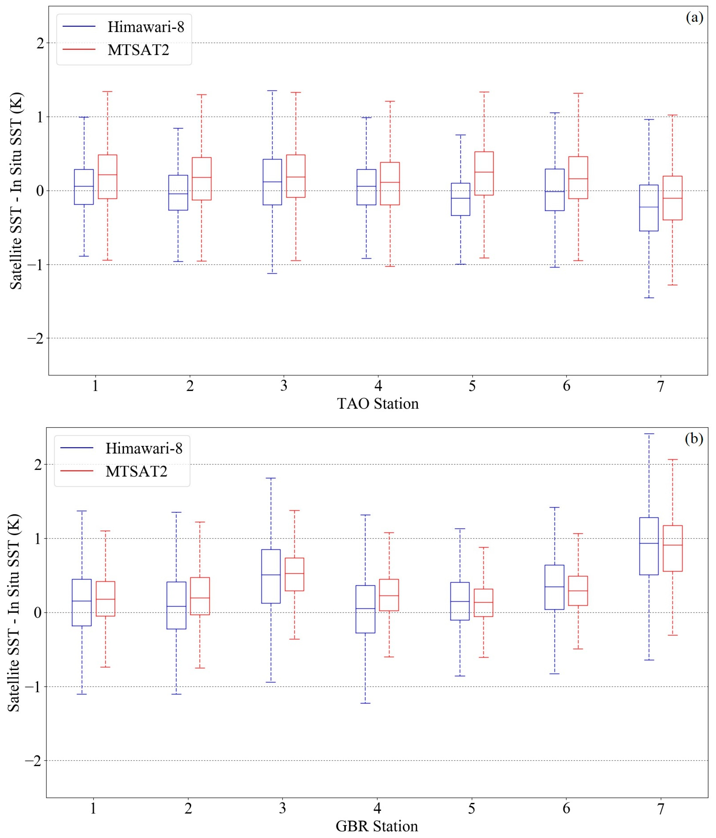
Figure 3.
Time series of near-surface temperature measurements at the TAO-1 mooring at 0°N, 147°E (blue) and the satellite-derived SST from Himawari-8 (red) and MTSAT-2 (green).
Figure 3.
Time series of near-surface temperature measurements at the TAO-1 mooring at 0°N, 147°E (blue) and the satellite-derived SST from Himawari-8 (red) and MTSAT-2 (green).
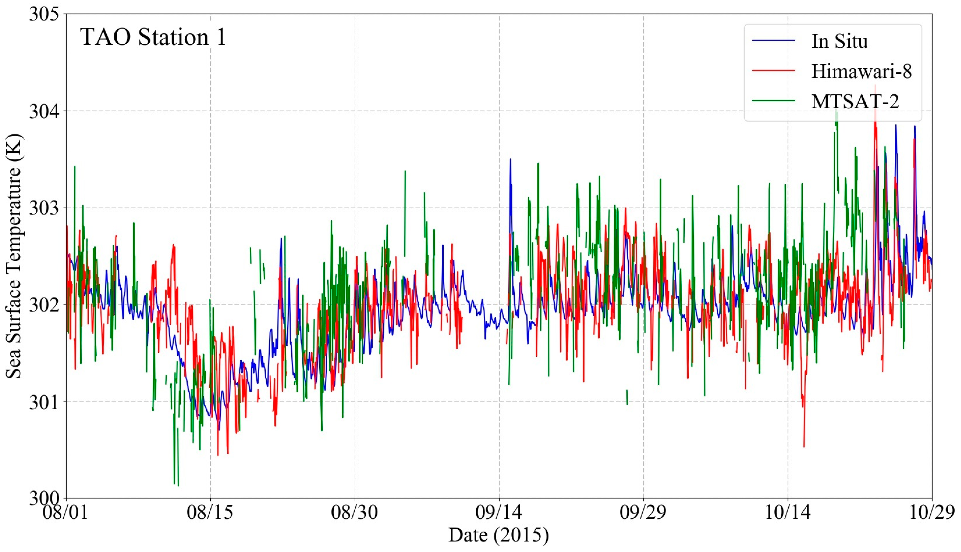
Figure 4.
Time series of temperature measurements at the depth (1.9 m) of the corals GBR-4 station at 18.49°S, 146.87°E (blue), and the satellite-derived SST from Himawari-8 (red) and MTSAT-2 (green).
Figure 4.
Time series of temperature measurements at the depth (1.9 m) of the corals GBR-4 station at 18.49°S, 146.87°E (blue), and the satellite-derived SST from Himawari-8 (red) and MTSAT-2 (green).

Figure 5.
Box plots of the differences between satellite and in situ temperatures for day (blue) and night (red). The top row (a,b) is for MTSAT-2 SSTs, and the bottom row (c,d) for Himawari-8. The left column (a,c) is for the TAO moorings and the right column (b,d) for the GBR stations. Outliers are not shown.
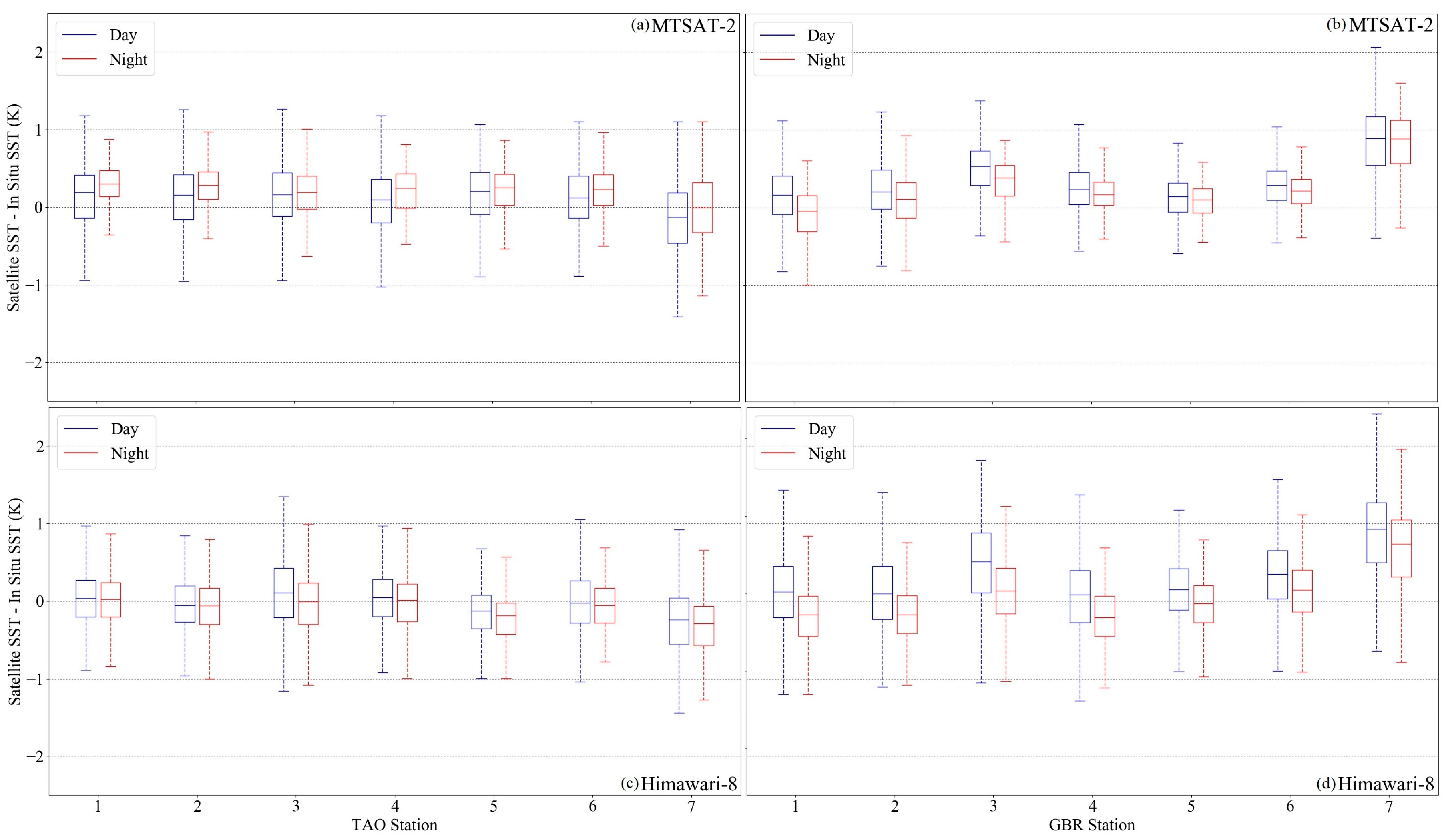
Figure 6.
Box plots of the night-time differences for the satellite-derived SST and the in situ temperatures for Himarari-8 (blue) and MTSAT-2 (red). TAO moorings are at left (a); GBR stations at right (b). Outliers are not plotted.
Figure 6.
Box plots of the night-time differences for the satellite-derived SST and the in situ temperatures for Himarari-8 (blue) and MTSAT-2 (red). TAO moorings are at left (a); GBR stations at right (b). Outliers are not plotted.

Figure 7.
Box plots of the hourly differences between the satellite-derived SSTs and the subsurface temperatures measured at TAO Station 3 at 2°N, 137°E. Differences of SSTs from Hiawari-8 are shown in blue in (a), and from MTSAT-2 in red in (b). Outliers are not plotted. The data are of best quality level from 1 August 2015–31 October 2015.
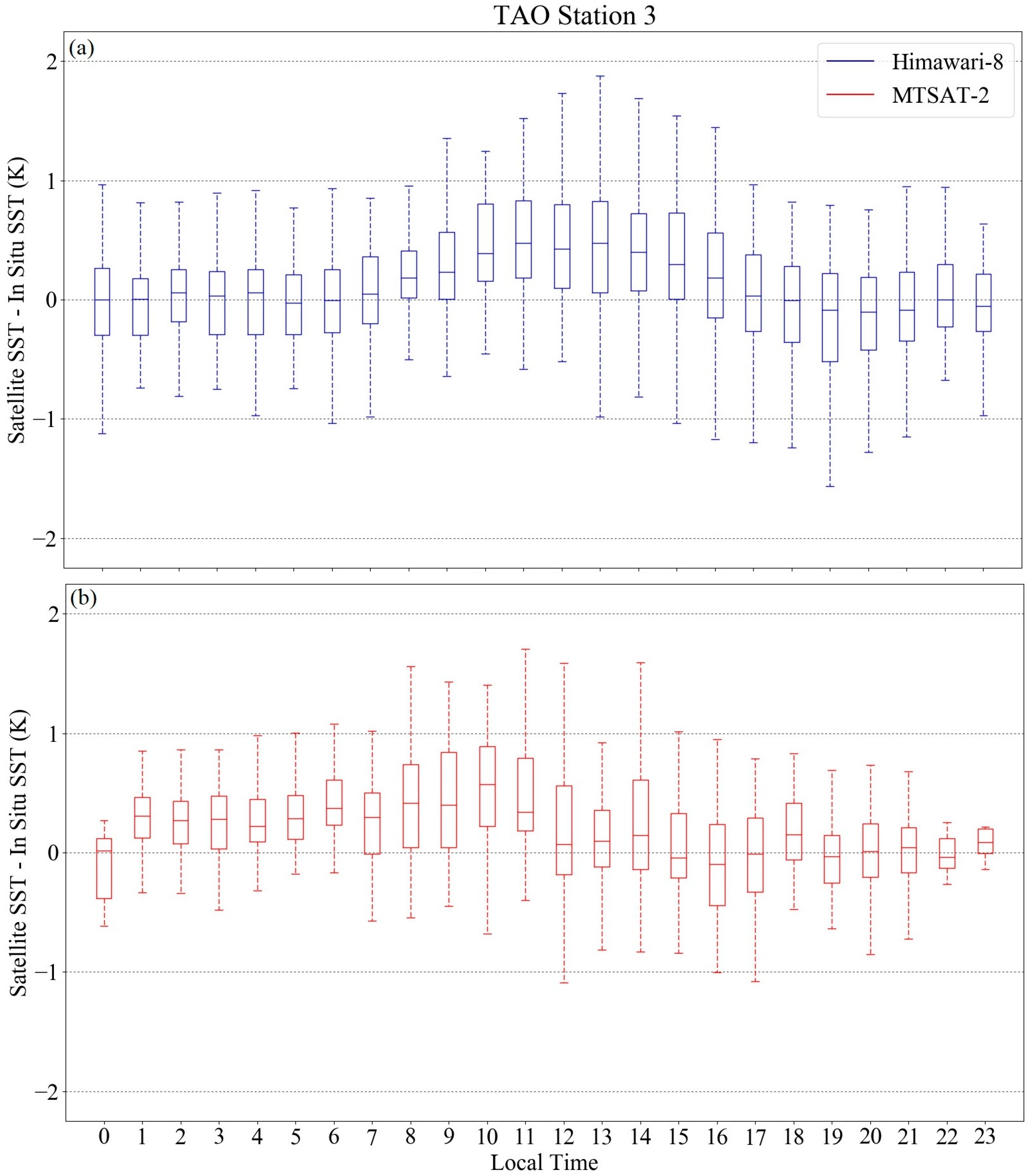
Figure 8.
As Figure 7, but for GBR Station 4 at 18.49°S, 146.87°E with in situ temperatures measured at a depth of 1.9 m. Differences of SSTs from Hiawari-8 are shown in blue in (a), and from MTSAT-2 in red in (b).
Figure 8.
As Figure 7, but for GBR Station 4 at 18.49°S, 146.87°E with in situ temperatures measured at a depth of 1.9 m. Differences of SSTs from Hiawari-8 are shown in blue in (a), and from MTSAT-2 in red in (b).

Figure 9.
Differences between satellite-derived SST and in situ temperatures for each hour of the day at the TAO mooring 3 at 2°N, 137°E. The colors represent wind speed in ms−1. The dots correspond to highest quality data from 1 August 2015–31 October 2015. The top panel is for SSTs from Himawari-8 and the lower panel for SSTs from MTSAT-2.

Figure 10.
As Figure 9 but for GBR Station 4 at 18.49°S, 146.87°E with in situ temperatures measured at a depth of 1.9 m.
Figure 10.
As Figure 9 but for GBR Station 4 at 18.49°S, 146.87°E with in situ temperatures measured at a depth of 1.9 m.

Table 1.
Details of satellite data used in this study.
| Satellite Name | Spatial Resolution | Temporal Resolution | Position | No. of Spectral Bands | Operation Period |
|---|---|---|---|---|---|
| MTSAT-2 | 4 km | Hourly | 0°N, 145.0°E | 5 | 2010 to 2015 |
| Himawari-8 | 2 km | 10 min | 0°N, 140.7°E | 16 | 2015 to 2022 |
Table 2.
Locations and depth of in situ measurements.
| Station | Lat | Lon | Thermometer Depth |
|---|---|---|---|
| TAO 1 | 0°N | 147°E | 1.5 m |
| TAO 2 | 0°N | 156°E | 1.5 m |
| TAO 3 | 2°N | 137°E | 1.5 m |
| TAO 4 | 2°N | 147°E | 1.5 m |
| TAO 5 | 8°N | 137°E | 1.5 m |
| TAO 6 | 2°N | 156°E | 1.5 m |
| TAO 7 | 2°S | 156°E | 1.5 m |
| GBR 1 | 21.87°S | 152.52°E | 10.4 m |
| GBR 2 | 16.64°S | 146.11°E | 7.0 m |
| GBR 3 | 18.83°S | 147.63°E | 3.3 m |
| GBR 4 | 18.49°S | 146.87°E | 1.9 m |
| GBR 5 | 21.03°S | 150.85°E | 7.1 m |
| GBR 6 | 21.41°S | 151.64°E | 7.1 m |
| GBR 7 | 21.11°S | 152.55°E | 8.3 m |
Table 3.
Sampling and averaging summary for generating matchups between satellite and in situ measurements.
Table 3.
Sampling and averaging summary for generating matchups between satellite and in situ measurements.
| GBR | TAO | ||
|---|---|---|---|
| MTSAT-2 | 1 h sampling interval | In situ temperatures within the hour following the satellite SST measurement were averaged. | Hourly in situ temperatures were paired with corresponding hour of the satellite SST. |
| Himawari-8 AHI | 10 min sampling interval | Although same sampling intervals, they were not synchronized. In situ temperatures were interpolated to satellite sample times. | Satellite SST samples that were within the hour of the in situ sample were averaged. |
Table 4.
Statistics of satellite Sea-Surface Temperature (SST)—in situ temperatures (K). Upper row for each station is for Himawari-8 SSTs, and the lower row for MTSAT-2 SSTs.
Table 4.
Statistics of satellite Sea-Surface Temperature (SST)—in situ temperatures (K). Upper row for each station is for Himawari-8 SSTs, and the lower row for MTSAT-2 SSTs.
| Station | θ | N | N of Outliers | Min | Max | Day Mean | Night Mean | Day Median | Night Median | Day STD | Night STD | Day RSD | Night RSD |
|---|---|---|---|---|---|---|---|---|---|---|---|---|---|
| TAO 1 | 7° | 1464 | 19 | −1.294 | 1.759 | 0.034 | 0.009 | 0.033 | 0.022 | 0.368 | 0.353 | 0.349 | 0.330 |
| 2° | 848 | 15 | −1.385 | 1.670 | 0.141 | 0.268 | 0.194 | 0.300 | 0.447 | 0.341 | 0.409 | 0.250 | |
| TAO 2 | 18° | 909 | 6 | −1.045 | 0.977 | −0.048 | −0.058 | −0.057 | −0.060 | 0.336 | 0.324 | 0.349 | 0.349 |
| 13° | 480 | 13 | −1.480 | 1.970 | 0.113 | 0.224 | 0.157 | 0.283 | 0.453 | 0.353 | 0.427 | 0.263 | |
| TAO 3 | 5° | 1768 | 64 | −1.810 | 2.605 | 0.119 | −0.036 | 0.105 | −0.007 | 0.554 | 0.439 | 0.473 | 0.395 |
| 10° | 1105 | 45 | −2.000 | 2.230 | 0.160 | 0.165 | 0.161 | 0.189 | 0.500 | 0.358 | 0.413 | 0.315 | |
| TAO 4 | 8° | 1255 | 46 | −2.039 | 1.419 | 0.005 | −0.037 | 0.046 | 0.010 | 0.441 | 0.420 | 0.355 | 0.362 |
| 3° | 639 | 22 | −1.565 | 2.020 | 0.053 | 0.197 | 0.094 | 0.243 | 0.467 | 0.321 | 0.416 | 0.331 | |
| TAO 5 | 10° | 1004 | 26 | −1.791 | 0.758 | −0.158 | −0.233 | −0.124 | −0.184 | 0.359 | 0.327 | 0.319 | 0.299 |
| 13° | 550 | 23 | −1.535 | 1.833 | 0.181 | 0.226 | 0.203 | 0.252 | 0.457 | 0.291 | 0.400 | 0.295 | |
| TAO 6 | 18° | 1008 | 6 | −1.286 | 2.520 | −0.011 | −0.047 | −0.027 | −0.055 | 0.385 | 0.346 | 0.403 | 0.333 |
| 13° | 507 | 20 | −1.980 | 1.825 | 0.096 | 0.220 | 0.121 | 0.225 | 0.489 | 0.292 | 0.399 | 0.295 | |
| TAO 7 | 18° | 880 | 14 | −2.184 | 0.967 | −0.279 | −0.310 | −0.243 | −0.286 | 0.498 | 0.431 | 0.441 | 0.374 |
| 13° | 458 | 14 | −2.240 | 1.530 | −0.179 | −0.025 | −0.128 | −0.008 | 0.513 | 0.423 | 0.478 | 0.474 | |
| GBR 1 | 29° | 1886 | 58 | −2.523 | 2.003 | 0.089 | −0.239 | 0.121 | −0.177 | 0.545 | 0.497 | 0.491 | 0.383 |
| 27° | 1136 | 46 | −2.271 | 1.763 | 0.147 | −0.137 | 0.159 | −0.042 | 0.437 | 0.429 | 0.367 | 0.343 | |
| GBR2 | 20° | 1844 | 21 | −1.300 | 2.873 | 0.117 | −0.163 | 0.095 | −0.174 | 0.490 | 0.353 | 0.504 | 0.360 |
| 19° | 977 | 38 | −1.513 | 2.174 | 0.231 | 0.079 | 0.205 | 0.108 | 0.433 | 0.380 | 0.375 | 0.341 | |
| GBR3 | 23° | 1980 | 22 | −1.665 | 2.922 | 0.474 | 0.116 | 0.507 | 0.132 | 0.545 | 0.447 | 0.575 | 0.437 |
| 22° | 1260 | 46 | −1.625 | 3.007 | 0.512 | 0.298 | 0.530 | 0.382 | 0.402 | 0.357 | 0.327 | 0.293 | |
| GBR 4 | 23° | 1838 | 20 | −1.445 | 2.287 | 0.082 | −0.193 | 0.086 | −0.208 | 0.483 | 0.365 | 0.498 | 0.381 |
| 22° | 1138 | 44 | −1.037 | 2.485 | 0.249 | 0.155 | 0.236 | 0.169 | 0.380 | 0.265 | 0.306 | 0.222 | |
| GBR 5 | 27° | 1996 | 19 | −1.428 | 1.252 | 0.133 | −0.050 | 0.150 | −0.030 | 0.381 | 0.349 | 0.395 | 0.356 |
| 25° | 1334 | 41 | −1.365 | 1.578 | 0.122 | 0.069 | 0.141 | 0.101 | 0.311 | 0.251 | 0.273 | 0.235 | |
| GBR6 | 28° | 1944 | 17 | −1.304 | 1.700 | 0.334 | 0.127 | 0.346 | 0.143 | 0.433 | 0.388 | 0.460 | 0.400 |
| 26° | 1163 | 38 | −1.609 | 1.360 | 0.280 | 0.187 | 0.288 | 0.218 | 0.331 | 0.288 | 0.282 | 0.232 | |
| GBR 7 | 28° | 1787 | 9 | −0.821 | 2.451 | 0.885 | 0.675 | 0.930 | 0.736 | 0.548 | 0.530 | 0.575 | 0.548 |
| 26° | 954 | 7 | −1.325 | 2.379 | 0.849 | 0.829 | 0.894 | 0.889 | 0.449 | 0.385 | 0.466 | 0.414 |
θ is the satellite zenith angle; N is the number of matchups (Column 3) and of outliers (Column 4); RSD is Robust Standard Deviation.
Table 5.
Statistics of satellite SST—in situ temperatures (K).
| N | Mean | Median | STD | RSD | |
|---|---|---|---|---|---|
| Himawari-8 | 21563 | 0.180 | 0.155 | 0.534 | 0.492 |
| MTSAT-2 | 12549 | 0.261 | 0.269 | 0.480 | 0.402 |
Table 6.
Statistics of satellite SST—in situ temperatures (K) for day and night conditions at the positions of the Tropical Atmosphere Ocean (TAO) moorings and the Great Barrier Reef (GBR) stations.
Table 6.
Statistics of satellite SST—in situ temperatures (K) for day and night conditions at the positions of the Tropical Atmosphere Ocean (TAO) moorings and the Great Barrier Reef (GBR) stations.
| N | Day Mean | Night Mean | Day Median | Night Median | Day STD | Night STD | Day RSD | Night RSD | |
|---|---|---|---|---|---|---|---|---|---|
| TAO/Himawari-8 | 8288 | −0.022 | −0.086 | −0.015 | −0.075 | 0.454 | 0.399 | 0.393 | 0.366 |
| TAO/MTSAT-2 | 4587 | 0.099 | 0.189 | 0.137 | 0.230 | 0.487 | 0.351 | 0.420 | 0.321 |
| GBR/Himawari-8 | 13,275 | 0.299 | 0.037 | 0.283 | 0.006 | 0.561 | 0.510 | 0.543 | 0.461 |
| GBR/MTSAT-2 | 7962 | 0.329 | 0.196 | 0.302 | 0.189 | 0.452 | 0.424 | 0.392 | 0.325 |
© 2018 by the authors. Licensee MDPI, Basel, Switzerland. This article is an open access article distributed under the terms and conditions of the Creative Commons Attribution (CC BY) license (http://creativecommons.org/licenses/by/4.0/).
Share and Cite
MDPI and ACS Style
Ditri, A.L.; Minnett, P.J.; Liu, Y.; Kilpatrick, K.; Kumar, A. The Accuracies of Himawari-8 and MTSAT-2 Sea-Surface Temperatures in the Tropical Western Pacific Ocean. Remote Sens. 2018, 10, 212. https://doi.org/10.3390/rs10020212
AMA Style
Ditri AL, Minnett PJ, Liu Y, Kilpatrick K, Kumar A. The Accuracies of Himawari-8 and MTSAT-2 Sea-Surface Temperatures in the Tropical Western Pacific Ocean. Remote Sensing. 2018; 10(2):212. https://doi.org/10.3390/rs10020212
Chicago/Turabian StyleDitri, Angela L., Peter J. Minnett, Yang Liu, Katherine Kilpatrick, and Ajoy Kumar. 2018. "The Accuracies of Himawari-8 and MTSAT-2 Sea-Surface Temperatures in the Tropical Western Pacific Ocean" Remote Sensing 10, no. 2: 212. https://doi.org/10.3390/rs10020212
Note that from the first issue of 2016, this journal uses article numbers instead of page numbers. See further details here.