Retrieval of Reflected Shortwave Radiation at the Top of the Atmosphere Using Himawari-8/AHI Data
by
 ,
,
Sang-Ho Lee
1,2, 
Bu-Yo Kim
1,2,
Kyu-Tae Lee
1,2,*,
Il-Sung Zo
2,
Hyun-Seok Jung
1,2 and
Se-Hun Rim
1,2 1
Department of Atmospheric and Environmental Sciences, Gangneung-Wonju National University, 7, Jukheon-gil, Gangneung-si, Gangwon-do 25457, Korea
2
Research Institute for Radiation-Satellite, Gangneung-Wonju National University, 7, Jukheon-gil, Gangneung-si, Gangwon-do 25457, Korea
*
Author to whom correspondence should be addressed.
Remote Sens. 2018, 10(2), 213; https://doi.org/10.3390/rs10020213
Submission received: 30 November 2017
/
Revised: 8 January 2018
/
Accepted: 25 January 2018
/
Published: 1 February 2018
(This article belongs to the Special Issue Solar Radiation, Modelling and Remote Sensing)
Abstract
:This study developed a retrieval algorithm for reflected shortwave radiation at the top of the atmosphere (RSR). This algorithm is based on Himawari-8/AHI (Advanced Himawari Imager) whose sensor characteristics and observation area are similar to the next-generation Geostationary Korea Multi-Purpose Satellite/Advanced Meteorological Imager (GK-2A/AMI). This algorithm converts the radiance into reflectance for six shortwave channels and retrieves the RSR with a regression coefficient look-up-table according to geometry of the solar-viewing (solar zenith angle, viewing zenith angle, and relative azimuth angle) and atmospheric conditions (surface type and absence/presence of clouds), and removed sun glint with high uncertainty. The regression coefficients were calculated using numerical experiments from the radiative transfer model (SBDART), and ridge regression for broadband albedo at the top of the atmosphere (TOA albedo) and narrowband reflectance considering anisotropy. The retrieved RSR were validated using Terra, Aqua, and S-NPP/CERES data on the 15th day of every month from July 2015 to February 2017. The coefficient of determination (R2) between AHI and CERES for scene analysis was higher than 0.867 and the Bias and root mean square error (RMSE) were −21.34–5.52 and 51.74–59.28 Wm−2. The R2, Bias, and RMSE for the all cases were 0.903, −2.34, and 52.12 Wm−2, respectively.
Keywords:
Himawari-8/Advanced Meteorological Imager (Himawari-8/AHI); Geostationary Korea Multi-Purse Satellite/Advanced Meteorological Imager (GK-2A/AMI); broadband albedo at the top of the atmosphere (TOA albedo); reflected shortwave radiation at the top of the atmosphere (RSR); Clouds and the Earth Radiant Energy System (CERES)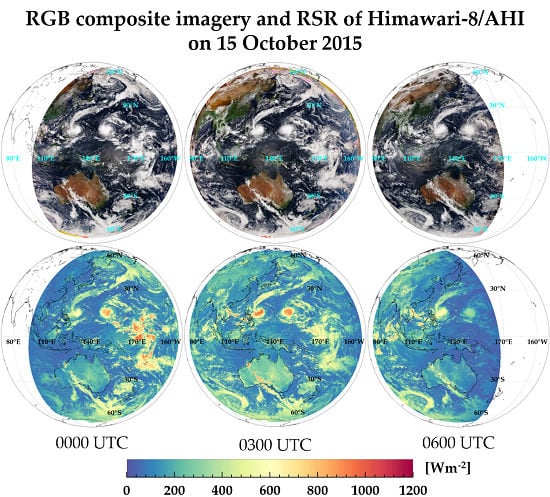
1. Introduction
Reflected shortwave radiation at the top of the atmosphere (RSR) is affected by the surface characteristics (15%); atmosphere gases such as aerosols, vapors, etc. (20%); and clouds (65%) [1]. In particular, a clear-sky area is greatly influenced by short-wavelength ultraviolet and near-infrared rays depending on surface characteristics, whereas a cloudy-sky area is affected more by the cloud properties [2]. In addition, aerosols such as particulate matter not only affect cloud distribution and characterization [3], but also increase the planetary albedo in relation to absorption and reflection of RSR [4], causing energy imbalance and global cooling [5,6]. RSR and broadband albedo at the top of the atmosphere (TOA albedo) retrieved from high-resolution satellite data can be used to analyze temporal and spatial changes in the atmosphere due to climate change and aerosols.
Since the 1970s, many studies have been measuring and analyzing RSR using radiative transfer models and satellite-based broadband or narrowband sensor data. However, radiative transfer models require prioritization of numerical experiments based on input data, and they are time consuming because calculation for each lattice is inevitable [7,8]. In addition, studies using broadband sensor data are limited to those on local radiation budget studies because broadband sensors such as National Aeronautics and Space Administration (NASA)’s the Earth Radiation Budget Experiment (ERBE) [9] and Clouds and the Earth Radiant Energy System (CERES) [10], which are mounted on polar orbiting satellites, provide data at resolutions over 20 km. These sensors are not suitable for analyzing the spatial and temporal distribution of RSR [11] because air pollution (natural or anthropogenic), urbanization, and forest fires in small areas cannot be easily detected using their data. In general, the RSR method using a radiation transfer model and broadband sensor data from polar orbit satellites provide higher accuracy than narrowband sensors, but the analysis of spatial and temporal changes is limited. In contrast, narrowband sensor data from geostationary satellites provide superior temporal and spatial continuity. For narrowband sensor data, the reflectance for each channel (CH) is assumed to be isotropic, which means the ratio of shortwave radiation is incident to the atmosphere and irradiance observed from the satellite. However, because isotropy is not satisfied in actual atmospheric conditions (surface type, water vapor, etc.), it is corrected using a radiative transfer model and a broadband sensor [12]. The relationship between the reflectance of a narrowband sensor and TOA albedo [11] and the narrowband reflectance and the RSR are affected [13] by solar zenith angle (SZA), viewing zenith angle (VZA) and relative azimuth angle (RAA) [14], surface type [15], and anisotropy [16,17].
Investigating RSR retrieval using the reflectance of narrowband sensors, Viollier [17] retrieved RSR using the narrowband reflectance of Meteosat data from 20 January to 31 March 1999, assuming that the sun glint (SG) removal method, isotropic only method, and ERBE anisotropy corrected method were comparable. As a result, when the assumptions of isotropy of Meteosat data and SG removal were considered, the coefficient of determination (R2) with ScaRaB data was 0.880, which was larger than R2 values of 0.845 and 0.863 in the case of only isotropy and ERBE anisotropy correction. In March, April, June, and September 2014, Vazquez-Navarro et al. [18] retrieved RSR through artificial neural network based on the narrowband reflectance (0.6, 0.8, 1.6 μm) of Meteosat-8/Spinning Enhanced Visible and Infrared Imager (SEVIRI) and input data (SZA, VZA, RAA, land/sea mask). In their study, the Bias compared with CERES Single Scanner Footprint (SSF) data were −15.99, −16.81, −30.88, and −7.48 Wm−2, respectively, and R2 was over 0.921. To evaluate the accuracy of long-term RSR, Niu and Pinker [12] retrieved RSR using the narrowband reflectance (0.6–0.8 μm) of Meteosat-8/SEVIRI and anisotropy data from April to July 2004. They calculated anisotropy using the radiative transfer model (MODTRAN 3.7) [19] and CERES broadband sensor data. The results of RSR calculation using the reflectance of Meteosat-8/SEVIRI and anisotropy were compared with CERES SRBAVG data in time-space agreement (4 month average, 100 km resolution). Statistical analysis showed that R2 was 0.960 and the Bias and root mean square error (RMSE) were 2.5 and 5.9 Wm−2, respectively.
In previous studies on retrieving RSR from the radiance of satellites, anisotropy is calculated using a radiative transfer model or broadband sensor data, but input variables required for retrieving the anisotropy of these narrowband reflectances are either missing or inaccurate [2]. Comparing the results of the RSR retrieval with the CERES data, Niu and Pinker [12] used long-term averaged data at 100 km resolution. Their validation results were good, but in evaluating the accuracy of the algorithm, they did not consider problems that may occur in other situations (such as seasons) and specific phenomena (such as precipitation and typhoon) [20]. Vazquez-Navarro et al. [18] produced high spatial-temporal resolution data for a single case over a specific time period and compared it with CERES data, but it is difficult to judge the accuracy of the long-term algorithm.
Considering the above-mentioned issues, this study was conducted to develop an RSR algorithm from the outputs of the next generation Geostationary Korea Multi-Purpose Satellite/Advanced Meteorological Imager (GK-2A/AMI) [21], and is a preliminary study for the RSR retrieval algorithm using Himawari-8/AHI (Advanced Himawari Imager) [22] data, which is similar to GK-2A/AMI data. That is, unlike previous studies using input data of atmospheric elements (clouds, aerosols, water vapor, etc.), Lee et al. [23] retrieved TOA albedos using narrowband reflectance of each CH and the regression coefficient look-up-table (LUT) according to geometry of the solar-viewing (SZA, VZA, and RAA) and atmospheric conditions (surface type and absence/presence of clouds). In this process, the narrowband reflectances was assumed isotropic using radiative transfer model (Santa Barbara DISORT Atmospheric Radiative Transfer, SBDART) [24]. However, in this study, we considered the anisotropy of the geometry of the solar-viewing and atmospheric conditions when retrieving RSR, thereby removing solar reflection regions with high uncertainties, i.e., SG. The retrieved results were compared with those of Terra, Aqua, and Suomi National Polar-orbiting Partnership (S-NPP)/CERES data. Section 2 describes input data and validation data. In Section 3, the theoretical background and retrieval algorithm of RSR are presented. Section 4 and Section 5 discusses the output and validation results. Section 6 summarizes the conclusions.
2. Materials
2.1. Input Data
This study is a preliminary investigation of the RSR retrieval algorithm using GK-2A/AMI (128.2°E, 0.0°N), which will be launched in 2018. The algorithm is based on Himawari-8/AHI (140.7°E, 0.0°N) whose sensor characteristics are similar to that of GK-2A/AMI. The Himawari-8 satellite was launched on 7 October 2014 and has 16 CHs [25]. It can retrieve more meteorological factors than the existing MTSAT satellites with five sensors [26]. It has temporal and spatial resolutions of 10 min and 0.5–2.0 km, respectively, as shown in Table 1. In this study, six shortwave CHs of Himawari-8/AHI were used for high-resolution RSR retrieval. Because of the varying spatial resolutions, they were averaged to a spatial distance of 2.0 km. Cao et al. [27] reported that the absolute radiometric calibration accuracy of S-NPP/VIRS is less than 2% for CH1-CH6 and the calibration accuracy of this data and Himawari-8/AHI was reported to be within 6–8% of CH1-CH4 and CH6 except for CH5 (5%) [28].
2.2. Validation Data
In this study, data from CERES SSF level 2 edition (Terra, Aqua: 4A; S-NPP: 1A) with a resolution of 20 km within the field of view were used for validation. CERES sensors are mounted on low orbiting satellites (TRMM: 1997/12–2015/4, Terra: 1999/12–Present, Aqua: 2002/5–Present, S-NPP: 2011/10–Present) [5,10] and provide long-term radiometric data for shortwave (0.3 to 5.0 μm), atmospheric window (8 to 12 μm), and total-wave (0.3 to 200 μm) region as part of the NASA Earth Observing System (EOS) satellite project [27,29]. Su et al. [30] compared the all-sky flux from the CERES retrieval (along-track observation) with that from the MODIS retrieval and reported uncertainties in the CERES data of 3.3% (9.0 Wm−2) and 2.7 % (8.4 Wm−2) for ocean and land areas, respectively. They further reported that the direct integration test revealed the monthly Bias and RMSE of CERES to be less than 0.5 and 0.8 Wm−2, respectively.
The results of this study, retrieved using AHI, were averaged at intervals of 10 km and coincided with the CERES data because Himawari-8/AHI and CERES have different temporal and spatial resolutions. Based on the results of the study, CERES data within ±5 min were used [20,23]. Then, since the 15th day of each month is the point in time that can represent the whole month in terms of atmospheric conditions (clear fraction, atmospheric transmissivity, etc.) and surface characteristics (albedo, vegetation index, etc.) [31,32], a comparison of Himawari-8/AHI and with Terra, Aqua, and S-NPP/CERES data was conducted on the 15th day of each month from July 2015 to February 2017.
3. Methods
3.1. Theoretical Background
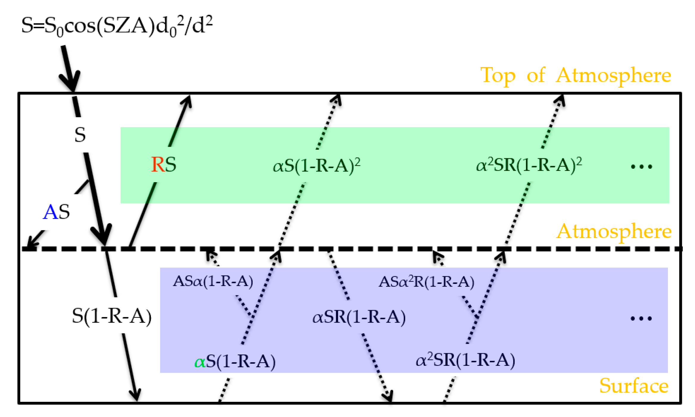
The theoretical background of RSR is shown in Figure 1. In this figure, the solid line is the primary absorption and reflection path of the shortwave radiation (extraterrestrial solar irradiation) incident on the atmosphere, and the dotted line shows the multiple scattering process by the surface and atmosphere [33]. RSR is green-shadowed in this schematic. It was approximated by using an infinite geometric series, as shown in Equation (1), because atmospheric reflection (R) times surface albedo (α) is less than 1 (αR < 1) [34]. In Equation (1), the solar constant (=1361 Wm−2) [35] and the SZA [36] are calculated by the theoretical equation in the previous study, however, TOA albedo can be retrieved using the narrowband reflectance of each CH and regression coefficients, as expressed by Equation (2) [11,13,14,15].
In Equations (1) and (2), A, R, and α are atmospheric absorption, scattering, and surface albedo, respectively; S0, and d02/d2 are solar constant, and earth-to-sun distance in astronomical units; c1–6 is the regression coefficient according to geometry of the solar-viewing and atmospheric conditions; and , , , , , and are the narrowband reflectance of each CH.
3.2. Reflected Shortwave Radiation Retrieval Algorithm
The step-by-step algorithm is shown in Figure 2. As shown in this figure, Himawari-8/AHI was converted into reflectance for each CH using radiance (Process 1). As shown in Equation (2), TOA albedo was retrieved by the narrowband reflectance and the regression coefficient LUT according to geometry of the solar-viewing and atmospheric conditions. Finally, SG was removed and RSR was retrieved using Equation (1). The regression coefficient used in this study was simulated, as shown in Table 2, using the SBDART according to the geometry of the solar-viewing and atmospheric conditions. More specifically, the SBDART simulation was performed under the following conditions: 12 SZAs, 18 VZAs, 19 RAAs, six atmospheric profiles, and five surface types in the 3.3 µm range at 0.2. Additionally, four aerosol types and four aerosol visibilities in the clear-sky area, and eight cloud heights and five cloud optical thicknesses in the cloud-area were included when configuring the simulation conditions. The regression coefficients can be obtained with a multiple linear regression model or ridge regression model, based on the simulation results (independent variables: reflectance of each CH taking into account anisotropy; dependent variable: TOA albedo). When a multiple linear regression model is used to determine the regression coefficient with the least square method [11,13], multicollinearity arises because of the high correlations between the shortwave CHs [37,38], thus lowering the accuracy of the regression coefficient; therefore, we used a ridge regression model [39,40]. Lee et al. [23] compared the accuracy of TOA albedos estimated by a multiple linear regression model and a ridge regression model with the Himawari-8/AHI data of 20 August 2015, by checking their respective results against the corresponding CERES data. The comparison revealed that the ridge regression model outperformed the multiple linear regression model in terms of R2 and RMSE (0.914 and 0.055 vs. 0.856 and 0.191).
3.2.1. Anisotropy Consideration
The TOA albedo retrieved by previous studies [23] was calculated assuming the narrowband reflectance to be isotropic. However, in this study, RSR was retrieved considering anisotropy. In other words, in Lee et al.’s [23] algorithm, the radiance of each CH was converted into the reflectance of each CH. As in Equation (2), the regression coefficient LUT were produced according to geometry of the solar-viewing and atmospheric conditions to retrieve the TOA albedo. The regression coefficients used in their study were based on the results of numerical experiments using the SBDART, in which simulations were performed according to atmospheric conditions, and a ridge regression (independent variables: narrowband reflectance of each CH assuming isotropy as in Equation (3); dependent variables: TOA albedo integrated from 0.2 to 3.3 µm using SBDART). In this process, the narrowband reflectance of each CH is assumed to be isotropic as shown in Equation (3). However, to retrieve TOA albedo accurately, the narrowband reflectance should be expressed as anisotropy, as shown in Equations (4) and (5). The anisotropy of the reflectance for each CH varies depending on the atmospheric conditions (surface type, absence/presence of clouds, etc.) [17,41,42,43,44]. Moreover, in the process of converting radiance into irradiance using Equation (3), the error in the mean dispersion was found to be higher when the Lambertian assumption (i.e., no anisotropic correction) was adopted than when anisotropy was considered (16.9% vs. 2.2%) [45].
In Equations (3)–(5), Li and S0,i are the radiance at the top of the atmosphere and the solar constant of each CH, respectively; SAA, and VAA are solar azimuth angle, and viewing azimuth angle, respectively; and Fi and ADM are irradiance at the top of the atmosphere of each CH [46] and anisotropy [16], respectively.
Considering the abovementioned factors, in this study, the regression coefficient LUT and the TOA albedo were calculated by considering the anisotropy of reflectance for each CH, as shown in Equations (4) and (5). The results were compared with those of Lee et al. [23]. Himawari-8/AHI, Terra, Aqua, and S-NPP/CERES data on the 15th day of each month from July 2015 to February 2017 (all 60 cases) were used. TOA albedo considering isotropy and anisotropy using narrowband reflectance is shown in Table 2.
3.2.2. Sun Glint Removal
SG is a phenomenon in which sunlight reflected from the Earth’s surface is incident on the field of view of the satellite sensor depending on the geometry of the solar–viewing. The measured value becomes greater than the originally measured value, and therefore the reflection appears brighter [47]. Previous studies have reported that SG removal or correction is necessary because it can cause serious errors in ocean-related satellite output [48]. In this study, SG was calculated using information of the SZA, VZA, and RAA (Equation (6)), and statistical analysis was performed using Himawari-8/AHI and Terra/CERES data for proper SG removal (Figure 3 and Figure 4).
4. Results
4.1. Evaluation of the Reflected Shortwave Radiation Algorithm
4.1.1. Anisotropy Consideration
Table 3 compares the results of isotropic and anisotropic assumptions using Himawari-8/AHI and the TOA albedo of Terra, Aqua, and S-NPP/CERES for this study. R2 values between isotropic and anisotropic Terra, Aqua, and S-NPP/CERES were similar. However, relative Bias (%Bias) and relative RMSE (%RMSE) were −1.14% and 21.04%, respectively, for anisotropic cases, which were improved from the isotropic case (%Bias = 5.16%; %RMSE = 22.67%), and the mean percentage error (MPE) was also improved. The cases of 15 July 2015, 15 May 2016, 15 June 2016, and 15 July 2016 showed better isotropy than the anisotropy, and the cause will be further discussed in Figure 6.
4.1.2. Sun Glint Removal
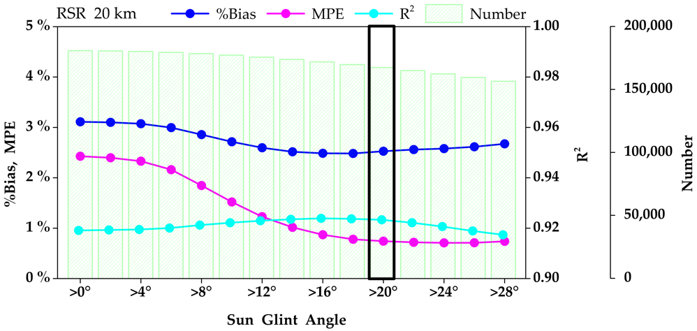
Because RSR significantly varies from clear skies to deep convective clouds (0 to 80%) [18], the case of 15 October 2015 was selected, with the accompanying precipitation and typhoons (KOPPU: 16.0°N, 138.8°E, and CHAMPI: 13.3°N, 158.2°E). Figure 3 shows the result of statistical analysis of R2, %Bias and MPE according to SG as an example of 15 October 2015 for the calculation of a proper angle for SG removal. As shown in this figure, R2 between Himawari-8/AHI and Terra/CERES was changed from 0.919 to 0.923 and %Bias from 3.11% to 2.53%. The MPE of Himawari-8/AHI and Terra/CERES decreased with increasing sun reflection angle, which was less than 0.74% when the SG was 20°. In this study, sun reflection angles less than 20° were considered as SG.
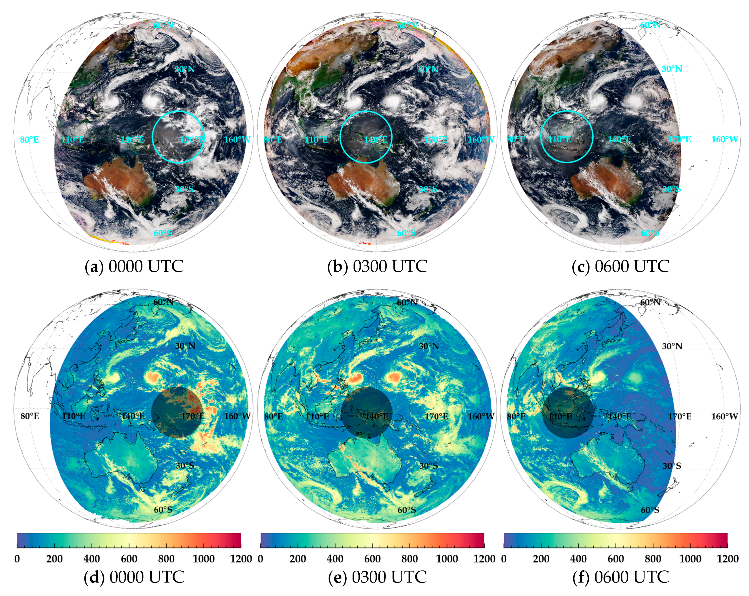
Figure 4 shows Red–Green–Blue (Blue: CH1, Green: CH2, Red: CH3, RGB) composite images (Figure 4a–c) and RSR (Figure 4d–f) of Himawari-8/AHI analyzing scene error according to SG. In this figure, the black circles (transparency = 50%) represent SG areas (≤20°). Figure 4g–j shows the RSR, percentage error, and SG of Himawari-8/AHI and Terra/CERES, respectively, with space-time agreement. In the RGB composite images in Figure 4a–c, SG appears brighter than the surrounding pixels of the mid-latitude ocean. This corresponds to the RSR pictures in Figure 4d–f. The MPE of Himawari-8/AHI and Terra/CERES was more than 45% (Figure 4i) and the SG angle was less than 20° (Figure 4j). In other words, when the SG area is removed, R2 between AHI and CERES is 0.919, which is larger than 0.923, and this result is consistent with the result of [17].
4.1.3. Reflected Shortwave Radiation
Lee et al. [23] retrieved TOA albedo assuming narrowband reflectance to be isotropic. In this study, RSR was retrieved by considering anisotropy of the narrowband reflectance by the surface and the atmosphere, and by removing SG. The results are shown in Figure 5. This figure shows the results of RSR of this study. Isotropic, anisotropic, and SG effects of narrowband reflectance were analyzed using the Himawari-8/AHI data (all data: 3,411,624 pixels). Figure 5a is a two-dimensional histogram (2D histogram) of the Terra/CERES data, with RSR retrieved assuming the narrowband reflectance to be isotropic Lee et al. [23] (OLD). Figure 5b,c shows the RSR considering anisotropy of the narrowband reflectance (OLD2)and the case of removing SG (OLD3), respectively. Figure 5d considers Figure 5b,c together; similar to Figure 5a, Figure 5b–d shows scatter plots along with Terra/CERES data. R2 between RSR retrieved using the Himawari-8/AHI and Terra/CERES data was 0.910 when the narrowband reflectance was assumed to be isotropic as shown in Figure 5a. The Bias and RMSE were 15.13 and 53.94 Wm−2, respectively. However, in this study, R2 between Himawari-8/AHI and Terra/CERES considering narrowband reflectance as anisotropy was 0.912, which is higher than that in Figure 5a. Furthermore, the Bias and RMSE were 2.80 and 50.14 Wm−2, respectively, showing improvements compared to Figure 5a. Comparing Figure 5a,c, R2 values are similar, but Bias and RMSE improved slightly. The narrowband reflectance was considered to be anisotropic and SG was removed simultaneously (NEW). Comparing Figure 5a,d, R2 (0.914), Bias (2.07 Wm−2) and RMSE (49.22 Wm−2) were significantly improved. These results are in good agreement with the results of [17], where R2 values between Meteosat RSR and ScaRaB RSR were found to be 0.845 and 0.863, respectively, for isotropic and anisotropic calculations.
4.2. Validation of Reflected Shortwave Radiation Algorithm Using CERES Data
The narrowband radiance of Himawari-8/AHI and the regression coefficient LUT were applied to the algorithm in Figure 2, and the RSR was retrieved and compared with Terra, Aqua, and S-NPP/CERES data (Figure 6). For validating the method, scalar accuracy measurement and linear relationship analysis were performed. For the scalar accuracy measurement, Bias, relative Bias (%Bias = Bias/CERESMea × 100%), root mean square error (RMSE), relative RMSE (%RMSE = RMSE/CERESMean × 100%) and mean percentage error (MPE = ((AHI-CERES)/CERES) × 100%) of Terra, Aqua, and S-NPP/CERES were calculated [49]. In addition, Pearson correlation coefficients [50] and significance level [51] were calculated through correlation analysis and Monte Carlo simulation to determine the linear relationship between the two data sets. For this purpose, SZA and VZAs less than 80° were used and SG angles less than 20° were excluded.
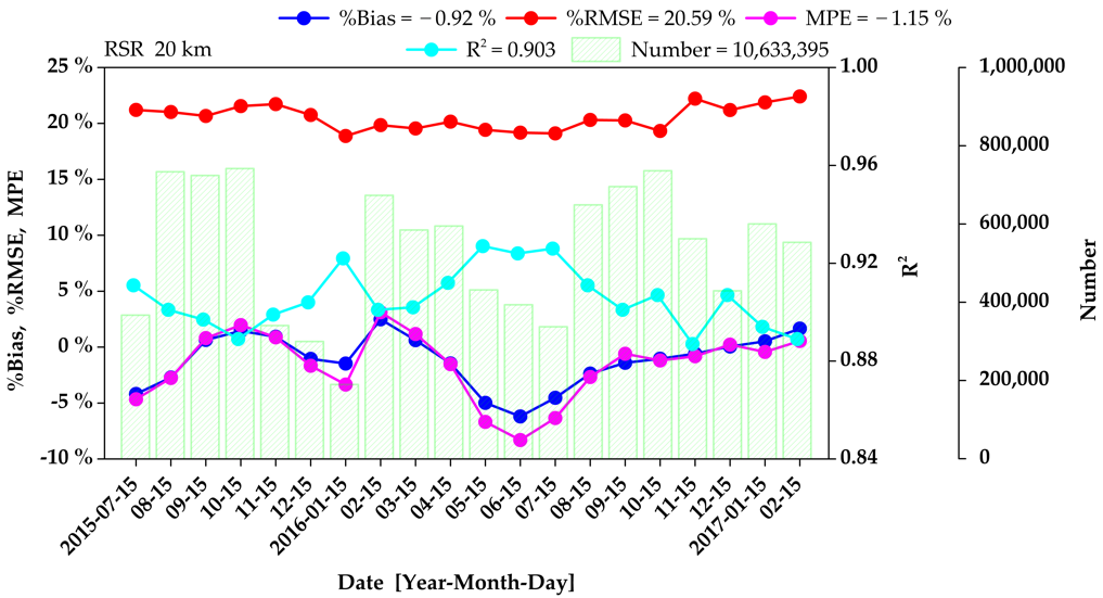
Figure 6 shows a comparison of Terra, Aqua, and S-NPP/CERES with RSR from Himawari-8/AHI. Excluding May–July 2016 cases, %Bias was −4.18–2.49% and MPE was −4.66–3.12%. Between May and July 2016, %Bias and MPE were much lower at −6.20 and −8.31%, respectively, on 15 June 2016, which is consistent with the results of TOA albedo statistical analysis in Table 3 (%Bias, MPE). To clarify the reason for such a result, clouds were subdivided according to the clear fraction (0–100%) used for the RSR retrieval. At this time, overcast was classified as 0–5%, mostly cloudy 5–50%, partly cloudy 50–95%, and clear 95–100% [46].
Figure 7 shows Bias, standard deviation (Stdev), RMSE, and R2 according to the clear fraction, and the bar chart means the number of data. Except for clear (95–100%) and cloudy fractions (0–5%), R2 (0.571–0.815) and RMSE (25.09–64.61 Wm−2) of Terra, Aqua, and S-NPP/CERES were not suitable for partly cloudy and mostly cloudy fractions (5–95%). The reason is that averaging the RSR of AHI in the process of spatial resolution matching can generate large errors when the averaged area characteristics (surface or cloud) are different from the CERES observations [20]. In particular, these errors were large in the cloudy area. The number of data in clear area (95–100%)/cloudy area (0–95%) was compared with the all data in each case. On 15 June 2016, the value was 5.94%/94.06% and, compared to other cases (8.71–14.15%/85.85–91.29%), there were less clear areas and too much cloud. Therefore, the results of this study and CERES statistical analysis were unsatisfactory. In the case of RSR retrieval, for error analysis in cloudy areas (<95%), Terra, Aqua, and S-NPP/CERES data were analyzed according to land, ocean, and clear fractions (partly cloudy, mostly cloudy, overcast, and all). Table 4 shows the results. For the ocean area, results of the statistical analysis (R2, Bias, MPE) were relatively better than that for the land, but both land and ocean area were partly or mostly cloudy, and this tendency was also consistent with MPE.
To analyze the detailed results according to the validation data of the Figure 6, the statistical analysis results of the three data sets (Terra, Aqua, and S-NPP) are shown in the Figure 8. Bias (%Bias), RMSE (%RMSE), and MPE were improved in the order of Terra, Aqua, and S-NPP. In the case of Terra, %Bias, %RMSE, and MPE were 0.83%, 19.82%, and 0.13%, respectively, while those for Aqua were −1.40%, 20.24%, and −1.59%, and −1.92%, 21.44%, and −1.85% for S-NPP. For further analysis of these results, the data for Terra, Aqua, and S-NPP were compared to those for the overall case according to the clear fraction (Figure 9). As shown in Figure 9, the number of data for clear areas in Terra was approximately 0.24% higher than that of Aqua and S-NPP but about 0.96%, 1.40%, and 1.89% less for cloudy areas (partly cloudy, mostly cloudy, and overcast). In the previous analysis, Terra’s error was smaller than that of Aqua and S-NPP because Terra had a slightly larger cloudy area and fewer clear areas than Aqua and S-NPP.
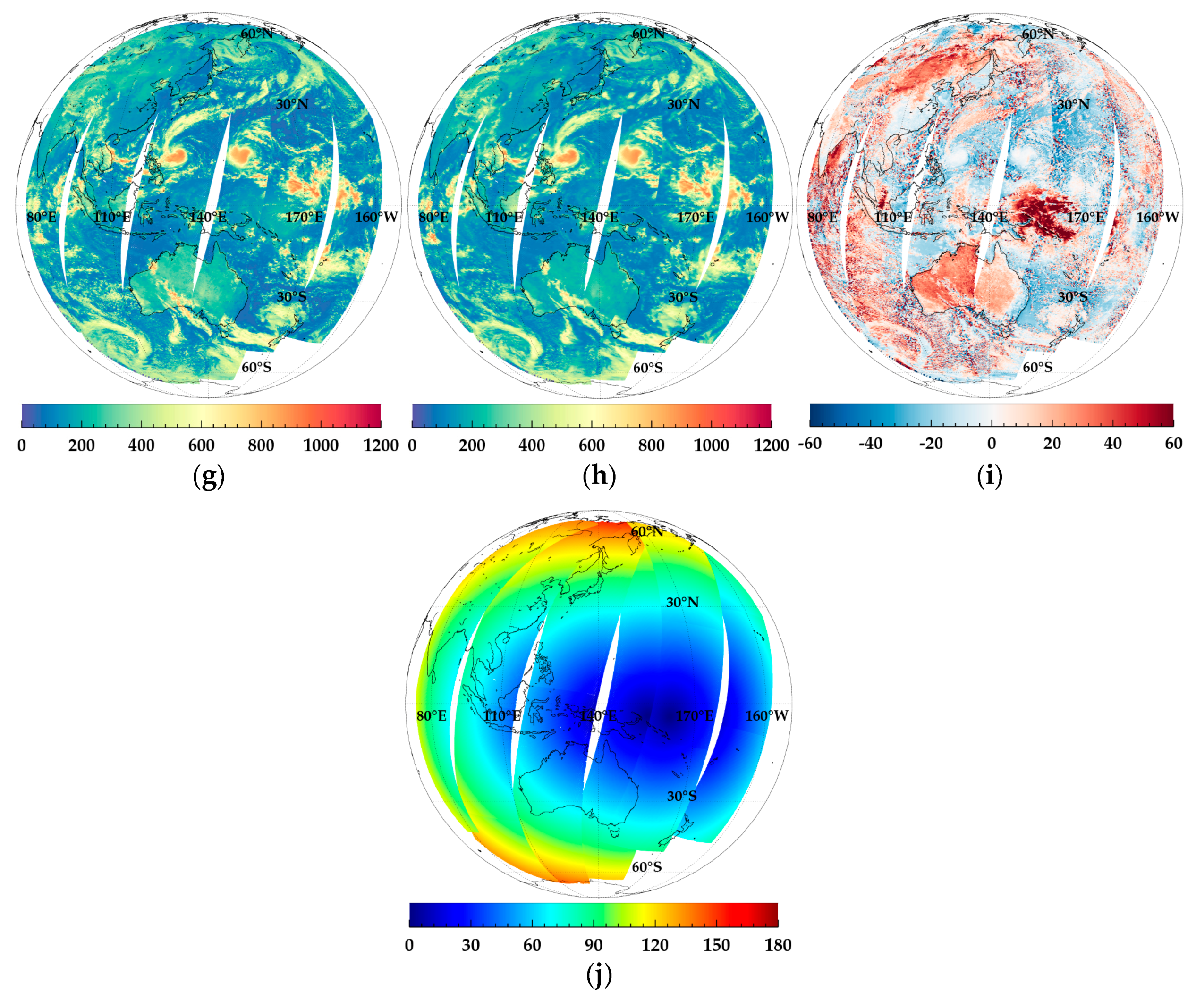
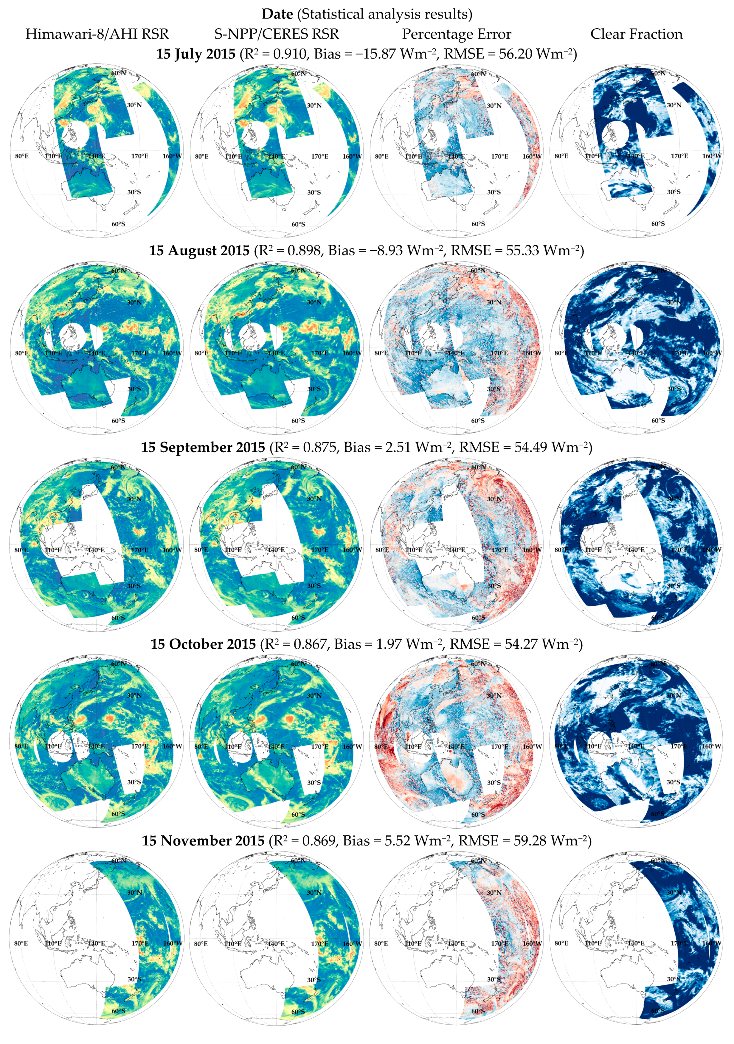
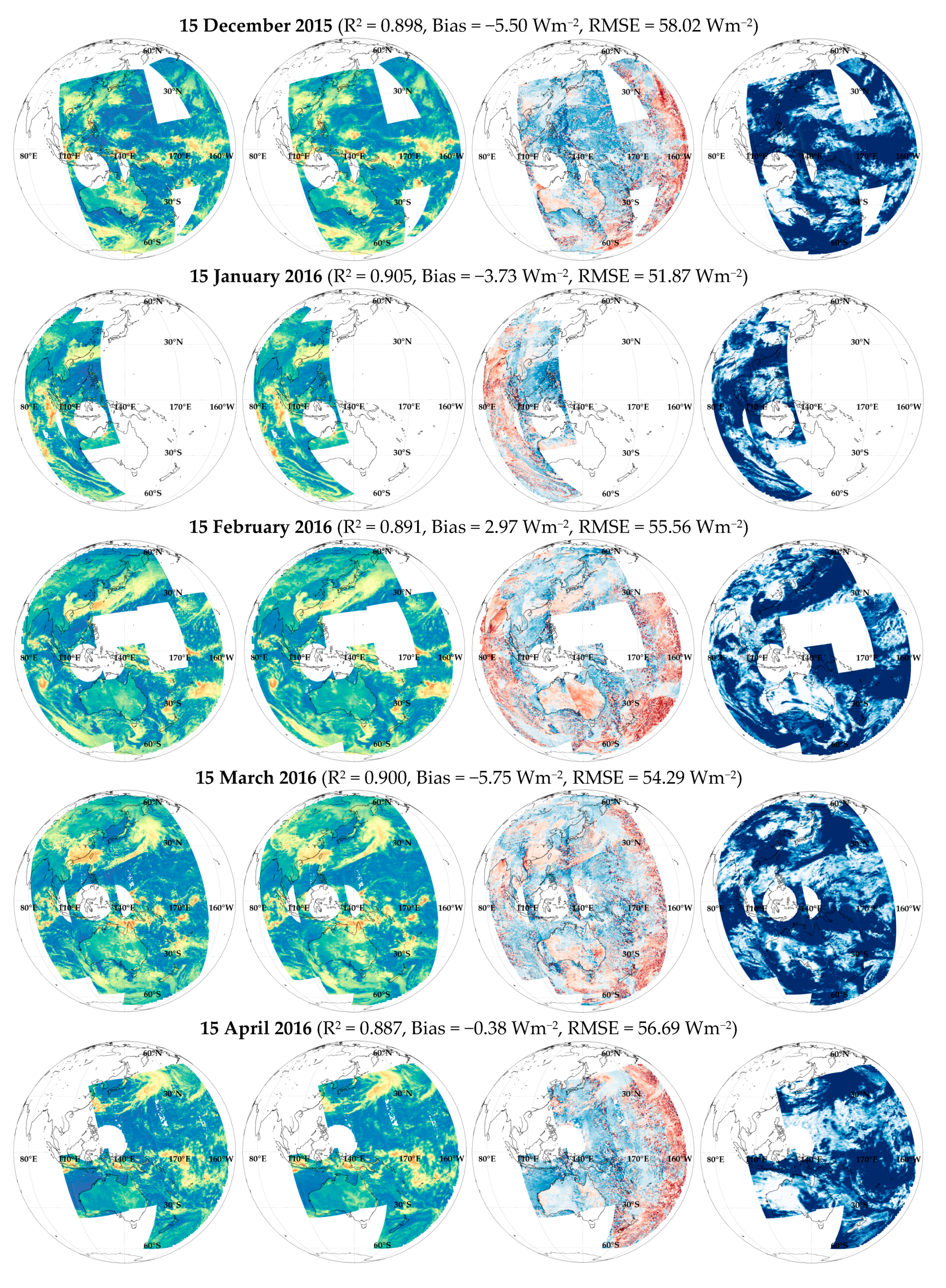
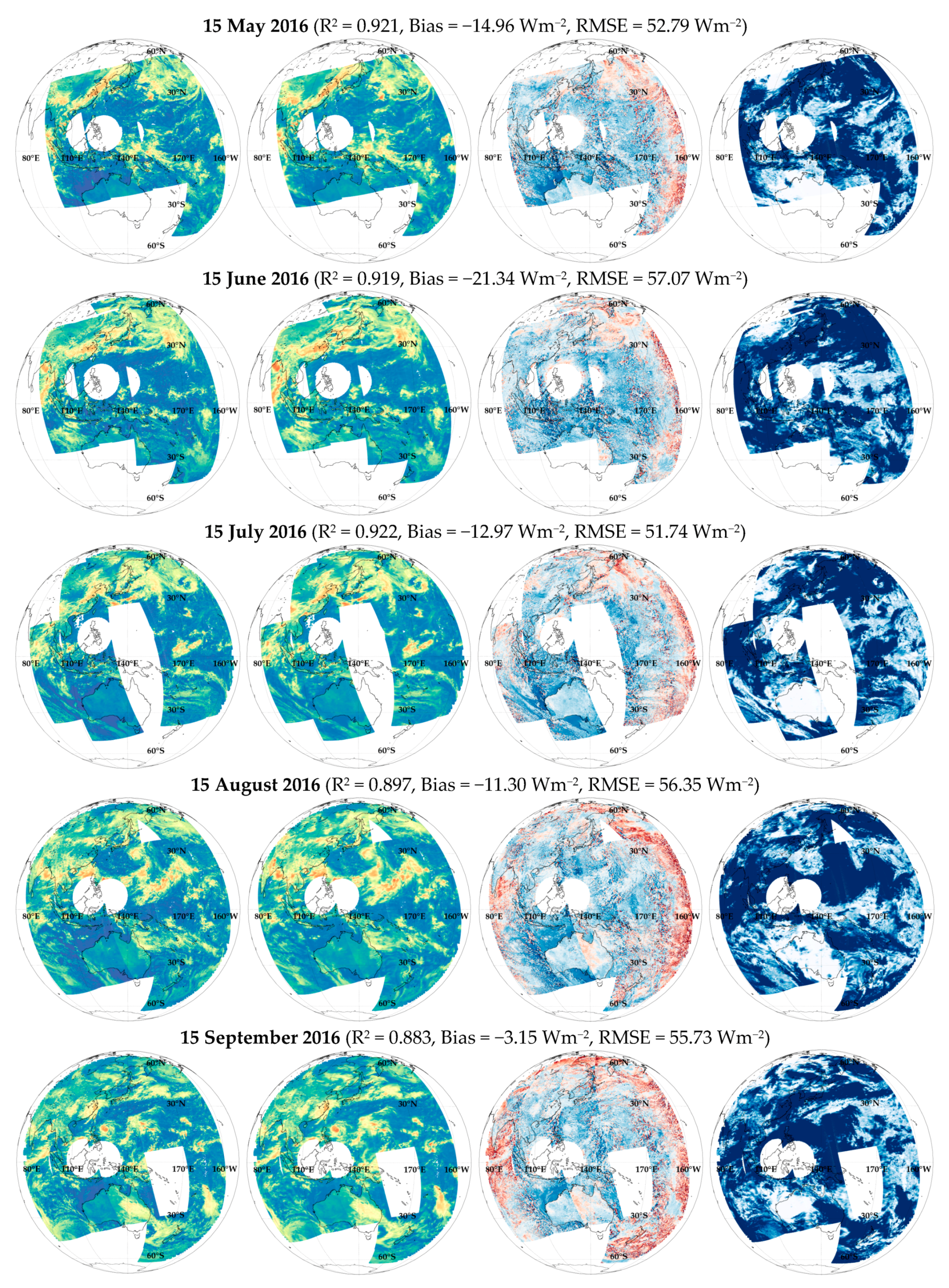
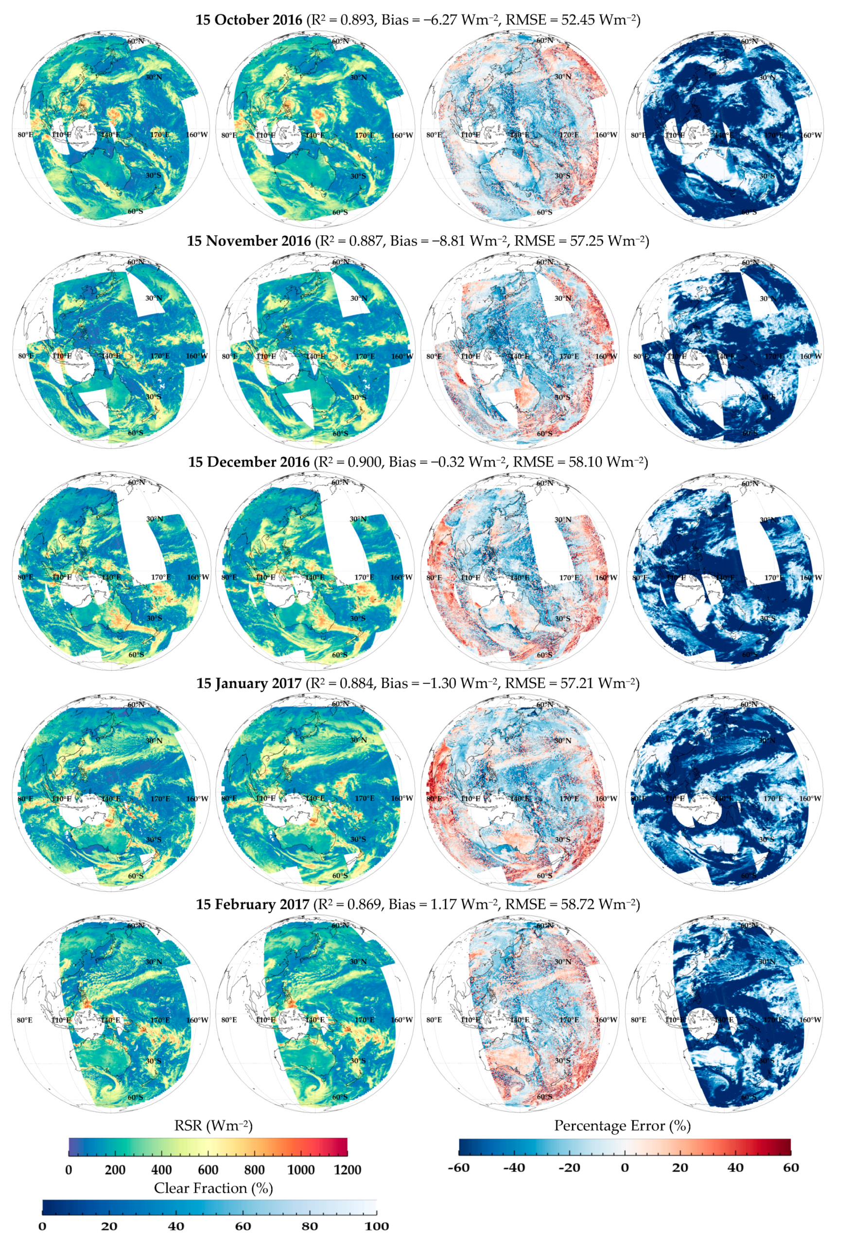
Figure 10 shows the results of scene analysis of S-NPP/CERES (36.08%) with the largest number of data among Terra, Aqua, and S-NPP for 20 cases because the S-NPP satellite observes at an altitude of 840 km, which is higher than the Terra and Aqua (705 km) [52]. Figure 10 shows the RSR of Himawari-8/AHI (left) and S-NPP/CERES (middle left), the percentage error of the two data sets (middle right), and the clear fraction of CERES (right). In this figure, RSR differs depending on the absence or presence of clouds and surface types, and the SZA increases as the latitude increases. We analyzed SZA and VZAs of less than 80° with approximately 3–5 scan line for each case. However, some cases had only 1–2 scan line due to the absence of Himawari-8/AHI data. In this figure, R2 and Bias between Himawari-8/AHI and S-NPP/CERES were 0.867–0.922, and −21.34–5.52 Wm−2, respectively, and the RMSE was 51.74–59.28 Wm−2, similar to the results of [18]. Regarding land surface albedo (0.12–0.36) for the clear area (95–100%), the RMSE of S-NPP/CERES was 14.33–41.65 Wm−2. This value is somewhat less accurate than that for the ocean (0.03–0.06, RMSE = 14.39–24.17 Wm−2), which was relatively small and constant. During the preparation of the regression coefficient LUT, surface was classified into five types (vegetation, desert, snow, ocean, and lake), whereas CERES data were classified into 20 types [46], leading to some inaccuracies. In addition, in the cloud area, the RMSE varied between 54.08 and 61.52 Wm−2, depending on the cloud properties (cloud optical thickness, cloud fraction, cloud type, etc.). Partly and mostly cloudy areas showed larger errors compared with overcast areas, particularly with increasing SZA and VZA. This can be attributed to the generation of the regression coefficient LUT using SBDART [11,53] and the actual atmospheric error assuming plane-parallel atmospheres [18]. In addition, the inability to refine the LUT according to the atmospheric conditions was considered to lead to an error; SZA (12 including 0°, 10°, 20°, 30°, 40°, 50°, 60°, 65°, 70°, 75°, 80°, and 85°), VZA (18 from 0–85° at 5° intervals), and RAA (19 from 0–180° at 10° intervals) [53]. Vermote and kotchenova [54] reported an error of 0.002 for 22 SZA and VZAs and 73 RAAs.
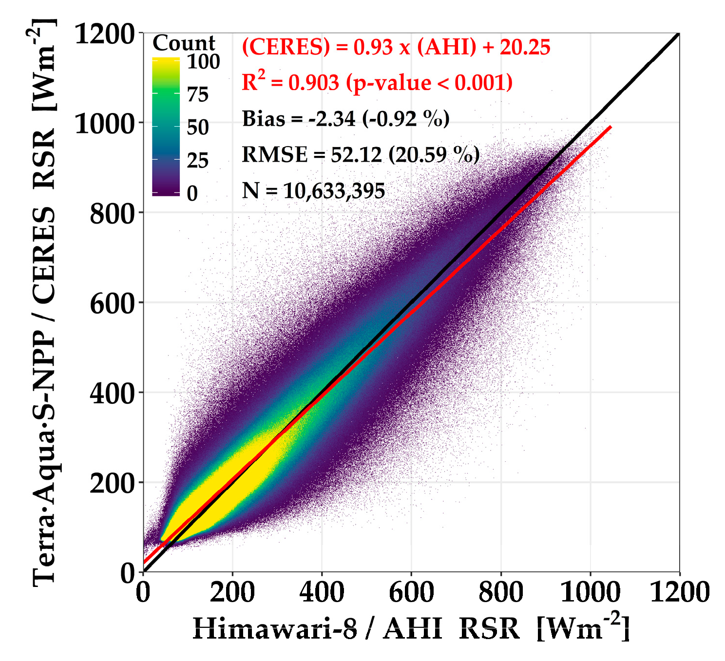
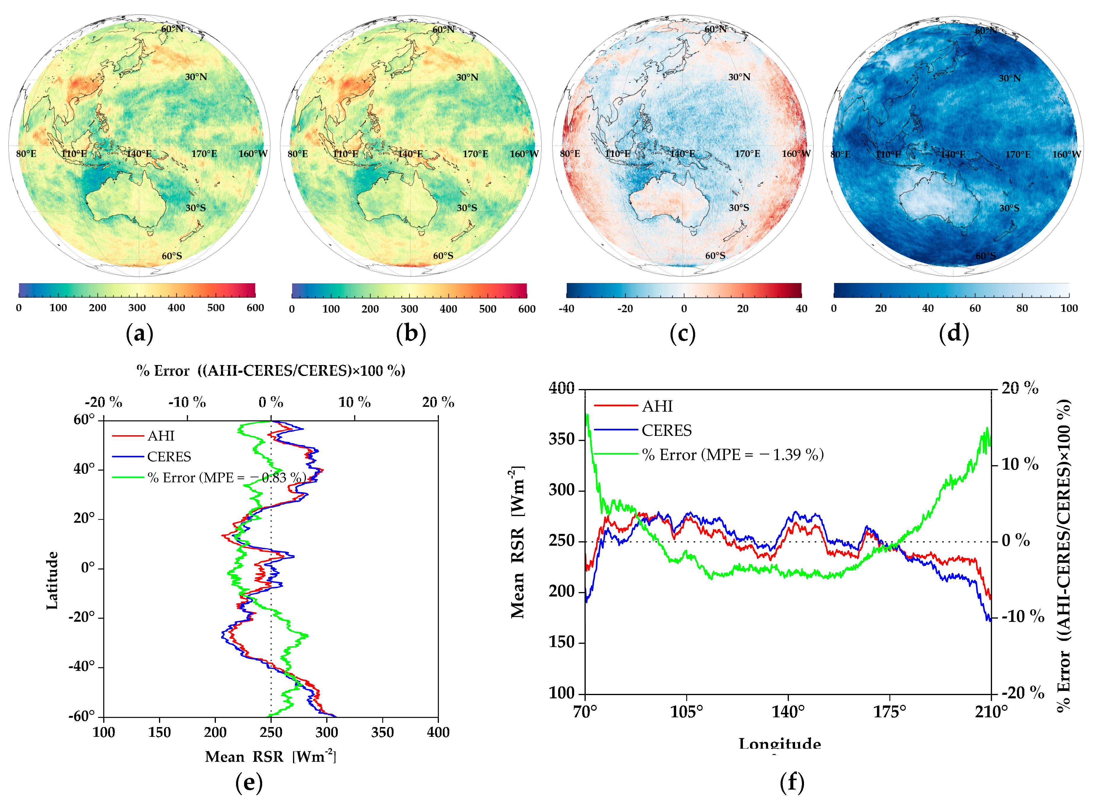
Figure 11 shows the results of averaging the data of Terra, Aqua, and S-NPP in the same manner averaging the RSR retrieved for these 20 cases with a resolution of 20 km for CERES. Figure 11 shows the averaged RSR (20 km) of AHI (Figure 11a) and CERES (Figure 11b) from 15 July 2015 to 15 February 2017, and the percentage error (Figure 11c) and the clear fraction (Figure 11d) of the two data sets. Figure 11e,f shows averaged results with respect to latitude and longitude, and RSR of AHI and CERES and the percentage error of both data sets, respectively. The results of this study, as shown in Figure 11a, are similar to the CERES average, as shown in Figure 11b. However, as shown in Figure 11c, the SZA and VZAs increases as sunrise or sunset approaches. In Figure 11e, the error between AHI and CERES for the latitude averages were within ±4%. However, the average longitude of Figure 11f had larger inaccuracies as bifurcations increased to 95 and 180° based on 140°. Then, in Figure 11d, the RSR of CERES above the Australian desert area shows a lower value than that of the AHI. This may be explained by the fact that RSR is greatly reduced by vapors, although the effects can vary in clear-sky areas depending on the surface type and absorption gases [55]. Since the CERES observes in the broadband shortwave range, RSR is greatly reduced in the range sensitive to vapor absorption (0.89–0.97 µm), whereas less attenuation occurs in the shortwave CHs of the Himawari-8/AHI used in this study because they are relatively transparent, compared to CERES. Similarly, the total precipitable water observed in this area during the study period was approximately 2.00 cm, indicating a MPE of approximately 3.81% in comparison to CERES. Therefore, the attenuation effect of vapors must be considered when retrieving RSR using a narrowband sensor. Figure 12 shows the results of this study (AHI) and Terra, Aqua, and S-NPP/CERES from 60 studies. In this figure, R2 is 0.903 and Bias and RMSE are −2.34 and 52.12 Wm−2, respectively.
5. Discussion
In this study, the narrowband reflectance that had been assumed to be isotropic in Lee et al. [23] was considered to be anisotropic and the RSR was retrieved by removing the sun reflection region that caused a large error. Because the anisotropy of the atmosphere differs depending on the geometry of the solar-viewing, as well as the characteristics of the Earth’s surface, the results improved in comparison with the CERES data when anisotropy was considered; the errors are listed in Table 3. Furthermore, SG below 20° was removed through statistical analysis (Figure 3) because strong sun reflection appears in a specific direction compared to the theoretical value and causes large errors in ocean areas [47,56]. After the SG was removed, the R2 between the AHI and CERES was 0.923, which is higher than the value when SG was not removed (R2 = 0.919). Furthermore, the Bias and MPE decreased from 3.11% and 2.43% to 2.53% and 0.74%, respectively. Based on these results, either the narrowband reflectance was assumed to be anisotropic or the SG was removed, as shown in Figure 5. The case where the narrowband reflectance was considered to be anisotropic and the SG was removed showed better results than the other cases, i.e., the case where the narrowband reflectance was assumed to be isotropic or considered anisotropic, or SG removed. In other words, consideration of anisotropy and removal of SG at the time of retrieving the RSR can reduce the error, as suggested by [17].
We compared the RSR retrieved using Himawari-8/AHI with the RSR observed in Terra, Aqua, and S-NPP/CERES. In this process, errors were generated by differences in spatial resolution and discrepancies in observation time (validation of ±5 min data, i.e., 0010 UTC vs. 0005‒0015 UTC) between AHI (2 km) and CERES (20 km) (Figure 7). To solve this problem, it is desirable to select and analyze a spatiotemporal resolution that shows good results by performing statistical analysis according to spatial resolution (0.5°, 1°, 2°, 5°, and 10°) for each daily or monthly average, as suggested by [2]. In addition, instead of analyzing data from only one satellite, all the Terra, Aqua and S-NPP data should be used together to carry out relatively continuous validation because polar-orbiting satellites equipped with broadband sensors perform observations only for specific time periods. Furthermore, when all the 60 cases and satellite data used in this study were averaged, relatively large errors were generated at SZA and VZAs above 70°, as shown in Figure 11. This is because several satellite-based data are error-prone due to the lack of accuracy in sunrise and sunset times [57]. Furthermore, the refraction effect at a SZA of 85° or less is negligible between the apparent SZA and the real SZA but produces significant errors at sunrise or sunset [58].
Even though errors were due to the difference between the spatiotemporal resolution and the SZA and VZAs, the validation results in Figure 12 show a similar trend to results presented in [1,18]. However, since the spatial resolution of the averaged satellite data was greater and more long-term analysis was performed in the current study, the R2 [59], Bias and RMSE [2,60] all improved. Therefore, the results of this study are improved in comparison to those of other studies [2,12,60].
6. Conclusions
This study used Himawari-8/AHI data to develop an algorithm for retrieving RSR. Himawari-8/AHI data have characteristics similar to those of the next-generation geostationary orbit meteorological satellite (GK-2A/AMI), which is to be launched in 2018. This algorithm converts the radiance of narrowband sensor into reflectance and then into TOA albedo through a regression coefficient LUT according to geometry of the solar-viewing (SZA, VZA, and RAA) and atmospheric conditions (surface type and absence/presence of clouds). The regression coefficients used in this study were calculated through numerical experimental using the SBDART and ridge regression for the TOA albedo and narrowband reflectance of sensor channels considering anisotropy. In addition, statistical analysis was performed to remove SG because SG can cause serious errors. For this purpose, reflection angles less than 20° were removed. Terra, Aqua, and S-NPP/CERES data were used to validate this RSR.
The results of this study (Himawari-8/AHI) showed improved performance of the algorithm, and the validation with Terra, Aqua, and S-NPP/CERES data also showed good results, except from 15 May to 15 July 2016. In particular, on 15 June 2016, comparing all data, the number of data in the clear areas and the cloudy area was influenced, and therefore the statistical analysis results were unsatisfactory. R2 (0.571–0.815) and RMSE (25.09–64.61 Wm−2) of the partly and mostly cloudy areas were large, which could be attributed to a space-time mismatch between AHI and CERES in the spatial resolution matching process. To further analyze these results, we divided the data into three sets (Terra, Aqua, and S-NPP). The results were better in the order of Terra, Aqua, and S-NPP, because Terra accounted for a larger number of data in the clear area and less cloud area than Aqua and S-NPP. This implies that the validation results are affected by the number of data in the clear and cloudy areas.
The analysis of the scan line showed an RMSE of 14.33–41.65 Wm−2 on the land for the clear area, which slightly differs from that of the ocean (RMSE = 14.39–24.17 Wm−2) due to the classification difference of the surface type of AHI and CERES. In addition, because SBDART assumes a plane-parallel atmosphere in the cloud region, the error increases as the SZA and VZAs increase in the real atmosphere and the plane-parallel atmosphere. Nevertheless, R2 in this study was higher than 0.867 and Bias and RMSE were −21.34–5.52 and 51.74–59.28 Wm−2 for scan line, respectively. R2 between AHI and Terra, Aqua, and S-NPP/CERES for all case was 0.903, showing significance of approximately 0.001, and Bias and RMSE were −2.34 and 52.12 Wm−2, respectively.
High temporal and spatial resolution data, such as the next-generation geostationary meteorological satellites (Himawari-8/AHI, GK-2A/AMI, etc.), are used to conduct research on understanding the effects of aerosols [61] and clouds [62], which have large temporal and spatial variabilities, on radiation [18]. It can also be applied as basic input for numerical prediction and climate models, which will contribute to improving the accuracy of the calculation [63] and further monitoring of radiation balance to understand the mechanism of climate change [64]. As a preliminary study for the radiative element output of GK-2A/AMI, the successor satellite of the Republic of Korea, this study will guide future research and development of the sensor. Nevertheless, the algorithm cannot classify surface types [65] in clear areas and the RSR error is generated because cloudy areas do not reflect cloud properties (cloud optical thickness, cloud fraction, cloud type, etc.) in detail. Future studies will require a recalculation LUT that reflects the characteristics of the surface and clouds and should be periodically corrected by long-term observed broadband radiation [5,66].
Acknowledgments
This work was supported by “Development of Radiation/Aerosol Algorithms” project, funded by ETRI, which is a subproject of “Development of Geostationary Meteorological Satellite Ground Segment (NMSC-2016-01)” program funded by NMSC (National Meteorological Satellite Center) of KMA (Korea Meteorological Administration).
Author Contributions
Sang-Ho Lee led manuscript writing and contributed to the data analysis and research design. Kyu-Tae Lee and Bu-Yo Kim supervised this study, contributed to the research design and manuscript writing, and served as the corresponding authors. Il-Sung Zo, Hyun-Seok Jung and Se-Hun Rim contributed to the discussion of the results and manuscript writing.
Conflicts of Interest
The authors declare no conflict of interest.
References
- AWG Radiation Budget Application Team. GOES-R Advanced Baseline Imager (ABI) Algorithm Theoretical Basis Document for Downward Shortwave Radiation (Surface), and Reflected Shortwave Radiation (TOA), NOAA NESDIS Center for Satellite Applications and Research, 27 September 2010. Available online: https://www.goes-r.gov/products/ATBDs/baseline/baseline-DSR-v2.0.pdf (accessed on 28 November 2017).
- Bhartia, P.K. Top-of-the-atmosphere shortwave flux estimation from satellite observations: An empirical neural network approach applied with data from the a-train constellation. Atmos. Meas. Tech. 2016, 9, 2813–2826. [Google Scholar]
- Kim, Y.-J.; Kim, B.-G.; Miller, M.; Min, Q.; Song, C.-K. Enhanced aerosol-cloud relationships in more stable and adiabatic clouds. Asia-Pac. J. Atmos. Sci. 2012, 48, 283–293. [Google Scholar] [CrossRef]
- Trenberth, K.E.; Dai, A.; Van Der Schrier, G.; Jones, P.D.; Barichivich, J.; Briffa, K.R.; Sheffield, J. Global warming and changes in drought. Nat. Clim. Chang. 2014, 4, 17–22. [Google Scholar] [CrossRef]
- Doelling, D.R.; Loeb, N.G.; Keyes, D.F.; Nordeen, M.L.; Morstad, D.; Nguyen, C.; Wielicki, B.A.; Young, D.F.; Sun, M. Geostationary enhanced temporal interpolation for CERES flux products. J. Atmos. Ocean. Technol. 2013, 30, 1072–1090. [Google Scholar] [CrossRef]
- Stephens, G.L.; O’Brien, D.; Webster, P.J.; Pilewski, P.; Kato, S.; Li, J.L. The albedo of earth. Rev. Geophys. 2015, 53, 141–163. [Google Scholar] [CrossRef]
- Hatzianastassiou, N.; Matsoukas, C.; Fotiadi, A.; Pavlakis, K.; Drakakis, E.; Hatzidimitriou, D.; Vardavas, I. Global distribution of earth’s surface shortwave radiation budget. Atmos. Chem. Phys. 2005, 5, 2847–2867. [Google Scholar] [CrossRef]
- Stubenrauch, C.; Rossow, W.; Kinne, S. Assessment of global cloud data sets from satellites a project of the world climate research programme global energy and water cycle experiment (GEWEX) radiation panel lead authors. Am. Meteorol. Soc. 2012. [Google Scholar] [CrossRef]
- Luther, M.; Cooper, J.; Taylor, G. The earth radiation budget experiment nonscanner instrument. Rev. Geophys. 1986, 24, 391–399. [Google Scholar] [CrossRef]
- Wielicki, B.A.; Barkstrom, B.R.; Harrison, E.F.; Lee, R.B., III; Louis Smith, G.; Cooper, J.E. Clouds and the earth’s radiant energy system (CERES): An earth observing system experiment. Bull. Am. Meteorol. Soc. 1996, 77, 853–868. [Google Scholar] [CrossRef]
- Wang, D.; Liang, S. Estimating high-resolution top of atmosphere albedo from moderate resolution imaging spectroradiometer data. Remote Sens. Environ. 2016, 178, 93–103. [Google Scholar] [CrossRef]
- Niu, X.; Pinker, R.T. Revisiting satellite radiative flux computations at the top of the atmosphere. Int. J. Remote Sens. 2012, 33, 1383–1399. [Google Scholar] [CrossRef]
- Buriez, J.C.; Parol, F.; Poussi, Z.; Viollier, M. An improved derivation of the top-of-atmosphere albedo from POLDER/ADEOS-2: 2. Broadband albedo. J. Geophys. Res. Atmos. 2007, 112. [Google Scholar] [CrossRef]
- Laszlo, I.; Gruber, A.; Jacobowitz, H. The relative merits of narrowband channels for estimating broadband albedos. J. Atmos. Ocean. Technol. 1988, 5, 757–773. [Google Scholar] [CrossRef]
- Wydick, J.E.; Davis, P.A.; Gruber, A. Estimation of Broadband Planetary Albedo from Operational Narrowband Satellite Measurements; National Oceanic and Atmospheric Administration: Washington, DC, USA, 1987.
- Loeb, N.G.; Manalo-Smith, N.; Kato, S.; Miller, W.F.; Gupta, S.K.; Minnis, P.; Wielicki, B.A. Angular distribution models for top-of-atmosphere radiative flux estimation from the clouds and the earth’s radiant energy system instrument on the tropical rainfall measuring mission satellite. Part I: Methodology. J. Appl. Meteorol. 2003, 42, 240–265. [Google Scholar] [CrossRef]
- Viollier, M. Restitution of longwave and shortwave radiative fluxes at the top of the atmosphere from combination of scarab and meteosat data. In Proceedings of the Megha-Tropiques 2nd Scientific Workshop, Paris, France, 2–6 July 2001. [Google Scholar]
- Vazquez-Navarro, M.; Mayer, B.; Mannstein, H. A fast method for the retrieval of integrated longwave and shortwave top-of-atmosphere upwelling irradiances from MSG/SEVIRI (RRUMS). Atmos. Meas. Tech. 2013, 6, 2627–2640. [Google Scholar] [CrossRef] [Green Version]
- Berk, A.; Bernstein, L.; Robertson, D. Modtran: A Moderate Resolution Model for LOWTRAN 7; Rep. AFGL-TR-83-0187; Air Force Geophysical Laboratory, Hanscom Air Force Base: Hanscom, MA, USA, 1983. [Google Scholar]
- Kim, B.-Y.; Lee, K.-T.; Jee, J.-B.; Zo, I.-S. Retrieval of outgoing longwave radiation at top-of-atmosphere using himawari-8 AHI data. Remote Sens. Environ. 2018, 204, 498–508. [Google Scholar] [CrossRef]
- Choi, Y.-S.; Ho, C.-H. Earth and environmental remote sensing community in South Korea: A review. Remote Sens. Appl. Soc. Environ. 2015, 2, 66–76. [Google Scholar] [CrossRef]
- Murata, H.; Takahashi, M.; Kosaka, Y. Vis and IR bands of Himawari-8/AHI compatible with those of MTSAT-2/Imager. 2015. Available online: www.data.jma.go.jp/mscweb/technotes/msctechrep60.pdf (accessed on 30 January 2018).
- Lee, S.-H.; Lee, K.-T.; Kim, B.-Y.; Zo, I.-S.; Jung, H.-S.; Rim, S.-H. Retrieval Algorithm for Broadband Albedo at the Top of the Atmosphere. Asia Pac. J. Atmos. Sci. 2017, accepted. [Google Scholar]
- Ricchiazzi, P.; Yang, S.; Gautier, C.; Sowle, D. Sbdart: A research and teaching software tool for plane-parallel radiative transfer in the earth’s atmosphere. Bull. Am. Meteorol. Soc. 1998, 79, 2101–2114. [Google Scholar] [CrossRef]
- Bessho, K.; Date, K.; Hayashi, M.; Ikeda, A.; Imai, T.; Inoue, H.; Kumagai, Y.; Miyakawa, T.; Murata, H.; Ohno, T. An introduction to himawari-8/9—Japan’s new-generation geostationary meteorological satellites. J. Meteorol. Soc. Jpn. Ser. II 2016, 94, 151–183. [Google Scholar] [CrossRef]
- Puschell, J.J.; Lowe, H.A.; Jeter, J.W.; Kus, S.M.; Hurt, W.T.; Gilman, D.; Rogers, D.L.; Hoelter, R.L.; Ravella, R. Japanese Advanced Meteorological Imager: A next-generation geo imager for MTSAT-1R. In Proceedings of the Earth Observing Systems VII, Seattle, WA, USA, 7–11 July 2002; International Society for Optics and Photonics: Bellingham, WA, USA, 2002; pp. 152–162. [Google Scholar]
- Cao, C.; De Luccia, F.J.; Xiong, X.; Wolfe, R.; Weng, F. Early on-orbit performance of the visible infrared imaging radiometer suite onboard the Suomi National Polar-Orbiting Partnership (S-NPP) satellite. IEEE Trans. Geosci. Remote Sens. 2014, 52, 1142–1156. [Google Scholar] [CrossRef]
- Yu, F.; Wu, X. Radiometric inter-calibration between Himawari-8 AHI and S-NPP VIIRS for the solar reflective bands. Remote Sens. 2016, 8, 165. [Google Scholar] [CrossRef]
- Paden, J.; Smith, G.L.; Lee, R.B.; Pandey, D.K.; Thomas, S. Reality check: A point response function (PRF) comparison of theory to measurements for the clouds and the earth’s radiant energy system (CERES) tropical rainfall measuring mission (TRMM) instrument. In Proceedings of the Visual Information Processing VI, Orlando, FL, USA, 21–25 April 1997; International Society for Optics and Photonics: Bellingham, WA, USA, 1997; pp. 109–118. [Google Scholar]
- Su, W.; Corbett, J.; Eitzen, Z.; Liang, L. Next-generation angular distribution models for top-of-atmosphere radiative flux calculation from CERES instruments: Validation. Atmos. Meas. Tech. 2015, 8, 3297–3313. [Google Scholar] [CrossRef]
- Zerefos, C.S.; Isaksen, I.S.; Ziomas, I. Chemistry and Radiation Changes in the Ozone Layer; Springer Science & Business Media: Berlin/Heidelberg, Germany, 2012; Volume 557. [Google Scholar]
- Blanc, P.; Gschwind, B.; Lefevre, M.; Wald, L. Twelve monthly maps of ground albedo parameters derived from MODIS data sets. In Proceedings of the IEEE International Geoscience and Remote Sensing Symposium (IGARSS), Quebec City, QC, Canada, 13–18 July 2014; pp. 3270–3272. [Google Scholar]
- Liang, S. Quantitative Remote Sensing of Land Surfaces; John Wiley & Sons: Hoboken, NJ, USA, 2005; Volume 30. [Google Scholar]
- Qu, X.; Hall, A. Surface contribution to planetary albedo variability in cryosphere regions. J. Clim. 2005, 18, 5239–5252. [Google Scholar] [CrossRef]
- Kopp, G.; Lean, J.L. A new, lower value of total solar irradiance: Evidence and climate significance. Geophys. Res. Lett. 2011, 38. [Google Scholar] [CrossRef]
- Michalsky, J.J. The astronomical almanac’s algorithm for approximate solar position (1950–2050). Sol. Energy 1988, 40, 227–235. [Google Scholar] [CrossRef]
- Nanni, M.R.; Demattê, J.A.M. Spectral reflectance methodology in comparison to traditional soil analysis. Soil Sci. Soc. Am. J. 2006, 70, 393–407. [Google Scholar] [CrossRef]
- Mokhtari, M.H.; Busu, I. Downscaling albedo from moderate-resolution imaging spectroradiometer (MODIS) to advanced space-borne thermal emission and reflection radiometer (ASTER) over an agricultural area utilizing aster visible-near infrared spectral bands. Int. J. Phys. Sci. 2011, 6, 5804–5821. [Google Scholar]
- Draper, N.R.; Smith, H.; Pownell, E. Applied Regression Analysis; Wiley: New York, NY, USA, 1966; Volume 3. [Google Scholar]
- Kleinbaum, D.; Kupper, L.; Nizam, A.; Rosenberg, E. Applied Regression Analysis and Other Multivariable Methods; Nelson Education: Scarborough, ON, Canada, 2013. [Google Scholar]
- Loeb, N.G.; Hinton, P.O.R.; Green, R.N. Top-of-atmosphere albedo estimation from angular distribution models: A comparison between two approaches. J. Geophys. Res. Atmos. 1999, 104, 31255–31260. [Google Scholar] [CrossRef]
- Loeb, N.G.; Parol, F.; Buriez, J.-C.; Vanbauce, C. Top-of-atmosphere albedo estimation from angular distribution models using scene identification from satellite cloud property retrievals. J. Clim. 2000, 13, 1269–1285. [Google Scholar] [CrossRef]
- Kato, S.; Marshak, A. Solar zenith and viewing geometry-dependent errors in satellite retrieved cloud optical thickness: Marine stratocumulus case. J. Geophys. Res. Atmos. 2009, 114. [Google Scholar] [CrossRef]
- Gardner, A.S.; Sharp, M.J. A review of snow and ice albedo and the development of a new physically based broadband albedo parameterization. J. Geophys. Res. Earth Surf. 2010, 115. [Google Scholar] [CrossRef]
- Loeb, N.G.; Kato, S. Top-of-atmosphere direct radiative effect of aerosols over the tropical oceans from the clouds and the earth’s radiant energy system (CERES) satellite instrument. J. Clim. 2002, 15, 1474–1484. [Google Scholar] [CrossRef]
- Geier, E.; Green, R.; Kratz, D.; Minnis, P.; Miller, W.; Nolan, S.; Franklin, C. Clouds and the Earth’s Radiant Energy System (CERES). Data Management System: Single Satellite Footprint TOA/Surface Fluxes and Clouds (SSF) Collection Document. Release 2 Version 1; 2003. Available online: https://ceres.larc.nasa.gov/documents/collect_guide/pdf/SSF_CG.pdf (accessed on 28 November 2017).
- Zhang, H.; Wang, M. Evaluation of sun glint models using MODIS measurements. J. Quant. Spectrosc. Radiat. Transf. 2010, 111, 492–506. [Google Scholar] [CrossRef]
- Kay, S.; Hedley, J.D.; Lavender, S. Sun glint correction of high and low spatial resolution images of aquatic scenes: A review of methods for visible and near-infrared wavelengths. Remote Sens. 2009, 1, 697–730. [Google Scholar] [CrossRef]
- Wilks, D.S. Statistical Methods in the Atmospheric Sciences; Academic Press: Cambridge, MA, USA, 2011; Volume 100. [Google Scholar]
- Benesty, J.; Chen, J.; Huang, Y.; Cohen, I. Pearson correlation coefficient. In Noise Reduction in Speech Processing; Springer: New York, NY, USA, 2009; pp. 1–4. [Google Scholar]
- Livezey, R.E.; Chen, W. Statistical field significance and its determination by Monte Carlo techniques. Mon. Weather Rev. 1983, 111, 46–59. [Google Scholar] [CrossRef]
- Thomas, S.; Priestley, K.; Shankar, M.; Smith, N.; Timcoe, M. Pre-launch sensor characterization of the CERES flight model 5 (FM5) instrument on NPP mission. Proc. SPIE 2011. [Google Scholar] [CrossRef]
- Lu, N.; Liu, R.; Liu, J.; Liang, S. An algorithm for estimating downward shortwave radiation from GMS 5 visible imagery and its evaluation over china. J. Geophys. Res. Atmos. 2010, 115. [Google Scholar] [CrossRef]
- Vermote, E.F.; Kotchenova, S. Atmospheric correction for the monitoring of land surfaces. J. Geophys. Res. Atmos. 2008, 113. [Google Scholar] [CrossRef]
- Sena, E.; Artaxo, P.; Correia, A. The effects of smoke aerosols, land-use change and water vapor reduction on the shortwave radiative budget over the Amazônia. In Proceedings of the EGU General Assembly Conference Abstracts, Vienna, Austria, 27 April–2 May 2014; Volume 16. [Google Scholar]
- Bertrand, C.; Clerbaux, N.; Ipe, A.; Dewitte, S.; Gonzalez, L. Angular distribution models anisotropic correction factors and sun glint: A sensitivity study. Int. J. Remote Sens. 2006, 27, 1741–1757. [Google Scholar] [CrossRef]
- Urraca, R.; Gracia-Amillo, A.M.; Koubli, E.; Huld, T.; Trentmann, J.; Riihelä, A.; Lindfors, A.V.; Palmer, D.; Gottschalg, R.; Antonanzas-Torres, F. Extensive validation of CM SAF surface radiation products over europe. Remote Sens. Environ. 2017, 199, 171–186. [Google Scholar] [CrossRef] [PubMed]
- Madhavan, B. Interactive comment on “shortwave surface radiation budget network for observing small-scale cloud inhomogeneity fields” by B.L. Madhavan et al. Atmos. Meas. Tech. Discuss. 2015, 8, C2233–C2250. [Google Scholar] [CrossRef]
- Li, Z.; Cribb, M.; Chang, F.L.; Trishchenko, A.; Luo, Y. Natural variability and sampling errors in solar radiation measurements for model validation over the atmospheric radiation measurement southern great plains region. J. Geophys. Res. Atmos. 2005, 110. [Google Scholar] [CrossRef]
- Wang, D.; Liang, S. Estimating top-of-atmosphere daily reflected shortwave radiation flux over land from modis data. IEEE Trans. Geosci. Remote Sens. 2017, 55, 4022–4031. [Google Scholar] [CrossRef]
- He, L.; Wang, L.; Lin, A.; Zhang, M.; Bilal, M.; Tao, M. Aerosol optical properties and associated direct radiative forcing over the Yangtze River basin during 2001–2015. Remote Sens. 2017, 9, 746. [Google Scholar] [CrossRef]
- Katagiri, S.; Kikuchi, N.; Nakajima, T.Y.; Higurashi, A.; Shimizu, A.; Matsui, I.; Hayasaka, T.; Sugimoto, N.; Takamura, T.; Nakajima, T. Cirrus cloud radiative forcing derived from synergetic use of MODIS analyses and ground-based observations. Sola 2010, 6, 25–28. [Google Scholar] [CrossRef]
- Allan, R.P.; Slingo, A.; Milton, S.F.; Culverwell, I. Exploitation of geostationary earth radiation budget data using simulations from a numerical weather prediction model: Methodology and data validation. J. Geophys. Res. Atmos. 2005, 110. [Google Scholar] [CrossRef]
- Urbain, M.; Clerbaux, N.; Ipe, A.; Tornow, F.; Hollmann, R.; Baudrez, E.; Velazquez Blazquez, A.; Moreels, J. The CM SAF TOA radiation data record using MVIRI and SEVIRI. Remote Sens. 2017, 9, 466. [Google Scholar] [CrossRef]
- Congalton, R.G.; Gu, J.; Yadav, K.; Thenkabail, P.; Ozdogan, M. Global land cover mapping: A review and uncertainty analysis. Remote Sens. 2014, 6, 12070–12093. [Google Scholar] [CrossRef]
- Doelling, D.R.; Sun, M.; Nguyen, L.T.; Nordeen, M.L.; Haney, C.O.; Keyes, D.F.; Mlynczak, P.E. Advances in geostationary-derived longwave fluxes for the CERES synoptic (SYN1deg) product. J. Atmos. Ocean. Technol. 2016, 33, 503–521. [Google Scholar] [CrossRef]
Figure 1.
Schematic representing the RSR (green area) in the one-layer solar radiation model. The line at the top of the atmosphere represents the atmospheric contribution (red) associated with cloud reflection, and the dotted line indicates the surface contribution (blue area) associated with surface reflection. The variables A, R, and α are atmospheric absorption and scattering of extraterrestrial solar irradiation, reflection by clouds, and surface albedo, respectively.

Figure 2.
Flow chart of the retrieval algorithm for RSR. Reflectance converted from radiance from each shortwave channel (CH) (Process 1) is used to retrieve RSR using regression coefficients look-up-table (LUT) according to geometry of the solar-viewing (SZA, VZA, and RAA) and atmospheric conditions (surface type and absence/presence of clouds) (Process 2). These regression coefficients were calculated using results from the radiative transfer model (SBDART), which considered geometry of the solar-viewing and atmospheric conditions, and a ridge regression model.
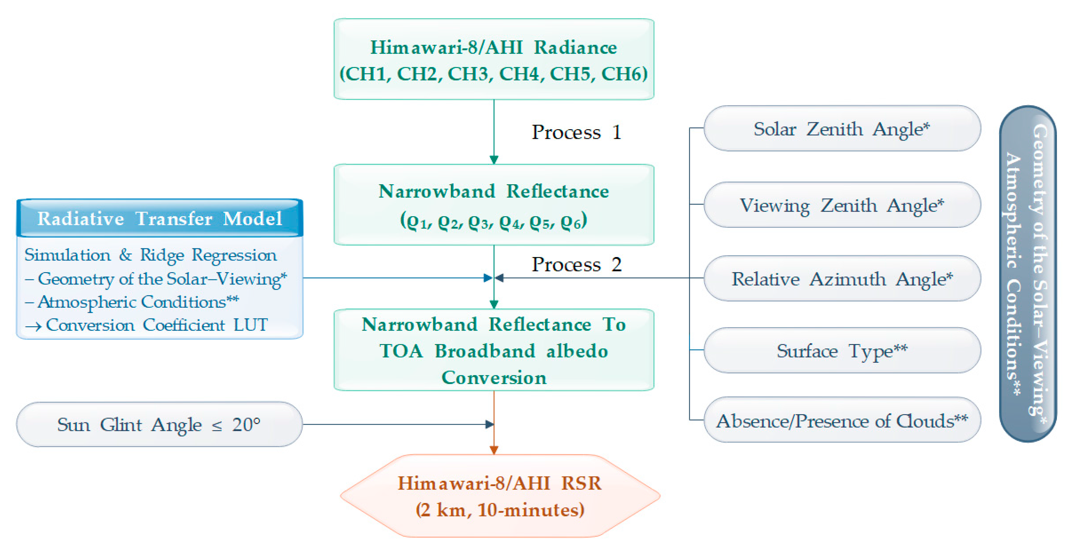
Figure 3.
Relative bias (%Bias), mean percentage error (MPE in percent), coefficient of determination (R2), and number in Himawari-8/AHI and Terra/CERES data sets as a function of sun glint (SG) angle (15 October 2015).
Figure 3.
Relative bias (%Bias), mean percentage error (MPE in percent), coefficient of determination (R2), and number in Himawari-8/AHI and Terra/CERES data sets as a function of sun glint (SG) angle (15 October 2015).

Figure 4.
Red–Green–Blue (RGB) composite imagery (a–c); and RSR (d–f) of Himawari-8/AHI at 0000, 0300, 0600 UTC on 15 October 2015. The cyan circle and black circle (transparency = 50%) represents areas where sun glint (SG) ≤ 20°. Spatio-temporal matched RSR (Wm−2) of: AHI (g); and CERES (h) on this date; and percentage error (%) of: two dataset sets (i); and sun glint (SG) angle (j).


Figure 5.
Two-dimensional histograms of RSR from Himawari-8/AHI and Terra/CERES for: OLD (a) OLD2 (+ anisotropy) (b); OLD3 (+ sun glint (SG) ≥ 20°) (c); and NEW (+ anisotropy, sun glint (SG) ≥ 20°) (d) on the 15th day of every month from July 2015 to February 2017. The colors represent the 2D histogram (or density) of coincident pairs using a bin size of 1. The solid red line is a linear fit to the data. The black line corresponds to the 1:1 line.
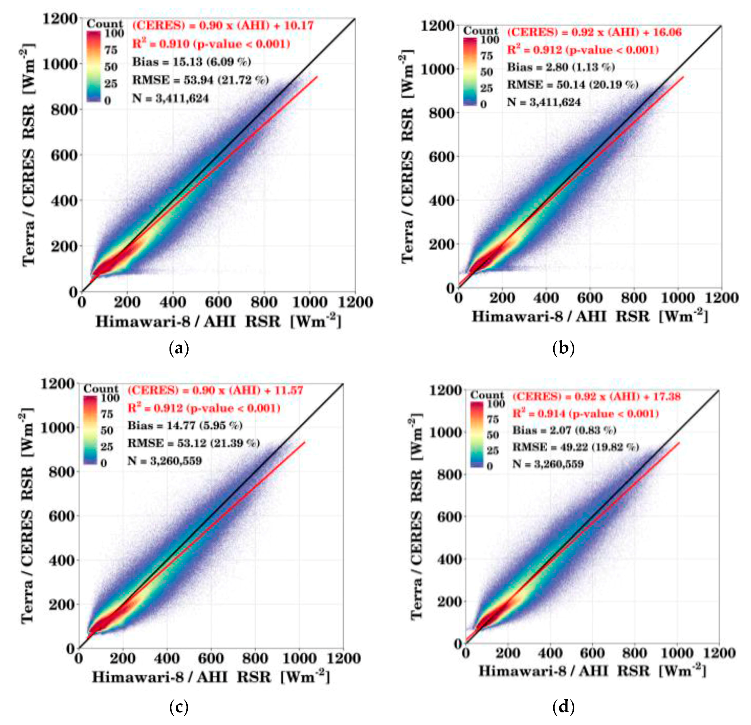
Figure 6.
Statistical analysis of RSR using Himawari-8/AHI and Terra, Aqua, and S-NPP/CERES data for the 15th day of each month from July 2015 to February 2017 (%Bias: blue dotted line; %RMSE: red dotted line; MPE: magenta dotted line; R2: cyan dotted line; Number: green bar chart). The legend shows the statistical results for the all case.

Figure 7.
Coefficient of determination (R2), standard deviation (Stdev), Bias, and RMSE of RSR using Himawari-8/AHI and Terra, Aqua, and S-NPP/CERES for the clear fraction for all cases. The bar graph shows the number of data.
Figure 7.
Coefficient of determination (R2), standard deviation (Stdev), Bias, and RMSE of RSR using Himawari-8/AHI and Terra, Aqua, and S-NPP/CERES for the clear fraction for all cases. The bar graph shows the number of data.
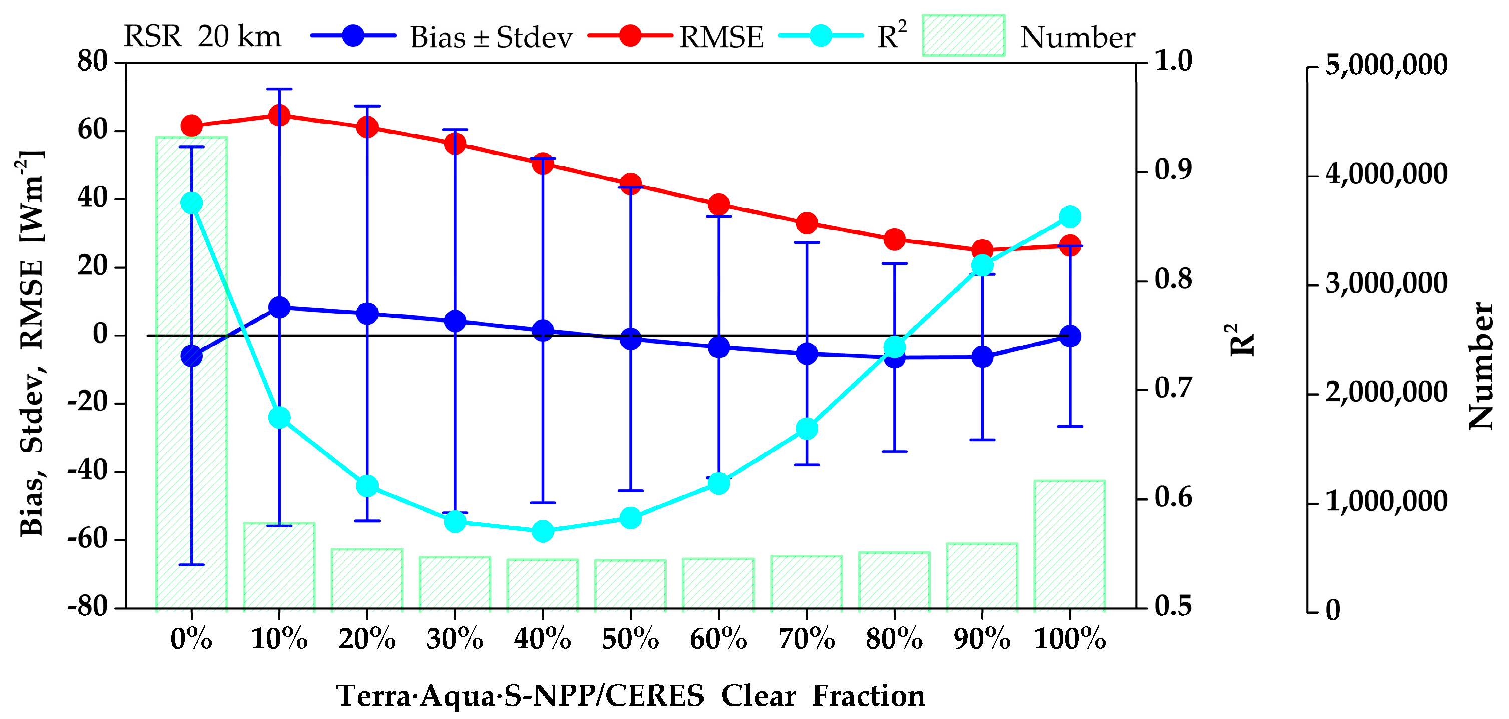
Figure 8.
Similar to Figure 6 but for validation data in: Terra (a); Aqua (b); and S-NPP (c).
Figure 8.
Similar to Figure 6 but for validation data in: Terra (a); Aqua (b); and S-NPP (c).
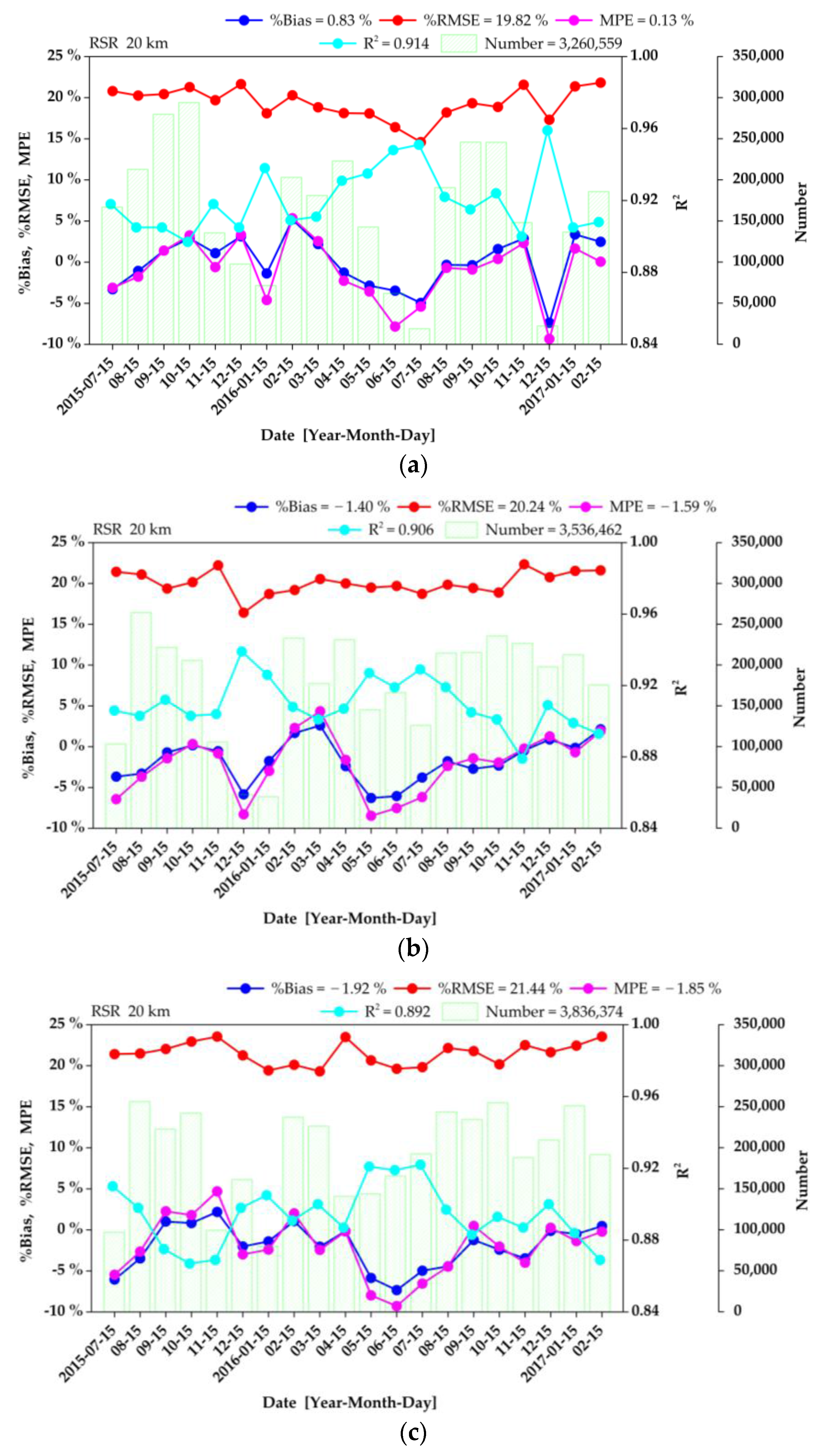
Figure 9.
Number of Terra, Aqua and S-NPP data compared to all data according to the clear fraction. Clouds were subdivided according to clear fraction (all: 0–100%; cloudy: 0–95%; clear: ≥ 95%; partly cloudy: 50–95%; mostly cloudy: 5–50%; overcast: < 5%).
Figure 9.
Number of Terra, Aqua and S-NPP data compared to all data according to the clear fraction. Clouds were subdivided according to clear fraction (all: 0–100%; cloudy: 0–95%; clear: ≥ 95%; partly cloudy: 50–95%; mostly cloudy: 5–50%; overcast: < 5%).
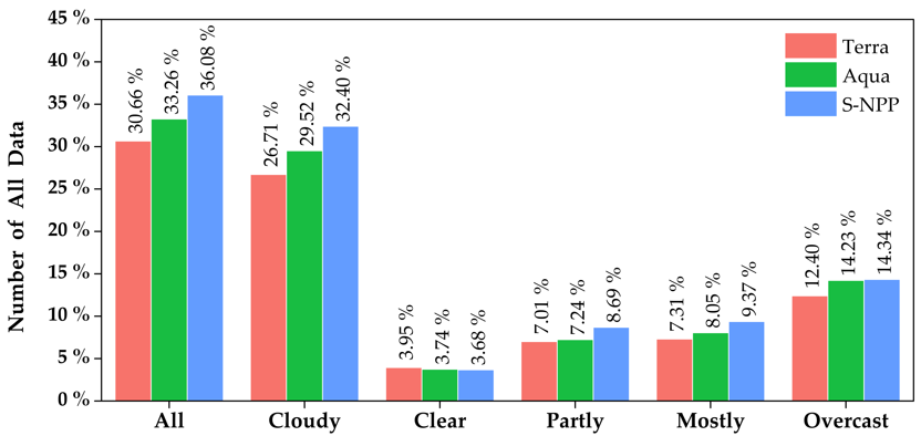
Figure 10.
RSR (Wm−2) of Himwari-8/AHI (left) and S-NPP/CERES (middle left) retrieved using data from the 15th day of every month between July 2015 and February 2017; percentage error (%) (middle right) and clear fraction (%) (right) between Himawari-8/AHI and S-NPP/CERES data sets; R2, Bias, and RMSE (top) between the two data sets.


Figure 11.
Similar to Figure 10, but for 20 km gridded mean (15 July 2015–15 February 2017) spatial distribution of RSR (Wm−2) from: AHI (a); and CERES (b); percentage error (c); and clear fraction (d). Mean RSR from AHI and CERES averaged along each latitude and percentage error on double y axis (e); and similar to but along each longitude and percentage error on double x axis (f).


Table 1.
Shortwave channel (CH) data from Himawari-8/AHI for retrieving RSR.
| Channel | Wavelength (µm) | Resolution | Main Purpose of Use | ||
|---|---|---|---|---|---|
| Spatial | Numbers of Pixels | Temporal | |||
| CH1 (Blue) | 0.47 (0.43–0.48) | 1.0 km | 11,000 | 10-min Full Disk | Weather forecasting Climate modeling |
| CH2 (Green) | 0.51 (0.50–0.52) | 1.0 km | 11,000 | ||
| CH3 (Red) | 0.64 (0.63–0.66) | 0.5 km | 22,000 | ||
| CH4 (NIR) | 0.86 (0.85–0.87) | 1.0 km | 11,000 | ||
| CH5 (NIR) | 1.61 (1.60–1.62) | 2.0 km | 5500 | ||
| CH6 (NIR) | 2.26 (2.25–2.27) | 2.0 km | 5500 | ||
Table 2.
Numerical experiments of SBDART for creating regression coefficient look-up-table (LUT).
| Parameter | Values Used for Look-Up-Table | Number |
|---|---|---|
| Spectral range | 0.2 to 3.3 at 0.005 µm | 620 |
| Solar zenith angle | 0°, 10°, 20°, 30°, 40°, 50°, 60°, 70°, 75°, 80°, and 85° | 12 |
| Viewing zenith angle | 0° to 85° at 5° increments | 18 |
| Relative azimuth angle | 0° to 180° at 10° increments | 19 |
| Atmospheric profiles | Tropical, Mid-latitude summer, Mid-latitude winter Subarctic summer, Subarctic winter, and US62 standard | 6 |
| Surface types | Ocean, Lake, Vegetation, Snow, and Sand | 5 |
| Aerosol types | Rural, Urban, Marine, and Tropospheric | 4 |
| Aerosol visibilities | 5, 10, 15, and 20 km | 4 |
| Cloud height | 2, 4, 6, 8, 10, 12, 14, and 16 km | 8 |
| Cloud optical thickness | 8, 16, 32, 64, and 128 | 5 |
Table 3.
Statistical results of TOA albedo using Himawari-8/AHI and Terra, Aqua, and S-NPP/CERES data.
Table 3.
Statistical results of TOA albedo using Himawari-8/AHI and Terra, Aqua, and S-NPP/CERES data.
| Date | Isotropy | Anisotropy | N | ||||||
|---|---|---|---|---|---|---|---|---|---|
| R2 | %Bias | %RMSE | MPE | R2 | %Bias | %RMSE | MPE | ||
| 15 July 2015 | 0.892 | 1.07 | 21.61 | 2.34 | 0.892 | −4.77 | 21.78 | −3.56 | 382,868 |
| 15 August 2015 | 0.881 | 3.99 | 22.99 | 4.98 | 0.882 | −2.80 | 21.98 | −1.72 | 765,902 |
| 15 September 2015 | 0.896 | 7.54 | 23.44 | 7.96 | 0.897 | 0.66 | 20.86 | 1.25 | 748,431 |
| 15 October 2015 | 0.894 | 8.17 | 24.55 | 8.65 | 0.889 | 1.27 | 21.94 | 2.60 | 769,128 |
| 15 November 2015 | 0.907 | 7.63 | 23.23 | 8.33 | 0.897 | −0.43 | 21.80 | 0.95 | 346,584 |
| 15 December 2015 | 0.894 | 4.08 | 21.94 | 5.37 | 0.885 | −1.74 | 21.56 | 0.00 | 318,051 |
| 15 January 2016 | 0.908 | 1.76 | 20.52 | 3.35 | 0.905 | −0.79 | 20.47 | 1.03 | 209,119 |
| 15 February 2016 | 0.904 | 8.13 | 22.09 | 9.47 | 0.899 | 1.39 | 19.73 | 3.56 | 700,569 |
| 15 March 2016 | 0.906 | 6.93 | 21.49 | 7.53 | 0.902 | 0.23 | 19.56 | 1.53 | 608,431 |
| 15 April 2016 | 0.900 | 4.43 | 22.57 | 4.63 | 0.900 | −1.18 | 21.15 | −0.54 | 622,010 |
| 15 May 2016 | 0.910 | −0.06 | 20.18 | −0.98 | 0.910 | −4.58 | 20.24 | −5.43 | 457,664 |
| 15 June 2016 | 0.895 | −0.91 | 20.07 | −0.98 | 0.897 | −6.11 | 20.33 | −6.32 | 414,194 |
| 15 July 2016 | 0.889 | 0.45 | 21.73 | 1.14 | 0.887 | −4.56 | 21.94 | −4.18 | 350,007 |
| 15 August 2016 | 0.880 | 4.25 | 23.00 | 4.54 | 0.891 | −2.65 | 20.73 | −2.47 | 673,663 |
| 15 September 2016 | 0.874 | 5.69 | 24.20 | 5.88 | 0.892 | −0.69 | 20.63 | −0.57 | 729,884 |
| 15 October 2016 | 0.900 | 5.59 | 22.04 | 5.78 | 0.900 | −0.81 | 20.05 | −0.12 | 769,781 |
| 15 November 2016 | 0.892 | 4.28 | 22.79 | 4.89 | 0.885 | −1.29 | 22.19 | −0.28 | 585,544 |
| 15 December 2016 | 0.900 | 3.49 | 21.33 | 4.86 | 0.892 | −0.59 | 21.17 | 0.92 | 451,665 |
| 15 January 2017 | 0.900 | 5.85 | 22.22 | 5.99 | 0.887 | −0.77 | 21.40 | 0.29 | 626,594 |
| 15 February 2017 | 0.887 | 9.59 | 25.63 | 8.82 | 0.878 | 0.94 | 22.14 | 1.36 | 578,772 |
| All | 0.893 | 5.16 | 22.67 | 5.58 | 0.893 | −1.14 | 21.04 | −0.33 | 11,108,861 |
Note: R2 is the coefficient of determination; %Bias is the relative Bias of (Bias/CERESMean) × 100 in percent; %RMSE is the relative RMSE of (RMSE/CERESMean) × 100 in percent; MPE is the mean percentage error of ((AHI-CERES)/CERES) × 100 in percent; and N is the number of pairs.
Table 4.
Statistical analysis of RSR retrieval results according to land, ocean, and clear fractions (all: 0–100%; partly cloudy: 50–95%; mostly cloudy: 5–50%; overcast: < 5%).
Table 4.
Statistical analysis of RSR retrieval results according to land, ocean, and clear fractions (all: 0–100%; partly cloudy: 50–95%; mostly cloudy: 5–50%; overcast: < 5%).
| Statistics | R2 | Mean | RMSE (%RMSE) | MPE | N | ||
|---|---|---|---|---|---|---|---|
| Clear Fraction Land & Ocean | AHI | CERES | |||||
| Cloudy | 0.869 | 302.70 | 313.46 | 56.02 (17.87) | −2.34 | 2,006,927 | |
| –Partly | 0.639 | 195.27 | 198.39 | 38.17 (19.24) | −0.25 | 574,000 | |
| Land | –Mostly | 0.657 | 270.61 | 277.79 | 59.52 (21.42) | −1.66 | 630,676 |
| –Overcast | 0.861 | 404.78 | 423.82 | 64.4. (14.97) | −4.36 | 802,251 | |
| All | 0.880 | 274.26 | 282.03 | 51.29 (18.29) | −0.51 | 2,632,865 | |
| Cloudy | 0.902 | 256.18 | 256.59 | 54.14 (21.10) | −0.60 | 7,417,530 | |
| –Partly | 0.429 | 105.49 | 111.12 | 30.62 (27.56) | −5.25 | 1,864,210 | |
| Ocean | –Mostly | 0.625 | 192.29 | 183.33 | 57.95 (31.61) | 3.98 | 1,999,843 |
| –Overcast | 0.874 | 371.19 | 374.14 | 61.12 (16.34) | −0.74 | 3,553,477 | |
| All | 0.909 | 243.16 | 244.24 | 52.39 (21.45) | −1.37 | 8,000,530 | |
Note: R2 is the coefficient of determination; Mean is the average in Wm−2; RMSE is the root mean square error in Wm−2; %RMSE is the relative RMSE of (RMSE/CERESMean) × 100 in percent; MPE is the mean percentage error of ((AHI-CERES)/CERES) × 100 in percent; N is the number of pairs.
© 2018 by the authors. Licensee MDPI, Basel, Switzerland. This article is an open access article distributed under the terms and conditions of the Creative Commons Attribution (CC BY) license (http://creativecommons.org/licenses/by/4.0/).
Share and Cite
MDPI and ACS Style
Lee, S.-H.; Kim, B.-Y.; Lee, K.-T.; Zo, I.-S.; Jung, H.-S.; Rim, S.-H. Retrieval of Reflected Shortwave Radiation at the Top of the Atmosphere Using Himawari-8/AHI Data. Remote Sens. 2018, 10, 213. https://doi.org/10.3390/rs10020213
AMA Style
Lee S-H, Kim B-Y, Lee K-T, Zo I-S, Jung H-S, Rim S-H. Retrieval of Reflected Shortwave Radiation at the Top of the Atmosphere Using Himawari-8/AHI Data. Remote Sensing. 2018; 10(2):213. https://doi.org/10.3390/rs10020213
Chicago/Turabian StyleLee, Sang-Ho, Bu-Yo Kim, Kyu-Tae Lee, Il-Sung Zo, Hyun-Seok Jung, and Se-Hun Rim. 2018. "Retrieval of Reflected Shortwave Radiation at the Top of the Atmosphere Using Himawari-8/AHI Data" Remote Sensing 10, no. 2: 213. https://doi.org/10.3390/rs10020213
Note that from the first issue of 2016, this journal uses article numbers instead of page numbers. See further details here.