A Holistic Concept to Design Optimal Water Supply Infrastructures for Informal Settlements Using Remote Sensing Data


Chair of Fluid Systems, Technische Universität Darmstadt, Otto-Berndt-Straße 2, D-64287 Darmstadt, Germany
*
Author to whom correspondence should be addressed.
Remote Sens. 2018, 10(2), 216; https://doi.org/10.3390/rs10020216
Submission received: 22 November 2017
/
Revised: 22 December 2017
/
Accepted: 26 January 2018
/
Published: 1 February 2018
Abstract
:Ensuring access to water and sanitation for all is Goal No. 6 of the 17 UN Sustainability Development Goals to transform our world. As one step towards this goal, we present an approach that leverages remote sensing data to plan optimal water supply networks for informal urban settlements. The concept focuses on slums within large urban areas, which are often characterized by a lack of an appropriate water supply. We apply methods of mathematical optimization aiming to find a network describing the optimal supply infrastructure. Hereby, we choose between different decentral and central approaches combining supply by motorized vehicles with supply by pipe systems. For the purposes of illustration, we apply the approach to two small slum clusters in Dhaka and Dar es Salaam. We show our optimization results, which represent the lowest cost water supply systems possible. Additionally, we compare the optimal solutions of the two clusters (also for varying input parameters, such as population densities and slum size development over time) and describe how the result of the optimization depends on the entered remote sensing data.
1. Introduction
The UN sets the goal to achieve universal and equitable access to safe and affordable drinking water for all by 2030 [1]. This addresses the 663 million people who do not have access to improved water sources [2] and at least 1.8 billion people globally who use a source of drinking water that is fecally contaminated [3]. A large proportion of these people lives in cities, as more than half of the world’s population currently resides in urban areas, with a tendency toward increase [4]. Currently, one quarter of the urban population (i.e., at least one eighth of the global population) lives in slums [5], which in particular are often characterized by inadequate water supply. Forecasts assume that the number of inhabitants of slums is still to increase in the next few years, especially in the world’s two poorest regions, South Asia and Sub-Saharan Africa [6]. This assumption is not far-fetched because slums develop very quickly. For example, the area of slums in Hyderabad, India, has grown by 70% within seven years [7]. The consequence of the lack of basic water infrastructure in slums is, among others, a high rate of child mortality [4]. Furthermore, the high expenditure of time that people invest in the procurement of water and in fighting diseases arising from contaminated water is a likely cause for them to have less time to spend on other essential issues, such as education and labor. In order to interrupt this vicious circle, it is necessary to provide people with water and to satisfy their basic needs. On this account, the goal to ensure access to water and sanitation is included in two of the 17 UN Sustainability Development Goals [1]. Goal No. 6 demands not only to ensure access to water and sanitation, but also supports and strengthens the participation of local communities in improving water and sanitation management. With Goal No. 11, the global community is aiming to make cities inclusive, safe, resilient and sustainable, and particularly to ensure access for all to adequate, safe and affordable housing and basic services, as well as to upgrade slums. For an adequate solution strategy to plan the infrastructure for a sufficient water supply, geographic information about the slums is necessary [8]. Both the spatial spread of these settlements, as well as their temporal development have to be mapped as precisely as possible. Hereby, two ways of measuring can be used: Until a few years ago, this was mainly based on censuses. These, however, require very large monetary and temporal resources. Additionally, censuses are often not accurate enough; for example, political influences can lead to distorted results [9]. Satellite data have proven to be a useful alternative for the detection and observation of slums due to the very high spatial and temporal resolution [10,11,12].
Based on remote sensing data, we developed a holistic approach combining different disciplines—such as mechanical engineering, mathematics and geography—to design an optimal water supply system for slums within an urban area. We apply methods of mathematical optimization and graph theory to find a network describing the optimal supply infrastructure. Hereby, we combine different decentralized supply approaches using motorized vehicles with centralized approaches based on the supply by pipe systems. The various means of water transportation must be modeled for which technical engineering expertise is necessary. In this paper, we bring together these different disciplines and also develop requirements for remote sensing resulting from this application.
This interdisciplinary approach consists of a framework with five main steps, which are illustrated in Figure 1, by which our expertise in particular lies within the latter three steps.
First of all, geographic information is gathered by remote sensing. In the second step, the gathered data need to be analyzed and slums need to be classified. These two steps are further detailed in Section 2.1. The cost model for the design of a water supply network is given in Section 2.2. Here, we explain the cost functions and how the results from slum classification are processed as input. Next, in Section 3, the cost model is translated into a mathematical modeling language to create a mixed-integer problem (MIP), which can be solved by state-of-the-art optimization software. In the last step of the introduced framework, the solution of the MIP, i.e., the result of the optimization, is converted into a graphic illustration to display the results in an easily interpretable form. For the purposes of illustration, we apply the approach to two small slum clusters in Dhaka and Dar es Salaam. This choice is backed by the fact that a large proportion of the inhabitants of slums lives in Sub-Saharan Africa and Asian countries [6]. Section 4 presents these optimization results, which represent the lowest cost water supply systems possible. We also compare the optimal solutions for the two different cities, as well as for varying input parameters, such as population density and slum development over time. However, the aim of this paper is to introduce a tool to optimize the water supply, which we kept very flexible regarding input data, rather than recommending to build the exemplary water supply systems as shown. For detailed planning of a system, we would advise (and offer) to re-run the optimization with more accurate information in regards to the costs provided by potential users. Finally, we discuss the influence of different factors and the entered remote sensing data on the optimization result in our discussion in Section 5. These factors are also displayed in the framework in Figure 1.
2. Materials and Methods
This section details the first three steps of the introduced framework in Figure 1. Section 2.1 captures the first two steps by describing how the geographic information is gained using remote sensing and how slums are identified. The third step of the framework specifies the cost model in Section 2.2.
2.1. Remote Sensing, Slum Identification and Test Sites
With the rising number of launched very high resolution (VHR) sensors and thus the amount of available VHR image material in the last few years, the number of publications about the classification of slums (methods and case studies) has also increased [5]. In order to classify slums using remote sensing data, the first step is to give a definition and to derive suitable features for their classification.
Previously, we used both terms: informal settlements and slums. While the term informal settlement is used for urbanized areas in the context of municipal planning efforts [10], the term slum is defined as an area, where at least one of the following five criteria is fulfilled: lack of access to safe water, lack of access to improved sanitation, lack of tenure, overcrowding or non-durable housing [4]. Both terms open up a wide range of possible interpretations. Although they cannot be used synonymously, the two terms contain a large common intersection [10]. In the following, we will use the term slum for the areas in urban regions in which the poor population lives in bad conditions, assuming that there likely is a lack of access to safe water, which has to be improved.
Note that only one of the five above-mentioned features of a slum, non-durable housing, can be detected by remote sensing [5]. Furthermore, most slums around the world show different characteristics depending on their localization [5,13], e.g., regarding height or roof material. For example, slums in Mumbai are usually one-story, while favelas in Sao Paulo are mostly two-story [13]. Yet, it is possible to identify similarities between slums, as well as to identify differences from formally built-up areas and use these to detect and map the size, as well as the growth of slum areas [5]. Differences from formal areas can for instance be found in several features such as size (small building sizes vs. generally larger building sizes), density (especially the roof coverage density), pattern (organic vs. regular) or size characteristics [5].
There are many methods for the identification of slum areas such as the object-based approach, texture, morphology or visual image interpretation [5]. Due to the nowadays high resolution of the image raw data, which reaches values of m (WorldView-3, launched in 2014, Ball Technologies Holdings Corp., Boulder, CO, USA ), the different slum areas around the world can be detected very precisely (area based image analysis) with accuracies of up to 98% [14]. It is even possible to detect single objects (houses, roofs) by object-based image analysis. For object-based image analysis, the sensors have to fulfill particular requirements specified by Jacobsen and Byuksahli [15]: for the detection of houses, a resolution of <2 m, of footpaths 1–2 m and for detailed building information <0.5 m are necessary. These requirements are based on formal housing and require an adjustment to apply them to informal settlements in order to reflect the growth stage of the slum area and related high density of the roofing structure.
To illustrate our method, we apply the approach to two small slum clusters in Dhaka, Bangladesh (for the years 2006 and 2010) [11], and Dar es Salaam, Tanzania (for the years 1998 and 2002) [16]. Both input datasets are open-access and have been created using remote sensing data. The raw data for the classification for Dar Es Salam were generated using SPOT satellite (10 m) and SFAP (35 mm at a 500–800-m height) images. The classification for Dhaka is based on QuickBird satellite images with a resolution of 0.6 m, complemented by data from the 2005 census and mapping of slums, Google Earth data (IKONOS; SPOT and QuickBird) and geolocated photographs. To avoid small and isolated slums, the data were filtered in GIS [11]. We used the data about the informal settlements provided in shapefiles and calculated the centers of the slums to identify the distance between the slums, as well as the area of the slums via MATLAB [17].
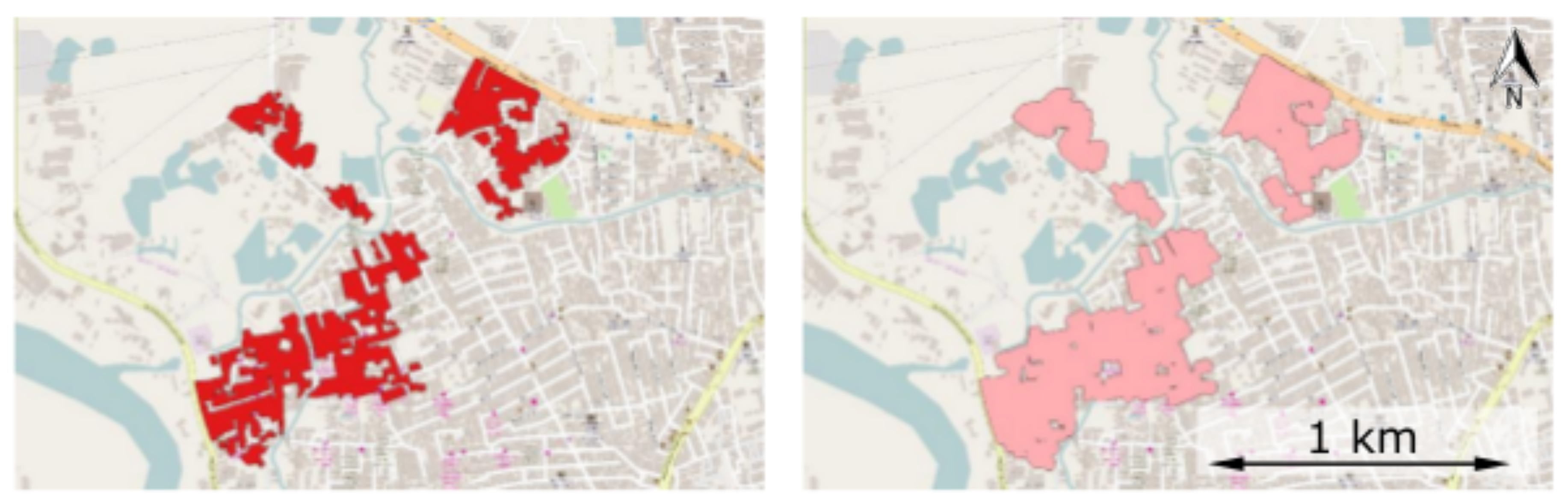
In our study, we investigate the influence of different parameters on the optimization result in order to provide recommendations for later data surveys in remote sensing. Firstly, we investigate the impact of the data resolution on the result of our approach. To do so, we simulate a lower spatial resolution of the data by adding an artificial buffer of 10 m, hence blurring borders and inaccurately mapping slums, and compare the optimal water supply infrastructure for higher and lower data resolution (see Figure 2).
Secondly, we investigate the influence of a varying population density by varying this input parameter value in the cost model. The population density is one of the most uncertain input parameters in our cost model. While we can get information about physical parameters like roof color, roof sizes or densities out of remote sensing data, there is no direct information about the slum population. In this work, we estimate the slum population by multiplying the slum area by an average population density. However, we note that estimates of the population densities in slums are still subject to high uncertainty. An example of this fact is Kibera, Nairobi, in Kenya. The area of Kibera is km. While it is one of the best known slums in the world, the population estimations differ from 160,000 inhabitants up to 640,000 inhabitants, corresponding to a population density range between 64,000 and 256,000 persons per km [18], which is equivalent to a factor of 4.
Since the number of inhabitants is a key value for infrastructure planning, it would greatly benefit from more precise estimations of the population in slums. Some studies try to improve the estimation of the population by using three-dimensional data of slums [19]. However, this has only been done for a few case studies, and the data are not freely available. As Kuffer et al. recommend, a uniform database on slums [5], which can be used for applications like the one presented here, would be of high value. It would be helpful to have an exact depiction of the environment, including the infrastructure (size of bridges, etc.).
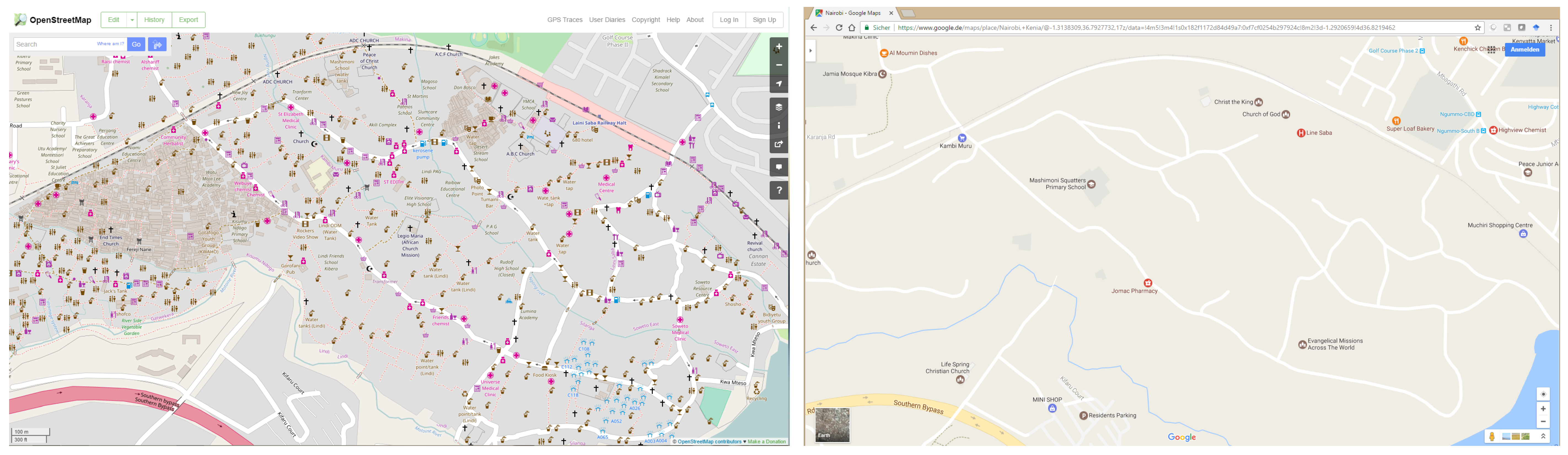
At this point, it is clear that remote sensing is only intended as a support, but it is always necessary to interpret and enrich the data through local knowledge. This inclusion of local knowledge, in contrast to or on top of authoritative sources, is also dealt with in volunteered geographic information (VGI) platforms. A prominent VGI example is OpenStreetMap [20]. Figure 3 illustrates the contrast of different sources for Kibera, a slum in Nairobi, by showing the very detailed map from OpenStreetMap (right) compared to Google Maps (left).
Another project worth mentioning is MapKibera [21] where Kiberans created the first free and open digital map of their own community. The quality of such non-authoritative sources is compared with authoritative sources in [22] for road datasets in Nairobi. The possibility of exploiting VGI as potential practices for gathering spatial information about informal settlements is discussed in further detail in [23].
2.2. Cost Model
The aim of the presented approach is to design the water supply infrastructure for all slums within one large city. We model the water supply system as a network that provides each slum with the required amount of water. To calculate this required amount, the sizes of the slums are calculated in MATLAB based on the provided slum classification. Using these data, the daily water need for each slum is calculated by multiplying the slum size with an estimated population density and the daily need per person. In the current model, one water delivery point in each slum needs to be supplied. The water distribution within each slum is considered in a separate research project. We include sources in the system, waterworks, to provide the required amount of water. The coordinates of the sources can be entered as input parameters in the model, based on the availability of water sources in the city. These sources do not have to be real waterworks, but could also be locations in the existing water supply system of the formal settlements that have a surplus of water. In addition, the decision where to locate water sources can be included in the optimization by inserting several possible waterworks and checking in the results which waterworks are used. From these waterworks, every slum can possibly be supplied by building a connection from the waterworks to the individual slum. To reduce the total length of the connections, slums can also function as intersections. Hence, all connections between any two slums of the city are added to the set of possible connections. Therefore, the network is modeled as a directed complete graph [24]. An illustration of the directed complete graph with four vertices is shown in Figure 4.
The vertices of the graph represent the slums and the waterworks, whereas the edges represent the possible connections between them. On each edge, different connections can be selected: the water can be transported via a variety of pipes with different diameters or via a selection of motorized vehicles (e.g., trucks or mopeds with different capacities). While making these design decisions, the objective is to reduce the overall costs over a specified period of time, including investment, as well as operating costs.
The tank costs are inserted as input parameters, whereas the costs for trucks and pipes between two slums i and j with distance are calculated with the following functions using the input parameters from Table 1.
The costs for the supply via trucks is calculated for each available truck type k individually by:
This function contains the factor 365 for the number of days of a year and the factor 12 for the months. Additionally, the calculation of the truck driver’s wage is multiplied by the factor 2, assuming that two drivers are required to cover every day of a year. The costs for pipes are split into fixed costs, the investment to buy and install the pipes [25] and variable costs for the operation, which depend on the volume flow within the pipe. This dependency is caused by the energy consumption of pumps, which are required to transport the water through the pipe network. Since this study on fixed pipe costs [25] was conducted in Portugal, we multiply these costs by a factor representing the difference in the overall price level between Portugal and the target country (e.g., the GDP ratio). The fixed costs of a pipe with diameter d are calculated by:
In the optimization model, the volume flow on each edge is a decision variable that is to be set by the optimizer. To linearize the variable costs, we calculate the factor for each pipe diameter and length in the pre-processing with Equation (3). In the optimization objective function, this factor is multiplied with the cubic volume flow to calculate the variable costs for pipes. To calculate this factor, we apply the common dissipation model with pressure loss and pipe length l leading to variable costs . Excluding from these terms, the variable cost factor for the optimization model is calculated by:
This leads to the total costs of a pipe given by:
In addition, the chosen connections need to provide a sufficient capacity to carry the required amount of water. The capacity is evaluated on a day to day basis. The capacities of trucks and tanks are inserted as input parameters, whereas the capacity of pipes is calculated depending on the inserted pipe diameter d:
The factor 3,600,000 in Equation (5) is split into two parts . The first part is given to convert seconds into hours. The factor 1000 is used to convert the capacity calculated in cubic meters into liters. Further requirements ensure the full functionality of the water supply system, such as flow conditions, which demand the incoming flows for each slum to equal the sum of outgoing flows and internal daily need.
Furthermore, tanks are required in a slum if water is carried by trucks into the slum or out of the slum. Hence, these tanks need to provide sufficient capacity for the following four volume flows (see also Figure 5):
(I) Water delivered by a truck, (I-a) for the daily need of the slum itself , (I-b) to be carried onward by truck or (I-c) to be carried onward by pipe and (II) water coming into the slum by pipe and then being carried onward by a truck ().
To reduce the overall tank capacity, the following prioritization logic is applied for water coming in by pipe . First, continuing from pipe , the remaining water is used for the slum itself . The remaining water is then carried further by truck .
In an advancement of the model, geographic barriers, like rivers or narrow roads, prevent specific connections. This information is inserted into the model as input for the individual connections. It is possible to distinguish the prohibition of every single type of connection, e.g., one can allow a connection between two slums for a small moped, but forbid it for a large truck because the road between the two slums is to narrow for a truck. This advancement improves the degree of authenticity of the model, but also increases the complexity of the optimization model. Furthermore, the data on such barriers need to be processed in such a way that they determine for any connection, i.e., any combination of two slums with any supply type, if the connection is valid or blocked by a barrier.
3. Theory and Calculation
3.1. Introduction to Optimization and Technical Operations Research
In photogrammetry and remote sensing, optimization techniques have been specifically applied for the modeling of buildings. Related to our work, two publications are to be mentioned in particular. In the first one, informal settlement areas are the subject of research, as well, but a different optimization technique, the dynamic programming optimization, is applied to semi-automatically extract buildings from aerial photographs [26]. The second one uses the same optimization method as we do, mixed-integer linear programming (cf. Section 3.2), but applies it to the aggregation of the first level of detail (LoD 1) building models [27]. While in the two mentioned works, optimization techniques are applied to optimize the extraction of information from remote sensing data, in our approach, optimization is used in a subsequent step: we optimize the design of an infrastructure, a water supply system, using already classified remote sensing data as an input.
The optimization of this water supply system is based on technical operations research (TOR). TOR is an approach for the design of technical systems that allows one to find optimal system structures based on discrete optimization [28]. The aim of the method is to provide models and algorithms for structuring complex technical systems. The TOR approach has already been used to optimize various technical systems such as heating or ventilation systems [29,30] or the drinking water supply for buildings [31]. TOR is based on techniques known from the field of operations research, which have already been successfully used in logistics, production planning or scheduling [32,33] and are now also applied to structure technical systems. In this new context, techniques from discrete mathematics allow the optimal synthesis of technical systems with the help of algorithms [34,35].
3.2. Basics of Discrete Optimization
Finding an optimal design of a water supply system is an optimization problem that contains discrete decisions (e.g., rather choose a pipe or a truck on a certain section of the network?), as well as continuous physical constraints (e.g., hydraulic resistance laws). Thus, a mixture of discrete (binary) variables modeling the discrete decisions and of continuous variables describing physical quantities, like pressure or volume flow, arises. Such optimization problems can be modeled as mixed-integer linear programs (MILP) [36] and solved by state-of-the-art commercial solvers like CPLEX [37] or Gurobi [38].
The variables in the MILP are selected by the optimization solver such that, on the one hand, all constraints can be satisfied and, on the other hand, the objective value, measuring the total costs, is minimized. The structure of this optimization problem can be represented by a decision tree (cf. Figure 6a). Any discrete decision for or against the use of a certain pipe or truck on a section of the water supply network leads to a new branch of the decision tree. The leaves of the tree represent the different layout options for the water supply network. The number of solutions can quickly become too large to assess and compare them manually, given a realistic problem size. While some of the numerous leaves of the decision tree do not represent valid solutions (e.g., since these layout options are not able to provide the required water supply), others could be chosen to build the system. These valid solutions are called primal solutions of the optimization problem and may be “good” or “bad” with regard to the objective function.
During the exploration of the decision tree, the quality of the primal solutions found increases, cf. Figure 6b. Due to the specific formulation of the optimization problem, additional information can be generated that allows us to find a proven global optimal solution and not only a local optimal one: a so-called dual bound can mathematically be derived. This indicates how good the best solution could possibly be and is continuously tightened during the optimization process, i.e., converged towards the primal solution. If a primal solution and the dual bound meet, a solution is found that cannot be improved any further, even if the decision tree has not yet been explored entirely. Thus, the discrete optimization using TOR provides a global optimum as opposed to other optimization strategies such as genetic algorithms or gradient-based optimization methods.
3.3. Developed Optimization Model
Modeling a given application scenario requires a systematic approach since all boundary conditions must be known prior to the optimization.
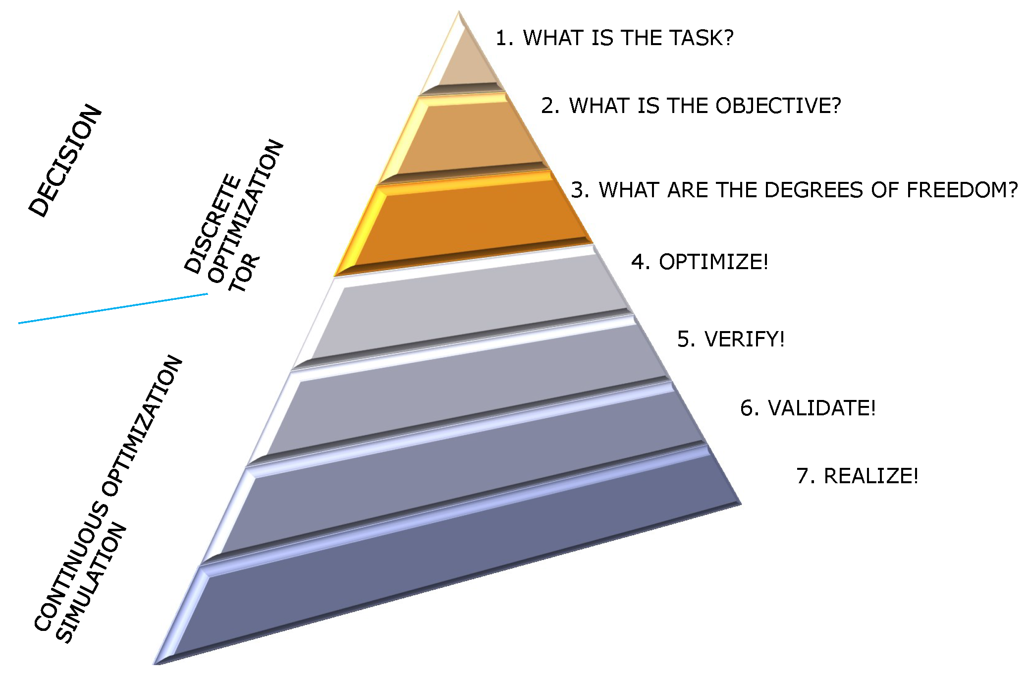
The TOR pyramid (cf. Figure 7) illustrates the individual steps of the approach [28]. The first four steps are treated using the application of planning an optimal water supply system for informal settlements in Section 3.3.1, Section 3.3.2, Section 3.3.3 and Section 3.3.4 by translating the cost model, which was introduced in Section 2.2, into an optimization problem. We also commence the verification, Step 5, in the analysis and discussion of our optimization results in Section 4 and Section 5. The last two steps would require a great effort since the designed application examines a tremendous system, compared to former applications of the TOR approach.
3.3.1. What Is the Task?
The first step is to describe the function of the system to be optimized. In the case of the water supply system, the function is given by a volume flow within a network that supplies each slum with a required amount of water, as already described in the cost model in Section 2.2.
3.3.2. What Is the Objective?
The second step is to define the objective of the optimization. This objective is always subjective. In the application example treated here, we minimize the total costs, including investment and operating costs, within a fixed operating term of five years in Equation (A1). Furthermore, it is possible to adjust the objective by adding weights in the objective function to reflect the preferences and relevance of different stakeholders. For instance, the operational costs related to environmental pollution (e.g., fuel, power for pumps) could be reduced by multiplying them with higher weights than the other costs. This would allow higher investment costs as a trade-off for lower environmental pollution.
3.3.3. What Are the Degrees of Freedom?
In this third step, the degrees of freedom for the structure of the technical system are described. In our case, the optimization algorithm may choose to install pipes or use trucks to provide water. The pipes can be chosen out of a set of pipes with different discrete diameters, and the trucks also come in different sizes. In the optimization model, the degrees of freedom are the decision variables and can be found in Table A2.
All inter-dependencies of the variables and parameters, describing requirements to fulfill the task, as well as the degree of freedom, are captured in the constraints of the optimization model. In this water supply design model, the constraints induce the following conditions (for ease of readability, we only give a textual description in this section. However, the mathematical representation of all constraints can be found in the Appendix A): The volume flow on an edge is the sum of the volume flows via pipes and trucks, which is calculated in Equation (A2). The flow condition requires that the total incoming volume flow equals the sum of outgoing flows and daily need for each slum in Equation (A16). The capacity of a connection needs to exceed this volume flow on the corresponding edge in Equations (A3) and (A4). Pipes and trucks can be chosen if and only if the connection between the two slums i and j is used. Additionally, the number of trucks per edge is limited by , and only one pipe is allowed per edge in Equations (A5)–(A7). Since the costs in the objective function scale cubical with the volume flow, a linearization is required and is here modeled with the constraints of an incremental linearization method [39] in Equations (A8)–(A12). Furthermore, a slum cannot supply itself, therefore loops are not allowed in Equations (A13)–(A15). The prioritization logic for the tank capacity calculation is represented by the following three relationships: Firstly,
which is modeled in Equations (A20)–(A22) by applying a BigM-method [40]. Secondly,
is represented in Equation (A23). Thirdly,
which is modeled in Equation (A24). For the second and third equation, only the lower bounds of the maximum relation need to be modeled since the variables are automatically pushed down as far as possible by the objective function. The last pending value is calculated in Equation (A25). Based on these calculations, the tank capacity requirement in each slum, which can be provided by a number of tanks, is given in Equation (A19). Additional constraints set all volume flow variables to zero if the corresponding edge is not used in Equations (A26)–(A28).
In the model extension with geographic barriers, the compliance with these requirements is modeled in Equations (A17) and (A18).
3.3.4. Optimize!
After defining the function, objective and degrees of freedom, the optimization algorithm finds an optimal system structure under these conditions. The optimization is carried out considering not only one single model of one concrete system structure, but considering all possible system structures at once.
4. Results
To illustrate the above introduced model by means of a practical example, we look at two selected slum clusters in Dhaka, Bangladesh, and Dar es Salaam, Tanzania. With these cities, we cover two regions with a higher occurrence of slums, Sub-Saharan Africa and Asia. Additionally, we can demonstrate that the approach is applicable independent of the region. Both cities also show a high variation in urban, as well as slum population, which we include in the analysis of the impact of time. Please note that the input data used in these examples were collected to the best of our knowledge, especially in respect to costs and price levels in the different countries. Due to this fact, we prefer not to state the overall costs to prevent the suggestion of a misleading degree of accuracy. However, the comparison of the optimization results, in the form of the resulting networks, is reasonable since the same underlying information has been used for all shown examples. Furthermore, the benefit of this optimization model is that it is flexible regarding input data and can be re-run easily if better data are available.
In the following, we show the results for different instances of these two slum clusters. In general, all input data are kept the same except for the one specifically stated indicator.
4.1. Optimal Water Supply for Two Cities
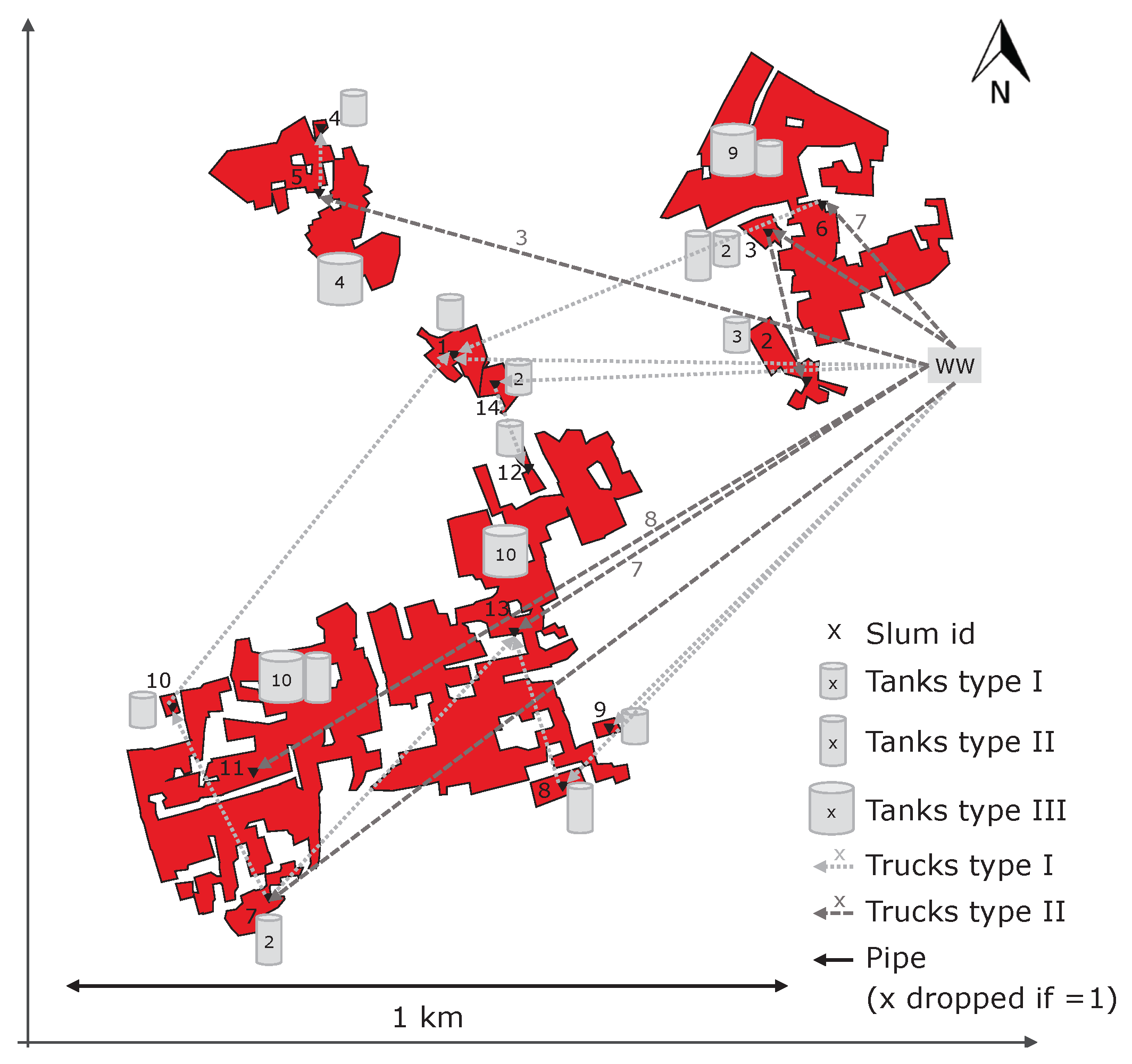
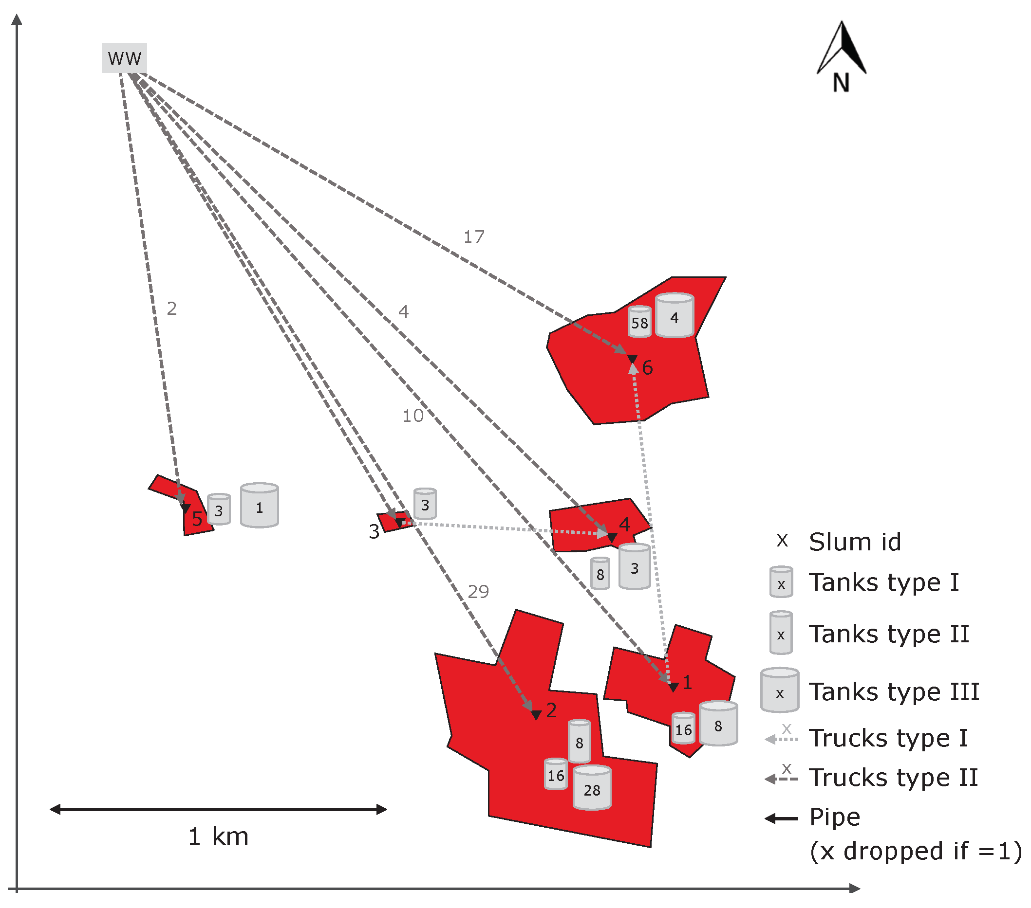
Firstly, the basic results for the two slum clusters are presented here. In the following figures, slums are numbered with an id and the slum area is outlined in red. The waterworks is represented by a grey box, which is labeled with “WW”. For each slum, the chosen tanks of different sizes are displayed with cylinders. The selected connection types are represented by arrows of different colors and dash types that point towards the slum center. Both tanks and connection are tagged with the respective number if more than one is selected.
In Figure 8, the optimal supply systems for a cluster in Dhaka with 14 slums in the year 2010 is shown, which was already introduced before in Figure 2. For this example, the result of the optimization is to not install any pipes, but to operate only trucks of different types. This can be explained by the short time period of five years that was considered in this application example. Within five years, the investment costs for a pipe system may not yet pay off. Nevertheless, one can see in this example that slums function as a point of transfer for subsequent slums, for example Slum 5 for Slum 4.
In an area of four-times the size as shown above for Dhaka, there are still only six slums in Dar es Salaam in the year 2002. The resulting optimal water supply network, shown in Figure 9, consists of a far less complex network due to the lower number of slums.
4.2. Impact of Time
For both slum clusters, the change of slum area over time becomes visible when comparing the two introduced examples with remote sensing data from a previous point in time.
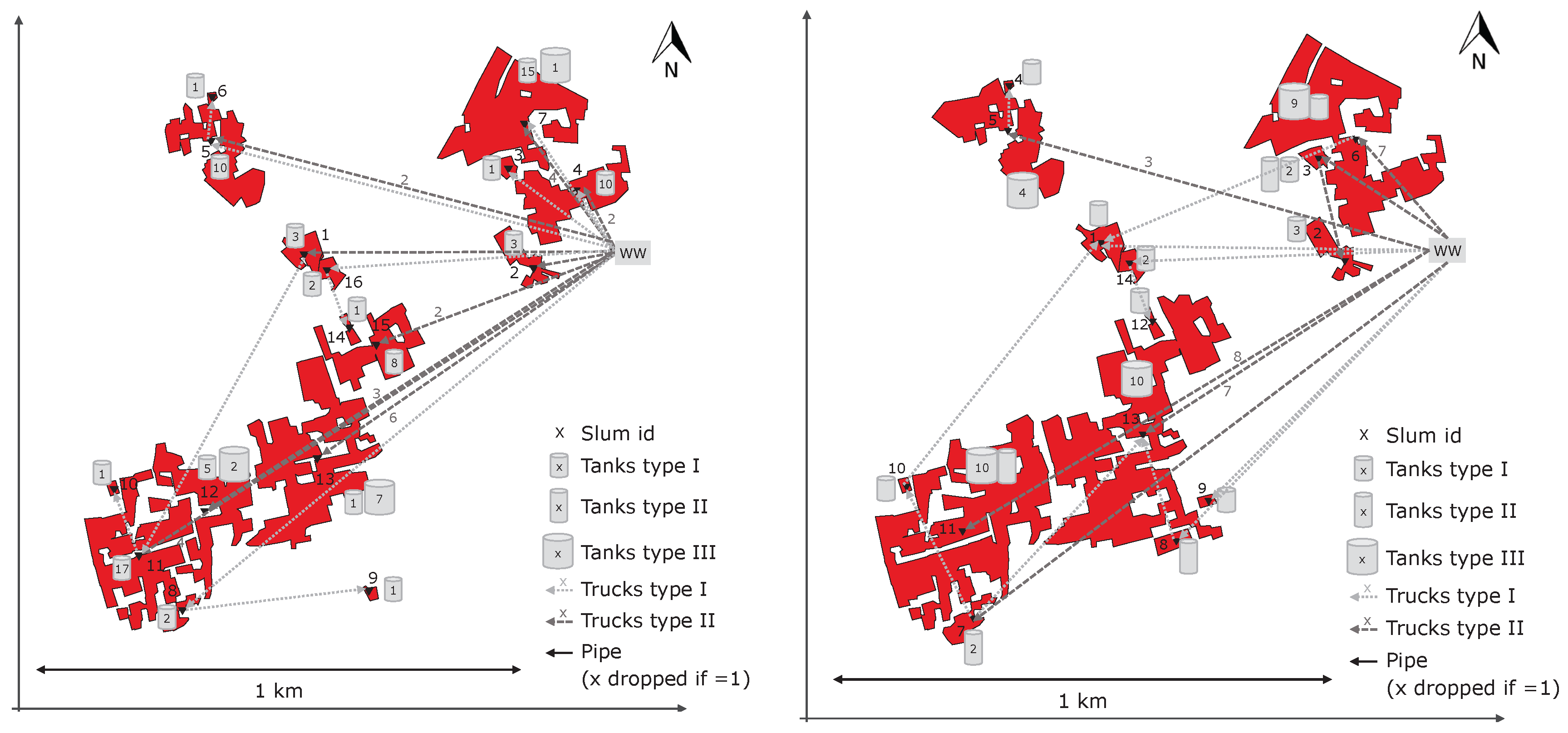
The additional data for Dhaka are from 2006, cf. Figure 10 (left), leading to a difference of four years between the two recordings. One can see that Slums 14 and 15 in 2006 became one slum in 2010. Similarly, Slums 11 and 12 became one slum. One slum, Number 9 in 2006, disappeared, and two new slums, Numbers 8 and 9 in 2010, formed over time. Overall, this reduced the number of slums observed within the selected slum cluster from 15 slums in 2006 to 14 in 2010. The supply connections for the unchanged slums remain fairly stable, whereas the choice of tank types changes more severely.
In Dar es Salaam, only two slums existed in 1998 and four slums emerged in the four years between the two recordings (see Figure 11). Nevertheless, the two lasting slums changed only slightly, as well as their supply.
An option to deal with this development over time is to include an estimate of the population in the optimization model aiming to design an infrastructure, which also copes with future needs. Two ways are possible for this, either to use the estimated future population size in the current model or to introduce different scenarios (with different future populations sizes) with a likelihood of occurrence in the optimization model.
4.3. Impact of Varying Population Densities
Since the population density is an input parameter that is very difficult to estimate, the impact of varying input population densities is demonstrated in the following example.
Figure 12 (right) shows the optimal supply system for Dhaka in 2010 for a reduced population density of 50,000 people per km, whereas in all previous and following examples, a population density of 100,000 people per km was assumed, also in Figure 12 (left). As these results show, the model is quite sensitive in regards to the population density. Therefore, remote sensing data with information on the individual houses could increase the accuracy of the density estimate and consequently of the optimization results.
4.4. Impact of Varying Resolution
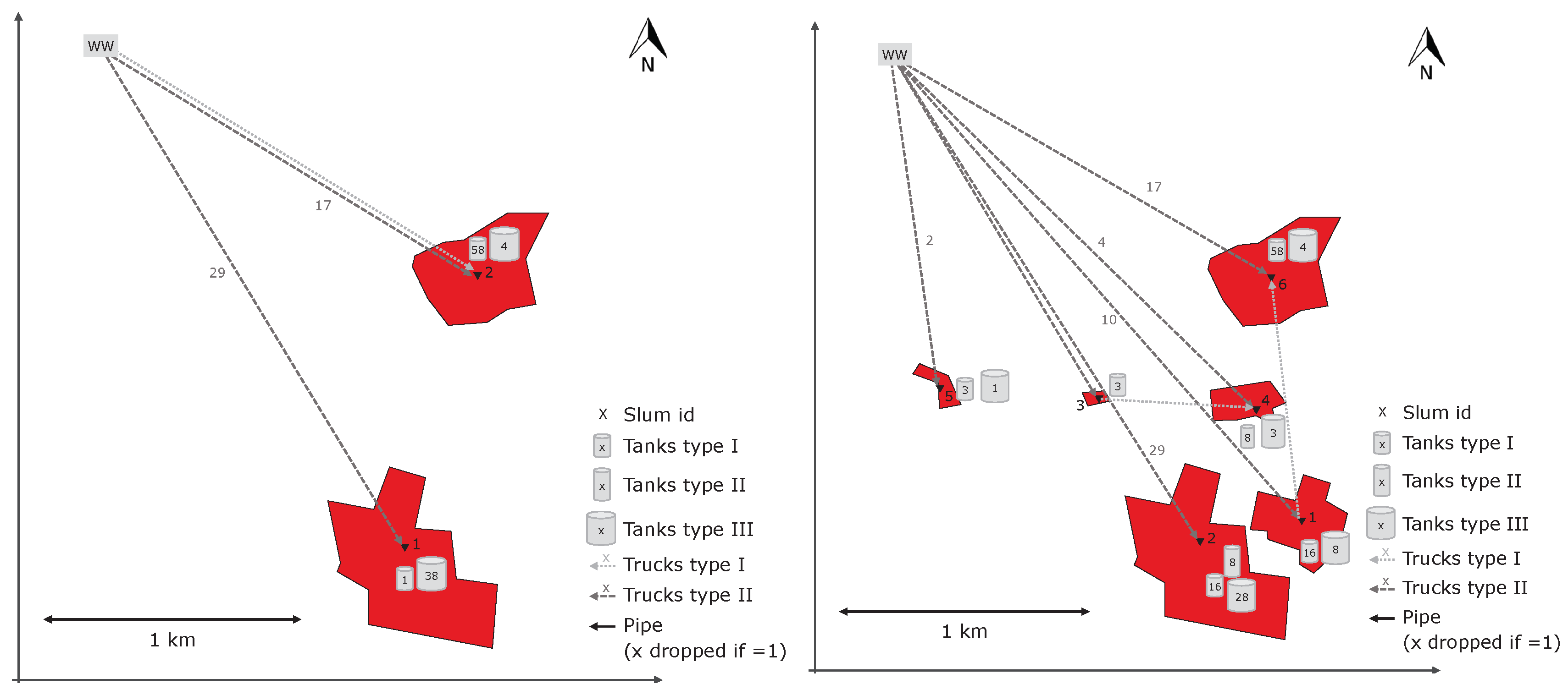
To imitate different resolutions of the remote sensing data, a buffer was introduced. With this buffer, all slums with a minimal distance of less than the buffer size were consolidated into one slum, assuming that a lower resolution would have made it impossible to identify the individual nearby slums. Figure 13 (right) shows the previously introduced example of Dhaka in 2010 with an added buffer of 10 m, which leads to only five identified slums and hence a large difference in the total slum number compared to the original with 14 slums.
The higher resolution in Figure 13 (left) leads to spatially better spread tanks, whereas the simulated lower resolution leads to a concentration of tanks in the center of the consolidated slum set. This increases the transportation distance within the slum set itself, which is currently not included in the optimization model due to the fact that structured planning within a slum is even more difficult to enforce. Hence, by using a higher resolution and due to the consequential disaggregated analysis of the individual slums, this transportation can be taken into account already during the optimization.
4.5. Geographic Barriers
To simulate geographic barriers, which could also be identified with remote sensing data, we added additional constraints blocking specific truck connections.
In Figure 14 (right), the results are shown for Dhaka in 2010, considering a river (blue line). The result is a very entangled network including pipe and truck connections, which adheres to the barrier restriction and corresponds to the cost-optimal solution, but would have to be reconsidered from an engineering perspective due to its high complexity.
4.6. Impact of Varying Calculation Periods
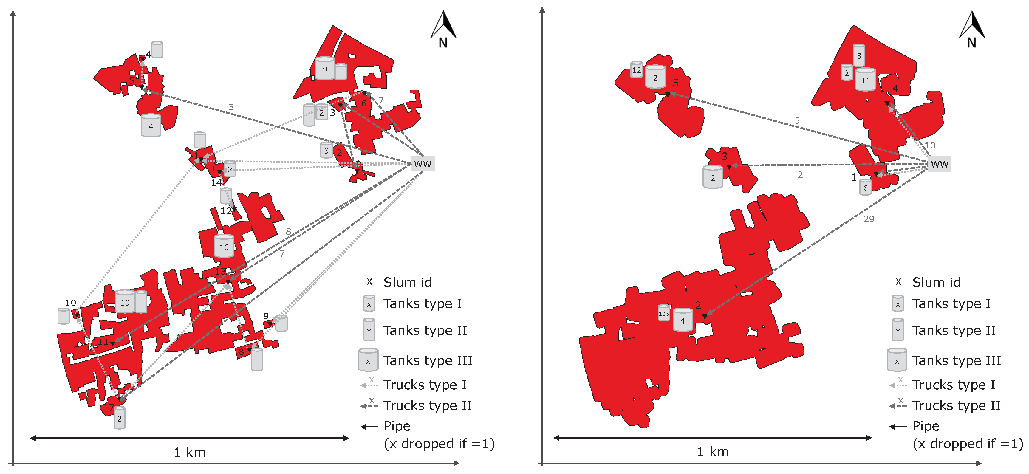
The optimization result also depends on the time period under consideration since the effect of the operating costs compared to the investment costs increases with a growing number of considered years. The impact of this input parameter is illustrated in Figure 15, which shows the results for a period of five years (left) and for a period of 15 years (right).
In the previously shown results, a period of five years was chosen to take into consideration the dramatic changes in slum areas over time as described in the introduction for Hyderabad where the area of slums has grown by 70% within seven years [7]. This change can also be observed in the comparison of the results for different points in time in Section 4.2. Nevertheless, the period parameter can be adjusted for each optimization depending on the preferences of potential users and their planning horizon.
The results show that for a longer period, the number of connections with smaller trucks and from the waterworks declines. This is caused by the reduced impact of higher investment cost for larger trucks and by the increase of the impact of operating cost, which are mainly driven by the distances.
5. Discussion of Optimization Results
Reflecting upon the results shown in the previous section, the key advantages of using remote sensing to reach global sustainability goals become apparent: the high spatial and temporal resolution. Thanks to the high resolution data and the advances in the classification of slums, it is possible to retrieve high quality input data for planning optimal water supply systems for slums. By recording physical parameters, such as building area and the optical characteristics of roofs, the location and temporal development of informal settlements can be derived. Yet, another key input parameter in planning the optimal water supply infrastructure is the population size, which is required to calculate the water need. Based on the current techniques, the population size can only be estimated roughly by multiplying an estimated population density with the identified slum area.
As expected, the population density has a high impact on the optimal infrastructure design. This is observable when comparing the different optimization results for the same slum cluster with identical input parameters except for the population density (cf. Section 4.3). Unfortunately, there is no consistent and reliable data on population density available in most areas of the world. These estimations would be improved significantly by models based on 3D mapping. An improved estimate of the population size could be included in our introduced optimization model easily.
An additional influence factor for the resulting infrastructure topology is comprised by barriers, which were included in the model in Section 4.5. These results show that the model can handle restrictions caused by geographic barriers, for example rivers, which prohibit the usage of connections between specific slums. Currently, these barriers are added manually. Therefore, it would be a great improvement to leverage land use information provided by remote sensing as input data, including road networks, hydrographic features, topographic features, etc. These data would need to be processed in such a way that they indicate for any connection if it is blocked by a barrier.
Furthermore, the impact of the spatial resolution of the remote sensing data on the optimization results is notable. This is shown in Section 4.4, where we imitated different resolutions of the input remote sensing data by adding a buffer to cluster very close slums and investigated the impact of the resolution on the optimal infrastructure design. Logically, a higher resolution yields to a better fit of the solution to the real conditions. With a lower resolution, different slums were detected as one single slum, even if barriers between the slums exist and a supply from one slum to the other is not possible. Additionally, an inferior resolution would influence the population size estimation causing a miscalculation of the water need.
6. Summary and Outlook
In this paper, we introduced a holistic framework to design optimal water supply infrastructures for informal settlements using remote sensing data. Therefore, this work shows an opportunity to leverage remote sensing data to contribute to achieving the UN Sustainability Development Goals, especially Goal No. 6: “Ensuring access to water and sanitation for all”.
In order to plan the optimal water supply infrastructures, we presented an approach at the interface between the fields of remote sensing, fluid mechanics and mathematical optimization. In our approach, we use information about slum clusters within a city gathered from remote sensing data and combine this information with engineering knowledge about fluid systems. Based on this, we derive a mathematical optimization model using mixed-integer programming. Subsequent to presenting our overall approach and the optimization model, we showed its practical application and discussed the proposed water supply infrastructures for exemplary slum clusters in Dhaka and Dar Es Salaam. In addition, we investigated the effect of varying input parameters of the optimization model, such as population density, resolution and date of recording. Comparing the resulting differences in the optimal structure of the water supply system led to an overview of how remote sensing data and the information that can be derived from them affect our design approach.
For our upcoming research, we hope to leverage superior input data such as a higher resolution, as well as information on geographic barriers, such as rivers or narrow roads. Retrieving such information could be advanced by delivering maps with the help of remote sensing and encouraging locals to insert additional information. Furthermore, we plan to adjust the optimization model to increase the level of detail and at the same time address the currently very long optimization run time by sophisticated mathematical methods. For instance, the optimization of the cluster in Dhaka with 14 slums took a whole day, whereas a large city, like Sao Paulo, can have up to 2000 slums. One approach is to split the problem into various sub-problems by clustering the slums with specialized algorithms [42]. These sub-problems can individually be solved by employing the current optimization model and solver. This adaption however is a compromise between loosing global optimality and being able to solve larger instances. Therefore, adaptions of the approach employing primal heuristics are also in development. For example, graph algorithms can be applied to generate a minimal spanning tree for the network [24], which can be used as a starting solution for the optimization. This reduction of the run time is a prerequisite to increase the level of detail reflected in the optimization model since these model adjustments increase the model complexity. Two key adjustments that are currently in development are to be mentioned: firstly, the consideration of grey water and, secondly, the extension of the objective function to incorporate ecological aspects such as energy consumption and carbon emissions.
Acknowledgments
The authors would like to thank the German Research Foundation (DFG) for funding this research within the Collaborative Research Center SFB 805 “Control of Uncertainties in Load-Carrying Structures in Mechanical Engineering”, as well as the KSBFoundation. In addition, we acknowledge support by the DFG and the Open Access Publishing Fund of Technische Universität Darmstadt for publishing.
Author Contributions
Lea Rausch implemented the optimization model, wrote the main part of this paper and was the overall author responsible. John Friesen supported the development of the cost model, prepared the remote sensing data and wrote the corresponding parts of this paper. Lena Altherr wrote the Introduction to Optimization and Technical Operations Research section and supported the overall research, as well as the finalization of this paper. Marvin Meck ran the optimization of the examples and prepared the result representation. Peter F. Pelz guided and supervised the overall research.
Conflicts of Interest
The authors declare no conflict of interest. The founding sponsors had no role in the design of the study; in the collection, analyses or interpretation of data; in the writing of the manuscript; nor in the decision to publish the results.
Abbreviations
The following abbreviations are used in this manuscript:
| DFG | German Research Foundation |
| FST | (Chair of) Fluid Systems |
| GMPL | GNU MathProg modeling language |
| MILP | Mixed integer linear program |
| MIP | Mixed integer problem |
| TOR | Technical operations research |
| UN | United Nations |
| VHR | Very high resolution |
| VGI | Volunteered geographic information |
| WW | Waterworks |
Appendix A. Water Supply Design via MILP
This section states the full optimization model as an MILP. To increase legibility, the model is shown in a mathematical representation, which differs slightly from the code of the model implementation in GMPL. It includes an overview of all parameters (in Table A1) and variables (in Table A2), the objective function, as well as the constraints. In this model, all costs are given in euros. Since the water requirements are examined on a day to day basis, volume flows, as well as capacities are given in liters per day. Connections from slum i to slum j are modeled as directed edge in the complete graph.

Table A1.
Parameters of the mixed-integer program.
| Parameter | Description |
|---|---|
| N | Set of all slums, |
| Set of slums and waterworks w, | |
| Set of available pipe types with different diameters | |
| Volume flow capacity of pipes of type | |
| Fixed pipe costs of type , with length equal to distance from slum i to slum j | |
| Variable pipe cost factor of type | |
| Set of available truck types | |
| Volume flow capacity of truck of type | |
| Truck cost of type for distance from i to j | |
| Maximal number of trucks allowed between two slums | |
| Set of available tank types | |
| Capacity of tank of type | |
| Tank cost for type | |
| Daily water need in slum i | |
| Sum of daily water needs over all slums, | |
| Grid point set for linearization of cubic volume flow | |
| Volume flow at linearization grid points | |
| Cubic volume flow at linearization grid points | |
| Binary indicator if connection on is forbidden for pipe of type k due to geographic barriers | |
| Binary indicator if connection on is forbidden for truck of type k due to geographic barriers |
Table A2.
Decision variables of the mixed-integer program.
| Variable | Description |
|---|---|
| Binary indicator if any connection is chosen on | |
| Binary indicator if pipe of type k is chosen on | |
| Number of trucks of type k chosen on | |
| Number of tanks of type k chosen in i | |
| Total volume flow on | |
| Volume flow in pipes on | |
| Volume flow carried by trucks on | |
| Cubic volume flow approximated by piecewise linearization on , | |
| Volume flow carried out of i by trucks | |
| Volume flow carried into i by trucks and and out of i via pipes | |
| Volume flow carried into i by trucks and used in slum i | |
| Volume flow carried into i via pipe but not out of i via pipe | |
| Binary auxiliary variable for modeling maximum relation | |
| Auxiliary variable in of grid point to linearize cubic volume flow on for pipe type k | |
| Binary auxiliary variable for grid point to linearize cubic volume flow on for pipe type k |
Objective Function
Constraints
References
- United Nations. Sustainable Development Goals—17 Goals to Transform Our World. Available online: sustainabledevelopment.un.org/?menu=1300 (accessed on 27 July 2017).
- Unicef. WASH—Water, Sanitation and Hygiene. Available online: unicef.org/wash/ (accessed on 27 July 2017).
- United Nations. Sustainable Development Goals: Goal 6—Ensure Access to Water and Sanitation for All. Available online: un.org/sustainabledevelopment/water-and-sanitation/ (accessed on 27 July 2017).
- United Nations Human Settlements Programme (UN-HABITAT). World Cities Report 2016: Urbanization and Development—Emerging Futures; UN-Habitat: Nairobi, Kenya, 2016. [Google Scholar]
- Kuffer, M.; Pfeffer, K.; Sliuzas, R. Slums from Space—15 Years of Slum Mapping Using Remote Sensing. Remote Sens. 2016, 8, 455. [Google Scholar] [CrossRef]
- United Nations Human Settlements Programme. Background Paper: World Habitat Day—Voices from Slums; UN-Habitat: Nairobi, Kenya, 2014. [Google Scholar]
- Kit, O.; Lüdeke, M. Automated detection of slum area change in Hyderabad, India using multitemporal satellite imagery. ISPRS J. Photogramm. Remote Sens. 2013, 83, 130–137. [Google Scholar] [CrossRef]
- Mahabir, R.; Crooks, A.; Croitoru, A.; Agouris, P. The study of slums as social and physical constructs: Challenges and emerging research opportunities. Reg. Stud. Reg. Sci. 2016, 3, 399–419. [Google Scholar] [CrossRef]
- Lucci, P.; Bhatkal, T.; Khan, A. Are We Underestimating Urban Poverty; Overseas Development Institute: London, UK, 2016. [Google Scholar]
- Hofmann, P.; Taubenböck, H.; Werthmann, C. Monitoring and modelling of informal settlements—A review on recent developments and challenges. In Proceedings of the 2015 Joint Urban Remote Sensing Event (JURSE), Lausanne, Switzerland, 30 March–1 April 2015; pp. 1–4. [Google Scholar]
- Gruebner, O.; Sachs, J.; Nockert, A.; Frings, M.; Khan, M.M.H.; Lakes, T.; Hostert, P. Mapping the Slums of Dhaka from 2006 to 2010. Dataset Pap. Sci. 2014, 2014. [Google Scholar] [CrossRef]
- Taubenböck, H.; Esch, T.; Felbier, A.; Wiesner, M.; Roth, A.; Dech, S. Monitoring urbanization in mega cities from space. Remote Sens. Environ. 2012, 117, 162–176. [Google Scholar] [CrossRef]
- Taubenböck, H.; Kraff, N.J. Das globale Gesicht urbaner Armut? Siedlungsstrukturen in Slums. In Globale Urbanisierung; Springer: Berlin, Germany, 2015; pp. 107–119. [Google Scholar]
- Pesaresi, M. Texture analysis for urban pattern recognition using fine-resolution panchromatic satellite imagery. Geogr. Environ. Model. 2000, 4, 43–63. [Google Scholar] [CrossRef]
- Jacobsen, K.; Büyüksalih, G. Topographic mapping from space. In Proceedings of the 4th Workshop of EARSeL on Remote Sensing for Developing Countries/GISDECO, Istanbul, Turkey, 4–7 June 2008; pp. 4–7. [Google Scholar]
- Sliuzas, R. Dar Es Salaam Land Use and Informal Settlement Data Set; NASA Socioeconomic Data and Applications Center (SEDAC): Palisades, NY, USA, 2016. [Google Scholar]
- The MathWorks, Inc. MATLAB. Natick, Massachusetts, United States. Available online: mathworks.com/products/matlab.html (accessed on 29 January 2018).
- Veljanovski, T.; Kanjir, U.; Pehani, P.; Oštir, K.; Kovačič, P. Object-based image analysis of VHR satellite imagery for population estimation in informal settlement Kibera-Nairobi, Kenya. In Remote Sensing-Applications; InTech: Rijeka, Croatia, 2012. [Google Scholar]
- Taubenböck, H.; Wurm, M. Ich weiss, dass ich nichts weiss—Bevölkerungsschätzung in der Megacity Mumbai. In Globale Urbanisierung; Taubenböck, H., Wurm, M., Esch, T., Dech, S., Eds.; Springer: Berlin/Heidelberg, Germany, 2015; pp. 171–178. [Google Scholar]
- OpenStreetMap. Open Data, Licensed under the Open Data Commons Open Database License (ODbL) by the OpenStreetMap Foundation (OSMF). Available online: openstreetmap.org (accessed on 3 January 2018).
- MapKibera Trust. MapKibera Interactive Community Information Project. Available online: mapkibera.org/ (accessed on 3 January 2018).
- Mahabir, R.; Stefanidis, A.; Croitoru, A.; Crooks, A.T.; Agouris, P. Authoritative and volunteered geographical information in a developing country: A comparative case study of road datasets in Nairobi, Kenya. ISPRS Int. J. Geo-Inf. 2017, 6, 24. [Google Scholar] [CrossRef]
- Hachmann, S.; Arsanjani, J.J.; Vaz, E. Spatial data for slum upgrading: Volunteered Geographic Information and the role of citizen science. Habitat Int. 2017. [Google Scholar] [CrossRef]
- Krumke, S.O.; Noltemeier, H. Graphentheoretische Konzepte und Algorithmen; Springer: Berlin, Germany, 2012; Volume 3. [Google Scholar]
- Marchionni, V.; Cabral, M.; Amado, C.; Covas, D. Water supply infrastructure cost modelling. Procedia Eng. 2015, 119, 168–173. [Google Scholar] [CrossRef]
- Rüther, H.; Martine, H.M.; Mtalo, E. Application of snakes and dynamic programming optimisation technique in modeling of buildings in informal settlement areas. ISPRS J. Photogramm. Remote Sens. 2002, 56, 269–282. [Google Scholar] [CrossRef]
- Gürcke, R.; Goetzelmann, T.; Brenner, C.; Sester, M. Aggregation of LoD 1 building models as an optimization problem. ISPRS J. Photogramm. Remote Sens. 2011, 66, 209–222. [Google Scholar] [CrossRef]
- Pelz, P.F.; Lorenz, U.; Ludwig, G. Besser Geht’s Nicht. TOR Plant das Energetisch Optimale Fluidsystem. Chemie and More 2014. Available online: wl.fst.tu-darmstadt.de/wl/publications/article_140101_chemie_and_more_Besser_gehts_nicht_TOR_plant_das_energetisch_optimale_Fluidsystem_Lorenz_Pelz_Ludwig.pdf (accessed on 3 January 2018).
- Pöttgen, P.; Ederer, T.; Altherr, L.C.; Lorenz, U.; Pelz, P.F. Examination and Optimization of a Heating Circuit for Energy-Efficient Buildings. Energy Technol. 2015, 4, 136–144. [Google Scholar] [CrossRef]
- Schänzle, C.; Altherr, L.C.; Ederer, T.; Lorenz, U.; Pelz, P.F. As Good As It Can Be—Ventilation System Design By A Combined Scaling And Discrete Optimization Method. In Proceedings of the FAN 2015, Lyon, France, 15–17 April 2015. [Google Scholar]
- Rausch, L.; Leise, P.; Ederer, T.; Altherr, L.C.; Pelz, P.F. A comparison of MILP and MINLP solver performance on the example of a drinking water supply system design problem. In Proceedings of the European Congress on Computational Methods in Applied Sciences and Engineering, Crete Island, Greece, 5–10 June 2016. [Google Scholar]
- Pochet, Y.; Wolsey, L.A. Production Planning by Mixed Integer Programming; Springer Science & Business Media: Berlin, Germany, 2006. [Google Scholar]
- Kliewer, N.; Taieb, M.; Suhl, L. A time–space network based exact optimization model for multi-depot bus scheduling. Eur. J. Oper. Res. 2006, 175, 1616–1627. [Google Scholar] [CrossRef]
- Altherr, L.C.; Ederer, T.; Lorenz, U.; Pelz, P.F.; Pöttgen, P. Experimental Validation of an Enhanced System Synthesis Approach. Operations Research Proceedings 2014: Selected Papers of the Annual International Conference of the German Operations Research Society (GOR); Springer: Cham, Switzerland, 2015. [Google Scholar]
- Altherr, L.C.; Ederer, T.; Schänzle, C.; Lorenz, U.; Pelz, P.F. Algorithmic System Design Using Scaling and Affinity Laws. Operations Research Proceedings 2015: Selected Papers of the Annual International Conference of the German Operations Research Society (GOR); Springer: Cham, Switzerland, 2016. [Google Scholar]
- Schrijver, A. Theory of Linear and Integer Programming; John Wiley & Sons: Hoboken, NJ, USA, 1998. [Google Scholar]
- IBM. ILOG CPLEX Optimizer. Available online: ibm.com/software/commerce/optimization/cplex-optimizer/ (accessed on 27 July 2017).
- Gurobi. Gurobi Optimizer. Available online: gurobi.com/index (accessed on 27 July 2017).
- Vielma, J.P.; Ahmed, S.; Nemhauser, G. Mixed-integer models for nonseparable piecewise-linear optimization: unifying framework and extensions. Oper. Res. 2010, 58, 303–315. [Google Scholar] [CrossRef]
- Suhl, L.; Mellouli, T. Optimierungssysteme: Modelle, Verfahren, Software, Anwendungen; Springer: Berlin, Germany, 2013. [Google Scholar]
- GNU FreeSoftwareFoundation. GMPL (GNU MathProg Modeling Language). Available online: gnu.org/software/glpk/glpk.html (accessed on 27 July 2017).
- Kappes, A. Engineering Graph Clustering Algorithms. Ph.D. Thesis, Karlsruher Instituts für Technologie, Karlsruher, Germany, 28 April 2015. Available online: publikationen.bibliothek.kit.edu/1000049269 (accessed on 27 July 2017).
Figure 1.
Framework of the holistic concept to design optimal water supply infrastructures.
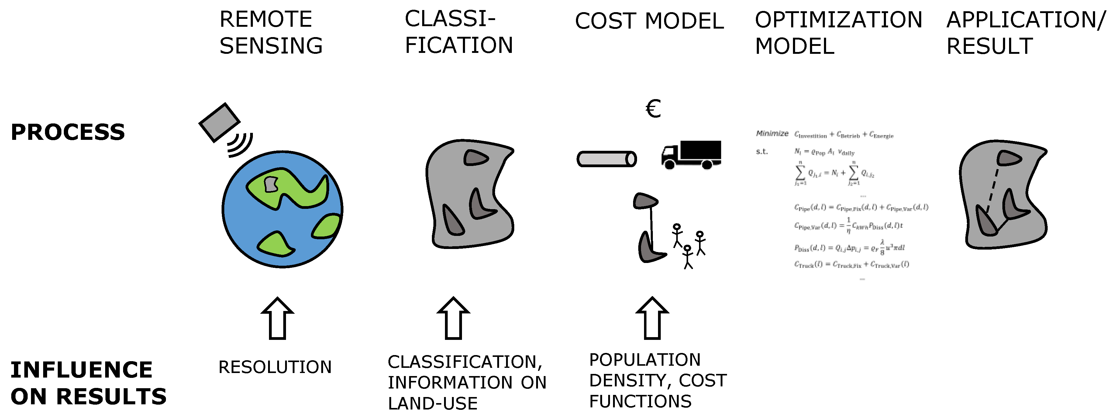
Figure 2.
Slum cluster in Dhaka for 2010 with (right) and without (left) a buffer zone of 10 m, representing a lower spatial resolution.
Figure 2.
Slum cluster in Dhaka for 2010 with (right) and without (left) a buffer zone of 10 m, representing a lower spatial resolution.

Figure 3.
Map of Kibera, Nairobi, from OpenStreetMap (right) compared to Google Maps (left).

Figure 4.
Directed complete graph with four vertices.
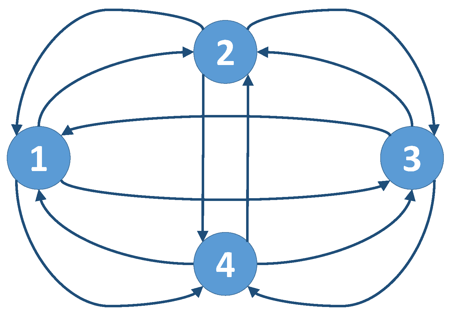
Figure 5.
Composition of the required tank capacity.
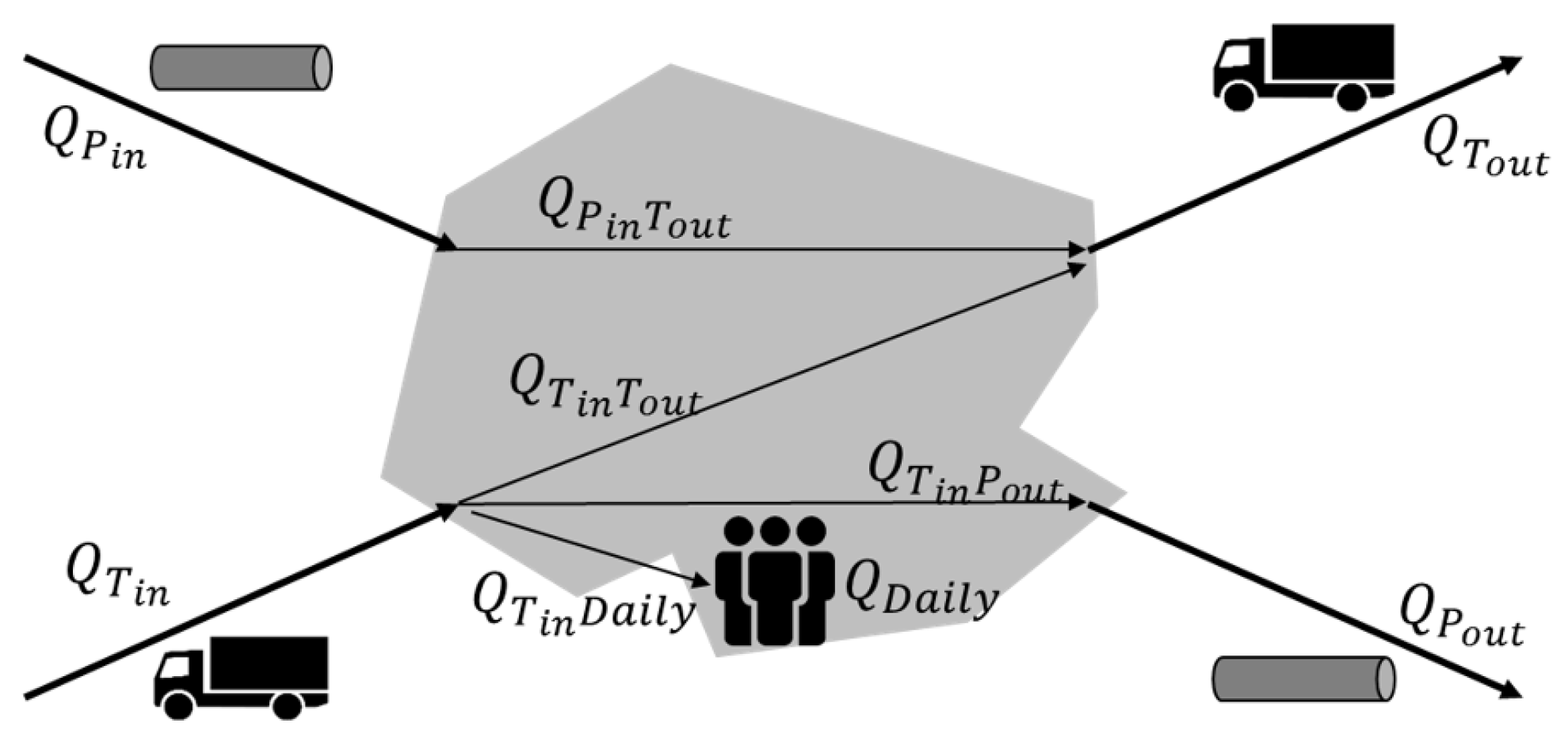
Figure 6.
Decision tree (a) and computational process (b).
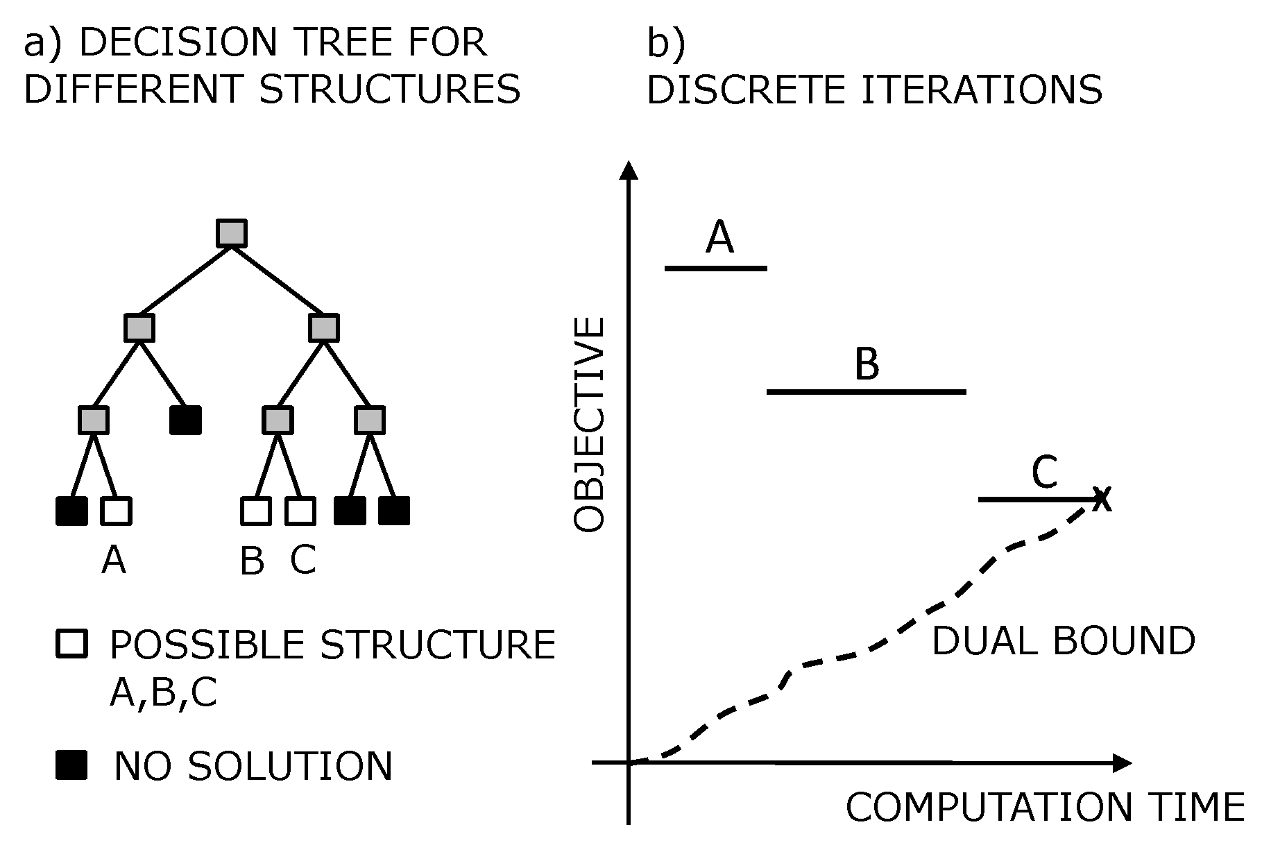
Figure 7.
The seven steps of the TOR approach.

Figure 8.
Optimization result for a slum cluster in Dhaka (2010), Bangladesh.

Figure 9.
Optimization result for a slum cluster in Dar es Salam (2002), Tanzania.

Figure 10.
Optimization result for a slum cluster in Dhaka, Bangladesh, in 2006 (left) and in 2010 (right).
Figure 10.
Optimization result for a slum cluster in Dhaka, Bangladesh, in 2006 (left) and in 2010 (right).

Figure 11.
Optimization result for a slum cluster in Dar es Salam, Tanzania, in 1998 (left) and in 2002 (right).
Figure 11.
Optimization result for a slum cluster in Dar es Salam, Tanzania, in 1998 (left) and in 2002 (right).

Figure 12.
Optimization result for a slum cluster in Dhaka 2010, Bangladesh, with a population density of 100,000 people per km (left) and 50,000 people per km (right).
Figure 12.
Optimization result for a slum cluster in Dhaka 2010, Bangladesh, with a population density of 100,000 people per km (left) and 50,000 people per km (right).
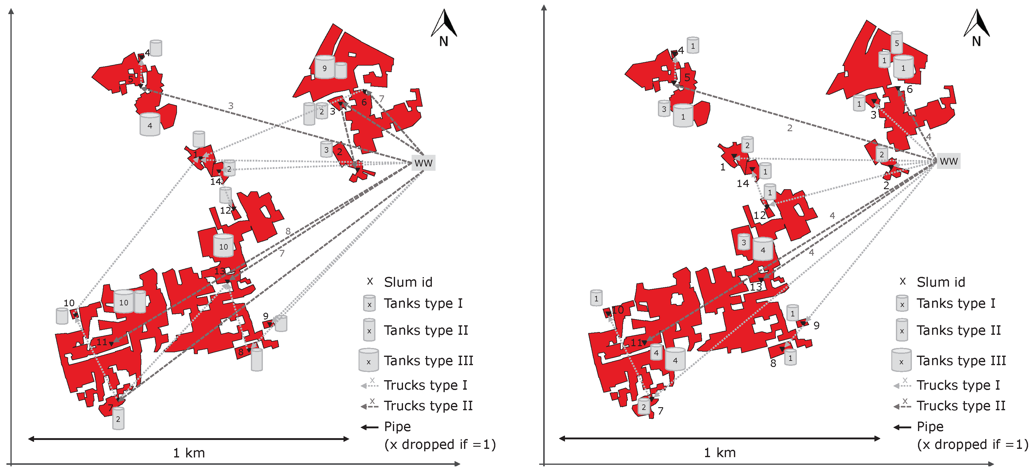
Figure 13.
Optimization result for a slum cluster in Dhaka 2010, Bangladesh, with 14 slums (left) and with low resolution, with a buffer of 10 m (right).
Figure 13.
Optimization result for a slum cluster in Dhaka 2010, Bangladesh, with 14 slums (left) and with low resolution, with a buffer of 10 m (right).

Figure 14.
Optimization result for a slum cluster in Dhaka 2010, Bangladesh, with 14 slums (left) and with additional consideration of geographic barriers (right).
Figure 14.
Optimization result for a slum cluster in Dhaka 2010, Bangladesh, with 14 slums (left) and with additional consideration of geographic barriers (right).
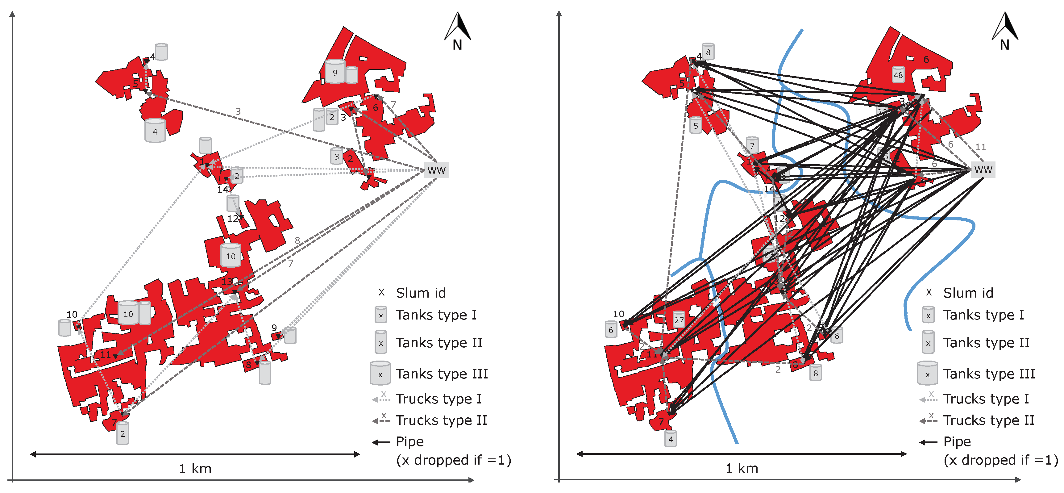
Figure 15.
Optimization result for a slum cluster in Dhaka 2010, Bangladesh, with 14 slums (left) for a cost calculation period of five years and with a period of 15 years (right).
Figure 15.
Optimization result for a slum cluster in Dhaka 2010, Bangladesh, with 14 slums (left) for a cost calculation period of five years and with a period of 15 years (right).
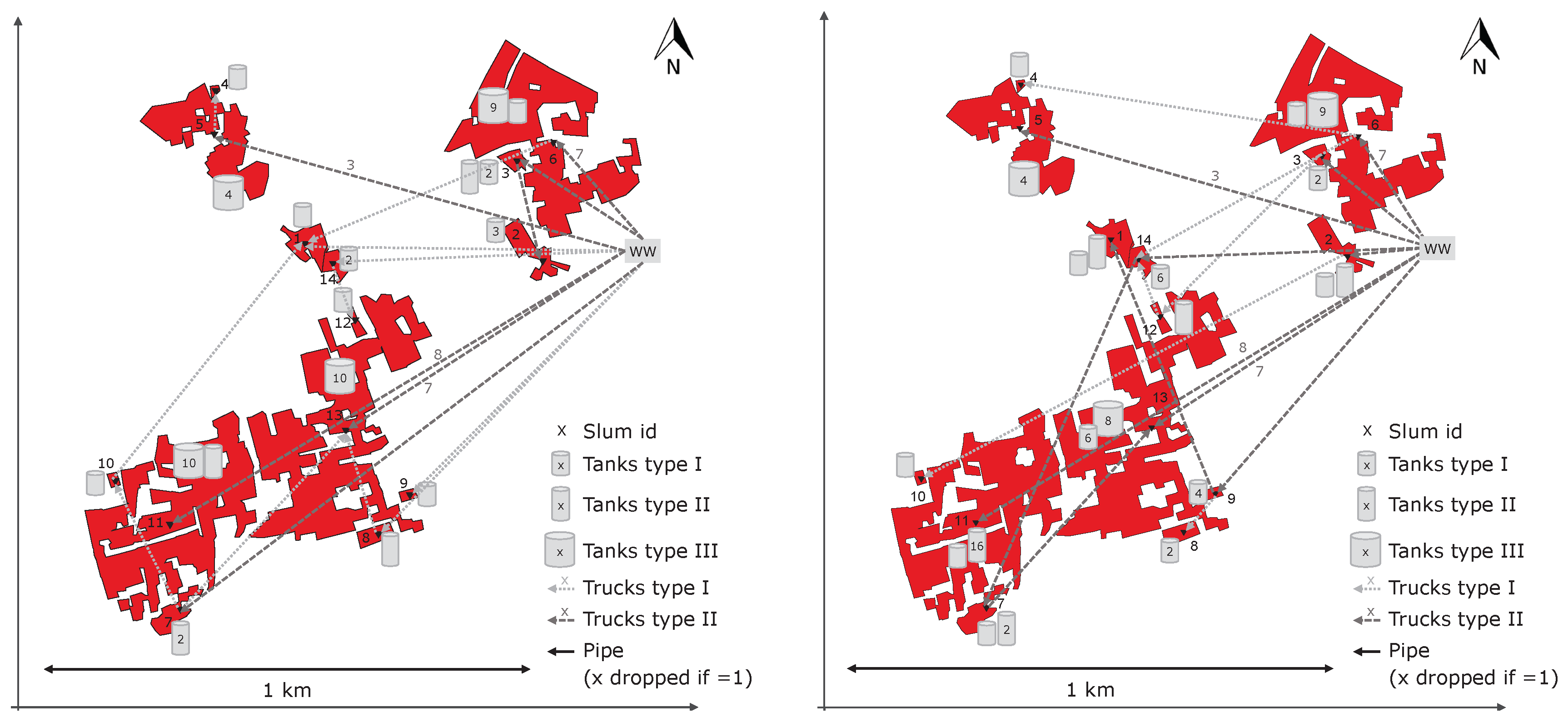
Table 1.
Input parameters for the cost model.
| Parameter | Description | Unit | Parameter | Description | Unit |
|---|---|---|---|---|---|
| Factors from pipe price estimation (in Portugal) | Distance between slums i and j | ||||
| Pump efficiency | Period for calculation | ||||
| Resistance number depending on the diameter of the pipe | Proportion of time of a day in which the pipe is used | ||||
| Factor with which aerial distance between slums is multiplied to estimate route | Factor representing the difference in price level between Portugal and the target country | ||||
| Density of water | Fuel need for truck type k | ||||
| Price of fuel | d | Diameter of pipe | |||
| Typical energy prices | Volume flow on pipe from slum i to j | ||||
| Price for a pump required for a pipe with diameter d | € | Price to buy a truck of type k | € | ||
| Wage of a truck driver | u | flow velocity |
© 2018 by the authors. Licensee MDPI, Basel, Switzerland. This article is an open access article distributed under the terms and conditions of the Creative Commons Attribution (CC BY) license (http://creativecommons.org/licenses/by/4.0/).
Share and Cite
MDPI and ACS Style
Rausch, L.; Friesen, J.; Altherr, L.C.; Meck, M.; Pelz, P.F. A Holistic Concept to Design Optimal Water Supply Infrastructures for Informal Settlements Using Remote Sensing Data. Remote Sens. 2018, 10, 216. https://doi.org/10.3390/rs10020216
AMA Style
Rausch L, Friesen J, Altherr LC, Meck M, Pelz PF. A Holistic Concept to Design Optimal Water Supply Infrastructures for Informal Settlements Using Remote Sensing Data. Remote Sensing. 2018; 10(2):216. https://doi.org/10.3390/rs10020216
Chicago/Turabian StyleRausch, Lea, John Friesen, Lena C. Altherr, Marvin Meck, and Peter F. Pelz. 2018. "A Holistic Concept to Design Optimal Water Supply Infrastructures for Informal Settlements Using Remote Sensing Data" Remote Sensing 10, no. 2: 216. https://doi.org/10.3390/rs10020216
Note that from the first issue of 2016, this journal uses article numbers instead of page numbers. See further details here.