Estimation of Chlorophyll-a Concentration from Optimizing a Semi-Analytical Algorithm in Productive Inland Waters

Abstract

The high nutrient concentrations coming from non-point and point pollution have been linked to algae blooms, especially in hydroelectric plant reservoirs, due to higher residence time compared to rivers. The monitoring of algae is important to prevent risk of contamination by toxins in reservoirs used for drinking water supply. In this context, a physical model-based approach was adopted to retrieve chlorophyll-a (chl a) concentration, a photosynthetic pigment found in all phytoplankton species. We assumed that a semi-analytical algorithm parameterized to a eutrophic reservoir could also be applied to other eutrophic reservoirs, at least the specific inherent optical properties (SIOPs) are not similar. The parameterization was carried out based on Ocean and Land Color Instrument (OLCI) bands aboard Sentinel-3 spacecraft. In our study, the semi-analytical approach showed good performance in retrieving chl a content, with a normalized root mean square error (NRMSE) of 18.7%. The findings encourage the use of a unique semi-analytical algorithm in a reservoir cascade, where the impoundments present similar bio-optical status. The good performance of the algorithm indicates that this approach is rather useful in predicting trophic status in reservoirs.

1. Introduction

Rivers crossing large urban centers in developing countries receive high loads of domestic and industrial wastewater and, when dams are built in polluted stretches, the ecological impact is often severe. The increase in water residence time leads to higher nutrient availability for primary productivity, such as algae blooms. Depending on the type of the phytoplankton assemblage, monitoring water quality is important due to toxins production by some species which are harmful to aquatic life and human health. The consequent pollution lessens the availability of good drinking water for public supply.

All phytoplankton species have the chlorophyll-a (chl a) pigment, widely used as a proxy for the trophic state [1,2,3]. The presence of photoactive pigments in phytoplankton cells enables the detection of algae bloom from space-borne imagery [4]. Due to the interaction of light with different water column constituents, remote sensing has been widely applied in ecological studies [1,5]. The absorption and scattering properties (a and b_b, respectively, referring to

Table 1. Abbreviations and symbols.

Symbols	Definition	Unit
A	Total absorption coefficient, aw + aφ + aCDOM	m−1
aCDOM	Absorption coefficient of colored dissolved organic matter	m−1
aφ	Absorption coefficient of phytoplankton pigment	m−1
aNAP	Absorption coefficient of non-algal particle	m−1
aw	Absorption coefficient of pure water	m−1
bb	Total backscattering coefficient	m−1
bb,p	Backscattering coefficient of particles	m−1
bb,w	Backscattering coefficient of pure water	m−1
Γ	Geometrical factors	sr−1
F	Geometrical light factor	-
Q	Light distribution factor	sr
Rrs	Remote sensing reflectance	sr−1
Chla	Chlorophyll a	mg m−3
CDOM	Colored dissolved organic matter	-
CDM	Colored detrital matter	-
NAP	Non-algal particle	g m−3
AOP	Apparent optical property	-
IOP	Inherent optical property	m−1
S	Spectral slope of aCDOM	nm−1
TSS	Total suspended solids	g m−3
FSS	Fixed suspended solids	g m−3
VSS	Volatile suspended solids	g m−3
u	Ratio of backscattering coefficient to the sum of absorption and backscattering coefficient	-
Y	Spectral power of bbp	-

for abbreviations and symbols) of some pigments such as chl a, and chlorophyll b (chl b), carotenoids and phycobilins [6], are responsible for modeling radiometric quantities such as remote sensing reflectance (R_rs, in sr⁻¹) [7]. R_rs is an apparent optical property, i.e., it depends on the properties of the water column and underwater light field geometry [8]. Based on this optical relationship, semi-analytical algorithms have been proposed for retrieving optically significant constituents (OSCs) [1,9,10,11,12,13,14], bathymetry [15] and Secchi disk depth, Z_SD [16]. This approach considers R_rs as a function of a and b_b for each OSC (phytoplankton pigments, detritus and dissolved organic matter), where a and b_b are linear combinations between specific absorption and backscattering coefficients (a^* and b_b^*, respectively) of each OSC times its concentration [17].

Semi-analytical algorithms are simplified solutions to the radiative transfer equation [4,18]. In other words, they model the underwater light behavior based on physical principles represented by spectral measurements of a and b_b as well as factors of light geometry. In the model presented by Gordon et al. (1988), all the parameters are spectral, with the exception of OSC concentration; therefore, measurements of R_rs, a and b_b can be represented by a spectral band set. Hyperspectral data, such as AVIRIS airborne [19], Hyperion EO-1 sensor [1] and CASI [15], have already used in this sort of modeling. Indeed, the performance of the semi-analytical algorithm is closely associated with wavelengths adopted in adjustment. According to this statement, a spectral solution must be applied to solve the inversion problem of the model and derive the OSC concentrations [1,9,19,20]. These inversion methods are numerical optimization techniques, in which the values of the variables or concentrations are changed to each iteration in order to reduce the difference between calculated and measured R_rs spectra [1].

Nevertheless, parameterizing semi-analytical algorithms is a challenge, since the model might represent a large bio-optical variability of a water body and the performance of a semi-analytical algorithm is closely linked to its bio-optical parameters based on the quality of the specific inherent optical properties (SIOPs), i.e., a^* and b_b^* of each OSC [18]. SIOPs depend upon the sort of OSC, independent of its concentration [8]. In a reservoir cascade, the bio-optical variation can be large due to the filtration process upstream to downstream, improving the water quality. Therefore, the SIOPs can be smooth along the cascade system caused by the cascading reservoir continuum process [21]. However, although the trophic level improves, it is expected that there is similarity in phytoplankton assemblages between adjacent reservoirs.

In this context, we assumed that a semi-analytical chl a predicting algorithm parameterized for a eutrophic reservoir could be applied to estimate the content of this pigment in other eutrophic reservoirs with similar bio-optical status. Therefore, this study aimed to design an accurate semi-analytical algorithm for chl a retrieval in productive inland waters. In situ bio-optical measurements were collected to parameterize the algorithm. The specific objectives were: (a) to analyze the bio-optical status of two eutrophic reservoirs; (b) to investigate the potential of bands from Ocean and Land Colour Instrument (OLCI) Sentinel-3 satellite for predicting chl a concentration; (c) to simulate R_rs in order to determine light geometry factors; (d) to test different datasets to calibrate the semi-analytical algorithm and (e) to discuss the limitations and potentials for long-term monitoring.

Although hyperspectral data are often used to parameterize semi-analytical algorithms [1,15,19], we will use representative multispectral bands of absorption and scattering features related to OSCs. In this context, bands from the OLCI, onboard Sentinel-3 spacecraft (ESA, https://sentinel.esa.int/web/sentinel/missions/sentinel-3), will be tested to estimate OSC concentration.

The newly parameterized semi-analytical algorithm was based on the relationship between reflectance data and IOP measurements as proposed by [7]. In this research, we adopted above water surface R_rs measurements and in situ IOPs to parameterize and calibrate the semi-analytical algorithms. Three different parameterizations were tested taking into account two seasonally different datasets and a mixture of both datasets. These datasets were collected in a highly productive reservoir (chl a higher than 700 mg m⁻³). The validation of the semi-analytical algorithms was done from data measured in a downstream eutrophic reservoir. The outcomes were satisfactory, encouraging the parameterization of semi-analytical algorithms for estimating chl a content in similar aquatic ecosystems. This sort of methodology can also be useful in estimating the trophic status in other reservoirs.

2. Materials and Methods

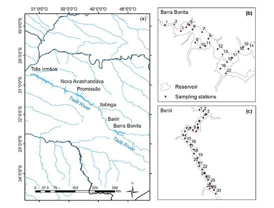
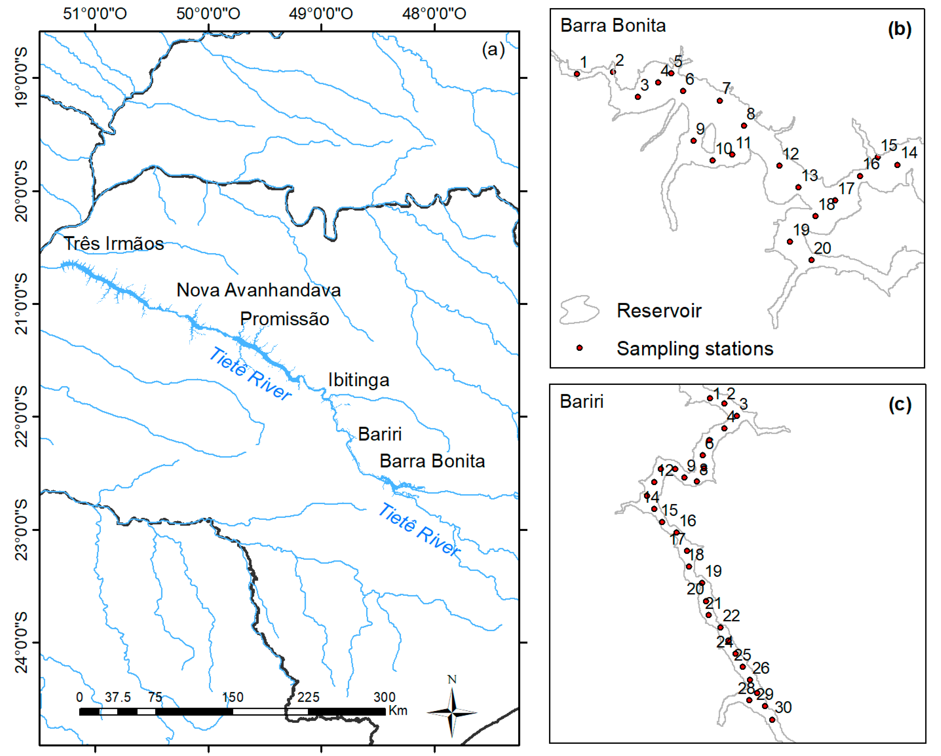
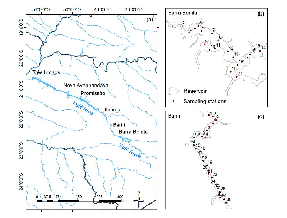
2.1. Study Area and Sampling

The study was carried out in two eutrophic reservoirs, Barra Bonita (BB) and Bariri (BA), both located in the middle basin of the Tietê River, São Paulo State, Brazil (Figure 1). They are the first and second reservoirs in the low and middle course of the Tietê River, and close to point sources of wastewater discharge in big urban centers. The high trophic level associated with anthropic tasks leads to algal blooms in these reservoirs, especially cyanobacteria dominating the phytoplankton community [2,21,22], although variations in phytoplankton species are closely linked to water column mixing events and residence time [23].

Originally built for electrical power generation, BB hydroelectric plant has been operational since 1963, and its reservoir has multiple uses such as fishing, waterway transport and recreation among others. BB is a storage reservoir and the first of six reservoirs cascading in the Tietê River, with a flood area of 310 km², a volume of 3.622 × 10⁶ m³ and an average depth of 10 m. The variation of quota ranges from 439.5 m to 451.5 m (AES Tietê, Arlington, USA; www.aestiete.com.br), while the retention time varies from 30 days (austral summer) to 180 days (austral winter). The control of water flow leads to a range of 200 m³ s⁻¹ in the dry season (May–October) to 1500 m³ s⁻¹ in the wet season (November–April) [24]. BB is a polymictic reservoir, i.e., with the occurrence of thermal stratification. The high nutrient load associated with cold fronts leads to blooms of cyanobacteria in the summer and diatoms in the winter [25]. Studies have shown that the high trophic level leads to greenhouse gas emission from this reservoir [26].

In turn, BA is the second reservoir in the cascade of the Tietê River, with the smaller area of 63 km², volume of 607 × 10⁶ m³ and the quota variation ranges from 426.5 to 427.5 m. It has been operational since 1965 (AES Tietê). BA is run-of-river reservoir, with an average depth of about 9 m and produces electrical power in periods of high water flow [21]. The residence time is less in BA, ranging from 7 to 24 days [21]. BA also presents a high trophic status, whose phytoplankton assemblage is dominated by cyanobacteria [21].

Calibration and validation datasets were gathered in three field campaigns, conducted in BB, on 5–9 May (labeled BB1) and 13–16 October 2014 (labeled BB2), and in BA, on 15–18 August 2016. The data were collected from sampling stations selected according to variation of the water color [27]. Such sampling design built to reservoirs provides the maximum optical variability in collected samples. Water samples and radiometric data were collected in the three field campaigns. The water samples were carefully stored and filtered for later laboratorial analysis for determination of OSC concentration and absorption coefficient. In turn, the radiometric data were used to compute the R_rs spectra. The datasets collected in 2014 were used to parameterize and calibrate the semi-analytical algorithm, while validation was done using the 2016 dataset.

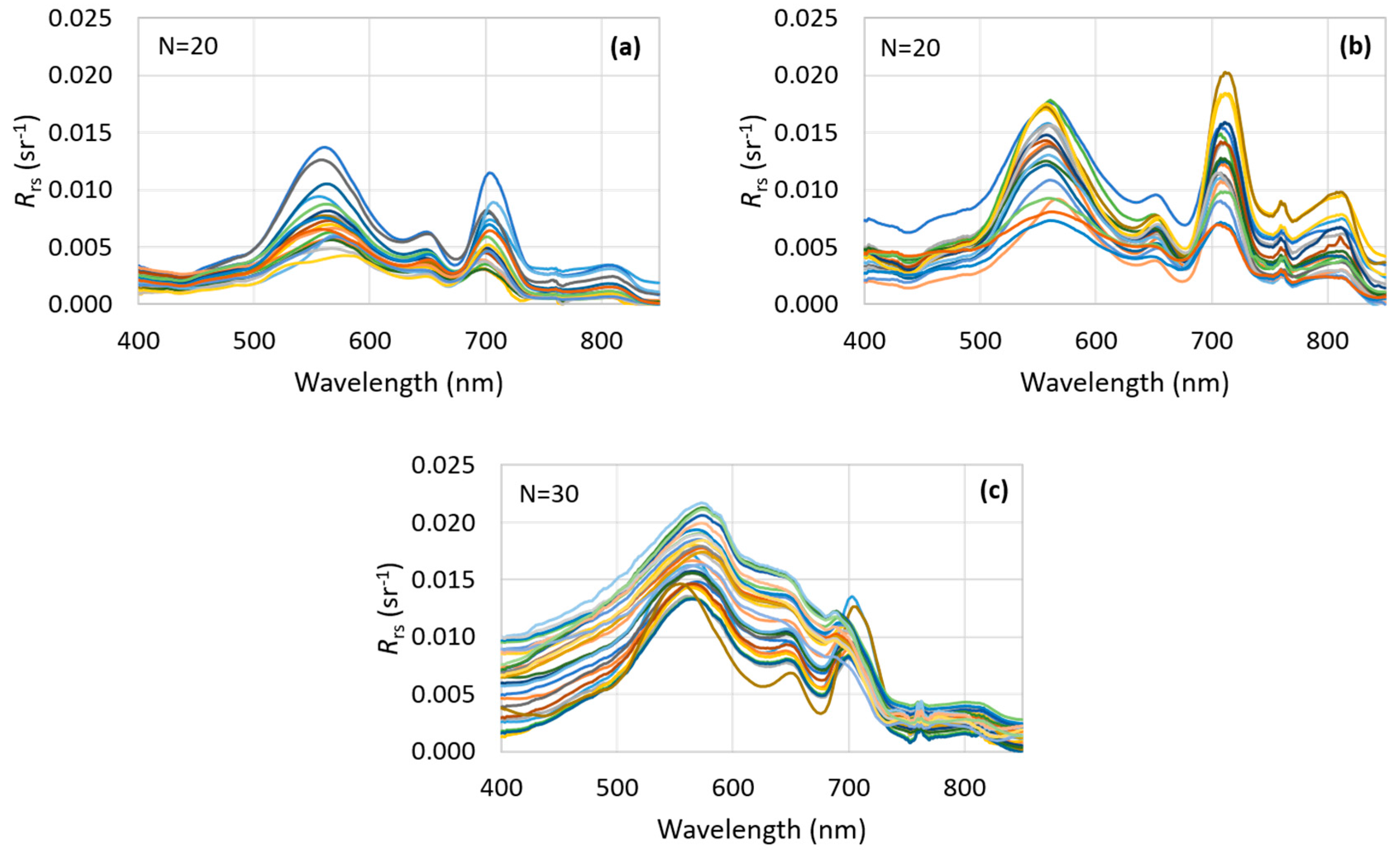
2.2. Remote Sensing Reflectance, R_rs

Above-surface R_rs was calculated from radiometric measurements acquired in situ. Three RAMSES spectroradiometers (TriOS, Rastade, Germany) were used. Two ARC sensors were used to measure sky radiance (L_sky, in W m⁻² sr⁻¹) and total radiance (L_t, in W m⁻² sr⁻¹), composed of water-leaving radiance (L_w, in W m⁻² sr⁻¹) and surface-reflected radiance (L_r, in W m⁻² sr⁻¹); and one cosine collector (ACC/RAMSES) to acquire downwelling irradiance just above the surface (E_s, in W m⁻²). To avoid boat shading, the sensors were oriented at right angles to the Sun’s azimuthal plane. Additionally, one radiometer was pointed at 40° in relation to the nadir plane to measure L_t, while a second sensor was pointed at 40° to the zenith plane to measure L_sky. To take E_s, the cosine collector was oriented to the zenith. This acquisition geometry was adopted in order to minimize surface-reflected light [28] using the method proposed by [29] which was applied to calculate the R_rs, as shown in Equation (1).

$$R_{\mathrm{rs}}\left(\lambda ,\theta ,\phi \right)\approx T_{\mathrm{rs}}\left(\lambda ,\theta ,\phi \right)-F\left(\lambda ,\theta ,\phi \right) S_{\mathrm{rs}}\left(\lambda ,{\theta }^{\prime },\phi \right)-\mathsf{\Delta }\left(\theta ,\phi \right),$$

(1)

where T_rs is the total remote sensing reflectance (ratio of L_t to E_s); S_rs is the sky remote sensing reflectance ratio of L_sky to E_s); F is the Fresnel reflectance of the water surface, depending on a given angular geometry; and Δ is a bias (spectrally constant value). According to [29], Δ can be estimated by assuming R_rs(750) as 0 sr⁻¹ in ocean waters, whereas in coastal turbid water Δ can be fitted by comparing a modeled spectral R_rs with a spectral R_rs derived from Equation (1). Modeled spectral R_rs can be modeled as a function of a(λ) and b_b(λ), as indicated in Equation (2).

$$R_{\mathrm{rs}}\left(\lambda ,\theta ,\phi \right)\approx F\left(a\left(\lambda \right),b_{\mathrm{b}}\left(\lambda \right),\theta ,\phi \right),$$

(2)

where a(λ) and b_b(λ) can be modeled from bio-optical models, taking into account each OSC (phytoplankton pigment, NAP and CDOM).

2.3. Laboratory Measurements

2.3.1. OSC Concentration

The water samples collected were used to determine the concentrations of chl a and suspended matter. After each day of collection, the water samples were filtered through a GF/F Whatman glass fiber filter, with 0.7 µm pore size and 47 mm diameter (GE Healthcare, Little Chalfont, UK). To measure the chl a concentration the method of [30] was adopted using chl a extraction via a 90% acetone solution. Chl a estimation was done from absorbance measurements taken at 663 and 750 nm with a spectrophotometer, using a quartz cuvette of 1 cm. In turn, the concentrations of total, fixed and volatile suspended solids (TSS, FSS and VSS, respectively) were determined using the 2540 Solids methods from APHA [31].

2.3.2. Absorption Coefficients

To measure the absorption coefficient of the particles (a_p), phytoplankton (a_φ), non-algal particles (a_NAP) and colored dissolved organic matter (a_CDOM) water samples were collected in situ, filtered on the day of collection, and suitably stored until analysis. For each sampling station, a_p, a_φ and a_NAP measurements require a simple filtration on a GF/F Whatman glass fiber filter (GE Healthcare, Little Chalfont, UK). The filter with retained particles was stored in the dark, frozen and in a jar to prevent decomposition of the material. For a_CDOM, the water filtered through a GF/F filter was refiltered on nylon membrane or polycarbonate filter (GE Healthcare, Little Chalfont, UK), with 0.2 µm pore size and 47 mm diameter. The refiltered water was stored in a jar at 4 °C in the dark.

In the laboratory, a_p, a_φ and a_NAP were measured using the ‘Transmittance-Reflectance’ method proposed by [32,33,34]. The readings were taken using a UV-VIS 2600 spectrophotometer (Shimadzu, Kyoto, Japan), with dual beam and integrating sphere mode. To convert measurements into specific absorption coefficient (a^*), a_p, a_φ and a_NAP were divided by their respective concentration. In turn, a_CDOM was measured adopting Bricaud et al.’s [35] method, using a UV-VIS 2600 spectrophotometer, with single beam (Shimadzu, Kyoto, Japan). The same spectral range of 280–800 nm and 1 nm spectral resolution were used. Ultra-pure water was adopted as blank reference.

2.4. Parameterization of the Semi-Analytical Algorithm

Semi-analytical algorithms are simplified solutions from the radiative transfer equation (RTE), which involves relationships between inherent and apparent optical properties [4,7], as shown in Equation (3) [7].

$$R_{\mathrm{rs}}=\gamma \frac{b_{\mathrm{b}}}{a+b_{\mathrm{b}}},$$

(3)

where the ratio of b_b for the sum of a and b_b can be expressed by u (Equation (4)).

$$u=\frac{b_{\mathrm{b}}}{a+b_{\mathrm{b}}},$$

(4)

This approach has been utilized to estimate the different OSCs simultaneously [1,5,36]. This kind of modeling enables retrieval of the concentrations of OSCs because a and b_b may be decomposed in terms of specific absorption and backscattering coefficient (a_j^* and b_bj^*, respectively) of each OSC, j, and their concentrations, C_j, as shown in Equations (5) and (6), respectively [1,7].

$$a=a_{\mathrm{w}}+{\displaystyle \sum }_{j=1}^n{a_{\mathrm{j}}}^{*}·C_{\mathrm{j}}=a_{\mathrm{w}}+a_{\mathsf{\varphi }}+a_{\mathrm{CDOM}}+a_{\mathrm{NAP}}$$

(5)

$$b_{\mathrm{b}}=b_{\mathrm{bw}}+{\displaystyle \sum }_{j=1}^n{b_{\mathrm{bj}}}^{*}·C_j=b_{\mathrm{bw}}+b_{\mathrm{bp}}$$

(6)

where a_w is the absorption of pure water, and b_bw is the backscattering of pure water, both of them determined by [37]. Taking into account Equations (5) and (6), it is possible to derive water column properties from known R_rs spectra [1,19]. In other words, R_rs can be expressed as a function of the different OSCs in the water column (Equation (7)).

$$R_{\mathrm{rs}}\left(\lambda \right)=F\left(a_{\mathrm{w}}\left(\lambda \right),b_{\mathrm{bw}}\left(\lambda \right),a_{\mathsf{\varphi }}\left(\lambda \right),a_{\mathrm{NAP}}\left(\lambda \right),a_{\mathrm{CDOM}}\left(\lambda \right),b_{\mathrm{bp}}\left(\lambda \right)\right)$$

(7)

Thus, an algorithm is parameterized based on measurements of SIOPs (a_j^* and b_bj^*) and geometrical relations of light field (γ) [1,9,20]. Spectra of SIOPs might be fixed in the model from average spectral measures obtained in the laboratory, while γ is a fixed value for every wavelength. R_rs spectra are obtained for each sampling station. Consequently, the concentration of OSCs becomes the variable to be estimated. It can be seen that this semi-analytical algorithm is spectral, where the values of OSC concentration are derived to fit the R_rs spectrum. In the Matrix Inversion Method (MIM), the semi-analytical algorithm is represented as an M × N matrix, where M is the number of bands and N is the number of OSC [1,9]. Due to the mathematical complexity of those models, it is needed to use numerical optimization techniques, which often use an iterative process aiming to minimize the error produced by the model.

It is therefore desirable to use hyperspectral data [1,19], which represent different spectral features relating to each OSC in the water column. Despite that, there are data of multispectral sensors with specific bands for applications in remote sensing of the water color, such as MERIS, OLCI, SeaWiFS, among others. In this study, we tested the potential of OLCI Sentinel-3 bands in retrieving the chl a content from a semi-analytical algorithm.

Three different parameterizations of the semi-analytical algorithm were tested considering: (i) mean values of SIOPs collected in BB1 (austral autumn); (ii) mean values of SIOPs collected in BB2 (austral spring); and (iii) mean values of SIOPs collected in BB1 and BB2.

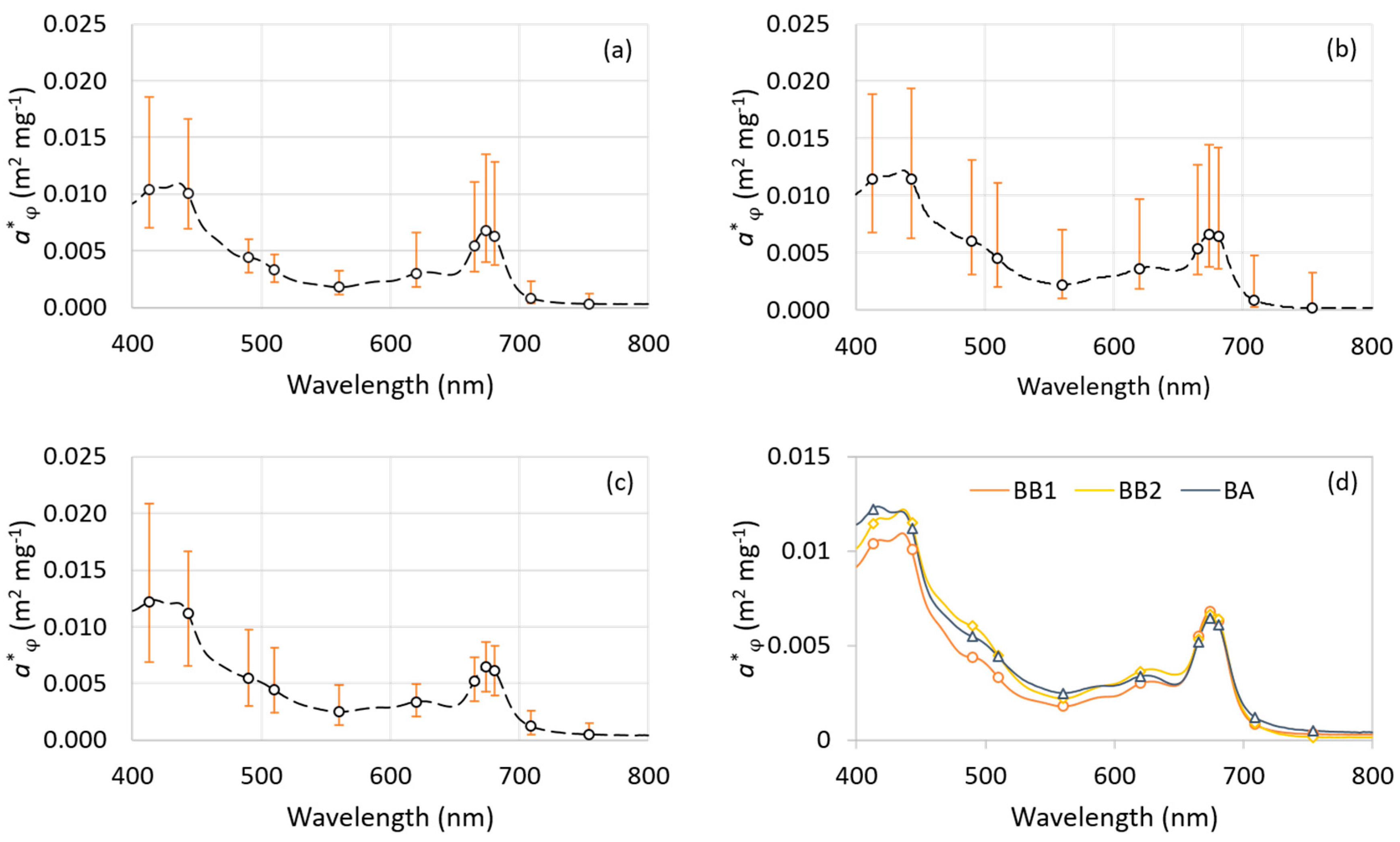
2.4.1. Estimation of SIOPs

To parameterize the semi-analytical model (Equations (8)–(10)), we have defined a^* for each OSC. a^*_φ and a^*_NAP were determined by using bio-optical measurements obtained from laboratory analysis. Average values of a^*_φ and a^*_NAP were adopted as input in the semi-analytical model. In turn, b_bp and b_bw were defined by Equation (10) and proposed by [37], respectively.

The a^*_φ(λ) was defined from the ratio of a_φ(λ) to chl a concentration, [chl a], as displayed in Equation (8). The transmittance-reflectance method was adopted to determine a_φ(λ) in the laboratory [32,33,34], while chl a content was defined by acetone through the extraction method (Golterman 1978), as detailed in Section 2.3.

$${a^{*}}_{\mathsf{\varphi }}\left(\lambda \right)=\frac{a_{\mathsf{\varphi }}\left(\lambda \right)}{\left[\mathrm{chl} a\right]}$$

(8)

In turn, a^*_NAP was estimated from the ratio of a_NAP to the concentration of FSS, [FSS] (Equation (9)). Section 2.3 shows the methods used to determine a_NAP [Tassan and Ferrari 1995, 1998, 2002] and the content of FSS [31] in the laboratory.

$${a^{*}}_{\mathrm{NAP}}\left(\lambda \right)=\frac{a_{\mathrm{NAP}}\left(\lambda \right)}{\left[\mathrm{FSS}\right]}$$

(9)

a_CDOM was analytically retrieved by assuming the relationship proposed by [35], as shown in Equation (10).

$$a_{\mathrm{CDOM}}\left(\lambda \right)={a^{*}}_{\mathrm{CDOM}}\left(440\right)·e^{\left(-S\left(440-\lambda \right)\right)}$$

(10)

where a^*_CDOM(440) = 1; S is the spectral slope of a_CDOM. We assumed an average value of S of 0.015 nm⁻¹ for all stations [4,18,35,38].

b_bp(λ) was analytically derived from Smith and Baker’s method [37], as shown in Equation (11).

$$b_{\mathrm{bp}}\left(\lambda \right)=b_{\mathrm{bp}}\left(560\right)·{\left(\frac{560}{\lambda }\right)}^Y$$

(11)

where Y is the spectral power of b_bp and λ is the wavelength. Values of b_bp(560) were obtained from the inversion of the semi-analytical model. The spectral power of b_bp(Y) was modeled from Equation (12) [39], used by [22] in a quasi-analytical algorithm (QAA) applied to the BB reservoir.

$$Y=2.0\left\{1-1.2 exp\left(-0.9\frac{r_{\mathrm{rs}}\left(443\right)}{r_{\mathrm{rs}}\left(560\right)}\right)\right\}$$

(12)

Equation (13) shows the formula of the semi-analytical algorithm parameterized in this research to estimate R_rs, taking into account a_w and b_bw determined by [37]. The other IOPs of the equation were defined as in Equations (8)–(10) and in turn, R_rs are those measurements in situ.

$$R_{\mathrm{rs}}=\gamma \frac{b_{\mathrm{bw}}+b_{\mathrm{bp}}}{a_{\mathrm{w}}+{a^{*}}_{\mathsf{\varphi }}·\left[\mathrm{chl}a\right]+{a^{*}}_{\mathrm{NAP}}·\left[\mathrm{FSS}\right]+a_{\mathrm{CDOM}}+b_{\mathrm{bw}}+b_{\mathrm{bp}}}$$

(13)

From the inversion of Equation (13) we estimated [chl a], [FSS], a^*_CDOM(440) and b_b(560) simultaneously.

All the model parameters are spectrally dependent, with the exceptions of the γ and OSC concentrations (chl a and FSS) which are the variables to be retrieved. The spectral dependence is an advantage of the semi-analytical algorithms, because several wavelengths can be used in a single model simultaneously in order to estimate different OSCs simultaneously as well [19,29]. With known R_rs measurements acquired in situ at n channels, the semi-analytical algorithm can be expressed as (Equation (14)):

$$\begin{gathered} R_{\mathrm{rs}}\left({\lambda }_1\right)=F\left(a_{\mathrm{w}}\left({\lambda }_1\right),b_{\mathrm{bw}}\left({\lambda }_1\right),a_{\mathsf{\varphi }}\left({\lambda }_1\right),a_{\mathrm{NAP}}\left({\lambda }_1\right),a_{\mathrm{CDOM}}\left({\lambda }_1\right),b_{\mathrm{bp}}\left({\lambda }_1\right)\right) \\ {R}_{\mathrm{rs}}\left({\lambda }_2\right)=F\left(a_{\mathrm{w}}\left({\lambda }_2\right),b_{\mathrm{bw}}\left({\lambda }_2\right),a_{\mathsf{\varphi }}\left({\lambda }_2\right),a_{\mathrm{NAP}}\left({\lambda }_2\right),a_{\mathrm{CDOM}}\left({\lambda }_2\right),b_{\mathrm{bp}}\left({\lambda }_2\right)\right) \\ ⋮ \\ {R}_{\mathrm{rs}}\left({\lambda }_n\right)=F\left(a_{\mathrm{w}}\left({\lambda }_n\right),b_{\mathrm{bw}}\left({\lambda }_n\right),a_{\mathsf{\varphi }}\left({\lambda }_n\right),a_{\mathrm{NAP}}\left({\lambda }_n\right),a_{\mathrm{CDOM}}\left({\lambda }_n\right),b_{\mathrm{bp}}\left({\lambda }_n\right)\right) \end{gathered}$$

(14)

where n is the number of channels used in the parameterization of the algorithm to represent the spectra of AOPs and IOPs.

The better the spectral representation of the algorithm, the more accurate the estimation of concentrations will be. Lee et al. [19] used hyperspectral data from AVIRIS aircraft to derive properties of the water column and bottom, while Brando and Dekker [1] adopted bands from the Hyperion EO-1 sensor to estimate chl a, tripton and CDOM concentrations.

In this context, our semi-analytical algorithm was parameterized based on OLCI Sentinel-3 bands. We parameterized the model from SIOPs spectral measurements determined in the laboratory considering wavelengths from the OLCI Sentinel-3 sensor. Therefore, the factor associated with the light geometry might still be estimated.

2.4.2. Factors of Light Geometry

Further, the factor of light geometry, γ, associated with the factors of light field (f) and light distribution (Q), were determined based on Equation (3) and spectral measurements of R_rs and IOPs (a and b_b), both simulated using Hydrolight software [40]. The simulation was carried out considering a content of chl a from 10 to 1000 mg m⁻³, varying every 10 mg m⁻³ from 10 to 100 mg m⁻³ and every 25 mg m⁻³ from 100 to 1000 mg m⁻³, totaling 45 simulations. A gain value, i.e., γ or f/Q, was fitted between the average spectra of simulated R_rs (from Equation (3)) and u (ratio of b_b to sum of a and b_b) based on the model proposed by [7]. In this way, the γ value becomes the variable to be determined by the model. The γ value was retrieved using a numerical optimization method and adopted in the parameterized semi-analytical algorithm.

2.4.3. Inversion of the Semi-Analytical Algorithm

To solve the semi-analytical algorithm and retrieve the concentrations of OSCs we need to apply an inversion method. In general, these inversion methods are numerical optimization techniques, in which the values of the variables (concentrations) are changed to each iteration to minimize the difference between calculated and measured R_rs spectra [1]. In other words, the chl a concentrations are retrieved from an iterative fit of the semi-analytical algorithm.

The parameterization of the semi-analytical algorithm is therefore based on spectral measurements. For that reason, there is the need to use imagery from sensors with spectral bands representative of the OSCs. In this context, we chose to evaluate the potential of OLCI Sentinel-3 bands for 11 channels centered at 412.5, 442.5, 490, 510, 560, 620, 665, 673.75, 681.25, 708.75 and 753.75 nm [41]. These eleven OLCI Sentinel-3 bands were simultaneously used to represent the R_rs spectrum. The OLCI sensor was designed for application in water bodies, with bands located in absorption features of phytoplankton pigments. There are three spectral bands (665, 673.75 and 681.25 nm) associated with absorption and fluorescence by chl a in the region of the red alone. Other bands widely used in modeling chl a are also available in OLCI Sentinel-3, such as 442.5, 708.75 and 753.75 nm. Another important band for remote sensing of harmful algal bloom is 620 nm, where the absorption feature of phycocyanin pigment is associated with cyanobacteria [42,43].

There are different numerical optimization methods to invert the semi-analytical model, such as MIM [9], the Garver-Siegel-Maritorena model—GSM [10], neural network [44], and least squares [45]. In this work, the adjustment of OSC concentrations was undertaken using GRG2 (Nonlinear Generalized Reduced Gradient), a method of numerical optimization based on a nonlinear generalized reduced gradient. GRG2 is an iterative process aiming at finding the best fit based on minimum error produced by the model. In this research, our stop criterion was the root mean square error (RMSE). We chose to use the GRG2 method due to its easy applicability in in situ measurements. In addition, the advantages of these nonlinear approaches compared to some linear techniques are the reduction of the execution time and more reliable results. This method is implemented in the SOLVER tool, available in Excel Microsoft Office software.

2.5. Assessment of the Semi-Analytical Algorithm

To evaluate the inversion of the parameterized bio-optical model, the following statistical metrics were used: RMSE (Equation (15)), normalized root mean square error (NRMSE, Equation (16)), mean absolute percentage error (MAPE, Equation (17)), slope and bias (Equation (18)).

$$\mathrm{RMSE}= \sqrt{\frac{1}{n}{\displaystyle \sum }_i^n{\left(x_{\mathrm{est},\mathrm{i}}-x_{\mathrm{meas},\mathrm{i}}\right)}^2}$$

(15)

$$\mathrm{NRMSE}= \frac{RMSE}{x_{\mathrm{meas},\max }-x_{\mathrm{meas},\min }}\times 100\%$$

(16)

$$\mathrm{MAPE}=\frac{1}{n}{\displaystyle \sum }_i^n\left(\left|\frac{x_{\mathrm{est},\mathrm{i}}-x_{\mathrm{meas},\mathrm{i}}}{x_{\mathrm{meas},\mathrm{i}}}\right|\right)\times 100\%$$

(17)

$$bias=\frac{1}{n}{\displaystyle \sum }_i^n\left(x_{\mathrm{est},\mathrm{i}}-x_{\mathrm{meas},\mathrm{i}}\right)$$

(18)

where x_est,i and x_meas,i are estimated and measured values of chl a concentration. These statistics metrics enable evaluation of the optical closure between estimated and measured R_rs spectra. The fitting was assessed in terms of individual wavelength and each sampling station.

3. Results

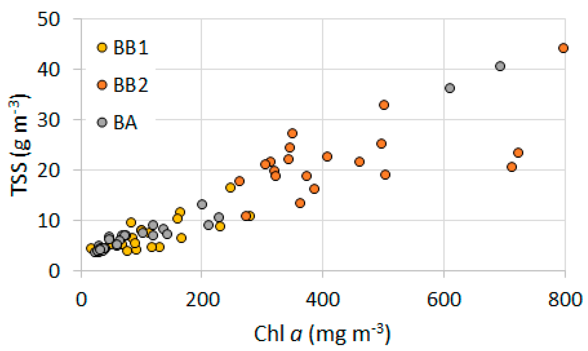
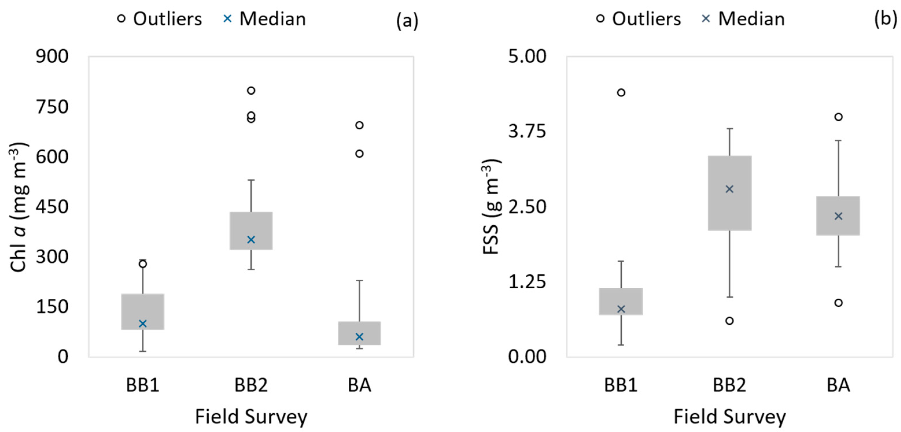
3.1. Water Quality Characterization

Table 2. Statistical description of water quality parameters: chl a (mg m⁻³), total suspended solids (TSS), (g m⁻³), chl a: TSS (mg g⁻¹) and Z_SD (m).

Field	Statistic	Chl a	TSS	Chl a: TSS	ZSD
BB1	Av (SD)	119.8 (73.0)	7.1 (3.4)	16.6 (6.9)	1.5 (0.5)
	Min-Max	17.7–279.9	3.6–16.3	4.0–27.9	0.8–2.3
BB2	Av (SD)	406.2 (137.1)	20.7 (5.0)	20.3 (6.8)	0.6 (0.1)
	Min-Max	263.2–797.8	10.8–32.8	12.9–35.0	0.37–0.78
BA	Av (SD)	117.12 (156.4)	8.3 (8.4)	12.1 (4.7)	1.2 (0.3)
	Min-Max	25.1–694.3	3.6–40.3	6.3–23.9	0.5–1.6

shows the water quality parameters for the BB1, BB2 and BA surveys. BB2 clearly showed the highest chl a concentration with an average value of 406.2 mg m⁻³, whereas chl a content behavior was statistically similar for both BB1 and BA (average chl a content of 119.8 mg m⁻³ and 117.12 mg m⁻³, respectively). The mean TSS concentration was much higher in BB2, with a mean value of 20.7 g m⁻³, whilst BB1 and BA exhibited similar values (7.1 g m⁻³ and 8.3 g m⁻³, respectively). Despite that, the maximum value was reported in BA, with 40.3 g m⁻³, indicating a high contribution of non-algal particles in TSS. This address can be confirmed by the chl a: TSS ratio. The higher the chl a: TSS value, the higher the contribution of the phytoplankton biomass to TSS. Therefore, the highest contribution of phytoplankton was registered in BB2, with a mean chl a: TSS of 20.3 mg g⁻¹. BB1 also showed a high value of chl a: TSS (16.6 mg g⁻¹), while BA exhibited the lowest ratio (12.1 mg g⁻¹).

In terms of their bio-optical constituents, both BB1 and BB2 exhibited higher complexity than BA. In general, the lower the correlation among the different OSCs, the higher the bio-optical complexity. BB1 and BB2 displayed a correlation coefficient between chl a and TSS of 0.75 and 0.60, respectively, while BA showed a correlation coefficient of 0.99. This high value indicates that TSS is strongly associated with the phytoplankton biomass in BA, whereas allochthon sources of TSS coming from drainage basin is small compared to autochthonous sources, i.e., primary production. Figure 2 shows the scatterplot between chl a and TSS for every field survey that addresses the higher correlation found in BA.

Figure 3 shows the boxplots for chl a and FSS concentrations gathered in each field survey. It can be seen that although extremely high chl a values have been measured, most were regarded as outliers. Furthermore, sampling station 3 in BB2 (with a maximum chl a content of 797.8 mg m⁻³) was not adopted in parameterizing the semi-analytical algorithm because there were measurements of a_NAP. Therefore, the maximum chl a value used in parameterization was 723.5 mg m⁻³. When analyzing OCSs, the main difference between BB1 and BA related to sediment concentrations. Inorganic portion is rather lower in BB1 than in the other two field surveys. From this result, it is expected that a semi-analytical algorithm parameterized with the BB2 dataset will have a better performance than that parameterized with the BB1 dataset to applications in BA.

These variations in chl a and FSS directly affect the R_rs curves measured in each field survey. High chl a concentrations lead to highlight absorption features of phytoplankton pigment, while high FSS concentrations tend to increase the reflectance in every visible region. Due to the spectral nature of the semi-analytical algorithm, R_rs and SIOP shapes are strongly associated with its performance.

3.2. Optical Properties

Figure 4 shows the R_rs spectra acquired in situ in May (Figure 4a) and October 2014 (Figure 4b) for BB and in August 2016 (Figure 4c) for BA. R_rs spectra measured in BB exhibited well-defined spectral features related to phytoplankton pigments. Although BB1 and BA presented similar chl a concentration, the spectral shapes of R_rs were rather distinguishing, probably due to higher FSS concentrations in BA than in BB1. Further, the spectral gradient between the red and near infrared regions became less highlighted, which is probably related to high concentrations of sediment leading to an increase in the R_rs, especially at longer wavelengths, as displayed in R_rs spectra from BA. Although FSS concentrations in BA were close to that observed in BB2, the portion of chl a content in relation to FSS is much higher for the last field survey, which can affect the modeling of R_rs.

In addition, most of the R_rs curves exhibited a well-defined absorption feature around 620 nm related to the presence of phycocyanin pigment found in the cyanobacteria species [Richardson 1996, Simis et al. 2005]. Cyanobacteria are widely associated with harmful algal blooms due to the production of toxins. Additionally, cyanobacteria have accessory pigments which optimize the efficiency in absorbing light and nutrients, supporting their development and dominance in eutrophic aquatic ecosystems [42].

Figure 4 shows the average a^*_φ spectra measured in BB1 (Figure 5a), BB2 (Figure 5b) and BA (Figure 5c), with minimum and maximum values for OLCI Sentinel-3 bands, and the comparison of the average a^*_φ spectra for each field survey (Figure 5d). In BB2, an a^*_φ spectrum with the highest magnitude was observed, except at shorter wavelengths of blue light (maximum values in Figure 5b), in point 3 close to the dam (before the channel narrows). The average a^*_φ spectra are rather similar, however. The average curves for BB2 and BA are more similar than the average curves for BB1 and BA. The bio-optical similarity between BB2 and BA is a first indication that a model parameterized with the BB2 dataset might show a good performance when applied to the BA dataset.

Equation (12) was parameterized from SIOPs spectra determined in the laboratory. Therefore, geometrical factors still need to be estimated in order to complete the parameterization of the semi-analytical algorithm. These factors are essential to represent the behavior of the underwater light. In this context, the estimation of γ was carried out from measurements of both R_rs and IOPs simulated using Hydrolight and numerical optimization.

3.3. Ratio of Light Field and Distribution Light Factors, γ

Regarding the γ value related to light geometry, this was estimated fitting a relation between u and R_rs, both simulated via Hydrolight. Analytically, the factors that differ from u and R_rs are those relating to geometrical and distribution light (f and Q, respectively). Thus, the model proposed by [7] was parameterized by using average spectra of R_rs, a and b_b, all of them derived via Hydrolight, and inverted from a linear relationship (Equation (3)) fitted by SOLVER, computing a γ value of 0.053, which represents the ratio of the underwater light geometry factors (f/Q). After computing γ value, we calculated the R_rs modeled from a, b_b and γ values.

Figure 6a displays comparisons between average spectra of R_rs and u simulated by Hydrolight. From this comparison, we noted the γ value of 0.053 produced a good fit between IOPs and AOPs. An NRMSE of 4.58% and a MAPE of 10.25% were obtained from this adjustment. Estimated γ therefore accurately represents the average light field and light distribution factors. The good fit displayed in Figure 6b shows the average R_rs spectra simulated directly by Hydrolight and R_rs modeled from simulated u and estimated γ. We therefore expected that the γ value represented the light geometry factor in the semi-analytical algorithm, i.e., in Equation (12).

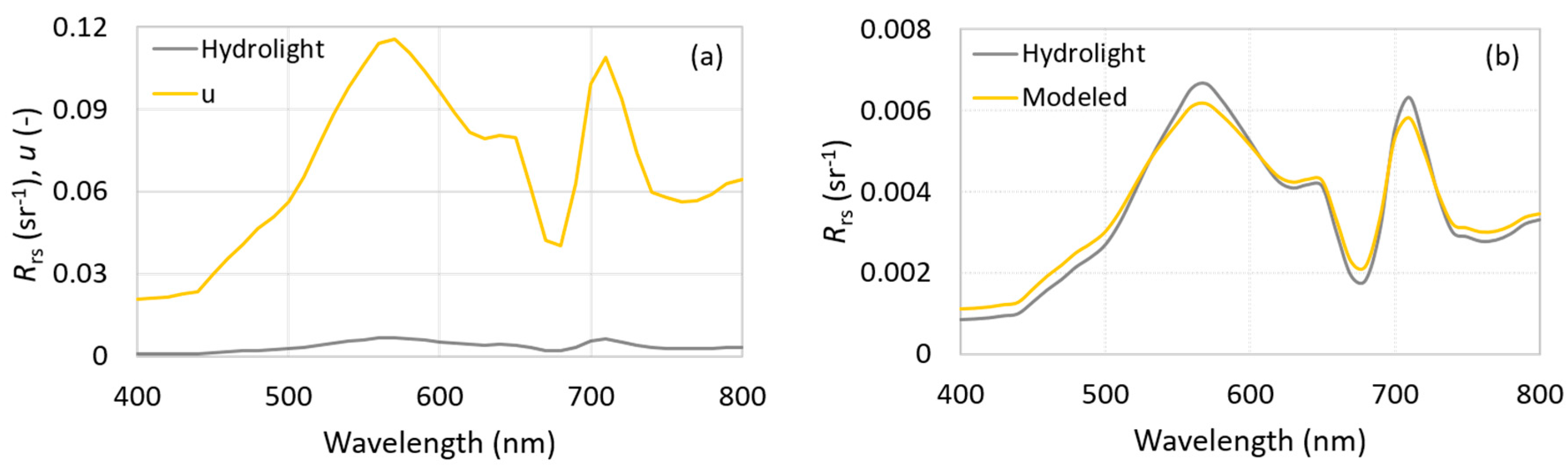
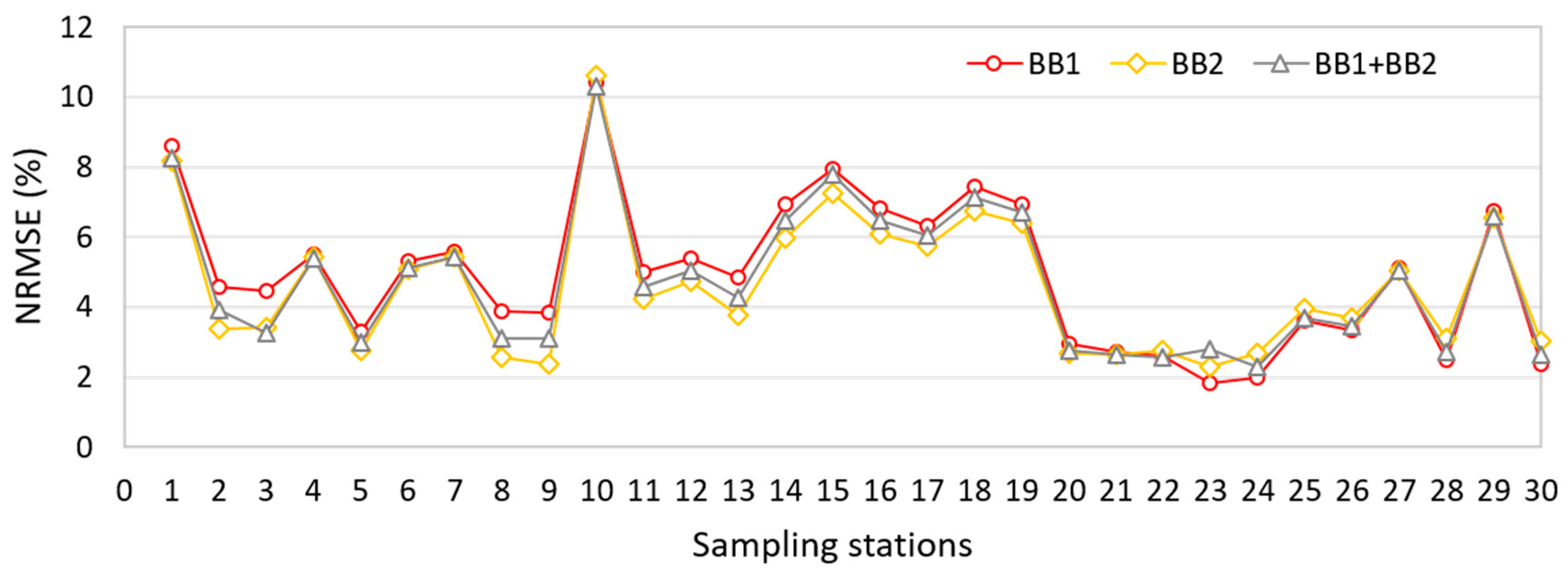
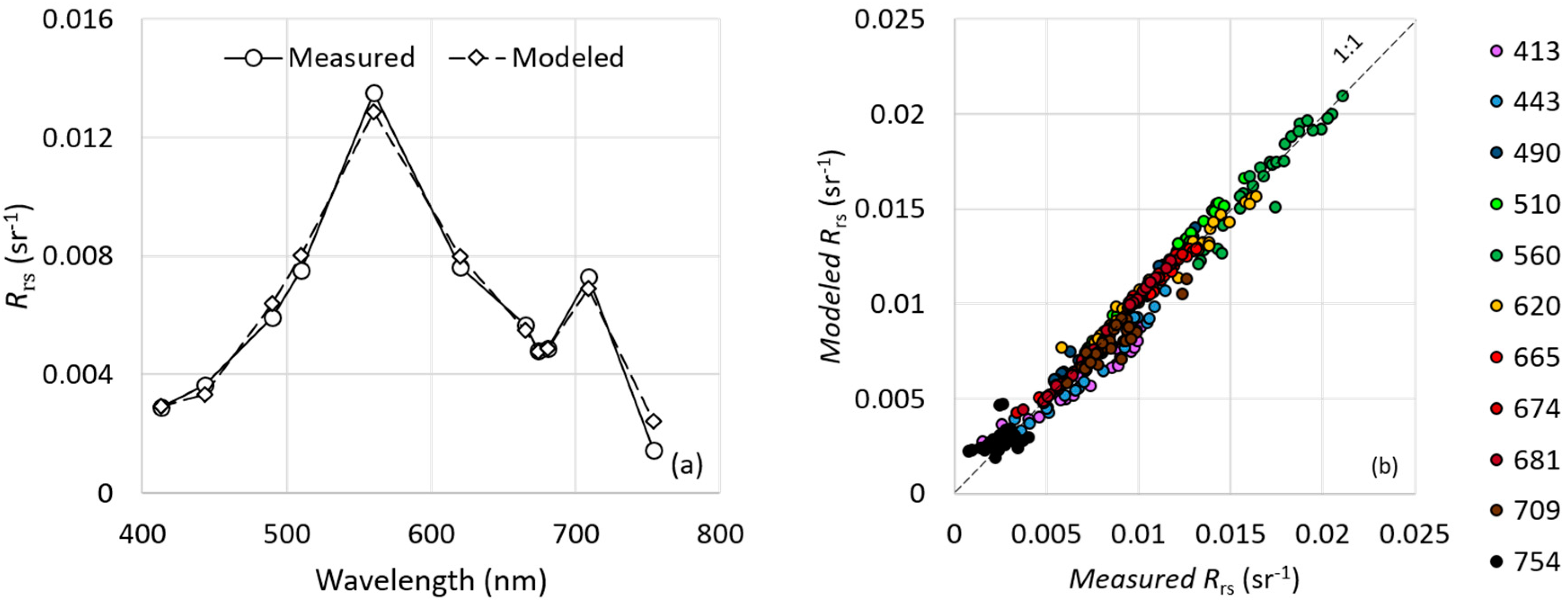
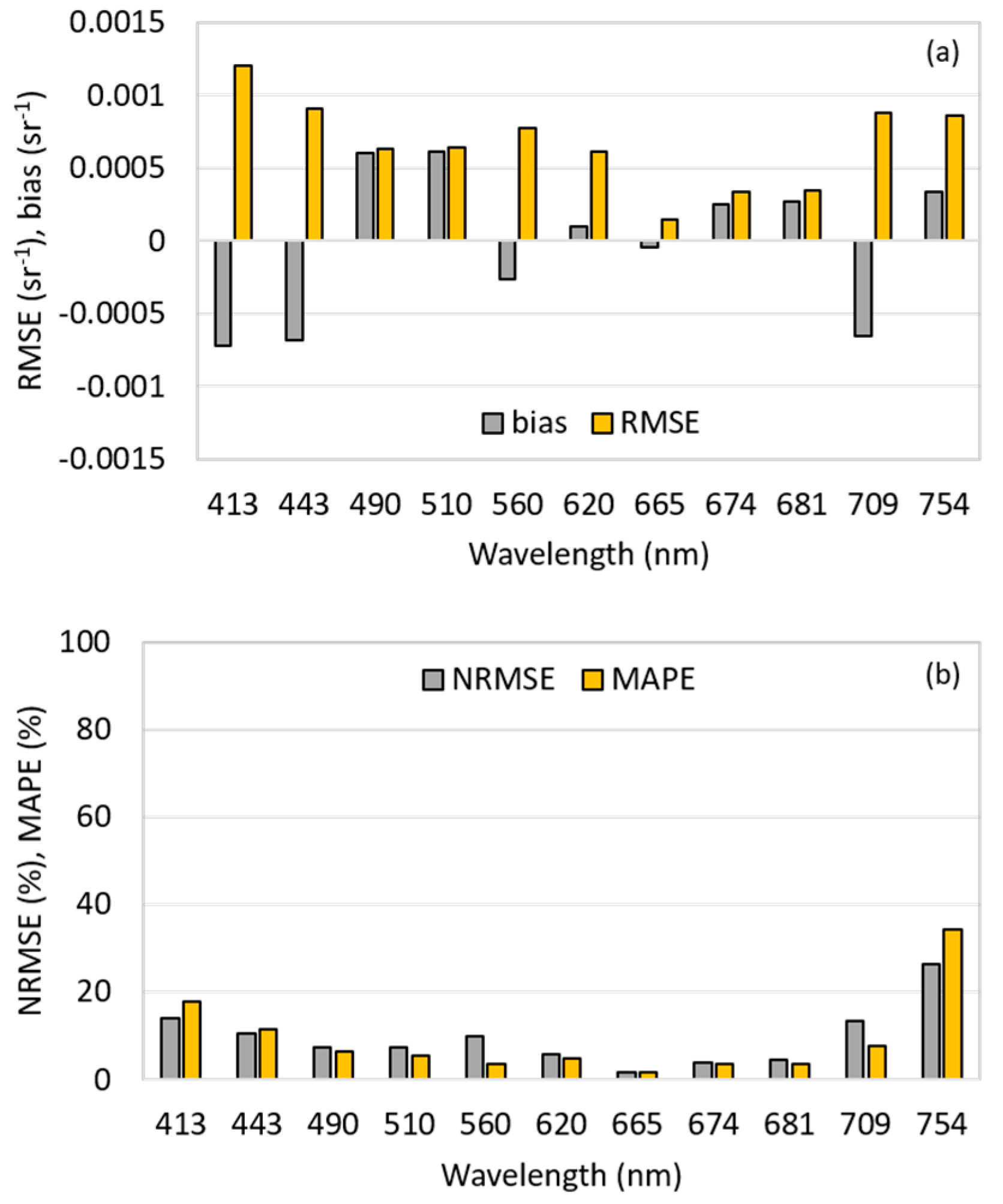
3.4. Inversion of Semi-Analytical Algorithm

The γ value (0.053) was used to calibrate the three semi-analytical models parameterized considering: (a) May dataset; (b) October dataset; and (c) both months’ datasets. The three different semi-analytical algorithms were applied to estimate chl a content in BA in order to validate the performance of the algorithms. Figure 7 shows the NRMSE obtained from the optical closure for each sampling station in BA considering every spectral band used in the fitting. NRMSE was calculated taking into account the 11 bands from the OLCI Sentinel-3 sensor used in parameterizing the semi-analytical algorithm. In general, the inversion of the semi-analytical algorithm yielded accurate adjustments, with errors lower than 11%. The highest NRMSE values were computed for stations 1 and 10 (see Figure 1 for location), with values higher than 8%, which exhibited a chl a content of around 200 mg m⁻³. The best performances were obtained for stations 20 to 24, with chl a ranging from 25–35 mg m⁻³, i.e., the lowest values of chl a concentration. We believe the spectral features become more complex with chl a content increasing, so fitting the model becomes more difficult.

In general, the three semi-analytical algorithms presented statistically similar performances, with an average NRMSE of 4.96%, 4.62% and 4.75% for the BB1, BB2 and BB1 + BB2 datasets, respectively. In this context, the semi-analytical algorithm parameterized using both datasets could be used, representing a higher optical variability. Figure 8a shows the optical closure between the spectrum of R_rs measured for point 3 at the BA reservoir and its spectrum of R_rs derived by using the semi-analytical algorithm parameterized with an average dataset (both the BB1 and BB2 datasets). Among all the sampling points from BA, the third showed the best adjustment for chl a content, with an observed value of 143.9 mg m⁻³ and a model-derived value of 138.0 mg m⁻³. Even so, the overall fitting was satisfactory for practically all sampling stations, as shown in Figure 8b. The sampling points were well distributed around 1:1 line, indicating good adjustment between measured and modeled R_rs for every wavelength.

Figure 9 shows the uncertainties obtained in adjustment for every spectral band, considering bias, RMSE, NRMSE and MAPE. Overall, the highest errors were recorded for the shorter (413 and 443 nm) and longer (709 and 754 nm) wavelengths. Despite that, just 754 nm exhibited NRMSE higher than 25%, while the others displayed NRMSE values lower than 14%. On the other hand, the lowest errors were registered at 665 nm, with NRMSE and MAPE lower than 2% (1.7% and 1.5%, respectively). The other bands in the red spectral region also showed low errors, with NRMSE and MAPE lower than 5%.

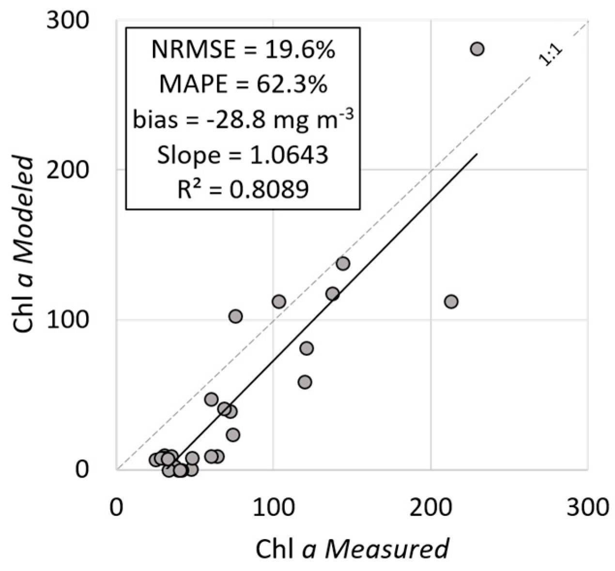
3.5. Estimation of Chl a Concentration

Model parameterized from BB2 dataset showed the best performance in retrieving chl a concentration, with an NRMSE of 18.7%. The main cause of this result was the greater bio-optical similarity between BB2 and BA as opposed to between BB1 and BA. This similarity is mainly associated with the highest chl a concentration observed in BB2 and BA, with maximum chl a of about 700 mg m⁻³. In three cases, the RMSE (43.5, 38.2 and 40.1 mg m⁻³, respectively) were lower than the standard deviation (54.5 mg m⁻³). Although the BB2 dataset produced the best performance, it is statistically equal to the other two developed models. The algorithm designed from both the BB1 and BB2 datasets was therefore tested to estimate chl a content in BA, once they range a higher bio-optical variability (17.7 to 723.5 mg m⁻³).

Figure 10 shows comparisons between measured and modeled chl a, using the semi-analytical algorithm parameterized with absorption measurements acquired in both the BB1 and BB2 datasets. Results of the validation showed a good performance of the semi-analytical algorithm parameterized from both the BB1 and BB2 datasets. A mean NRMSE of 19.6% and a mean MAPE of 62.3% were obtained, close to the values calculated for the BB2 dataset.

4. Discussion

Chl a content exhibited a high variability in both BB and BA, leading to a considerable variation in a^*_φ. In addition, a^*_φ measurements showed high interference by package effect in both BB and BA, with low a^*_φ values (a^*_φ(440) < 0.20 m² mg⁻¹), when compared to other oligotrophic water bodies such as the Nova Avanhandava reservoir, also located on the Tietê River, which gave maximum values of a^*_φ(440) close to 0.40 m² mg⁻¹ [46]. The flattening a^*_φ curve from station 3 (BB2) can be associated with pigment packaging. Station 3 showed the highest chl a concentration for every field campaign (797.8 mg m⁻³). Stations 14 and 18 also showed high concentrations of chl a (723.5 and 713.7 mg m⁻³, respectively) but they did not present flattening of a^*_φ spectra. Nevertheless, these stations were influenced of the absorption by accessory pigments, especially carotenoids [47]. However, these stations were not used for the parameterization because there was no a_NAP spectrum.

The inversion of the semi-analytical algorithm exhibited the best performance in bands of red light (665, 674 and 681 nm), especially at 665 nm. This finding indicates that this wavelength is suitable for retrieving chl a concentration. The wavelength at 620 nm also retrieved accurately, and its use can be considered suitable for predicting phycocyanin content. Only the 754 nm wavelength gave a fit with an NRMSE higher than 20%, which discourages the use of this band for estimating OSCs. Overall, the bands of the OLCI Sentinel-3 sensor exhibited good potential for estimating chl a content accurately in eutrophic waters. For future works, we intend to apply the semi-analytical algorithm in an OLCI Sentinel-3 image, testing other techniques of numerical optimization, such as neural networks.

We also realized that the best adjustment of R_rs is not directly associated with the best estimation of chl a. The semi-analytical algorithm was not capable of retrieving chl a concentrations accurately for stations 8 and 9. These sampling stations exhibited the highest chl a content (higher than 600 mg m⁻³). In these cases, the shape of the R_rs spectra is modeled correctly, but their magnitude is not. This problem is directly related to the pigment packaging issue, in which the a^*_φ magnitude does not produce the pattern expected due to the shadowing effect [48]. This outcome accords with the statement in the previous paragraph, that the higher chl a concentration harms the performance of semi-analytical algorithms.

However, the semi-analytical algorithm parameterized yielded satisfactory results in predicting chl a content in eutrophic reservoirs, with an average NRMSE lower than 20%. We associate this good performance with a dominance of phytoplankton contribution to the a spectra in these environments (results are not presented here). Despite that, a_NAP and a_CDOM measurements cannot be ignored and affect the semi-analytical algorithm performance. It is therefore important, in inland waters, to model the contribution of each OSC correctly before inserting them in the final semi-analytical algorithm.

The semi-analytical algorithm produced good results compared to other bio-optical models parameterized from the BB1 and BB2 datasets [22]. The performance of the numerical optimization was better at estimating the chl a content than the empirical approach. The Oa8/Oa11 ratio (OLCI/Sentinel-3 bands centered at 665 and 709 nm, respectively) produced an NRMSE of 37.8%, while the semi-analytical modeling yielded an NRMSE of 19.6%. In turn, the quasi-analytical algorithm (QAA) yielded the best estimation with an NRMSE = 13.8%. Despite that, the QAA was validated based on a BB dataset, which could have improved its performance. The outcomes obtained in this research can be considered sufficiently accurate.

5. Conclusions

The semi-analytical algorithm designed in this research from data collected in a eutrophic reservoir showed good performance in estimating accurately chl a concentration in a reservoir with high trophic status. The parameterization using both the BB1 and BB2 datasets was capable of predicting a large chl a concentration range in BA. This result was possible due to the high bio-optical variability of the parameters collected in the BB reservoir and similar bio-optical conditions between the BB and BA reservoirs.

Once again, the bio-optical characteristics of water bodies were essential to good performance of the semi-analytical algorithm. The similarity between datasets of BB and BA provides suitable bio-optical conditions for parameterizing an algorithm from BB and applying it to BA. The average values of SIOPs gathered from BB2 produce the better estimations of chl a content. While the average a^*_φ spectra measured in the three field surveys are very similar, the mean spectra from BB2 and BA differ to the greatest extent, as shown in Figure 4. In addition, the variability of the FSS concentration is also more similar in the measurements from BB2 and BA than from BB1 and BA, improving the performance of the semi-analytical algorithm when the average a^*_NAP for BB2 is used.

These findings lead to the conclusion that when similarity occurs between the SIOPs in a semi-analytical model parameterized for a locale, the results can be applied to another locale. The OLCI Sentinel-3 bands exhibited a performance suitable for chl a concentration, since it has the bands associated with the absorption of the spectral features of phytoplankton pigments. In the present form, the semi-analytical algorithm can be applied to OLCI Sentinel-3 images and other products of hyperspectral sensors to estimate chl a concentration. However, other multispectral products also have potential for retrieving OSC from this sort of modeling approach where there are suitable spectral bands. A potential product comes from the MSI Sentinel-2 sensor, with eight bands between 400 and 900 nm.

References

1. Brando, V.E.; Dekker, A.G. Satellite hyperspectral remote sensing for estimating estuarine and coastal water quality. IEEE Trans. Geosci. Remote Sens. 2003, 41, 1378–1387. [Google Scholar] [CrossRef]
2. Watanabe, F.S.Y.; Alcântara, E.; Rodrigues, T.W.P.; Imai, N.N.; Barbosa, C.C.F.; Rotta, L.H.S. Estimation of chlorophyll-a concentration and the trophic state of the Barra Bonita hydroelectric reservoir using OLI/Landsat-8 images. Int. J. Environ. Res. Public Health 2015, 12, 10391–10417. [Google Scholar] [CrossRef] [PubMed]
3. Salem, S.I.; Strand, M.H.; Higa, H.; Kim, H.; Kazuhiro, K.; Oki, K.; Oki, T. Evaluation of MERIS chlorophyll-a retrieval processors in a complex turbid lake Kasumigaura over a 10-year mission. Remote Sens. 2017, 9, 1022. [Google Scholar] [CrossRef]
4. Kirk, J.T.O. Light and Photosynthesis in Aquatic Ecosystems, 3rd ed.; Cambridge University Press: Cambridge, UK, 2011; pp. 199–261. ISBN 978-0-521-15175-7. [Google Scholar]
5. Campbell, G.; Phinn, S.R.; Dekker, A.G.; Brando, V.E. Remote sensing of water quality in an Australian tropical freshwater impoundment using matrix inversion and MERIS images. Remote Sens. Environ. 2011, 115, 2402–2414. [Google Scholar] [CrossRef] [Green Version]
6. Richardson, L.L. Remote sensing of algal bloom dynamics: New research fuses remote sensing of aquatic ecosystems with algal accessory pigment analysis. Bioscience 1996, 46, 492–501. [Google Scholar] [CrossRef]
7. Gordon, H.R.; Brown, O.B.; Evans, R.H.; Brown, J.W.; Smith, R.C.; Baker, K.S.; Clark, D.K. A seminalytical radiance model of ocean color. J. Geophys. Res. 1988, 93, 10909–10924. [Google Scholar] [CrossRef]
8. Mobley, C.D. Light and Water: Radiative Transfer in Natural Waters; Academic Press: San Diego, CA, USA, 1994. [Google Scholar]
9. Hoge, F.E.; Lyon, P.E. Satellite retrieval of inherent optical properties by linear matrix inversion of oceanic radiance models: An analysis of model and radiance measurement errors. J. Geophys. Res. 1996, 101, 16631–16648. [Google Scholar] [CrossRef]
10. Maritorena, S.; Siegel, D.A.; Peterson, A.R. Optimization of a semianalytical ocean color model for global-scale applications. Appl. Opt. 2002, 41, 2705–2714. [Google Scholar] [CrossRef] [PubMed]
11. Yang, W.; Matsushita, B.; Chen, J.; Fukushima, T. Estimating constituent concentrations in case II waters from MERIS satellite data by semi-analytical model optimizing and look-up tables. Remote Sens. Environ. 2011, 115, 1247–1259. [Google Scholar] [CrossRef] [Green Version]
12. Li, L.; Li, L.; Shi, K.; Li, Z.; Song, K. A semi-analytical algorithm for remote estimation of phycocyanin in inland waters. Sci. Total Environ. 2012, 435–436, 141–150. [Google Scholar] [CrossRef] [PubMed]
13. Brando, V.E.; Dekker, A.G.; Park, Y.J.; Schroeder, T. Adaptive semianalytical inversion of ocean color radiometry in optically complex waters. Appl. Opt. 2012, 51, 2808–2833. [Google Scholar] [CrossRef] [PubMed]
14. Pyo, J.C.; Pachepsky, Y.; Baek, S.S.; Kwon, Y.S.; Kim, M.J.; Lee, H.; Park, S.; Cha, Y.K.; Ha, R.; Nam, G.; et al. Optimizing semi-analytical algorithms for estimating chlorophyll-a and phycocyanin concentrations in inland waters in Korea. Remote Sens. 2017, 9, 542. [Google Scholar] [CrossRef]
15. Brando, V.E.; Anstee, J.M.; Wetttle, M.; Dekker, A.G.; Phinn, S.R.; Roelfsema, C. A physcis based retrieval and quality assessment of bathymetry from suboptimal hyperspectral data. Remote Sens. Environ. 2009, 113, 755–770. [Google Scholar] [CrossRef]
16. Rodrigues, T.; Alcântara, E.; Watanabe, F.; Imai, N. Retrieval of Secchi disk depth from reservoir using a semi-analytical scheme. Remote Sens. Environ. 2017, 198, 213–228. [Google Scholar] [CrossRef]
17. Lee, Z.P.; Carder, K.L.; Mobley, C.D.; Steward, R.G.; Patch, J.S. Hyperspectral remote sensing for shallow waters: 2. Deriving bottom depths and water properties by optimization. Appl. Opt. 1999, 38, 3831–3843. [Google Scholar] [CrossRef] [PubMed]
18. Lee, Z.P.; Carder, K.L.; Arnone, R.A. Deriving inherent optical properties from water color: A multiband quasi-analytical algorithm for optically deep waters. Appl. Opt. 2002, 41, 5755–5772. [Google Scholar] [CrossRef] [PubMed]
19. Lee, Z.P.; Carder, K.L.; Chen, R.F.; Peacock, T.G. Properties of the water column and bottom derived from airborne visible infrared imaging spectrometer (AVIRIS) data. J. Geophys. Res. 2001, 106, 11639–11651. [Google Scholar] [CrossRef]
20. Hoogenboom, H.J.; Dekker, A.G.; De Hann, J.F. Retrieval of chlorophyll and suspended matter in inland waters from CASI data by matrix inversion. Can. J. Remote Sens. 1998, 24, 144–152. [Google Scholar] [CrossRef]
21. Barbosa, F.A.R.; Padisák, J.; Espíndola, E.L.G.; Borics, G.; Rocha, O. The cascading reservoir continuum concept (CRCC) and its application to the river Tietê-basin, São Paulo State, Brazil. In Theoretical Reservoir Ecology and Its Application; Tundisi, J.G., Straškraba, M., Eds.; International Institute of Ecology: São Carlos, Brazil, 1999; pp. 425–437. [Google Scholar]
22. Watanabe, F.; Mishra, D.R.; Astuti, I.; Rodrigues, T.; Alcântara, E.; Imai, N.N.; Barbosa, C. Parameterization and calibration of a quasi-analytical algorithm for tropical eutrophic waters. ISPRS J. Photogram. Remote Sens. 2016, 121, 28–47. [Google Scholar] [CrossRef]
23. Dellamano-Oliveira, M.J.; Vieira, A.A.H.; Rocha, O.; Colombo, V.; Sant’Anna, C.L. Phytoplankton taxonomic composition and temporal changes in a tropical reservoir. Arch. Hydrobiol. 2008, 171, 27–38. [Google Scholar] [CrossRef]
24. Tundisi, J.G.; Matsumura-Tundisi, T.; Abe, D.S. The ecological dynamics of Barra Bonita (Tietê River, SP, Brazil) reservoir: Implications for its biodiversity. Braz. J. Biol. 2008, 68, 1079–1098. [Google Scholar] [CrossRef] [PubMed]
25. Tundisi, J.G.; Matsumura-Tundisi, T.; Pereira, K.C.; Luzia, A.P.; Passerini, M.D.; Chiba, W.A.C.; Morais, M.A.; Sebastien, N.Y. Cold fronts and reservoir limnology: An integrated approach towards the ecological dynamics of freshwater ecosystems. Braz. J. Biol. 2010, 70, 815–824. [Google Scholar] [CrossRef] [PubMed]
26. Abe, D.S.; Matsumura-Tundisi, T.; Rocha, O.; Tundisi, J.G. Denitrification and bacterial community structure in the cascade of six reservoirs on a tropical in Brazil. Hydrobiologia 2003, 504, 67–76. [Google Scholar] [CrossRef]
27. Rodrigues, T.W.P.; Guimarães, U.S.; Rotta, L.H.S.; Watanabe, F.S.Y.; Alcântara, E.; Imai, N.N. Delineamento amostral em reservatórios utilizando imagens Landsat-8/OLI: Um estudo de caso no reservatório de Nova Avanhandava (Estado de São Paulo, Brasil). Bol. Ciênc. Geod. 2016, 22, 303–323. [Google Scholar] [CrossRef]
28. Mobley, C.D. Estimation of the remote-sensing reflectance from above-surface measurements. Appl. Opt. 1999, 38, 7442–7455. [Google Scholar] [CrossRef] [PubMed]
29. Lee, Z.P.; Ahn, Y.H.; Mobley, C.; Arnone, R. Removal of surface-reflected light for the measurement of remote-sensing reflectance from an above-surface platform. Opt. Express 2010, 18, 26313–26324. [Google Scholar] [CrossRef] [PubMed]
30. Golterman, H.L.; Clymo, R.S.; Ohnstad, M.A.M. Methods for Physical and Chemical Analysis of Fresh Water; Blackwell Scientific Publications: Oxford, UK, 1978. [Google Scholar]
31. American Public Health Association (APHA); American Water Works Association (AWWA); Water Environment Federation (WEF). Standard Methods for the Examination of Water and Wastewater, 20th ed.; APHA, AWWA, WEF: Washington, DC, USA, 1998; pp. 2–54. [Google Scholar]
32. Tassan, S.; Ferrari, G.M. An alternative approach to absorption measurements of aquatic particles retained on filters. Limnol. Oceanogr. 1995, 40, 1358–1368. [Google Scholar] [CrossRef]
33. Tassan, S.; Ferrari, G. Measurement of light absorption by aquatic particles retained on filters: Determination of the optical pathlength amplification by the ‘transmittance-reflectance’ method. J. Plankton Res. 1998, 20, 1699–1709. [Google Scholar] [CrossRef]
34. Tassan, S.; Ferrari, G.M. A sensitivity analysis of the ‘transmittance-reflectance’ method for measuring light absorption by aquatic particles. J. Plankton Res. 2002, 24, 757–774. [Google Scholar] [CrossRef]
35. Bricaud, A.; Morel, A.; Prieur, L. Absorption by dissolved organic matter of the sea (yellow substance) in the UV and visible domains. Limnol. Oceanogr. 1981, 26, 43–53. [Google Scholar] [CrossRef]
36. Ordematt, D.; Gitelson, A.; Brando, V.E.; Schaepman, M. Review of constituent retrieval in optically deep and complex waters from satellite imagery. Remote Sens. Environ. 2012, 118, 116–126. [Google Scholar] [CrossRef] [Green Version]
37. Smith, R.C.; Baker, K.S. Optical properties of the clearest natural waters (200–800 nm). Appl. Opt. 1981, 20, 177–184. [Google Scholar] [CrossRef] [PubMed]
38. Lee, Z.P.; Carder, K.L. Absorption spectrum of phytoplankton pigments derived from hyperspectral remote-sensing reflectance. Remote Sens. Environ. 2004, 89, 361–368. [Google Scholar] [CrossRef]
39. Mishra, S.; Mishra, D.R.; Lee, Z.P. Bio-optical inversion in highly turbid and cyanobacteria-dominated waters. IEEE Trans. Geosci. Remote Sens. 2014, 52, 375–388. [Google Scholar] [CrossRef]
40. Mobley, C.D.; Sundmann, L.K. Hydrolight 5.2 and Ecolight 5.2 User’s Guide; Sequoia Scientific: Bellevue, WA, USA, 2013. [Google Scholar]
41. Dolon, C.; Berruti, B.; Buomgiorno, A.; Ferreira, M.H.; Féménias, P.; Frerick, J.; Goryl, P.; Klein, U.; Laur, H.; Mavrocordatos, C.; et al. The global monitoring for environment and security (GMES) Sentinel-3 mission. Remote Sens. Environ. 2012, 120, 37–57. [Google Scholar] [CrossRef]
42. Weaver, E.C.; Wrigley, R. Factors Affecting the Identification of Phytoplankton Groups by Means of Remote Sensing; NASA, Ames Research Center: Moffet Field, CA, USA, 1994. [Google Scholar]
43. Simis, S.G.H.; Peters, S.W.M.; Gons, H.J. Remote sensing of the cyanobacterial pigment phycocyanin in turbid inland water. Limnol. Oceanogr. 2005, 50, 237–245. [Google Scholar] [CrossRef]
44. Doerffer, R.; Schiller, H. The MERIS Case 2 water algorithm. Int. J. Remote Sens. 2007, 28, 517–535. [Google Scholar] [CrossRef]
45. Santini, F.; Alberotanza, L.; Cavalli, R.M.; Pignatti, S. A two-step optimization procedure for assessing water constituent concentrations by hyperspectral remote sensing techniques: An application to the highly turbid Venice lagoon waters. Remote Sens. Environ. 2010, 114, 887–898. [Google Scholar] [CrossRef]
46. Rodrigues, T.W.P. From Oligo to Eutrophic Inland Waters: Advancements and Challenges for Bio-Optical Modeling. Ph.D. Thesis, Universidade Estadual Paulista, Presidente Prudente, Brazil, March 2016. [Google Scholar]
47. Bidigare, R.R.; Ondrusek, M.E.; Morrow, J.H.; Kiefer, D.A. In vivo absorption properties of algal pigments. Proc. SPIE 1990, 1302, 290–309. [Google Scholar]
48. Alcântara, E.; Watanabe, F.; Rodrigues, T.; Bernardo, N. An investigation into the phytoplankton package effect on the chlorophyll-a specific absorption coefficient in Barra Bonita reservoir, Brazil. Remote Sens. Lett. 2016, 7, 761–770. [Google Scholar] [CrossRef]
Figure 1. (a) Reservoir cascade system from the Tietê River, São Paulo State (Brazil), and the location of sampling stations in (b) Barra Bonita and (c) Bariri reservoirs.
Remotesensing 10 00227 g001
Figure 2. Scatterplot between chl a and TSS concentration for BB1, BB2 and BA.
Remotesensing 10 00227 g002
Figure 3. Boxplot of concentrations of (a) chl a and (b) fixed suspended solids (FSS) acquired in BB1, BB2 and BA.
Remotesensing 10 00227 g003
Figure 4. Rrs spectra measured in situ for following field surveys: (a) BB1; (b) BB2; and (c) BA.
Remotesensing 10 00227 g004
Figure 5. Average specific-chlorophyll absorption coefficient, a*φ, measured, with minimum and maximum, collected in (a) BB1; (b) BB2 and (c) BA; and (d) comparison of the average a*φ for the three field surveys.
Remotesensing 10 00227 g005
Figure 6. Comparison between (a) average Rrs and u spectra, both simulated via Hydrolight and between (b) average Rrs spectra simulated by Hydrolight and modeled from u and γ.
Remotesensing 10 00227 g006
Figure 7. Normalized root mean square error (NRMSE) between simulated and modeled Rrs calculated considering the 11 bands for each sampling station from BA reservoir, obtained from the semi-analytical algorithm parameterized for both BB1 and BB2 datasets.
Remotesensing 10 00227 g007
Figure 8. Optical closure between (a) the in situ measured Rrs and modeled Rrs from the semi-analytical algorithm applied to retrieve chl a concentration in point 3/BA. Scatterplot of (b) measured and modeled Rrs, considering every band (nm) individually.
Remotesensing 10 00227 g008
Figure 9. Error analysis for every Ocean and Land Colour Instrument (OLCI) band used in the model adjustment. Plot of (a) bias and root mean square error (RMSE), and (b) NRMSE and mean absolute percentage error (MAPE).
Remotesensing 10 00227 g009
Figure 10. Validation of the semi-analytical algorithm parameterized using average a*φ measured in BB applied to the dataset collected in BA in August 2016.
Remotesensing 10 00227 g010