Exploiting Satellite-Based Surface Soil Moisture for Flood Forecasting in the Mediterranean Area: State Update Versus Rainfall Correction


Abstract
:
1. Introduction
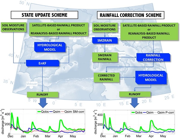
- To what extent updating soil moisture states leads to better flood predictions than the correction of the rainfall?
- How much these improvements are affected by the underlying accuracy of the original rainfall product used for forcing the hydrological model?
- What is the impact of the basin size and the climate conditions on the results?
2. Material
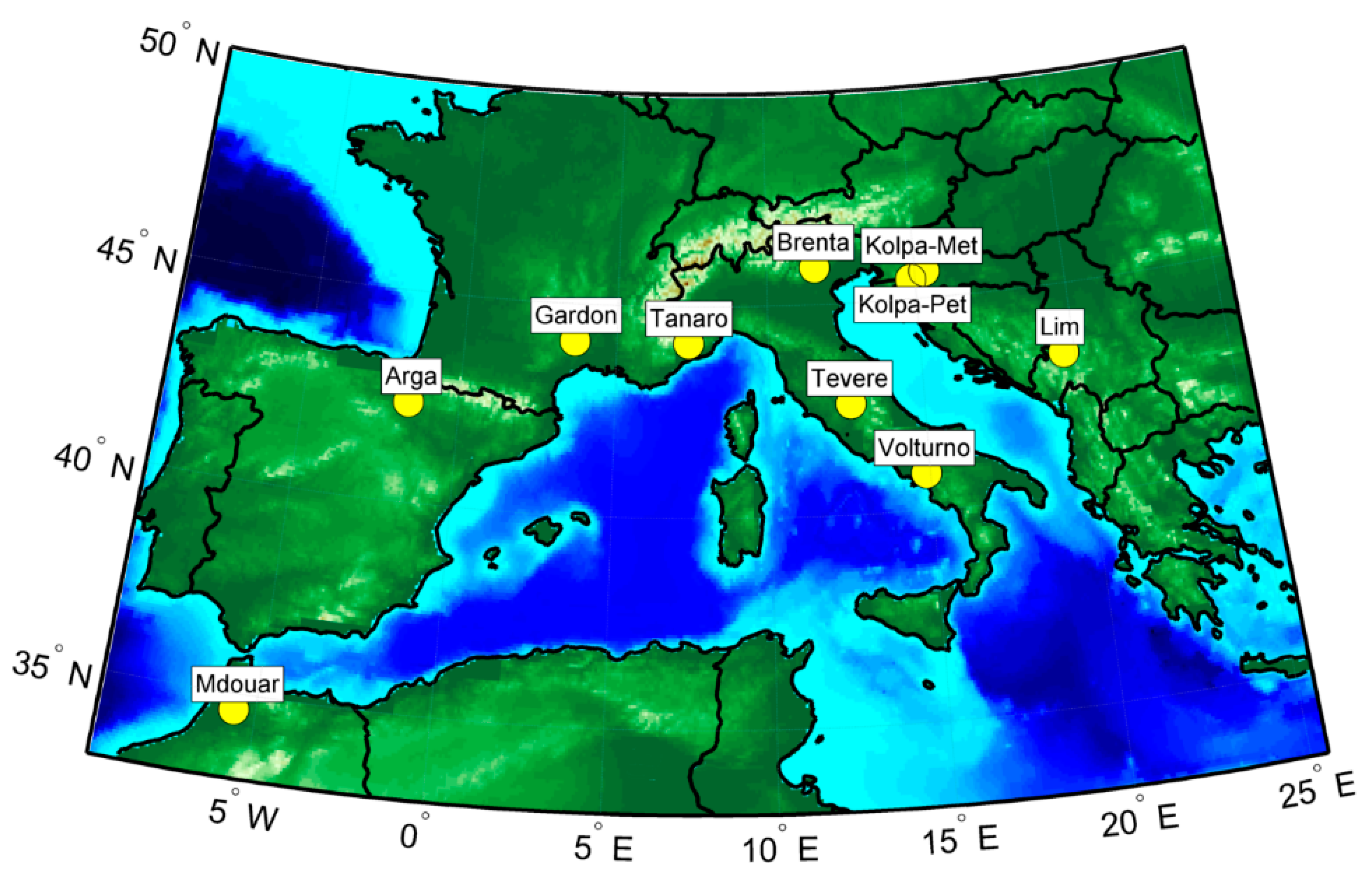
2.1. Study Area
2.2. Datasets
2.2.1. Soil Moisture Observations
2.2.2. Rainfall and Temperature Data
2.2.3. Stream Flow Data
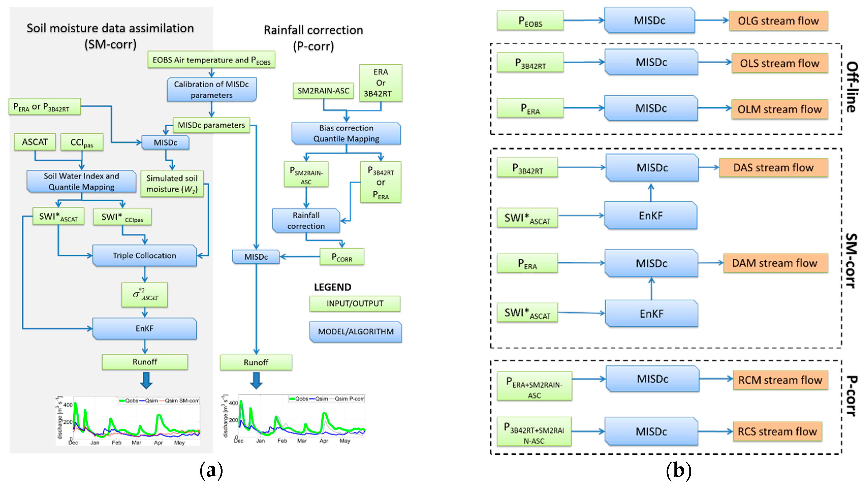
3. Methods
3.1. MISDc
3.2. Soil Moisture Data Assimilation
3.2.1. Pre-Processing of Soil Moisture Observations and Error Estimation
3.2.2. The Ensemble Kalman Filter
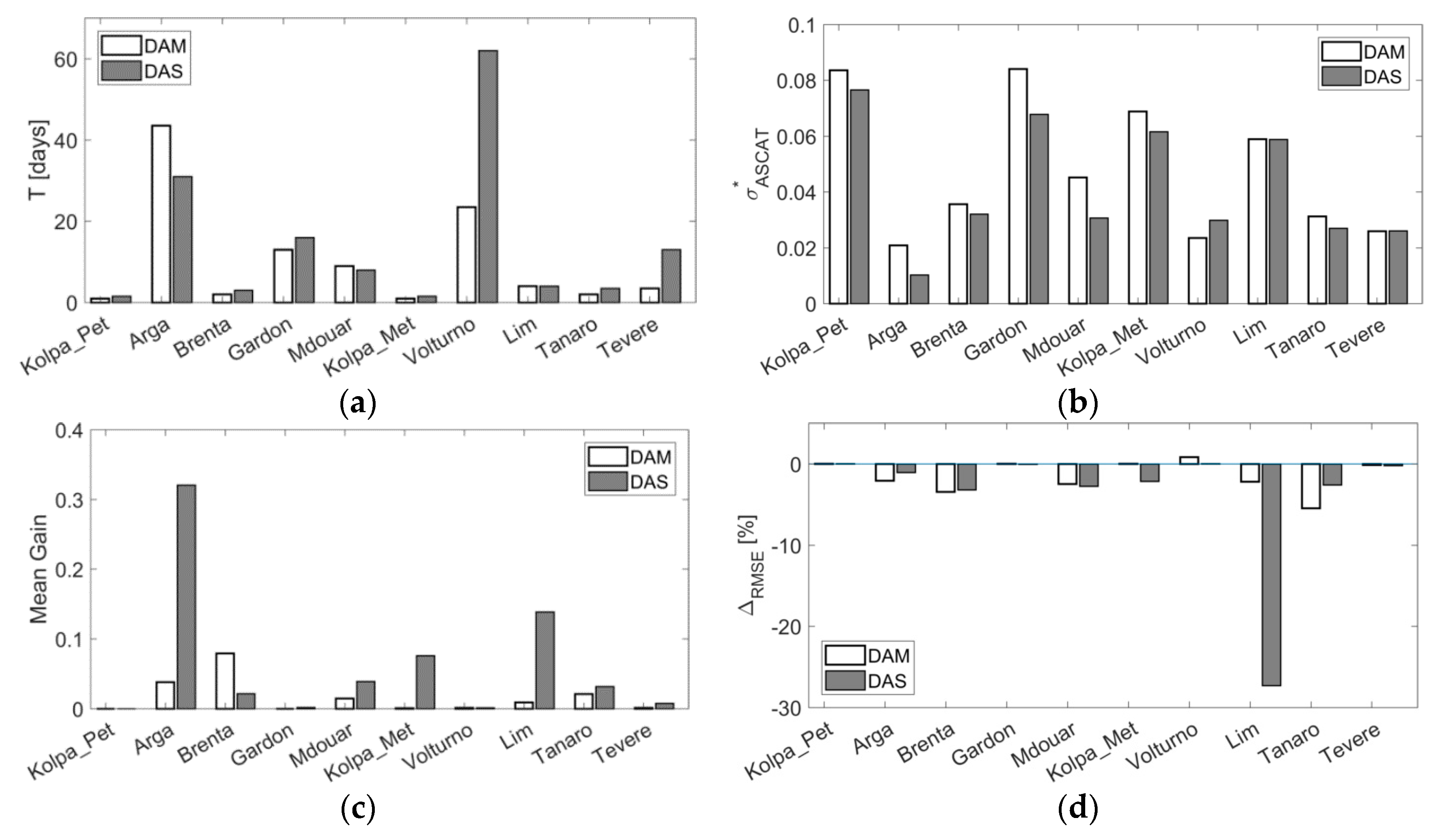
3.2.3. Filter Calibration
3.3. Rainfall Correction
3.3.1. Pre-Processing of Rainfall Observations
3.3.2. Rainfall Integration
3.4. Performance Metrics
3.5. Method Implementation
4. Results and Discussion
4.1. MISDc Model Calibration and Validation Forced with Ground-Based Data
4.2. Satellite Soil Moisture Pre-Processing and Filter Calibration
4.3. Rainfall Correction Calibration
4.4. Rainfall Evaluation
4.5. Stream Flow Evaluation
5. Conclusions
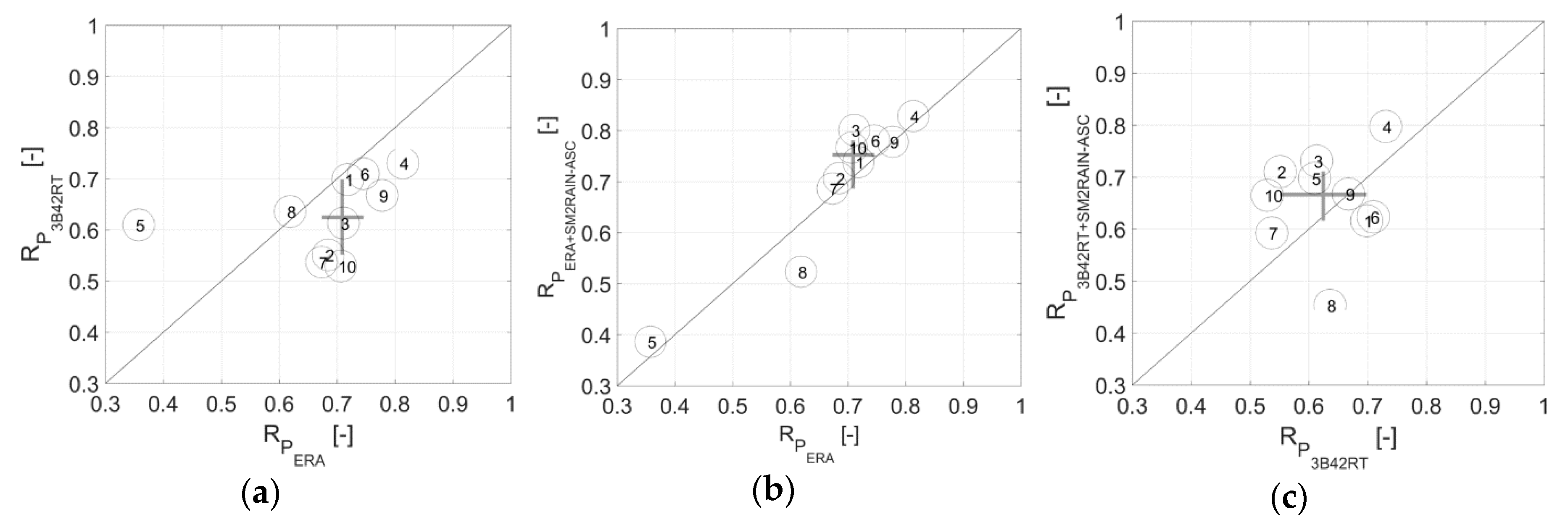
- The gauge-based rainfall dataset (EOBS) performs satisfactorily well over the Mediterranean area with median ANSE and KGE values close to 0.5 (in validation) for the investigated catchments while PERA and P3B42RT provide poorer stream flow predictions.
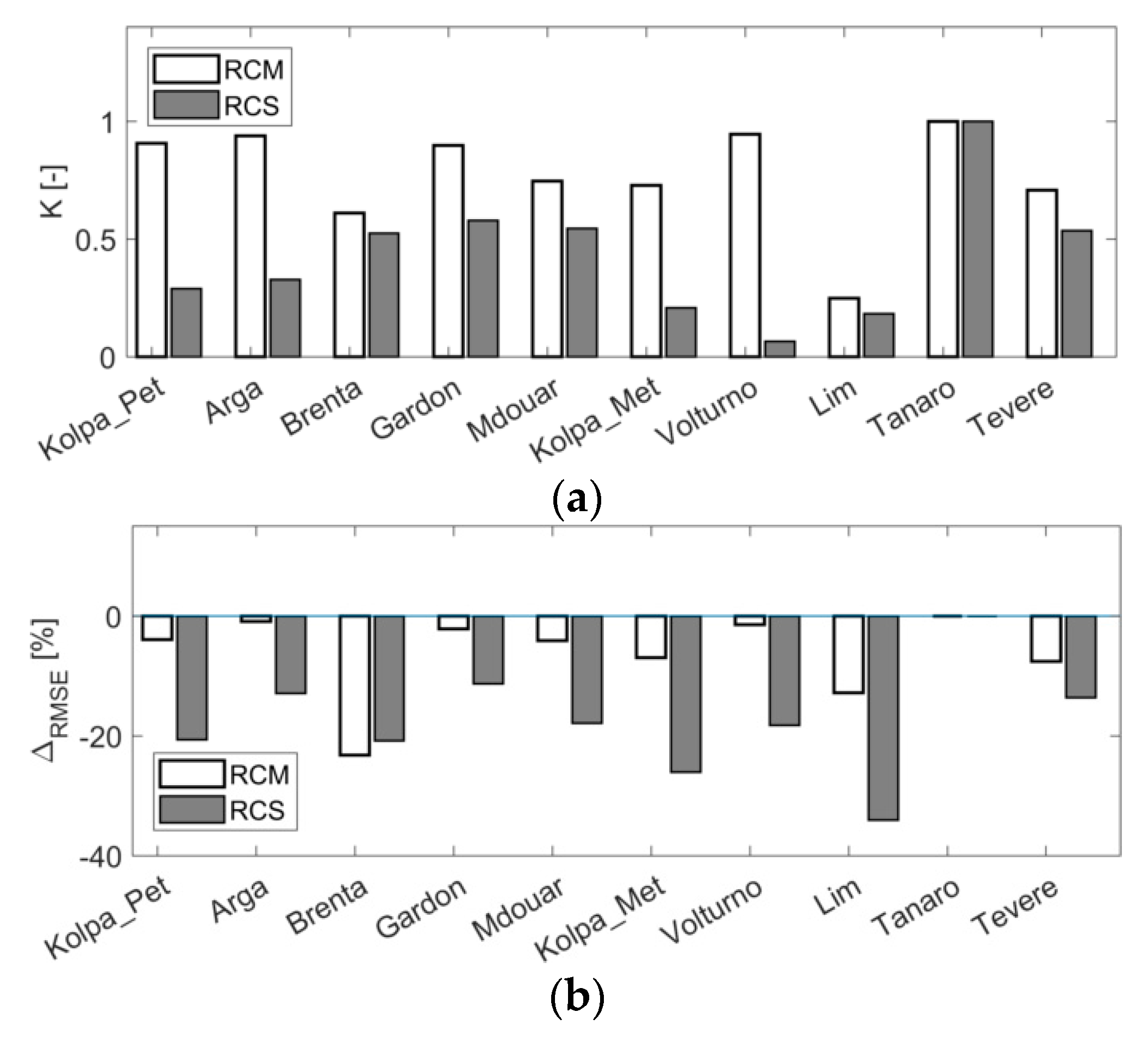
- The soil moisture correction produces an overall slight improvement in terms of median KGE and ANSE scores (4.25% and 1.5% for ERA-Interim and 9.6% and 7.6% for 3B42RT, respectively) whereas the rainfall correction provides a much larger impact with an increase in KGE and ANSE values equal to 14.81 and 7.3% for ERA and 71.8 and 100% for 3B42RT, respectively. In summary, the impact of the rainfall correction for flood simulation is much larger than the soil moisture correction and is consistently higher when the quality of the non-corrected rainfall forcing is poor. Conversely, for low flows, the soil moisture correction schemes provide slight better results but these improvements are limited.
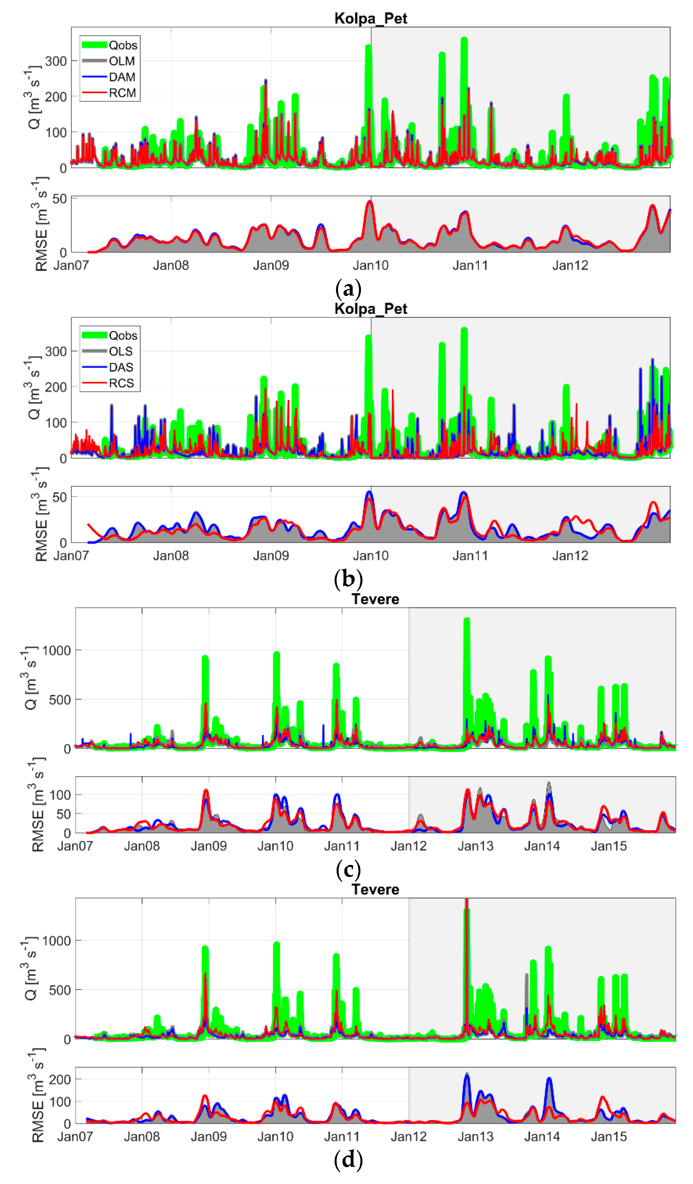
- After the rainfall correction, the simulation run using the satellite-based product (i.e., 3B42RT) shows KGE scores larger than those obtained by using ground-based observations (EOBS). This is an encouraging result that demonstrates the potentiality to improve operational stream flow forecasting by using remotely sensed surface soil moisture.
- The climate, the specific catchment hydrology/model configuration/data assimilation set up and the pre-processing steps associated with the two schemes exert a remarkable effect on the results that complicates the answer to weather is preferable correcting rainfall or updating the model states.
Acknowledgments
Author Contributions
Conflicts of Interest
References
- Beck, H.E.; de Jeu, R.A.; Schellekens, J.; van Dijk, A.I.; Bruijnzeel, L.A. Improving curve number based storm runoff estimates using soil moisture proxies. IEEE J. Sel. Top. Appl. Earth Obs. Remote Sens. 2009, 2, 250–259. [Google Scholar] [CrossRef]
- Koster, R.D.; Mahanama, S.P.; Livneh, B.; Lettenmaier, D.P.; Reichle, R.H. Skill in stream flow forecasts derived from large-scale estimates of soil moisture and snow. Nat. Geosci. 2010, 3, 613–616. [Google Scholar] [CrossRef]
- Matgen, P.; Fenicia, F.; Heitz, S.; Plaza, D.; de Keyser, R.; Pauwels, V.R.; Wagner, W.; Savenije, H. Can ASCAT-derived soil wetness indices reduce predictive uncertainty in well-gauged areas? A comparison with in situ observed soil moisture in an assimilation application. Adv. Water Resour. 2012, 44, 49–65. [Google Scholar] [CrossRef]
- Massari, C.; Brocca, L.; Moramarco, T.; Tramblay, Y.; Lescot, J.F.D. Potential of soil moisture observations in flood modelling: Estimating initial conditions and correcting rainfall. Adv. Water Resour. 2014, 74, 44–53. [Google Scholar] [CrossRef]
- Crow, W.T.; Zhan, X. Continental-scale evaluation of remotely sensed soil moisture products. IEEE Geosci. Remote Sens. Lett. 2007, 4, 451–455. [Google Scholar] [CrossRef]
- Renzullo, L.J.; Van Dijk, A.I.; Perraud, J.M.; Collins, D.; Henderson, B.; Jin, H.; Smith, A.B.; McJannet, D.L. Continental satellite soil moisture data assimilation improves root-zone moisture analysis for water resources assessment. J. Hydrol. 2014, 519, 2747–2762. [Google Scholar] [CrossRef]
- López López, P.; Wanders, N.; Schellekens, J.; Renzullo, L.J.; Sutanudjaja, E.H.; Bierkens, M.F.P. Improved large-scale hydrological modelling through the assimilation of stream flow and downscaled satellite soil moisture observations. Hydrol. Earth Syst. Sci. 2016, 20, 3059–3076. [Google Scholar] [CrossRef]
- Romano, N. Soil moisture at local scale: Measurements and simulations. J. Hydrol. 2014, 516, 6–20. [Google Scholar] [CrossRef]
- Mohanty, B.P.; Cosh, M.H.; Lakshmi, V.; Montzka, C. Soil moisture remote sensing: State-of-the-science. Vadose Zone J. 2017, 16, 1–9. [Google Scholar] [CrossRef]
- Brocca, L.; Melone, F.; Moramarco, T.; Singh, V.P. Assimilation of observed soil moisture data in storm rainfall-runoff modeling. J. Hydrol. Eng. 2009, 14, 153–165. [Google Scholar] [CrossRef]
- Chen, F.; Crow, W.T.; Starks, P.J.; Moriasi, D.N. Improving hydrologic predictions of a catchment model via assimilation of surface soil moisture. Adv. Water Resour. 2011, 34, 526–536. [Google Scholar] [CrossRef]
- Crow, W.T.; Bindlish, R.; Jackson, T.J. The added value of spaceborne passive microwave soil moisture retrievals for forecasting rainfall-runoff partitioning. Geophys. Res. Lett. 2005, 32. [Google Scholar] [CrossRef]
- Brocca, L.; Moramarco, T.; Melone, F.; Wagner, W.; Hasenauer, S.; Hahn, S. Assimilation of surface-and root-zone ASCAT soil moisture products into rainfall–runoff modeling. IEEE Trans. Geosci. Remote Sens. 2011, 50, 2542–2555. [Google Scholar] [CrossRef]
- Alvarez-Garreton, C.; Ryu, D.; Western, A.W.; Su, C.H.; Crow, W.T.; Robertson, D.E.; Leahy, C. Improving operational flood ensemble prediction by the assimilation of satellite soil moisture: Comparison between lumped and semi-distributed schemes. Hydrol. Earth Syst. Sci. 2015, 19, 1659–1676. [Google Scholar] [CrossRef]
- Lievens, H.; Tomer, S.K.; Al Bitar, A.; De Lannoy, G.J.; Drusch, M.; Dumedah, G.; Franssen, H.J.; Kerr, Y.H.; Martens, B.; Pan, M.; et al. SMOS soil moisture assimilation for improved hydrologic simulation in the Murray Darling Basin, Australia. Remote Sens. Environ. 2015, 168, 146–162. [Google Scholar] [CrossRef] [Green Version]
- Massari, C.; Brocca, L.; Tarpanelli, A.; Moramarco, T. Data assimilation of satellite soil moisture into rainfall-runoff modelling: A complex recipe? Remote Sens. 2015, 7, 11403–11433. [Google Scholar] [CrossRef]
- Cenci, L.; Laiolo, P.; Gabellani, S.; Campo, L.; Silvestro, F.; Delogu, F.; Boni, G.; Rudari, R. Assimilation of H-SAF soil moisture products for flash flood early warning systems. Case study: Mediterranean catchments. IEEE J. Sel. Top. Appl. Earth Obs. Remote Sens. 2016, 9, 5634–5646. [Google Scholar] [CrossRef]
- Laiolo, P.; Gabellani, S.; Campo, L.; Silvestro, F.; Delogu, F.; Rudari, R.; Pulvirenti, L.; Boni, G.; Fascetti, F.; Pierdicca, N.; et al. Impact of different satellite soil moisture products on the predictions of a continuous distributed hydrological model. Int. J. Appl. Earth Obs. Geoinf. 2016, 48, 131–145. [Google Scholar] [CrossRef]
- Brown, M.E.; Escobar, V.; Moran, S.; Entekhabi, D.; O’Neill, P.E.; Njoku, E.G.; Doorn, B.; Entin, J.K. NASA’s soil moisture active passive (SMAP) mission and opportunities for applications users. Bull. Am. Meteorol. Soc. 2013, 94, 1125–1128. [Google Scholar] [CrossRef]
- Lievens, H.; Reichle, R.H.; Liu, Q.; De Lannoy, G.J.M.; Dunbar, R.S.; Kim, S.B.; Das, N.N.; Cosh, M.; Walker, J.P.; Wagner, W. Joint Sentinel-1 and SMAP data assimilation to improve soil moisture estimates. Geophys. Res. Lett. 2017, 44, 6145–6153. [Google Scholar] [CrossRef]
- Cenci, L.; Pulvirenti, L.; Boni, G.; Chini, M.; Matgen, P.; Gabellani, S.; Campo, L.; Silvestro, F.; Versace, C.; Campanella, P.; et al. Satellite soil moisture assimilation: Preliminary assessment of the Sentinel 1 potentialities. In Proceedings of the 2016 IEEE International Geoscience and Remote Sensing Symposium (IGARSS), Beijing, China, 10–15 July 2016; pp. 3098–3101. [Google Scholar]
- Crow, W.T.; van Den Berg, M.J.; Huffman, G.J.; Pellarin, T. Correcting rainfall using satellite-based surface soil moisture retrievals: The Soil Moisture Analysis Rainfall Tool (SMART). Water Resour. Res. 2011, 47. [Google Scholar] [CrossRef]
- Pellarin, T.; Louvet, S.; Gruhier, C.; Quantin, G.; Legout, C. A simple and effective method for correcting soil moisture and precipitation estimates using AMSR-E measurements. Remote Sens. Environ. 2013, 136, 28–36. [Google Scholar] [CrossRef]
- Brocca, L.; Ciabatta, L.; Massari, C.; Moramarco, T.; Hahn, S.; Hasenauer, S.; Kidd, R.; Dorigo, W.; Wagner, W.; Levizzani, V. Soil as a natural rain gauge: Estimating global rainfall from satellite soil moisture data. J. Geophys. Res. Atmos. 2014, 119, 5128–5141. [Google Scholar] [CrossRef]
- Ciabatta, L.; Brocca, L.; Massari, C.; Moramarco, T.; Puca, S.; Rinollo, A.; Gabellani, S.; Wagner, W. Integration of satellite soil moisture and rainfall observations over the Italian territory. J. Hydrometeorol. 2015, 16, 1341–1355. [Google Scholar] [CrossRef]
- Koster, R.D.; Brocca, L.; Crow, W.T.; Burgin, M.S.; De Lannoy, G.J. Precipitation estimation using L-band and C-band soil moisture retrievals. Water Resour. Res. 2016, 52, 7213–7225. [Google Scholar] [CrossRef]
- Román-Cascón, C.; Pellarin, T.; Gibon, F.; Brocca, L.; Cosme, E.; Crow, W.; Fernández-Prieto, D.; Kerr, Y.H.; Massari, C. Correcting satellite-based precipitation products through SMOS soil moisture data assimilation in two land-surface models of different complexity: API and SURFEX. Remote Sens. Environ. 2017, 200, 295–310. [Google Scholar] [CrossRef]
- Crow, W.T.; Ryu, D. A new data assimilation approach for improving runoff prediction using remotely-sensed soil moisture retrievals. Hydrol. Earth Syst. Sci. 2009, 13, 1–16. [Google Scholar] [CrossRef]
- Chen, F.; Crow, W.T.; Ryu, D. Dual forcing and state correction via soil moisture assimilation for improved rainfall–runoff modeling. J. Hydrometeorol. 2014, 15, 1832–1848. [Google Scholar] [CrossRef]
- Alvarez-Garreton, C.; Ryu, D.; Western, A.W.; Crow, W.T.; Su, C.H.; Robertson, D.R. Dual assimilation of satellite soil moisture to improve stream flow prediction in data-scarce catchments. Water Resour. Res. 2016, 52, 5357–5375. [Google Scholar] [CrossRef]
- Evensen, G. Data Assimilation: The Ensemble Kalman Filter; Springer: Berlin, Germany, 2009. [Google Scholar]
- Huffman, G.J.; Bolvin, D.T.; Nelkin, E.J.; Wolff, D.B.; Adler, R.F.; Gu, G.; Hong, Y.; Bowman, K.P.; Stocker, E.F. The TRMM multisatellite precipitation analysis (TMPA): Quasi-global, multiyear, combined-sensor precipitation estimates at fine scales. J. Hydrometeorol. 2007, 8, 38–55. [Google Scholar] [CrossRef]
- Wagner, W.; Hahn, S.; Kidd, R.; Melzer, T.; Bartalis, Z.; Hasenauer, S.; Figa-Saldaña, J.; de Rosnay, P.; Jann, A.; Schneider, S.; et al. The ASCAT soil moisture product: A review of its specifications, validation results, and emerging applications. Meteorol. Z. 2013, 22, 5–33. [Google Scholar] [CrossRef]
- Kerr, Y.H.; Waldteufel, P.; Wigneron, J.P.; Delwart, S.; Cabot, F.; Boutin, J.; Escorihuela, M.J.; Font, J.; Reul, N.; Gruhier, C.; et al. The SMOS mission: New tool for monitoring key elements of the global water cycle. Proc. IEEE 2010, 98, 666–687. [Google Scholar] [CrossRef] [Green Version]
- Brocca, L.; Melone, F.; Moramarco, T. Distributed rainfall-runoff modelling for flood frequency estimation and flood forecasting. Hydrol. Process. 2011, 25, 2801–2813. [Google Scholar] [CrossRef]
- Dee, D.P.; Uppala, S.M.; Simmons, A.J.; Berrisford, P.; Poli, P.; Kobayashi, S.; Andrae, U.; Balmaseda, M.A.; Balsamo, G.; Bauer, P.; et al. The ERA-Interim reanalysis: Configuration and performance of the data assimilation system. Q. J. R. Meteorol. Soc. 2011, 137, 553–597. [Google Scholar] [CrossRef]
- Beck, H.E.; Vergopolan, N.; Pan, M.; Levizzani, V.; van Dijk, A.I.; Weedon, G.P.; Brocca, L.; Pappenberger, F.; Huffman, G.J.; Wood, E.F. Global-scale evaluation of 22 precipitation datasets using gauge observations and hydrological modeling. Hydrol. Earth Syst. Sci. 2017, 21, 6201–6217. [Google Scholar] [CrossRef]
- Brocca, L.; Hasenauer, S.; Lacava, T.; Melone, F.; Moramarco, T.; Wagner, W.; Dorigo, W.; Matgen, P.; Martínez-Fernández, J.; Llorens, P.; et al. Soil moisture estimation through ASCAT and AMSR-E sensors: An intercomparison and validation study across Europe. Remote Sens. Environ. 2011, 115, 3390–3408. [Google Scholar] [CrossRef]
- Paulik, C.; Dorigo, W.; Wagner, W.; Kidd, R. Validation of the ASCAT Soil Water Index using in situ data from the International Soil Moisture Network. Int. J. Appl. Earth Obs. Geoinf. 2014, 30, 1–8. [Google Scholar] [CrossRef]
- Dorigo, W.; Wagner, W.; Albergel, C.; Albrecht, F.; Balsamo, G.; Brocca, L.; Chung, D.; Ertl, M.; Forkel, M.; Gruber, A.; et al. ESA CCI soil moisture for improved Earth system understanding: State-of-the art and future directions. Remote Sens. Environ. 2017, 203, 185–215. [Google Scholar] [CrossRef]
- Haylock, M.R.; Hofstra, N.; Klein Tank, A.M.G.; Klok, E.J.; Jones, P.D.; New, M. A European daily high-resolution gridded data set of surface temperature and precipitation for 1950–2006. J. Geophys. Res. Atmos. 2008, 113, 1–12. [Google Scholar] [CrossRef]
- Stampoulis, D.; Anagnostou, E.N. Evaluation of Global Satellite Rainfall Products over Continental Europe. J. Hydrometeorol. 2012, 13, 588–603. [Google Scholar] [CrossRef]
- SM2RAIN-ASCAT (1 January 2007–31 December 2015) European Rainfall Dataset (0.25 Degree/Daily). Available online: http://dx.doi.org/10.13140/RG.2.1.4068.6481/1 (accessed on 13 February 2018).
- Massari, C.; Crow, W.; Brocca, L. An assessment of the performance of global rainfall estimates without ground-based observations. Hydrol. Earth Syst. Sci. 2017, 21, 4347–4361. [Google Scholar] [CrossRef]
- Masseroni, D.; Cislaghi, A.; Camici, S.; Massari, C.; Brocca, L. A reliable rainfall–runoff model for flood forecasting: Review and application to a semi-urbanized watershed at high flood risk in Italy. Hydrol. Res. 2017, 48, 726–740. [Google Scholar] [CrossRef]
- Doorenbos, J.; Pruitt, W.O. Background and Development of Methods to Predict Reference Crop Evapotranspiration (ETo). In Crop Water Requirements. FAO Irrigation and Drainage Paper No. 24; FAO: Rome, Italy, 1977; Appendix II; pp. 108–119. [Google Scholar]
- Famiglietti, J.S.; Wood, E.F. Multiscale modeling of spatially variable water and energy balance processes. Water Resour. Res. 1994, 30, 3061–3078. [Google Scholar] [CrossRef]
- Andreadis, K.M.; Clark, E.A.; Wood, A.W.; Hamlet, A.F.; Lettenmaier, D.P. Twentieth-century drought in the conterminous United States. J. Hydrometeorol. 2005, 6, 985–1001. [Google Scholar] [CrossRef]
- Melone, F.; Corradini, C.; Singh, V.P. Lag prediction in ungauged basins: An investigation through actual data of the upper Tevere River valley. Hydrol. Processes 2002, 16, 1085–1094. [Google Scholar] [CrossRef]
- Wagner, W.; Lemoine, G.; Rott, H. A method for estimating soil moisture from ERS scatterometer and soil data. Remote Sens. Environ. 1999, 70, 191–207. [Google Scholar] [CrossRef]
- Albergel, C.; Rüdiger, C.; Pellarin, T.; Calvet, J.C.; Fritz, N.; Froissard, F.; Suquia, D.; Petitpa, A.; Piguet, B.; Martin, E. From near-surface to root-zone soil moisture using an exponential filter: An assessment of the method based on in-situ observations and model simulations. Hydrol. Earth Syst. Sci. 2008, 12, 1323–1337. [Google Scholar] [CrossRef]
- Reichle, R.H.; Koster, R.D. Bias reduction in short records of satellite soil moisture. Geophys. Res. Lett. 2004, 31, L19501. [Google Scholar] [CrossRef]
- Stoffelen, A. Toward the true near-surface wind speed: Error modeling and calibration using triple collocation. J. Geophys. Res. Oceans 1998, 103, 7755–7766. [Google Scholar] [CrossRef]
- Gruber, A.; Su, C.H.; Zwieback, S.; Crow, W.; Dorigo, W.; Wagner, W. Recent advances in (soil moisture) triple collocation analysis. Int. J. Appl. Earth Obs. Geoinf. 2016, 45, 200–211. [Google Scholar] [CrossRef]
- Draper, C.; Mahfouf, J.F.; Calvet, J.C.; Martin, E.; Wagner, W. Assimilation of ASCAT near-surface soil moisture into the SIM hydrological model over France. Hydrol. Earth Syst. Sci. 2011, 15, 3829. [Google Scholar] [CrossRef] [Green Version]
- Tian, Y.; Huffman, G.J.; Adler, R.F.; Tang, L.; Sapiano, M.; Maggioni, V.; Wu, H. Modeling errors in daily precipitation measurements: Additive or multiplicative? Geophys. Res. Lett. 2013, 40, 2060–2065. [Google Scholar] [CrossRef]
- Crow, W.T.; Van Loon, E. Impact of Incorrect Model Error Assumptions on the Sequential Assimilation of Remotely Sensed Surface Soil Moisture. J. Hydrometeorol. 2006, 7, 421–432. [Google Scholar] [CrossRef]
- Maggioni, V.; Massari, C. On the performance of satellite precipitation products in riverine flood modeling: A review. J. Hydrol. 2018, 558, 214–224. [Google Scholar] [CrossRef]
- Nash, J.; Sutcliffe, J. River flow forecasting through conceptual models part I—A discussion of principles. J. Hydrol. 1970, 10, 282–290. [Google Scholar] [CrossRef]
- Hoffmann, L.; El Idrissi, A.; Pfister, L.; Hingray, B.; Guex, F.; Musy, A.; Humbert, J.; Drogue, G.; Leviandier, T. Development of regionalized hydrological models in an area with short hydrological observation series. River Res. Appl. 2004, 20, 243–254. [Google Scholar] [CrossRef]
- Gupta, H.V.; Kling, H.; Yilmaz, K.K.; Martinez, G.F. Decomposition of the mean squared error and NSE performance criteria: Implications for improving hydrological modelling. J. Hydrol. 2009, 377, 80–91. [Google Scholar] [CrossRef]
- Bober, W. Introduction to Numerical and Analytical Methods with MATLAB® for Engineers and Scientists; CRC Press: Boca Raton, FL, USA, 2013. [Google Scholar]
- Thiemig, V. The Development of Pan-African Flood Forecasting and the Exploration of Satellite Based Precipitation Estimates. Ph.D. Thesis, Utrecht University, Utrecht, The Netherlands, 2014. [Google Scholar]
- Loizu, J.; Massari, C.; Álvarez-Mozos, J.; Tarpanelli, A.; Brocca, L.; Casalí, J. On the assimilation set-up of ASCAT soil moisture data for improving stream flow catchment simulation. Adv. Water Resour. 2018, 111, 86–104. [Google Scholar] [CrossRef]
- Fascetti, F.; Pierdicca, N.; Pulvirenti, L.; Crapolicchio, R.; Muñoz-Sabater, J. A comparison of ASCAT and SMOS soil moisture retrievals over Europe and Northern Africa from 2010 to 2013. Int. J. Appl. Earth Obs. Geoinf. 2016, 45, 135–142. [Google Scholar] [CrossRef]
- Scholze, M.; Buchwitz, M.; Dorigo, W.; Guanter, L.; Quegan, S. Reviews and syntheses: Systematic Earth observations for use in terrestrial carbon cycle data assimilation systems. Biogeosci. Discuss. 2017, 14, 3401–3429. [Google Scholar] [CrossRef]
- Peña Arancibia, J.L.; van Dijk, A.I.J.M.; Renzullo, L.J.; Mulligan, M. Evaluation of precipitation estimation accuracy in reanalyses, satellite products, and an ensemble method for regions in Australia and Sout and East Asia. J. Hydrometeorol. 2013, 14, 1323–1333. [Google Scholar] [CrossRef]
- Xie, P.; Joyce, R.J. Integrating information from satellite observations and numerical models for improved global precipitation analyses. In Remote Sensing of the Terrestrial Water Cycle, Geophysical Monograph Series; Lakshmi, V., Alsdorf, D., Anderson, M., Biancamaria, S., Cosh, M., Entin, J., Huffman, G., Kustas, W., van Oevelen, P., Painter, T., Eds.; John Wiley & Sons, Inc.: Hoboken, NJ, USA, 2014; Chapter 3. [Google Scholar]
- Ebert, E.E.; Janowiak, J.E.; Kidd, C. Comparison of near-real-time precipitation estimates from satellite observations and numerical models. Bull. Am. Meteorol. Soc. 2007, 88, 47–64. [Google Scholar] [CrossRef]
- Ciabatta, L.; Marra, A.C.; Panegrossi, G.; Casella, D.; Sanò, P.; Dietrich, S.; Massari, C.; Brocca, L. Daily precipitation estimation through different microwave sensors: Verification study over Italy. J. Hydrol. 2017, 545, 436–450. [Google Scholar] [CrossRef]
- Ciabatta, L.; Brocca, L.; Massari, C.; Moramarco, T.; Gabellani, S.; Puca, S.; Wagner, W. Rainfall-runoff modelling by using SM2RAIN-derived and state-of-the-art satellite rainfall products over Italy. Int. J. Appl. Earth Obs. Geoinf. 2016, 48, 163–173. [Google Scholar] [CrossRef]
- Beck, H.E.; van Dijk, A.I.; Levizzani, V.; Schellekens, J.; Miralles, D.G.; Martens, B.; de Roo, A. MSWEP: 3-hourly 0.25 global gridded precipitation (1979–2015) by merging gauge, satellite, and reanalysis data. Hydrol. Earth Syst. Sci. 2017, 21, 589. [Google Scholar] [CrossRef]
- Su, C.-H.; Ryu, D. Multi-scale analysis of bias correction of soil moisture. Hydrol. Earth Syst. Sci. 2015, 19, 17–31. [Google Scholar] [CrossRef]
- De Leeuw, J.; Methven, J.; Blackburn, M. Evaluation of ERA-Interim reanalysis precipitation products using England and Wales observations. Q. J. R. Meteorol. Soc. 2015, 141, 798–806. [Google Scholar] [CrossRef]
- Rebora, N.; Molini, L.; Casella, E.; Comellas, A.; Fiori, E.; Pignone, F.; Siccardi, F.; Silvestro, F.; Tanelli, S.; Parodi, A. Extreme rainfall in the mediterranean: What can we learn from observations? J. Hydrometeorol. 2013, 14, 906–922. [Google Scholar] [CrossRef]


| ID# | Basin | Station | Country | Area (km2) | Mean Elev. (m) | Annual Rainfall (mm) | Daily Temp (°C) | Climate Type | Calibration Period | Validation Period |
|---|---|---|---|---|---|---|---|---|---|---|
| 1 | Kolpa | Petrina | Slovenia | 460 | 629 | 1304 | 8 | Cfb | 2007–2009 | 2010–2012 |
| 2 | Arga | Arazuri | Spain | 810 | 559 | 609 | 13 | Cfb | 2007–2011 | 2012–2014 |
| 3 | Brenta | Berzizza | Italy | 1506 | 1362 | 701 | 10 | Dfb | 2010–2011 | 2012–2013 |
| 4 | Gardon | Russan | France | 1530 | 514 | 679 | 13 | Csb | 2008–2011 | 2012–2013 |
| 5 | Mdouar | Elmakhazine | Morocco | 1800 | 304 | 561 | 18 | Csa | 2007–2009 | 2010–2011 |
| 6 | Kolpa | Metlika | Slovenia | 2002 | 197 | 920 | 11 | Cfb | 2007–2010 | 2011–2012 |
| 7 | Volturno | Solopaca | Italy | 2580 | 611 | 455 | 15 | Csa | 2010–2011 | 2012–2013 |
| 8 | Lim | Prijepolje | Serbia | 3160 | 612 | 668 | 9 | Cfb | 2007–2008 | 2009–2010 |
| 9 | Tanaro | Asti | Italy | 3230 | 927 | 630 | 11 | Cfb | 2010–2011 | 2012–2013 |
| 10 | Tevere | M. Molino | Italy | 4820 | 435 | 710 | 14 | Csa | 2007–2011 | 2012–2015 |
| Parameter | Description | Range of Variability | Unit |
|---|---|---|---|
| Wmax1 | Maximum water capacity of the first layer | 150 | mm |
| Wmax2 | Maximum water capacity of the second layer | 300–4000 | mm |
| m1 | Exponent of drainage for 1st layer | 2–10 | - |
| m2 | Exponent of drainage for 2nd layer | 5–20 | - |
| Ks1 | Hydraulic conductivity of the 1st layer | 0.1–20 | mm/day |
| Ks2 | Hydraulic conductivity of the 2nd layer | 0.01–45 | mm/day |
| γ | Coefficient lag-time relationship | 0.5–3.5 | - |
| Kc | Parameter of potential evapotranspiration | 0.4–2 | - |
| α | Exponent of the infiltration relationship | 1–15 | - |
| Cm | Snow module parameter degree-day | 0.004–3 | °C/day |
| BASIN | CALIBRATION | VALIDATION | ||||||
|---|---|---|---|---|---|---|---|---|
| OLG | OLM | DAM | RCM | OLS | DAS | RCS | ||
| Kolpa@Petrina | 0.817 | 0.637 | 0.510 | 0.510 | 0.508 | 0.426 | 0.425 | 0.389 |
| Arga | 0.770 | 0.536 | 0.419 | 0.373 | 0.438 | 0.135 | 0.143 | 0.530 |
| Brenta | 0.701 | 0.414 | 0.379 | 0.398 | 0.366 | 0.328 | 0.313 | 0.321 |
| Gardon | 0.665 | 0.736 | 0.716 | 0.716 | 0.689 | 0.537 | 0.536 | 0.480 |
| Mdouar | 0.683 | 0.562 | −1.085 | −1.320 | −0.376 | 0.234 | 0.379 | 0.136 |
| Kolpa@Metilka | 0.709 | 0.796 | 0.656 | 0.655 | 0.624 | 0.588 | 0.363 | 0.510 |
| Volturno | 0.416 | 0.426 | 0.193 | 0.187 | 0.228 | 0.090 | 0.093 | 0.508 |
| Lim | 0.680 | 0.420 | 0.526 | 0.524 | 0.714 | 0.279 | 0.165 | 0.617 |
| Tanaro | 0.713 | 0.262 | 0.152 | 0.197 | 0.152 | 0.121 | 0.097 | 0.121 |
| Tevere | 0.603 | 0.417 | 0.327 | 0.434 | 0.474 | 0.299 | 0.320 | 0.701 |
| Median | 0.692 | 0.481 | 0.399 | 0.416 | 0.456 | 0.289 | 0.317 | 0.494 |
© 2018 by the authors. Licensee MDPI, Basel, Switzerland. This article is an open access article distributed under the terms and conditions of the Creative Commons Attribution (CC BY) license (http://creativecommons.org/licenses/by/4.0/).
Share and Cite
Massari, C.; Camici, S.; Ciabatta, L.; Brocca, L. Exploiting Satellite-Based Surface Soil Moisture for Flood Forecasting in the Mediterranean Area: State Update Versus Rainfall Correction. Remote Sens. 2018, 10, 292. https://doi.org/10.3390/rs10020292
Massari C, Camici S, Ciabatta L, Brocca L. Exploiting Satellite-Based Surface Soil Moisture for Flood Forecasting in the Mediterranean Area: State Update Versus Rainfall Correction. Remote Sensing. 2018; 10(2):292. https://doi.org/10.3390/rs10020292
Chicago/Turabian StyleMassari, Christian, Stefania Camici, Luca Ciabatta, and Luca Brocca. 2018. "Exploiting Satellite-Based Surface Soil Moisture for Flood Forecasting in the Mediterranean Area: State Update Versus Rainfall Correction" Remote Sensing 10, no. 2: 292. https://doi.org/10.3390/rs10020292