Snow Wetness Retrieved from L-Band Radiometry


1
Swiss Federal Research Institute WSL, Birmensdorf CH-8903, Switzerland
2
Gamma Remote Sensing AG, Gümligen CH-3073, Switzerland
*
Author to whom correspondence should be addressed.
Remote Sens. 2018, 10(3), 359; https://doi.org/10.3390/rs10030359
Submission received: 13 December 2017
/
Revised: 15 February 2018
/
Accepted: 21 February 2018
/
Published: 26 February 2018
(This article belongs to the Special Issue Snow Remote Sensing)
Abstract
:The present study demonstrates the successful use of the high sensitivity of L-band brightness temperatures to snow liquid water in the retrieval of snow liquid water from multi-angular L-band brightness temperatures. The emission model employed was developed from parts of the “microwave emission model of layered snowpacks” (MEMLS), coupled with components adopted from the “L-band microwave emission of the biosphere” (L-MEB) model. Two types of snow liquid water retrievals were performed based on L-band brightness temperatures measured over (i) areas with a metal reflector placed on the ground (“reflector area”—), and (ii) natural snow-covered ground (“natural area”—). The reliable representation of temporal variations of snow liquid water is demonstrated for both types of the aforementioned quasi-simultaneous retrievals. This is verified by the fact that both types of snow liquid water retrievals indicate a dry snowpack throughout the “cold winter period” with frozen ground and air temperatures well below freezing, and synchronously respond to snowpack moisture variations during the “early spring period”. The robust and reliable performance of snow liquid water retrieved from , together with their level of detail, suggest the use of these retrievals as “references” to assess the meaningfulness of the snow liquid water retrievals based on . It is noteworthy that the latter retrievals are achieved in a two-step retrieval procedure using exclusively L-band brightness temperatures, without the need for in-situ measurements, such as ground permittivity and snow mass-density . The latter two are estimated in the first retrieval-step employing the well-established two-parameter retrieval scheme designed for dry snow conditions and explored in the companion paper that is included in this special issue in terms of its sensitivity with respect to disturbative melting effects. The two-step retrieval approach proposed and investigated here, opens up the possibility of using airborne or spaceborne L-band radiometry to estimate and additionally snow liquid water as a new passive L-band data product.

1. Introduction
Microwave remote sensing is a key tool in the assessment of terrestrial surface state parameters, for example, of the Cryosphere, which has been successfully applied to improve climate predictions and mitigation strategies. Notably, the assessment of large scale information on column properties of seasonal snowpacks is very limited, despite technical advancements and the increasing number of dedicated microwave satellite missions launched by space agencies during the last few decades. This observational gap must be taken seriously when considering the accelerated melting rates in the Northern hemisphere, which have already led to a significant loss of seasonal snow-mass across the Northern hemisphere [1,2,3], with self-accelerating impacts on the evolution of the Earth’s climate and its consequences on the vulnerability of snow as a vital freshwater resource [4,5,6]. Among the snow column properties, snow liquid water column , defined as snows volumetric liquid water content integrated over the entire snow depth , is specifically important in avalanche forecasting [7] and modeling and forecasting of snow melt runoff in operational hydrology [8].
Closing the observational gap of large scale remote sensing of snow column properties, such as snow liquid water column, is built on two premises. First, the sensing depth of the employed remote sensing technique must reach and exceed the depth of the observed snowpack. Second, adequate retrieval schemes are needed to extract the desired snow-column information from the remote sensing data. The first requirement is best met with low frequency microwave remote sensing, such as L-band (1–2 GHz) radiometry, which almost excludes the applicability of higher frequency sensors for the direct assessment of snow column properties. This is because the emission depth of microwaves at higher frequencies, such as C-, X-, and K-bands is very limited. For example, for moist snow with only 1% volumetric liquid water content, the emission depth at the X-band (4–8 GHz) is less than 30 cm (Section 4.15 in [9]), implying that moist seasonal snow is almost opaque. Consequently, not even X-band measurements can provide direct information on the snow liquid water column.
Several papers have investigated the effect of snow wetness on backscattering coefficients and the brightness temperatures measured with active [10,11,12] and passive [10,13,14,15,16] microwave remote sensing. However, due to dominating snow volume scattering and the associated drop of microwave penetration depth for increasing microwave frequencies, there have only been few successful techniques for inferring snow wetness from active remote sensing data at X- and C-band. For example, in [17] the wetness of the top layer of the snowpack is retrieved from SIR-C/X-SAR measurements based on a model relating the surface and volume scattering of snow to its wetness. As an example in the field of passive remote sensing, artificial neural network is used in [18] to develop an empirical relationship between in-situ measured snow wetness and brightness temperatures measured at 19 and 37 GHz to devise a retrieval algorithm for snow wetness of vegetated terrain. Nevertheless, these retrieval algorithms yield limited estimates of liquid water only within the snowpack’s upper-most layer of a few centimeters () thickness, corresponding to the order of magnitude of the observation wavelength applied. Conversely, passive remote sensing at the L-band has clear advantages over higher frequency radiometry and active observations. For example, the L-band emission depth in moist snow with volumetric liquid-water of 1% is approximately 1.7 m (Section 4.15 in [9]), which is of the order of seasonal snow cover depth. Therefore, in this work, we suggest and demonstrate that L-band radiometry can be used for estimating snow liquid water column over different evolutionary phases of seasonal snowpack. It is important to note that, to the best of the authors’ knowledge, there has been no successful snow liquid water column retrieval using L-band radiometry to date.
Methods for the in-situ quantification of snow liquid water are likewise limited today. Time-domain reflectometry (TDR) applied to snow wetness and density retrievals was qualitatively demonstrated by [19] for the first time. Subsequent work performed the necessary calibrations [20] and led to the development of an in-situ snow-wetness TDR sensor [21] enabling the recording of long-term time series of snow wetness. However, accuracy and representativeness of snowpack wetness measured with these TDRs is limited mainly because of (i) the ambiguity of measured travel-time caused by empirically set thresholds of strength assumed for the reflected signal, (ii) the uncertainty in the position of the sensor buried in the snowpack which changes over time as result of snowpack evolution, and (iii) the intrinsic impact of the sensor on snow liquid water in its proximity. Other methods for in-situ measurement of snow liquid water content, such as calorimetric methods, are prohibitively time-consuming and are very limited in terms of spatial and temporal coverage. This highlights the importance and usefulness of a reliable remote sensing method for retrieving the snow wetness extending beyond the very surface layer of the snowpack.
The high sensitivity of L-band brightness temperatures with respect to the snow liquid water column is demonstrated theoretically and experimentally in [22]. The just mentioned work provides the theoretical and experimental base for the work presented here and also of the companion paper [23]. Accordingly, it is recommended to the reader to consult [22], which describes the respective remote sensing field laboratory established at Davos-Laret (Switzerland) and provides analyses of the L-band brightness temperatures and in-situ observations performed during the 2016/2017 winter season. Furthermore, the processing of the ELBARA-II L-band radiometer’s raw data to achieve calibrated is presented in [22], including an improved approach to mitigate and quantify distortions that are associated with non-thermal Radio Frequency Interferences (RFI). The noticeable sensitivity of L-band brightness temperatures to snow liquid water found in [22] has indeed motivated this work aiming to explore the potential use of L-band radiometry to estimate liquid water column of a seasonal snowpack.
The use of L-band brightness temperatures to retrieve mass-density of dry snow and ground permittivity has already been demonstrated in [24], and validated experimentally in [25,26]. The snow liquid water retrievals presented here are based on the same ground-snow emission model [27]. It should be noted that the present study explores the possibility to estimate snow liquid water column from L-band radiometry and it is a companion paper of [23], which investigates the sensitivity of synthetic and experimental retrievals with respect to: (i) snow liquid water, and (ii) increased inhomogeneity of ground permittivity among observed footprint areas. It is worth mentioning that both of these disturbing factors are associated with meting effects, and thus the companion paper [23] complements [28], which analyzes the sensitivities of retrievals with respect to ground roughness variability and snow density layering.
Furthermore, the present work and its companion [23] are joint papers because they essentially use each other’s findings such that: (i) the experimental snow density and ground permittivity retrievals presented in [23] are used as “pseudo-measurements” necessary for snow wetness retrievals over natural ground; and, (ii) the snow wetness retrievals presented here are used as experimental evidence to explain the disturbing effects of snow liquid water content on the two-parameter retrievals presented in [23].
Section 2 of this paper presents an excerpt from [22] on the test-site, and the in-situ and radiometry data used in this work. Section 3 outlines the developed methodology to estimate snow liquid water from L-band measurements. Section 4 presents the results and a discussion on the snow liquid water retrievals derived from the experimental L-band brightness temperatures. Finally, Section 5 summarizes the key points and findings of this work and lays out possible future actions.
2. Data Sets
2.1. Test Site
The Davos-Laret Remote Sensing Field Laboratory (48°50′53″N, 9°52′19″E) in Switzerland [22] is a area in the Alps with an approximate elevation of 1450 m above sea level. The ground is mostly flat with a smooth slope on the north-western side of the site. The valley, including the site area, is encompassed by mountains with an average height difference of ~400 m with respect to the site. The site area is surrounded by Lake Schwarz on the north-western side, coniferous forest on the south-eastern side, and local buildings on the north-eastern and south-western sides. During spring and summer, the site is covered with lawn grass and is used as grazing ground.
2.2. In-Situ Measurements
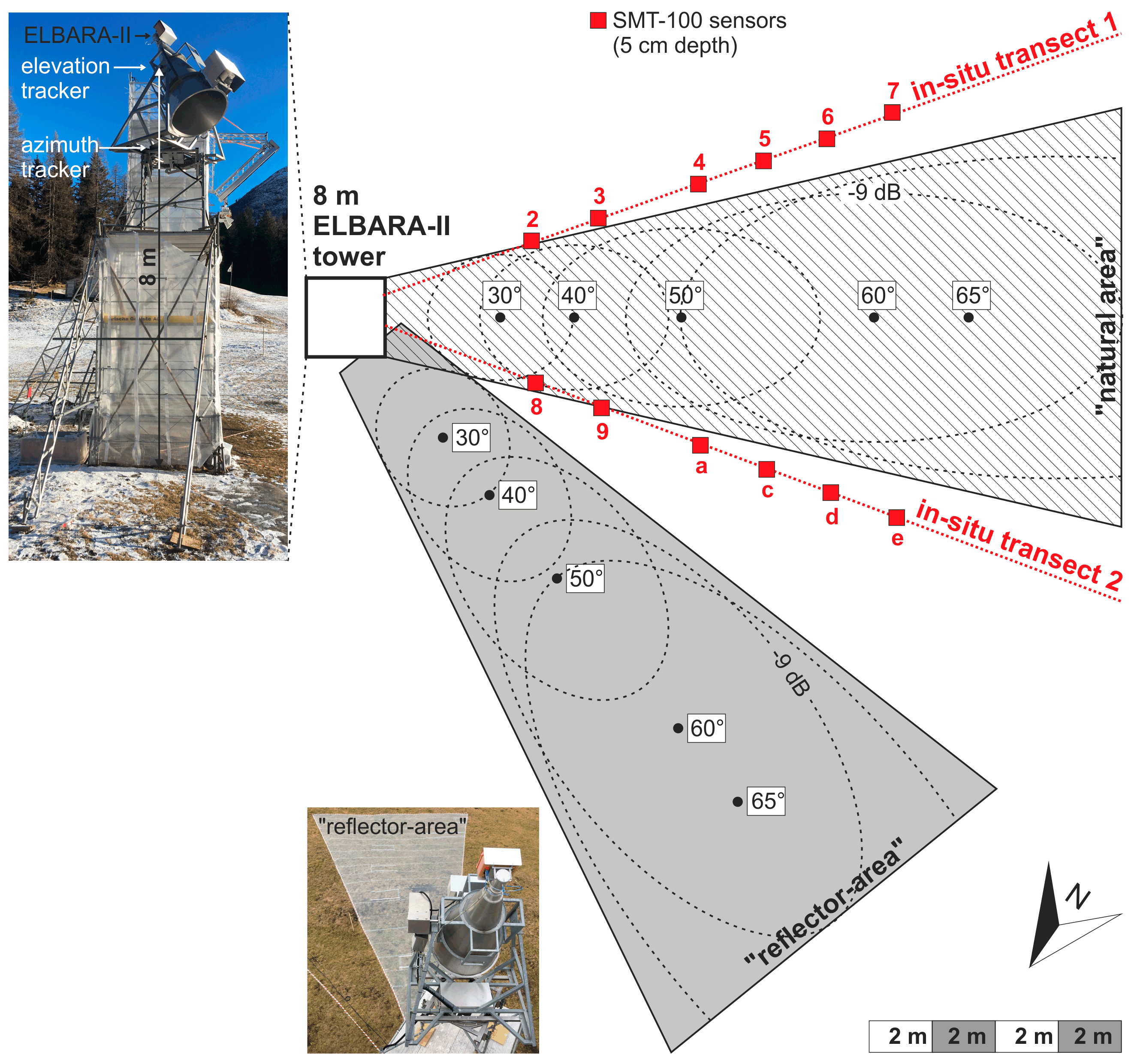
Temperatures and dielectric permittivities of the ground were measured every five minutes throughout the winter 2016/2017 campaign using an automated network of a dozen SMT-100 sensors. These sensors use a ring oscillator, in which a steep pulse, emitted by a line driver, travels along a closed transmission line buried in soil. The permittivity of the medium is computed through the travel time of the pulse. As indicated by red squares in Figure 1, SMT-100 sensors were located along two transects to capture in-situ permittivity and temperature of the ground at 5 cm depth with their spatial heterogeneity across the footprint areas of the radiometer. Detailed information on these in-situ measurements can be found in [22].
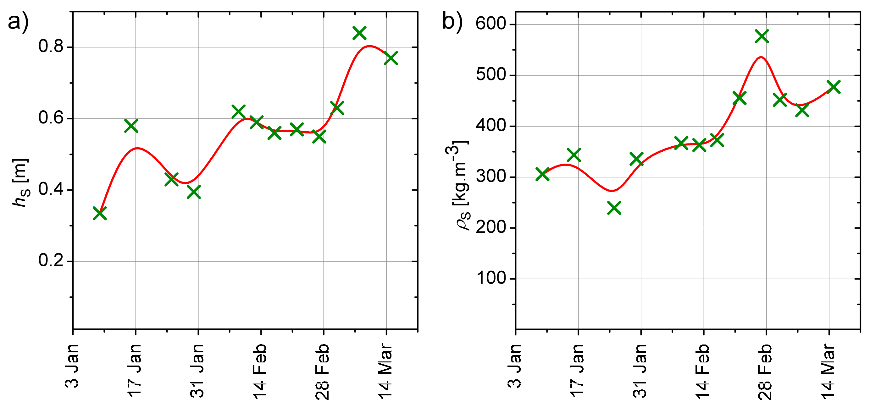
During the snow covered period, starting from 3 January 2017, regular snow depth profile measurements were performed manually. Snow height and mass-density were measured approximately once a week using a snow cutter with depth resolution of ≤10 cm. The green crosses in Figure 2a,b indicate measured and , where the latter represents average density of the bottom ~10 cm of the snowpack. Red lines are B-splines fitted to estimate temporal variations of and between sequential in-situ measurements and to reflect measurement uncertainties. The reason for showing the snow bottom-layer is that this is the most influential snowpack parameter on L-band emission of a ground covered with dry snow via its impedance matching and refractive effects as outlined in [24,27].
2.3. Radiometry Data
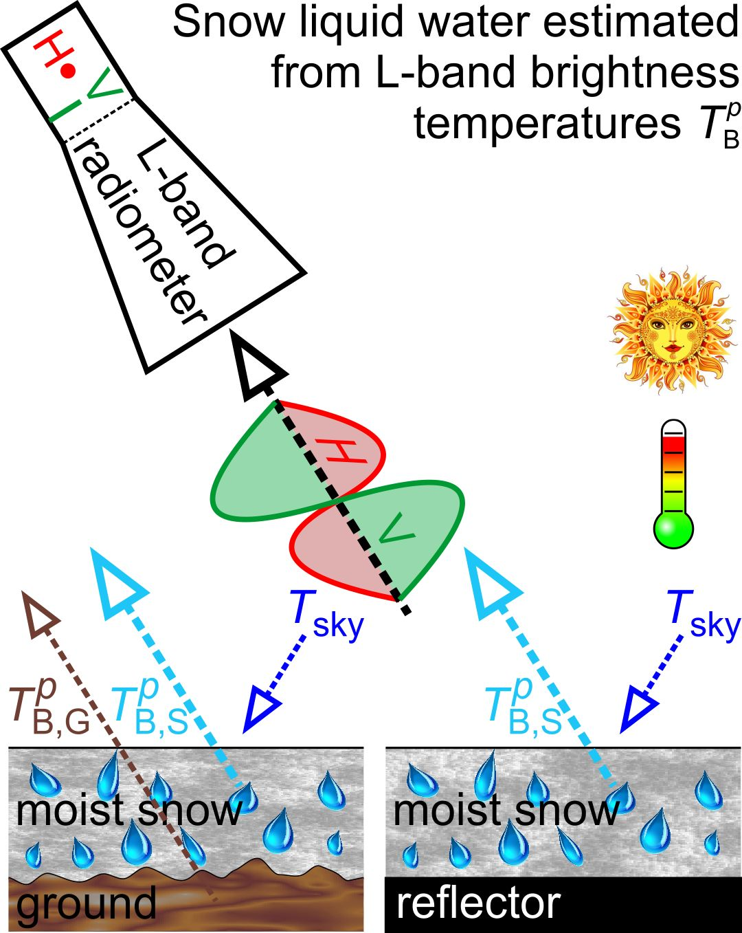
An ELBARA-II radiometer [29] was used to measure L-band brightness temperatures in the protected frequency band 1400 MHz–1427 MHz at both vertical and horizontal polarizations p = H, V. The instrument was mounted on an 8-meter tower and was equipped with tracking systems, allowing for automated observations of at discrete nadir angles and azimuth directions. The tracking systems were configured to perform sequential measurements along the azimuth direction of the “natural area” and the “reflector area”, with a metal mesh reflector placed on the ground, each with the eight nadir angles 30°, 35°,…, 65° (Figure 1). This measurement cycle was performed once an hour throughout the campaign. Sky measurements at were initiated manually during precipitation-free times, every two days when possible.
Calibrated L-band brightness temperatures measured over the either snow-free or snow-covered “natural area” (N) are indicated by . Measurements dominated by emissions originating from the “reflector area” are performed quasi-simultaneously. Together with the latter are used to extract radiance exclusively emitted by the “reflector area” (R) following the approach explained in [22]. The resultant represent, almost exclusively, the volume emission of the snow because of the very high reflectivity of the reflector covering the ground. As is well known, at L-band, the volume emission of seasonal snow is negligible under dry snow conditions [27,30]. However, as shown in Section 5 in [22], snow volume emission becomes significant for even slight amounts of snow liquid water. Accordingly, quasi-simultaneous and are essential to the research presented here, because it is the experimental key to separate snow volume emission from the overall emission of a snow covered natural ground.
3. Retrieval Approach
The general concept of the approach that is used to retrieve volumetric snow liquid water content is to optimally fit measurements to corresponding simulated (sim.) brightness temperatures . The numerically minimized cost function applied reads:
The concrete single parameter retrievals of snow liquid water content presented here are derived from measured of the “reflector area” (R), and derived from of the “natural area” (N). Furthermore, each type of retrieval is performed for three different “polarization modes” (first introduced and employed in [28]) RM = “H”, “V” including either observations at polarization p = H or V, and RM = “HV” using both polarizations. Furthermore, measured at nadir angles are used, implying that retrieved is an “effective” value of snow liquid water content representative of the entire area covered by the footprints observed at . The flowchart in Figure 3 illustrates the steps that are taken for achieving each of the two types of snow liquid water content retrievals and , plus the validation of the latter based on the former retrievals.
The denominator in Equation (1) assigns different weights to measurements , according to their uncertainty understood as the sum of the radiometer assembly’s (RMA) inherent uncertainty and the error imposed by non-thermal noise entering the antenna. The higher the value of the denominator in Equation (1), the lower the weight assigned to a measurement . In the case of ELBARA-II, the radiometer assembly’s uncertainty is [29,31]. The error caused by non-thermal radio frequency interference (RFI) is estimated from the non-Gaussianity of the probability density function (PDF) of the raw-data voltage sample that is associated with a given measurement . Highly RFI-corrupted (i.e., with coefficients of determination between the PDF of the measured raw-data voltage sample and a perfect Gaussian PDF) are excluded from retrievals. This RFI filtering and mitigation approach is explained in detail in Section 4.2 in [22].
Simulated used in the cost function defined in Equation (1) are computed with the L-band-specific emission model “LS—MEMLS”, as outlined in Section 5.1 in [22]. “LS—MEMLS” has previously been used successfully for retrievals of ground permittivity and snow bottom-layer density based on synthetic [24,28] and experimental [25] brightness temperatures. Additionally, the high sensitivity of simulated L-band brightness temperatures to snow liquid water content is demonstrated in Section 5.2 in [22], and is employed here for the retrieval of snow liquid water contents and using measured and , respectively.
The specific retrieval approach that is used to estimate snow liquid water content uses the single-layer version of “LS—MEMLS”. The corresponding equations used to express L-band of a rough ground covered with a homogeneous moist snowpack are found in Equations (13)–(21) in Section 5.1 in [22]. Through a global numerical minimization process based on tuning the value of the single retrieval parameter ( or ), the cost function in Equation (1) is minimized and the corresponding minimizing value of is taken as the retrieval result. The two slightly different configurations of the single-layer version of “LS—MEMLS” are used in the respective retrieval approaches that are employed to retrieve and from and . This is explained in Section 3.1 and Section 3.2. Before going any further, it is important to mention that the range of applicability for the snow liquid water retrieval method presented here is between . This is mainly because the penetration depth of L-band microwaves drops from >300 m in dry snow to ≈40 cm for wet snow with 5% snow liquid water content [14,32].
3.1. Approach Used to Retrieve from
As explained in Section 2.3, the exclusively respresent the volume emission of the snow. Knowing that the self-emission of dry snow at L-band is negligible [27,30], any increases in over the sky radiance , reflected by the metal reflector, is due to increased snow wetness. Therefore, retrievals , derived from , as measured over the “reflector area”, are considered as “reference” to validate snow liquid water content retrievals derived from measured over “natural area” (Figure 1). Accordingly, as shown in the left-handside of Figure 3, ground reflectivity is assumed, leading to the Kirchhoff coefficient of the ground (Equation (20) in [22]). Consequently, simulated (sim.) used in Equation (1) are necessarily independent of ground temperature , ground permittivity , and the HQN ground roughness parameters . Uncertainties of are estimated from the non-thermal RFI-induced errors of quasi-simultaneous brightness temperatures measured along the azimuth of the “natural area” and the “reflector area”. Gaussian error propagation is thereto employed using the equations provided in Section 4.4 in [22]. Furthermore, snow temperature is assumed as , which is physically reasomable for moist snow. On the other hand, the assumption made on is irrelevant for dry snow because of negligible snow emission in this case. Snow height and its mass density are represented by the corresponding in-situ measurements and , respectively, as shown in Figure 2. Accordingly, used as input in the single-layer version of “LS—MEMLS” are related to snow liquid water columns via .
3.2. Approach Used to Retrieve from
As indicated in Figure 3, retrievals are derived from measured over the “natural area” using a two-step approach. The first step consists of retrieving ground permittivity and snow mass density based on measurements . In this multi-angular two-parameter retrieval, the snowpack is formally assumed as dry (). The retrieval approach and its sensitivity to liquid water is outlined in detail in the companion paper [23]. The reader is further referred to [24,25,28], where a similar retrieval approach is comprehensively explained and employed for both synthetic and experimental data. However, it is once more emphasized that two-parameter retrievals that are based on measurements over the “natural area” are used as “pseudo-measurements” to retrieve from the same measurements . The second step consists of retrieving using the single-layer version of “LS—MEMLS” that includes snow liquid water to simulate . In contrast to Section 3.1, ground reflectivity is not assumed as here, and thus none of the Kirchhoff coefficients , , (Equation (20) in [22]) used to simulate is zero. Instead, the complete single layer version of “LS—MEMLS”, outlined in Section 5.1 in [22], is used. Ground temperatures are represented by the means of the in-situ measurements along the two transects (Section 2.2). Just as in the first retrieval step (to achieve the “pseudo-measurements” ), the HQN ground roughness parameters are assumed as = . Uncertainties caused by non-thermal RFI are estimated from the level of non-Gaussianity of PDFs associated with measurements following the approach explained in Section 4.2 in [22]. Furthermore, snow temperature is assumed as for the same reasons provided in Section 3.1, and snow heights are represented by the in-situ measurements shown in Figure 2a. The significance of the outlined two-step (first then ) retrieval of the three parameters lies in their independence from ancillary data such as ground permittivity and snow density.
4. Results and Discussion
4.1. Snow Wetness Retrieval Using
This section presents the retrieval of based on using the methodology presented in Section 3.1. Time series of retrievals are used in Section 4.2 in order to assess the meaningfulness of retrieved from measurements performed over natural snow-covered ground areas.
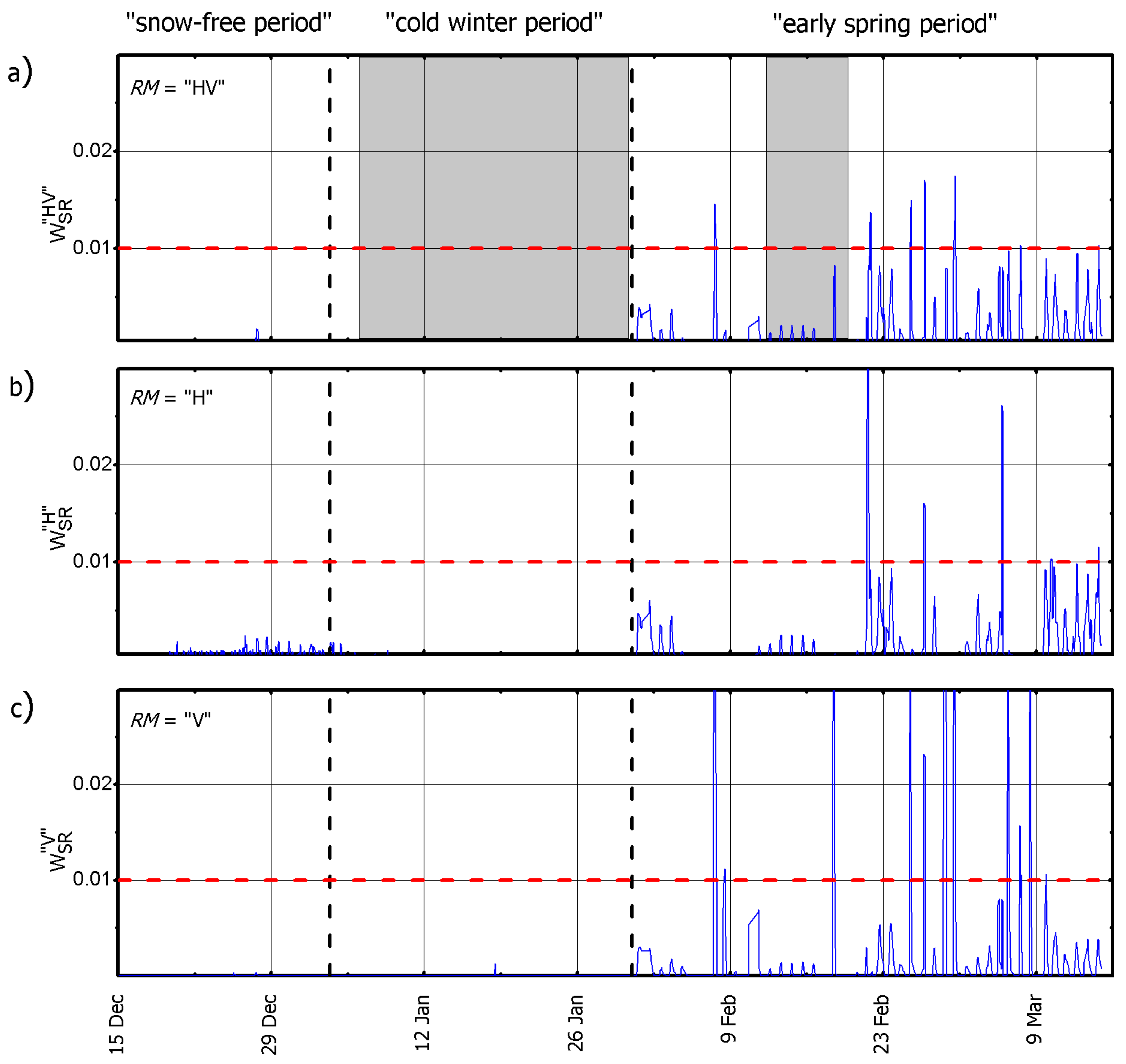
Figure 4a,b, and c contain the time series of volumetric liquid water content retrieval results for retrieval modes RM = “HV”, “H”, and “V”, respectively. Throughout the “snow-free period” (15 December 2016 to 3 January 2017), the retrievals for all three retrieval modes are virtually zero, which is, of course, expected in the absence of a snow cover. Nevertheless, occasional non-zero retrievals are observed for the “snow-free period”, especially for RM = “H”. To understand this, it is recalled that brightness temperatures are not directly measured, but computed using quasi-synchronous ELBARA-II measurements along the azimuth direction of the “natural area” and the “reflector area” (Figure 1). This results in the inclusion of small contributions from the surrounding areas with no metal reflector being placed on the ground. The computation method is comprehensively explained in Section 4.4 in [22]. Accordingly, during the “snow-free period”, soil liquid water content increases during the day as a result of exposure to direct sunlight and air temperatures above the freezing point. The impact of this increased soil moisture on L-band brightness temperatures can partly leak into through the non-idealities of its computation, causing it to slightly increase above its expected value , and consequently . However, with the onset of snow cover at the beginning of the “cold winter period”, diurnal thawing of the soil is inhibited by the thermal insulation of the snowpack.
During the “cold winter period” (3–30 January), when the snowpack is consistently dry, for all RMs is zero. At the beginning of the “early spring period” (1 February–15 March), the snowpack gradually becomes slightly moist, resulting in diurnal increases of with its maximum being reached in the afternoons but still limited to <0.01 m3m−3. The wettening of the snowpack, as a result of integral heat input over time and gradually increasing air temperature, continues over the rest of February until the end of the campaign. This results in the general increase of and also in the number of occurrences when its values are higher than the moist snow threshold, defined as (dashed horizontal lines).
Comparing in Figure 4b with in Figure 4c shows similar temporal patterns of water content retrievals that are almost identical among the two RMs. However, in some cases, the retrieval mode RM = “V” shows a higher sensitivity to variations in snow liquid water. This is the case, for example, during the period 7–11 February where (Figure 4c) reveals a series of distinct peaks, which do not show up in the contemporaneous retrievals (Figure 4b). However, higher sensitivity of retrievals achieved with RM = ”V” as compared to RM = “H” is consistent with the model-based sensitivity analysis of brightness temperatures with respect to snow liquid water column presented in [22]. As is shown in the Figure 10 in [22], at vertical polarization are increased more than at horizontal polarization for any given snow liquid water column . Thus, the stronger amplitudes of (and sometimes their exclusive occurrence between 7–11 February) as compared to those of during periods when snow becomes periodically moist during afternoon hours, corroborates the modeling result that are more sensitive than with respect to .
Figure 5a,b provide more details by means of zoomed-in views of Figure 4a showing in the periods from 12–20 February and 8–30 January, respectively. The corresponding air temperatures measured outside the ELBARA-II radiometer, as well as the recorded precipitation rates r, are shown. The retrieval graph in Figure 5a shows signs of the “early-spring snow” in that the snowpack is dry in the morning of each day, but as rises and the snowpack is periodically subject to more heat input from the Sun and atmosphere, the snowpack becomes slightly moist and gradually returns to its dry status overnight. Furthermore, the evolution of the diurnal increases in shows that the snowpack refreezing-time slightly increases over the first six days of the period shown in Figure 5a. While the snowpack completely refreezes a few hours before midnight on 12 and 13 February, refreezing takes all the way until midnight to occur from 15–17 February. The observed trend of gradually increasing time for snowpack refreezing to occur is the consequence of steadily increasing integral energy input over time. The peak of around noon on 18 January is coincident with the precipitation of moist snow or rain taking place at air temperatures . Accordingly, the noticeably high response of demonstrates the sensitivity of the snow liquid water retrieval to moist precipitation on dry snow.
A high correlation between and can be seen in Figure 5a showing that almost every time with , the retrieved snow liquid water is . This is true even for 17 February when at its peak is colder than the previous days. However, due to this temperature decrease, the snowpack becomes slightly moist and refreezes quickly. Nevertheless, it should be noted that the condition is not sufficient for . This becomes obvious, for example, in Figure 5b, which shows that is constantly zero, even though after 19 January, air temperature rises above the freezing point. However, when comparing with Figure 5a, we observe that these diurnal periods with are significantly shorter, and that preceding are also lower. Consequently, the resulting “time-integrated heat-inputs” in combination with the associated “history of snow-states” is not sufficient to warm the snow to its melting temperature and to overcome ice latent-heat [33] that is required to release a phase-change from frozen ice to liquid snow water. Furthermore, retrievals in Figure 5b during the first half of January show that dry snow precipitation (for ) does not increase snow liquid water.
Generally speaking, the snow-melt is expected to have a relationship with and its history so much so that some snow evolution models have attempted to express snow-melt rates as a function of air-temperature measured in terms of “degree-days” above freezing [34,35,36]. However, the “degree-days” factor method “implies an assumption of a constant relative contribution of each of the components of the heat balance equations to air temperature” [37]. Such components include, but are not limited to, energy input that is required to warm dry snow to the melting temperature and rate of heat-transfer through the snowpack [38]. In this respect, measurement-based information on interdependencies between and time synchronous micro-meteorological history can help to improve the calibration of snow evolution model parameters that are used to parameterize snow energy inputs, fluxes, and capacities.
At this point, it is worth mentioning that a snowpack does not necessarily become moist strictly top-down as a result of an energy-input from above. A moist snow-layer can form even underneath the dry snow surface under certain conditions. Such conditions are mainly related to clear-sky situations with strong radiation from the Sun, but with cold air temperatures. Under these conditions, downwelling short-wave solar radiation can penetrate the upper few centimeters of a dry snowpack only to become absorbed below the snow-surface. This results in an energy-input that is dissipated to a snow sub-surface layer, which ultimately causes the situation of a moist snow-layer underneath the dry surface snow.
In order to estimate the total amount of snow liquid water, retrieved volumetric liquid snow water contents are converted into snowpack liquid water columns, defined as . Recalling that are retrieved assuming a single-layered homogeneous snowpack (Section 3), can be estimated using the in-situ-measured snow height shown in Figure 2a.
Figure 6 shows for the same days during the “early spring period” as in Figure 5a with the blue line (left axis). The corresponding snowpack water column is masked over with the magenta line (right axis). It can be seen that essentially follows the same pattern as . This holds true for the entire snow-covered time of the campaign and all three RMs. Consequently, it can be said that the single-layer assumption made in the retrieval scheme (Section 3) does not cause artificial peaks in retrievals. Furthermore, estimates of the snow liquid water column are mainly important when radiation losses in the snowpack are of interest to investigate, for instance, radiation penetration depth at L-band, ground visibility through the snowpack, snow albedo, and so on.
The snow liquid water content retrievals shown in this section, together with the provided explanations, confirm that retrievals are tightly connected to the physical snowpack evolution throughout the “cold winter period” and the “early spring period”. Accordingly, the retrievals are highly trustworthy, implying that they are not caused by any kind of cohesion hidden in the retrieval scheme. When considering this, we consider retrievals derived from emitted from the “reflector area” as “references” for comparison with derived from measured over the “natural area”. This is both of high relevance and high importance because, as explained in Section 1, in-situ methods that facilitate the reliable assessment of the amount of snow liquid water at field scales, and even more so at larger spatial scales, are lacking to date.
4.2. Snow Wetness Retrieval Using
The methodology and results for snow liquid water content retrieval using brightness temperatures measured over the “reflector area” is covered thus far in Section 3.1 and Section 4.1. In this section, the snow liquid water content retrievals , achieved from , measured over the “natural area”, is presented and discussed using the methodology explained in Section 3.2 and summarized in Figure 3.
Figure 7a–c show the retrievals for the entire campaign from 15 December 2016–15 March 2017 and for retrieval modes RM = “HV”, “H”, and “V”, respectively. Naturally, the snow liquid water retrievals during the “snow-free period” are irrelevant. Nevertheless, from the retrieval point of view, it is ideally expected that m3m−3. Indeed, virtually zero snow liquid water content is retrieved for RM = “HV” (Figure 7a) and “H” (Figure 7b) in the absence of a snow cover. The only exception here are the considerably high and retrievals around 24 December, which are the result of rainfall and the consequential increase in ground permittivity. However, in contrast to and , the retrievals at RM = “V” (Figure 7c) are not zero during the “snow-free period” and follow a nearly-diurnal variation pattern. The reason for these meaningless retrievals lies in the “pseudo-measurements” retrieved in the first step that was applied before the retrieval of (see Section 3.2). As shown in Figure 6 in the companion paper [23], the snow density retrievals during the “snow-free period” are as high as , which, together with small daily fluctuations of , can result in non-zero and fluctuating . This is not the case for the other retrieval modes RM = “H” and “HV” because the associated “pseudo-measurements” during the “snow-free period” are considerably lower ( for RM = “HV” and “H”).
Throughout the “cold winter period” (3–30 January), starting from the onset of snow cover, the retrievals for all three RMs indicate very low values (<0.05 m3m−3). When comparing the retrievals (Figure 7) and (Figure 4) for the same RMs shows that both retrieval signatures indicate the “cold winter period” similarly. However, while the “reference” retrievals for RM = “HV” and “H” (Figure 4a,b, respectively) are consistently throughout the entire “cold winter period”, the corresponding quasi-simultaneous retrievals occasionally show noisy low non-zero values. This reflects the expected higher noise-level of as compared to retrievals, and is explained as follows:
- Brightness temperatures emitted exclusively from the “reflector area” are significantly more sensitive to low amounts of snow liquid water than brightness temperatures that are emitted from the “natural area”. This is demonstrated theoretically and experimentally in [22], and was the main reason for suggesting the use of retrievals as “references” to validate .
- are achieved from using a simple single parameter retrieval approach assuming ground reflectivity and using in-situ measured snow density (Figure 2b) as previous knowledge (Section 3.1). Accordingly, retrievals do not require the antecedent retrievals , as is the case in the two-step approach that is used to retrieve from (Section 3.2), implying that are not distorted by erroneous . The “pseudo-measurements” used in the first retrieval step are subject to errors introduced via snow liquid water content (Section 4.1 in [23]), spatially heterogeneous ground permittivity (Section 4.2 in [23]), and other types of geophysical noise [28].
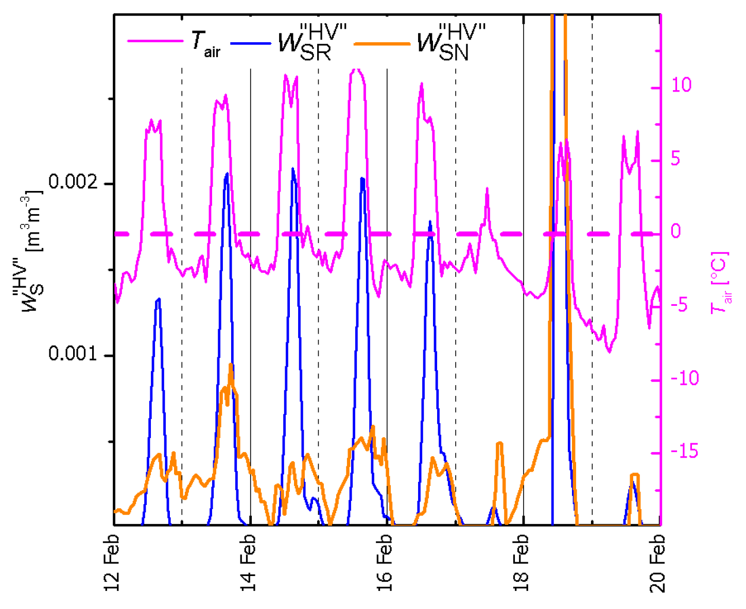
Despite these imposed uncertainties, retrievals successfully detect the occurrence of the first moist snow during the “early spring period” as one might expect from Figure 7. This proposition becomes more evident from the zoomed-in view in Figure 8 showing retrievals (orange) and (blue) for 12–20 February during the “early spring period” (the same period as shown in Figure 5a and Figure 6). Air temperature is indicated by the magenta line.
The shown retrievals performed for RM = “HV” follow almost exactly the same diurnal variation pattern as the corresponding “references” with virtually the same number of diurnal peaks and dips. Similarly, simultaneity between the and is also observed for RM = “H” and “V”. However, as can be expected, the shown are noisier than the “reference” retrievals , and their diurnal afternoon deflections are less pronounced, for the reasons stated in points 1 and 2 above. Despite the higher uncertainties, the still peak during afternoon hours and return to very low values (or even zero) through the night or in the early morning. This demonstrates that the sensitivity of retrieved with the two-step approach (Section 3.2) using measurements performed over the “natural area” (Figure 1) is still greater than the retrievals’ noise level, and is large enough to detect partial snow melting during afternoon hours and refreezing overnight.
The overall significance of these results is twofold. Firstly, dating the appearance of first moist-snow could become a valuable new data product accessible through passive L-band observations over natural snow covered ground, disregarding the current qualitative nature of retrievals. Secondly, the presented “reference” retrievals derived from L-band emission of the artificially prepared “reflector area” (Figure 1) represent a promising method for the validation of retrievals. Both of these instances are seen as relevant findings towards the full exploitation of L-band data measured over the cryosphere, which is made available through SMOS and SMAP missions, as well as other future L-band missions.
5. Summary and Conclusions
In the companion paper [23], which is a paralleled continuation of [22], we consider snow liquid water as a disturbance for retrieving mass density of dry snow and ground permittivity using the retrieval approach proposed in [24] and first validated in [25]. In the present paper, we take the reverse perspective, meaning that the high sensitivity of L-band brightness temperatures to snow liquid water, demonstrated in [22], is used for the retrieval of volumetric snow liquid water content from L-band radiometry. Snow moisture and based on multi-angular L-band and measured over the “reflector area” and the “natural area” are derived using two slightly different retrieval approaches. Retrievals are achieved through the inversion of the single-layer version of “LS—MEMLS”. As envisaged, retrievals behaved robustly and reliably, justifying the use of , as derived from , as “references” to assess the meaningfulness of retrievals . The latter are also achieved by the inversion of “LS—MEMLS”, although this involves two retrieval steps (first are retrieved, then ), and thus entails higher uncertainty and lower sensitivity.
The reliable representation of temporal variations in snow moisture is demonstrated for both types of quasi-simultaneous retrievals and . This is verified by the fact that both types of retrieval indicate a dry snowpack throughout the “cold winter period”, and synchronously detect the first occurrence of moist snow at the beginning of the “early spring period”. The clarity and level of detail that is found in the “reference” retrievals are exceptionally high. Furthermore, current methods that are used for the in-situ measurement of snow liquid water content are very limited, and, more importantly, suffer from low representativeness, limited spatial coverage, and prohibitively laborious measurement procedures. Hence, it is anticipated that interdependencies between derived from near distance L-band radiometry and time synchronous micro-meteorological history can help to improve the calibration of snow evolution model parameters that are used to parameterize snow energy inputs, -fluxes, and -capacities.
The recognition that , derived from measured over the “natural area”, can also successfully detect the snowpack’s wetness state, as well as the onset of “early-spring” snow, is another key finding of the presented study. The significance of successful retrievals lies in the fact that they are achieved using exclusively, without the need for in-situ measurements, such as ground permittivity or snow density. This opens up the possibility of using airborne or spaceborne L-band radiometry data to estimate snow liquid water. In other words, the potential for the exploitation of passive L-band radiometry to yield information on snow wetness as a new data product is demonstrated.
Nonetheless, there exist many challenges to further development of the proposed new retrieval approach to achieve its full potential. Its quantitative validation, particularly at large spatial scales, requires the advancement in in-situ snow moisture sensors and their widespread use. Field-capable electromagnetic resonator sensors, as used in [39], represent a reasonable option for in-situ measurement of the complex dielectric constant of snow, which is a sensitive proxy for volumetric snow liquid water content. Additionally, the conveyance of the proposed retrieval concept to spaceborne data is challenging and requires further fundamental research, as well as technical refinements in retrieval methods. The latter is particularly the case because, as yet, the spatial resolution of spaceborne L-band radiometers is typically low. Thus, their footprint areas often include complex combinations of mixed land cover, which needs to be taken into account in the forward modeling of brightness temperatures involved in the retrieval of snow moisture.
Acknowledgments
This paper was supported in part by the Swiss National Science Foundation under Grant 200021L_156111 /1, and in part by ESA within the framework of ESA’s SMOS ‘Expert Support Laboratory’ (ESL) for Level 2. Furthermore, we acknowledge the Forschungszentrum Jülich (FZJ) for providing the ELBARA-II radiometer funded via the German Helmholtz Association TERrestrial ENvironmental Observatories (TERENO) infrastructure project. We also acknowledge Christian Mätzler who provided valuable scientific inputs to the research presented. Furthermore, we thank Matthias Jaggi from the WSL Institute for Snow and Avalanche Research SLF for conducting in-situ snow characterization measurements, and Curtis Gautschi for editing the manuscript.
Author Contributions
Reza Naderpour and Mike Schwank conceived, designed, and performed the experiments in equal shares. Likewise, they contributed equally to the data analyses and the writing of the manuscript.
Conflicts of Interest
The authors declare no conflict of interest.
References
- Takala, M.; Luojus, K.; Pulliainen, J.; Derksen, C.; Lemmetyinen, J.; Kärnä, J.P.; Bojkov, B. Estimating northern hemisphere snow water equivalent for climate research through assimilation of space-borne radiometer data and ground-based measurements. Remote Sens. Environ. 2011, 115, 3517–3529. [Google Scholar] [CrossRef]
- Derksen, C.; Brown, R. Spring snow cover extent reductions in the 2008–2012 period exceeding climate model projections. Geophys. Res. Lett. 2012, 39, 19. [Google Scholar] [CrossRef]
- Mudryk, L.; Derksen, C.; Kushner, P.; Brown, R. Characterization of Northern Hemisphere snow water equivalent datasets, 1981–2010. J. Clim. 2015, 28, 8037–8051. [Google Scholar] [CrossRef]
- Barnett, T.P.; Adam, J.C.; Lettenmaier, D.P. Potential impacts of a warming climate on water availability in snow-dominated regions. Nature 2005, 438, 303–309. [Google Scholar] [CrossRef] [PubMed]
- Diffenbaugh, N.S.; Scherer, M.; Ashfaq, M. Response of snow-dependent hydrologic extremes to continued global warming. Nat. Clim. Chang. 2013, 3, 379. [Google Scholar] [CrossRef] [PubMed]
- Mankin, J.S.; Viviroli, D.; Singh, D.; Hoekstra, A.Y.; Diffenbaugh, N.S. The potential for snow to supply human water demand in the present and future. Environ. Res. Lett. 2015, 10, 114016. [Google Scholar] [CrossRef]
- Brun, E. Investigation on Wet-Snow Metamorphism in Respect of Liquid-Water Content. Ann. Glaciol. 1989, 13, 22–26. [Google Scholar] [CrossRef]
- Jiancheng, S.; Dozier, J.; Rott, H. Deriving snow liquid water content using C-band polarimetric SAR. In Proceedings of the 1993 Better Understanding of Earth Environment, International Geoscience and Remote Sensing Symposium, IGARSS ‘93, Tokyo, Japan, 18–21 August 1993; Volume 3, pp. 1038–1041. [Google Scholar]
- Mätzler, C. Thermal Microwave Radiation: Applications for Remote Sensing; IEE Electromagnetic Waves Series No. 52; The Institution of Engineering and Technology: London, UK, 2006. [Google Scholar]
- Stiles, W.H.; Ulaby, F.T. The active and passive microwave response to snow parameters: 1. Wetness. J. Geophys. Res. Oceans 1980, 85, 1037–1044. [Google Scholar] [CrossRef]
- Mätzler, C.; Schanda, E. Snow mapping with active microwave sensors. Int. J. Remote Sens. 1984, 5, 409–422. [Google Scholar] [CrossRef]
- Arslan, A.N.; Hallikainen, M.T.; Pulliainen, J.T. Investigating of snow wetness parameter using a two-phase backscattering model. IEEE Trans. Geosci. Remote Sens. 2005, 43, 1827–1833. [Google Scholar] [CrossRef]
- Kennedy, J.; Sakamoto, R. Passive microwave determinations of snow wetness factors. In Proceedings of the 4th International Symposium on Remote Sensing of Environment, Ann Arbor, MI, USA, 12–14 April 1966; pp. 161–171. [Google Scholar]
- Hofer, R.; Mätzler, C. Investigations on snow parameters by radiometry in the 3- to 60-mm wavelength region. J. Geophys. Res. 1980, 85, 453. [Google Scholar] [CrossRef]
- Schanda, E.; Matzler, C.; Kunzi, K. Microwave remote sensing of snow cover. Int. J. Remote Sens. 1983, 4, 149–158. [Google Scholar] [CrossRef]
- Matzler, C.; Strozzi, T.; Weise, T.; Floricioiu, D.-M.; Rott, H. Microwave snowpack studies made in the Austrian Alps during the SIR-C/X-SAR experiment. Int. J. Remote Sens. 1997, 18, 2505–2530. [Google Scholar] [CrossRef]
- Shi, J.; Dozier, J. Inferring snow wetness using C-band data from SIR-C’s polarimetric synthetic aperture radar. IEEE Trans. Geosci. Remote Sens. 1995, 33, 905–914. [Google Scholar]
- Sun, C.; Neale, C.M.; McDonnell, J.J. Snow wetness estimates of vegetated terrain from satellite passive microwave data. Hydrol. Process. 1996, 10, 1619–1628. [Google Scholar] [CrossRef]
- Stein, J.; Kane, D.L. Monitoring the unfrozen water content of soil and snow using time domain reflectometry. Water Resour. Res. 1983, 19, 1573–1584. [Google Scholar] [CrossRef]
- Schneebeli, M.; Davis, R. Time-Domain Reflectometry as a Method to Measure Snow Wetness and Density. In Proceedings of the International Snow Science Workshop, Beckenridge, Colorado Avalanche Information Centre, Denver, CO, USA, 4–8 October 1992; pp. 36–364. [Google Scholar]
- Schneebeli, M.; Coléou, C.; Touvier, F.; Lesaffre, B. Measurement of density and wetness in snow using time-domain reflectometry. Ann. Glaciol. 1998, 26, 69–72. [Google Scholar] [CrossRef]
- Naderpour, R.; Schwank, M.; Mätzler, C. Davos-Laret Remote Sensing Field Laboratory: 2016/2017 Winter Season L-Band Measurements Data-Processing and Analysis. Remote Sens. 2017, 9, 1185. [Google Scholar] [CrossRef]
- Schwank, M.; Naderpour, R. Snow Density and Ground Permittivity Retrieved from L-Band Radiometry: Melting Effects. Remote Sens. 2018, 10, 354. [Google Scholar]
- Schwank, M.; Mätzler, C.; Wiesmann, A.; Wegmüller, U.; Pulliainen, J.; Lemmetyinen, J.; Drusch, M. Snow Density and Ground Permittivity Retrieved from L-Band Radiometry: A Synthetic Analysis. IEEE J. Sel. Top. Appl. Earth Obs. Remote Sens. 2015, 8, 3833–3845. [Google Scholar] [CrossRef]
- Lemmetyinen, J.; Schwank, M.; Rautiainen, K.; Kontu, A.; Parkkinen, T.; Mätzler, C.; Roy, A. Snow density and ground permittivity retrieved from L-band radiometry: Application to experimental data. Remote Sens. Environ. 2016, 180, 377–391. [Google Scholar] [CrossRef]
- Roy, A.; Toose, P.; Williamson, M.; Rowlandson, T.; Derksen, C.; Royer, A.; Arnold, L. Response of L-Band brightness temperatures to freeze/thaw and snow dynamics in a prairie environment from ground-based radiometer measurements. Remote Sens. Environ. 2017, 191, 67–80. [Google Scholar] [CrossRef]
- Schwank, M.; Rautiainen, K.; Mätzler, C.; Stähli, M.; Lemmetyinen, J.; Pulliainen, J.; Drusch, M. Model for microwave emission of a snow-covered ground with focus on L band. Remote Sens. Environ. 2014, 154, 180–191. [Google Scholar] [CrossRef]
- Naderpour, R.; Schwank, M.; Mätzler, C.; Lemmetyinen, J.; Steffen, K. Snow Density and Ground Permittivity Retrieved From L-Band Radiometry: A Retrieval Sensitivity Analysis. IEEE J. Sel. Top. Appl. Earth Obs. Remote Sens. 2017, 10, 3148–3161. [Google Scholar] [CrossRef]
- Schwank, M.; Wiesmann, A.; Werner, C.; Mätzler, C.; Weber, D.; Murk, A.; Wegmüller, U. ELBARA II, An L-Band Radiometer System for Soil Moisture Research. Sensors 2010, 10, 584–612. [Google Scholar] [CrossRef] [PubMed]
- Wiesmann, A.; Mätzler, C. Microwave emission model of layered snowpacks. Remote Sens. Environ. 1999, 70, 307–316. [Google Scholar] [CrossRef]
- Schwank, M.; Wigneron, J.P.; Lopez-Baeza, E.; Völksch, I.; Mätzler, C.; Kerr, Y. L-Band Radiative Properties of Vine Vegetation at the SMOS Cal/Val Site MELBEX III. IEEE Trans. Geosci. Remote Sens. 2012, 50, 1587–1601. [Google Scholar] [CrossRef] [Green Version]
- Mätzler, C.; Aebischer, H.; Schanda, E. Microwave dielectric properties of surface snow. IEEE J. Ocean. Eng. 1984, 9, 366–371. [Google Scholar] [CrossRef]
- Pomeroy, J.; Brun, E. Physical properties of snow. In Snow Ecology: An Interdisciplinary Examination of Snow-Covered Ecosystems; Springer: Dordrecht, The Netherlands, 2001; pp. 45–126. [Google Scholar]
- Bergstroem, S. The development of a snow routine for the HBV-2 model. Hydrol. Res. 1975, 6, 73–92. [Google Scholar]
- Kuusisto, E. On the values and variability of degree-day melting factor in Finland. Hydrol. Res. 1980, 11, 235–242. [Google Scholar]
- Martinec, J.; Rango, A.; Major, E. The Snowmelt-Runoff Model (SRM) User’s Manual; NASA: Washington, DC, USA, 1983.
- Lang, H.; Braun, L. On the information content of air temperature in the context of snow melt estimation. IAHS Publ. 1990, 190, 347–354. [Google Scholar]
- Wilson, W.T. An outline of the thermodynamics of snow-melt. Eos Trans. Am. Geophys. Union 1941, 22, 182–195. [Google Scholar] [CrossRef]
- Mätzler, C. Microwave permittivity of dry snow. IEEE Trans. Geosci. Remote Sens. 1996, 34, 573–581. [Google Scholar] [CrossRef]
Figure 1.
Schematics of the Davos-Laret Remote Sensing Field Laboratory [22] during the winter 2016/17 campaign.
Figure 1.
Schematics of the Davos-Laret Remote Sensing Field Laboratory [22] during the winter 2016/17 campaign.

Figure 2.
(a) Measured snow height , and (b) density of the bottom ~10 cm of the snowpack. Snow melted down in the second half of March, and disappeared within ~10 days (see [22]).
Figure 2.
(a) Measured snow height , and (b) density of the bottom ~10 cm of the snowpack. Snow melted down in the second half of March, and disappeared within ~10 days (see [22]).

Figure 3.
Flowchart representing the approaches used to achieve “reference” retrievals of snow liquid water content from measured over the “reflector area” (a), and of snow liquid water content retrieved from measurements measured over the “natural area” (b). Retrieval approaches are under-laid in light gray; specific parameter values are under-laid in white.
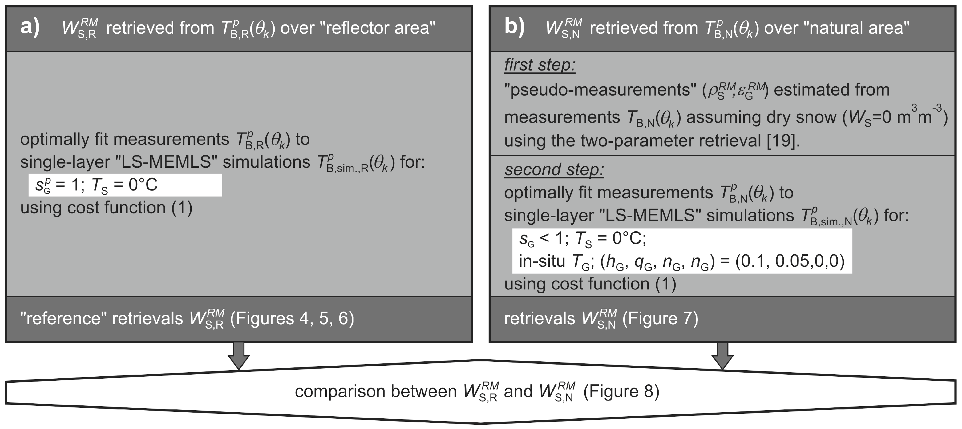
Figure 4.
Retrievals of snow liquid water content derived from for (a) RM = “HV”, (b) RM = “H”, and (c) RM = “V”, respectively. Light gray overlays indicate the zoomed-in view of shown in Figure 5.
Figure 4.
Retrievals of snow liquid water content derived from for (a) RM = “HV”, (b) RM = “H”, and (c) RM = “V”, respectively. Light gray overlays indicate the zoomed-in view of shown in Figure 5.

Figure 5.
Zoomed-in views of shown in Figure 4a for (a) 12–20 February during the “early-spring period”, and (b) 8–30 January during the “cold winter period”. Air temperatures are indicated by magenta lines; precipitation rates r are shown in the bottom panels.
Figure 5.
Zoomed-in views of shown in Figure 4a for (a) 12–20 February during the “early-spring period”, and (b) 8–30 January during the “cold winter period”. Air temperatures are indicated by magenta lines; precipitation rates r are shown in the bottom panels.
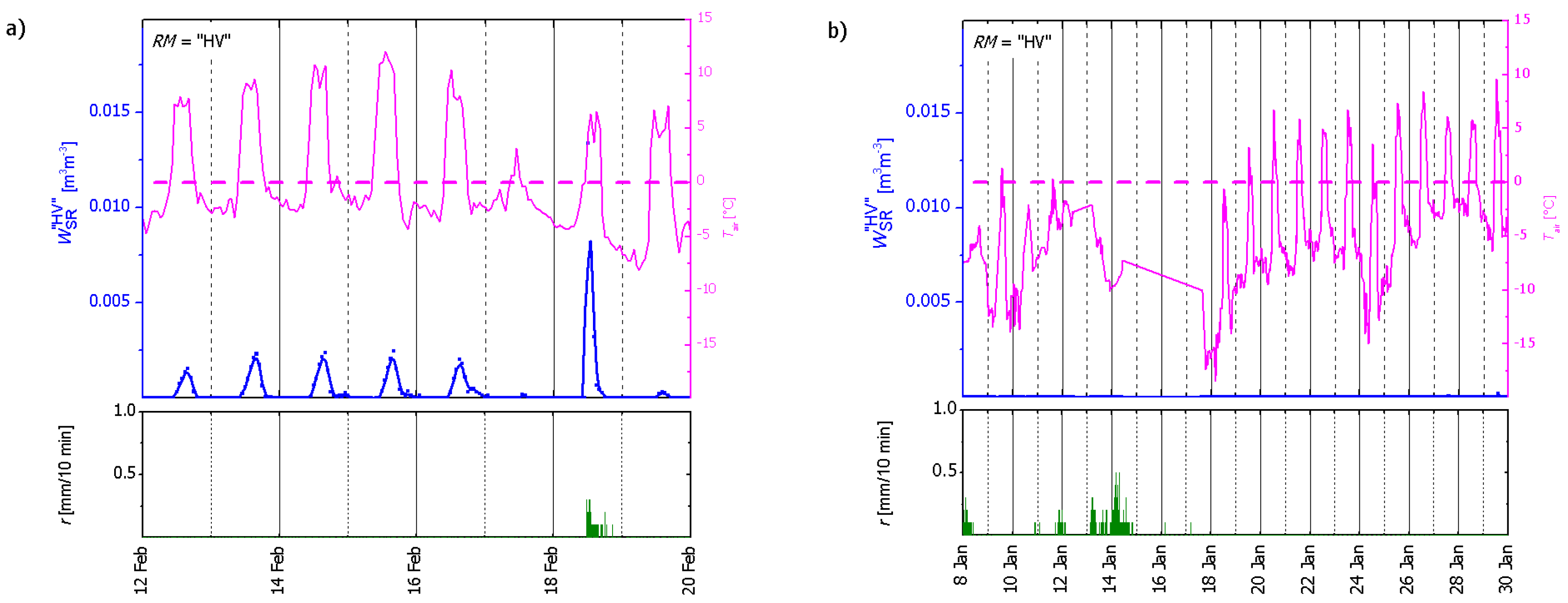
Figure 6.
Same snow liquid water content retrievals during the “early-spring period” as in Figure 5a (blue, left axes). Corresponding snow liquid water column (green, right axes) considering snow height , as shown in Figure 2a.
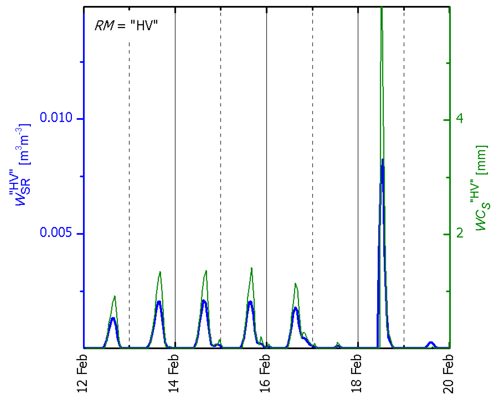
Figure 7.
(a–c) show snow liquid water retrievals using for RM = “HV”, “H”, and “V”, respectively. The retrievals are shown for the snow-covered period from 8 January to 15 March The horizontal dashed red lines indicate the threshold as the rough moist-snow approximation.
Figure 7.
(a–c) show snow liquid water retrievals using for RM = “HV”, “H”, and “V”, respectively. The retrievals are shown for the snow-covered period from 8 January to 15 March The horizontal dashed red lines indicate the threshold as the rough moist-snow approximation.
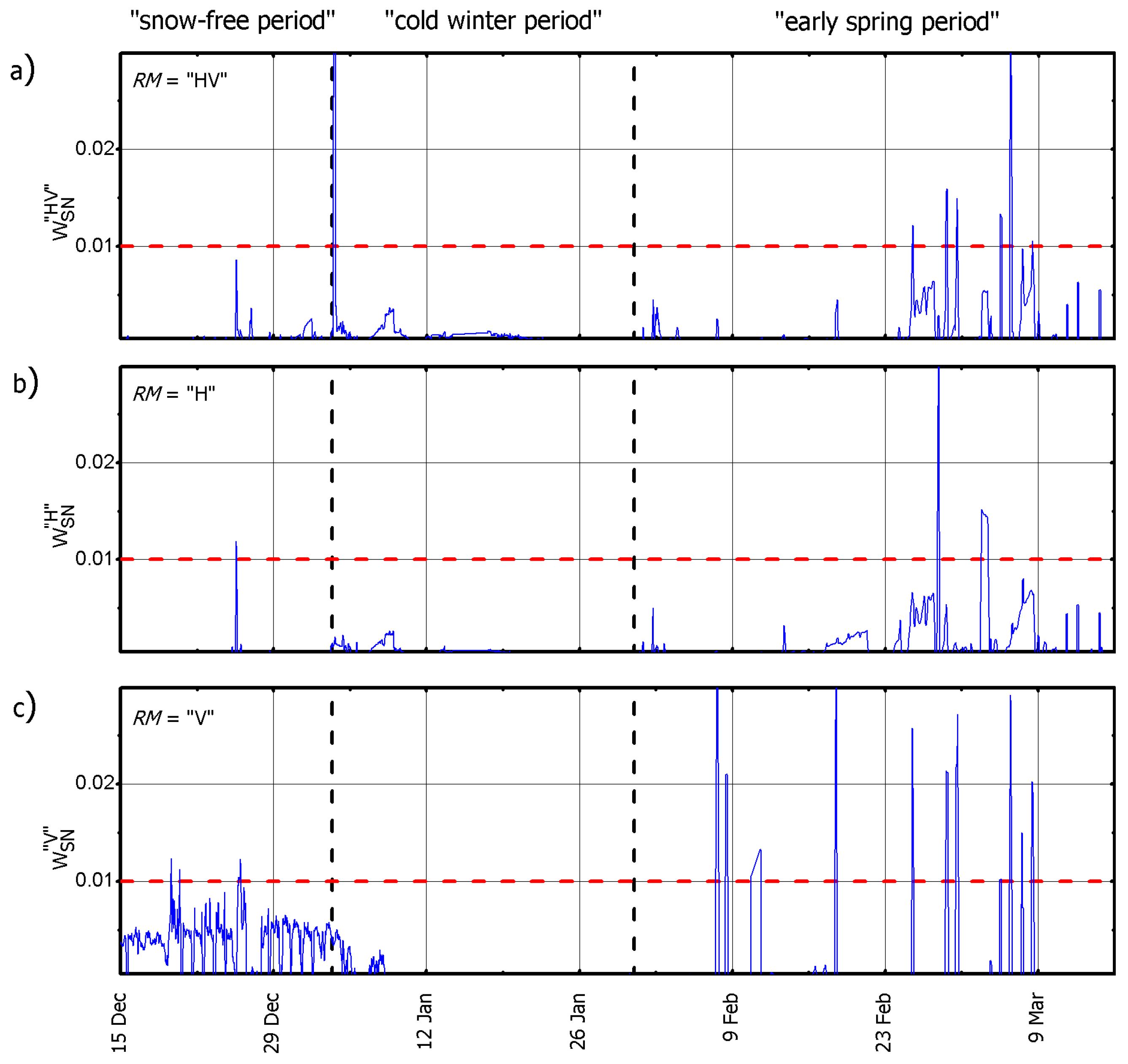
Figure 8.
The orange line indicates retrievals using from 12–20 February. The blue and magenta lines show the retrievals (Figure 5a) and the air temperature, respectively. It is evident that retrievals and “reference” retrievals are harmonized and undergo a similar diurnal variation pattern.
Figure 8.
The orange line indicates retrievals using from 12–20 February. The blue and magenta lines show the retrievals (Figure 5a) and the air temperature, respectively. It is evident that retrievals and “reference” retrievals are harmonized and undergo a similar diurnal variation pattern.

© 2018 by the authors. Licensee MDPI, Basel, Switzerland. This article is an open access article distributed under the terms and conditions of the Creative Commons Attribution (CC BY) license (http://creativecommons.org/licenses/by/4.0/).
Share and Cite
MDPI and ACS Style
Naderpour, R.; Schwank, M. Snow Wetness Retrieved from L-Band Radiometry. Remote Sens. 2018, 10, 359. https://doi.org/10.3390/rs10030359
AMA Style
Naderpour R, Schwank M. Snow Wetness Retrieved from L-Band Radiometry. Remote Sensing. 2018; 10(3):359. https://doi.org/10.3390/rs10030359
Chicago/Turabian StyleNaderpour, Reza, and Mike Schwank. 2018. "Snow Wetness Retrieved from L-Band Radiometry" Remote Sensing 10, no. 3: 359. https://doi.org/10.3390/rs10030359
Note that from the first issue of 2016, this journal uses article numbers instead of page numbers. See further details here.