1. Introduction
Forests occupy approximately 31% of the total land on Earth [
1]. Forests have tangible and intangible benefits that include biological resources, water conservation, climate regulation, and carbon dioxide reserves [
2]. These vital functions depend on forest health, which has been threatened by forest pests and diseases. It is very important to protect forest health from damage.
The Chinese 8th National Forest Inventory showed that China had 208 million hectares of forest: equal to 21.63% of the total country land area [
3]. The forest area ranks 5th worldwide, but the forest coverage rate and per capita area is small [
4]. Meanwhile, China is a country with a high rate of forest diseases and insect pests, with more than 200 kinds of pests and diseases seriously endangering the forests [
5]. One of the most serious forest pests is the pine caterpillar due to its wide occurrence [
6]. There are more than 30 species of pine caterpillars (
Dendrolimus spp.) worldwide and 27 of them can be found in China. Pine caterpillars mainly harm pine, cypress, and fir trees, and have caused great damage to forests in China [
7]. When pine caterpillars erupt in a large forest, they are hard to control and eliminate. They cause stunted trees and even tree death, and seriously endanger forest health [
7,
8]. Based on this, pine caterpillars have always been the key target of forest protection in China.
It is quite difficult to monitor and prevent forest diseases and insect pests, especially using traditional surveys, which are time consuming and cannot cover large areas. As manual surveys are hard to apply in thick forests, they often miss the best opportunities to control plagues [
9]. Fortunately, remote sensing can solve these problems. Through the development of remote sensing, it becomes possible to monitor forest plague rapidly in a big area [
10,
11,
12,
13,
14]. It is a unique technique to obtain the space and spectral information of forests and retrieve parameters. With remote sensing images, it has become quicker and cheaper to identify forest health situations when compared to traditional field surveys [
15,
16,
17]. Landsat data is advantageous for large areas of forest and for long-term monitoring. On one hand, Landsat has been obtaining images with seven bands since 1984, which makes it possible to study in a long time-series. On the other hand, Landsat data has a spatial resolution of 30 m, which is compatible with forest monitoring on a regional scale [
18,
19,
20].
Lots of researchers have studied forest diseases and insect pests through the remote sensing technique. In the early days, hard wood damage caused by pear thrip could be identified efficiently in a special Landsat image display, where RGB channels were inputted with the TM5/TM4 band ratio, the TM5 band, and the TM3 band individually [
21]. The SWIR/NIR (Short Wave Infrared/Near Infrared) ratio of Landsat was found suitable for monitoring deciduous and coniferous forests, while the broadleaf forest was monitored by the NDVI (Normalized Difference Vegetation Index) from the Landsat data [
22]. For the Landsat data, the ratio of the TM4 and TM3 bands was found in negative correlation with a canopy cover of a damaged pine tree in the study of blight damage to a Japanese red pine forest [
23]. The TM5/TM4 band ratio was found appropriate for monitoring low-density forests while the TM4/TM3 band ratio was suitable for high-density forests in a study of Chinese masson pine damaged by pine caterpillars [
24,
25]. Recently, the spatiotemporal patterns of the mountain pine beetle and western budworm were successful in mapping tree mortality with Landsat data in a long time-series from 1984 to 2012, aerial detection survey (ADS) data from 1970 to 2012, and multi-data forest inventory data across the Pacific Northwest Region, USA [
26]. For constructing a general continuous model to assess broadleaf forest defoliation by gypsy moth, it proved feasible to apply a logistic regression model with a sensitive vegetation index, the normalized difference infrared index (NDII) [
27].
Nowadays, with the progress of remote sensing technology and the availability of satellite sources, higher spatial and spectral data can be applied. This has promoted deep research into image texture, and finer spectral features [
28,
29,
30,
31,
32]. As a result, monitoring and estimating forest damage by diseases and insect pests are becoming more precise and timely. However, most researchers have concentrated on the identification, classification, and assessment for forest damage with finer vegetation indexes and models [
33,
34,
35,
36,
37]. There is still little research on the prediction of damage with the change of climate and other factors. In the context of global warming, studying the effects of climate on insect pests and predicting the occurrence of forest pests in future would be helpful for forest management and defense against forest plagues [
38].
This paper aims to assess and predict the damage of large man-made pine forests (Pinus tabulaeformis) by pine caterpillar (D. tabulaeformis) using Landsat data in a long time-series based on vegetation index in West Liaoning Province, China. The mechanisms of meteorological and topographical effects on the damage were studied. Furthermore, prediction models were constructed to forecast yearly plague situations temporally for the whole study region, and spatially for special pine positions. This paper attempts to establish the quantitative relationship between the degree of damage to pine trees and the influence factors of the pine caterpillar. This will provide forestry managers with evidence of how the pine caterpillar outbreak occurs and where could it outbreak severely, which could prevent the damage and reduce forest loss.
2. Materials and Methods
2.1. Study Area and Pine Caterpillar
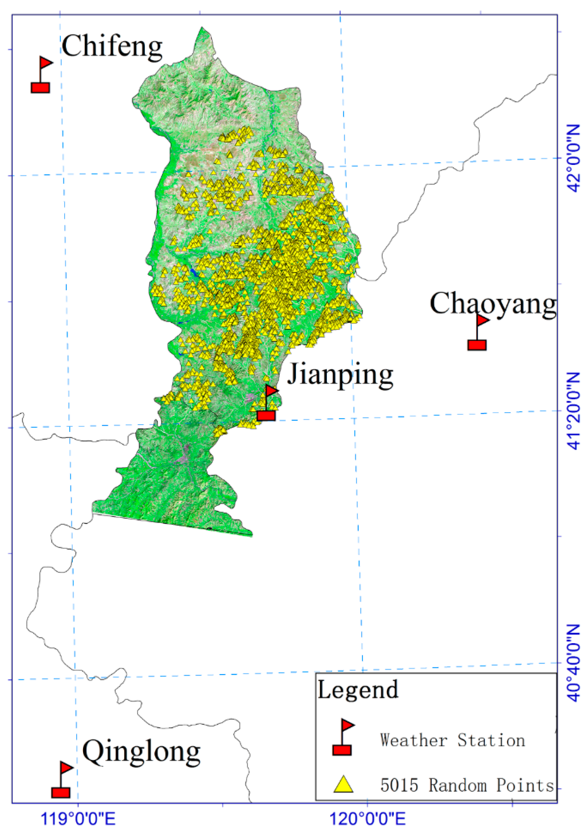
This study was carried out in Jianping county and the northern part of Lingyuan city, Western Liaoning Province, China (41°3′–42°22′N, 119°4′–120°4′E), as shown in
Figure 1. The altitude is around 300 to 1000 m. The terrain is flat and the slope is mainly under 30 degrees. Its climate zone transitions from a warm temperate semi-humid to semi-arid temperate zone, average precipitation ranges from 400 to 700 mm per year, and the average annual air temperature ranges from 6 to 10 degrees Celsius. In the study region, large man-made pine forests (
P. tabulaeformis) of about 686 km
2 are grown [
39]. The pine forests have been damaged by pine caterpillar (
D. tabulaeformis). The local forest protection station has been surveying, monitoring, and controlling the insect pest from 1983, as recorded.
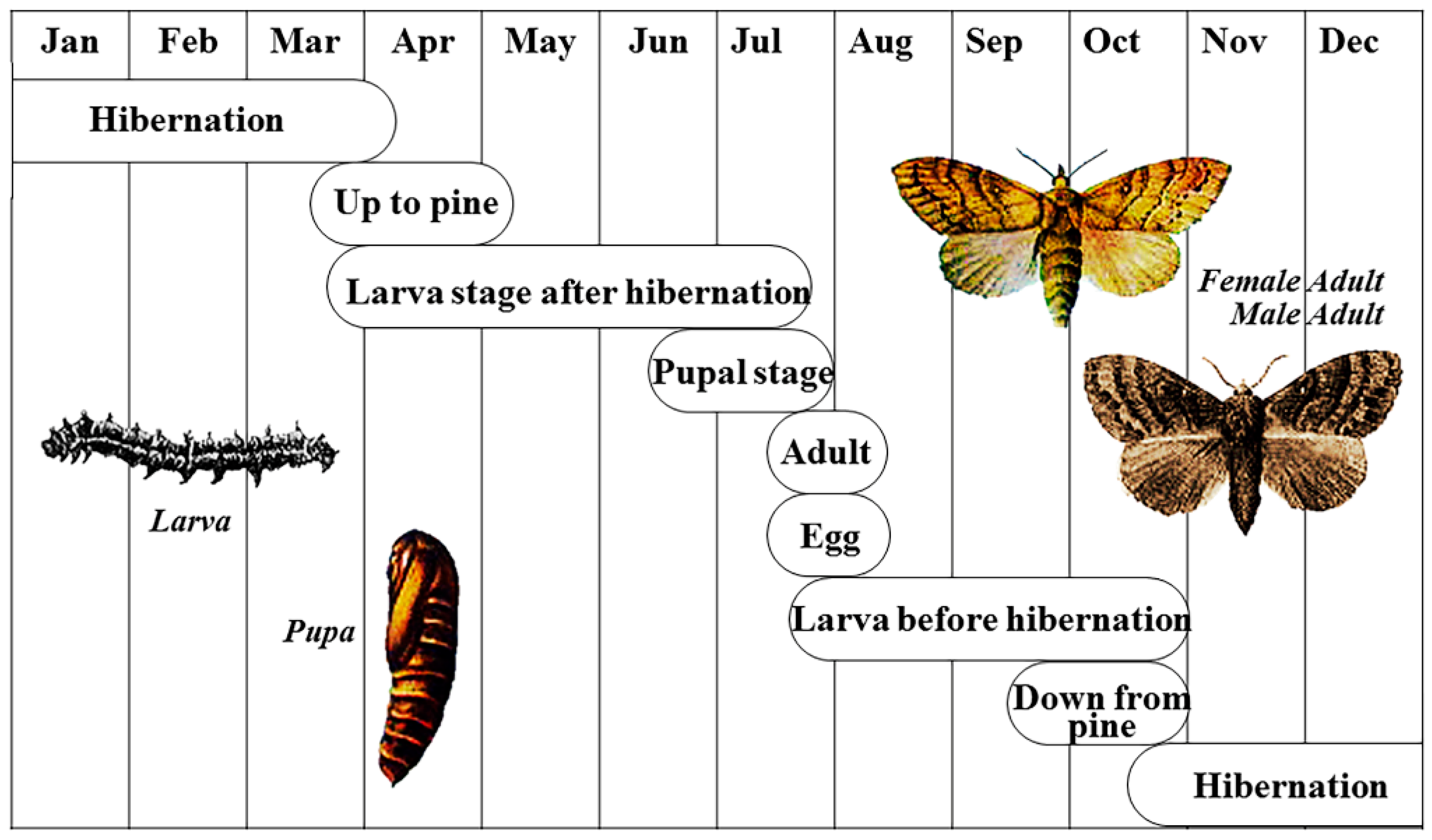
To predict the defoliation damage, knowledge of the life cycle and effective factors of the pest is necessary. The caterpillar is the main leaf-feeding pest to
P. tabulaeformis and its appetite for pine needles is enormous. This insect produces only one generation annually in the study area.
Figure 2 shows the life history of the insect. From March to May, this insect climbs back to the tree and eats needles after hibernation. From June to July, it eats the needles most heavily—about 70% of all needles eaten at its larval stage [
40]. From July to August, the big larvae turn to pupae and adults, and the insect stops damaging pine trees temporarily. Post adulthood, new eggs of the insect hatch larvae of a new generation from August to September. Then, before November, new larvae eat some of the pine needles—about 4.4% of all eating at its larval stage [
40]. Many environmental factors can affect the insect and the degree of damage such as forest terrain (slope and aspect), weather (sunshine duration, temperature, and rainfall), tree age, branch number, crown width, and density of the forest [
40].
2.2. Field Data
Nineteen field sample plots in pine forests were built from 2013 to 2016, and their defoliations were investigated in August 2016. Their degrees of damage were different. Four plots (blue rectangles in
Figure 1) were almost all healthy trees, others (yellow rectangles) were injured moderately and seriously by the caterpillar. The caterpillar was just propagating to the healthy plots from the injured in 2016. Each plot was in a 30 × 30 m
2 rectangular shape with about 100 pine trees distributed within. The defoliation ratio for each plot was calculated with sample trees distributed in four corners and the center of each plot. The defoliations of over 10 trees were estimated by the technicians of the local forest protection station for each plot, and the plot defoliation ratio was weighted by every tree’s DBH (Diameter at Breast Height) to obtain the plot average defoliation.
2.3. Landsat Data
Landsat data is suitable for the study of large forests as it provides a medium spatial resolution of 30 m, and six channels ranging from the visual band to the short wave infrared band. Furthermore, it has kept good time continuity since 1984, which was fitting for the long time-series study. The summer time, August and September, is the best period to monitor the damage [
41]; Landsat images with low cloud cover from August and September were downloaded as the study data from 1984 to 2016, covering the study area (WRS PATH = 121, WRS ROW = 31). There was a lack of images without cloud in August and September of 1987, 1988, 2005, and 2013, so in total, 29 years were studied from 1984 to 2016. Spring images with good quality were also downloaded at intervals of 3–5 years to update the range of pine forests. As the data spanned 32 years from 1984 to 2016, the region and age change of the pine trees was considered. All Landsat images used are shown in
Table 1 and were downloaded from the USGS Global Visualization Viewer (glovis.usgs.gov). To obtain accurate reflectance value on the image, radiometric calibration and FLAASH (Fast Line-of-sight Atmospheric Analysis of Spectral Hypercubes) atmospheric correction were progressed for each image [
42]. Additionally, geometric correction was progressed for a good consistency of image space position. The Landsat ETM+ images suffering a failure of Scan Line Correction (SLC-off) were corrected with SLC Gap-Filled Products Phase One Methodology [
43,
44]. Considering the terrain of the study region was flat, topographic correction was not carried out for the data.
After preprocessing, regions of evergreen forest were extracted with the spring image using the Normalized Difference Vegetation Index (NDVI) threshold (
Table 1). The NDVI threshold was determined by searching evergreen forests all over the colored spring image and finding the minimal NDVI value around the evergreen forests. This progress was requested to avoid mixing pixels on the forest boundary. The forest extracted was pure without mixing other objects.
More than 90% of evergreen forests belonged to
P. tabulaeformis in the study area according to local forest survey data [
41]. However, it was difficult to recognize
P. tabulaeformis from other local evergreen trees such as cypress and
P. sylvestris. Therefore, the evergreen forests extracted were assumed to be the pine forest (
P. tabulaeformis) and the range respected the pine range in the study. Then, the summer images were clipped with the pine range to obtain pine images of each year to study.
2.4. Meteorological and Other Data
Meteorological data was downloaded from China Meteorological Data Sharing Service System (data.cma.cn). Daily mean temperature, monthly rainfall, and monthly sunshine duration from 1979 to 2015 from four ground meteorological stations (Chifeng, Qinglong, Jianping, and Chaoyang) around the study area were downloaded specifically. The locations of the four meteorological stations are shown in
Figure 3. The time period from 1 August to 31 July of the next year was chosen as the effective duration for one generation of the caterpillar as every August is the beginning of a new generation according to the life cycle. The three meteorological parameters mentioned before were studied as the pine caterpillar is affected by temperature, rainfall, and sunshine duration [
40]. Second order inverse distance weighting interpolation (IDW) was applied to obtain the meteorological raster data of the study area by the four stations. The resolution of the interpolation raster equaled 30 m in accordance with the Landsat spatial resolution.
The Digital Elevation Model (DEM) data of the study was downloaded from Geospatial Data Cloud (gscloud.cn). The data were the product of ASTER GDEM V2 and offered a spatial resolution of 30 m. The slope and aspect raster data of the study region were calculated by the DEM given that the slope and aspect can affect the pine caterpillar [
45].
Furthermore, local survey records were offered by the Forest Protection Station of Jianping country including the caterpillar occurrence schedule, density, and average degree of damage investigated by manual evaluation from 1985 to 2013.
2.5. Inversion of Pine Foliage Remaining Ratio through Vegetation Index
Lots of research in forest health and defoliation detection have proved the validity of the Vegetation Index (VI). Different VIs perform different from site to site [
46]. To distinguish the light and severe conifer damage, the SWIR/NIR ratio was better than the NDVI, and for the broadleaf forest, NDVI was more suitable for monitoring with Landsat data [
22]. For detecting gypsy moth defoliation in the oak-dominated forest, the NDVI from the MODIS time-series was well applied [
29]. Recently, the NDII was proved fitted for inverting the broadleaf defoliation in a continuous way with Landsat data [
27].
To accurately indicate the damage of pine forests, several VIs were tested to find the best option. VIs were regressed with the foliage remaining ratio instead of the defoliation ratio because the forest on the image showed the spectral information of the foliage remaining directly. According to our summer field survey from 2013 to 2016, the caterpillar made the remaining needles turn brown and dry for damaged pine trees, in addition to a lot of defoliation. Obvious differences in color and water content existed between the healthy trees and the damaged ones. Although previous research [
41] showed that the NIR/Red Ratio Vegetation Index (RVI) had the ability to identify the degree of pine damage by the caterpillar, only NIR and Red channels are involved in the RVI. The RVI had not taken full advantage of the Landsat data as its SWIR channels were sensitive to plant water content. Therefore, in this paper, SWIR bands were added to construct VIs and their identity effects compared.
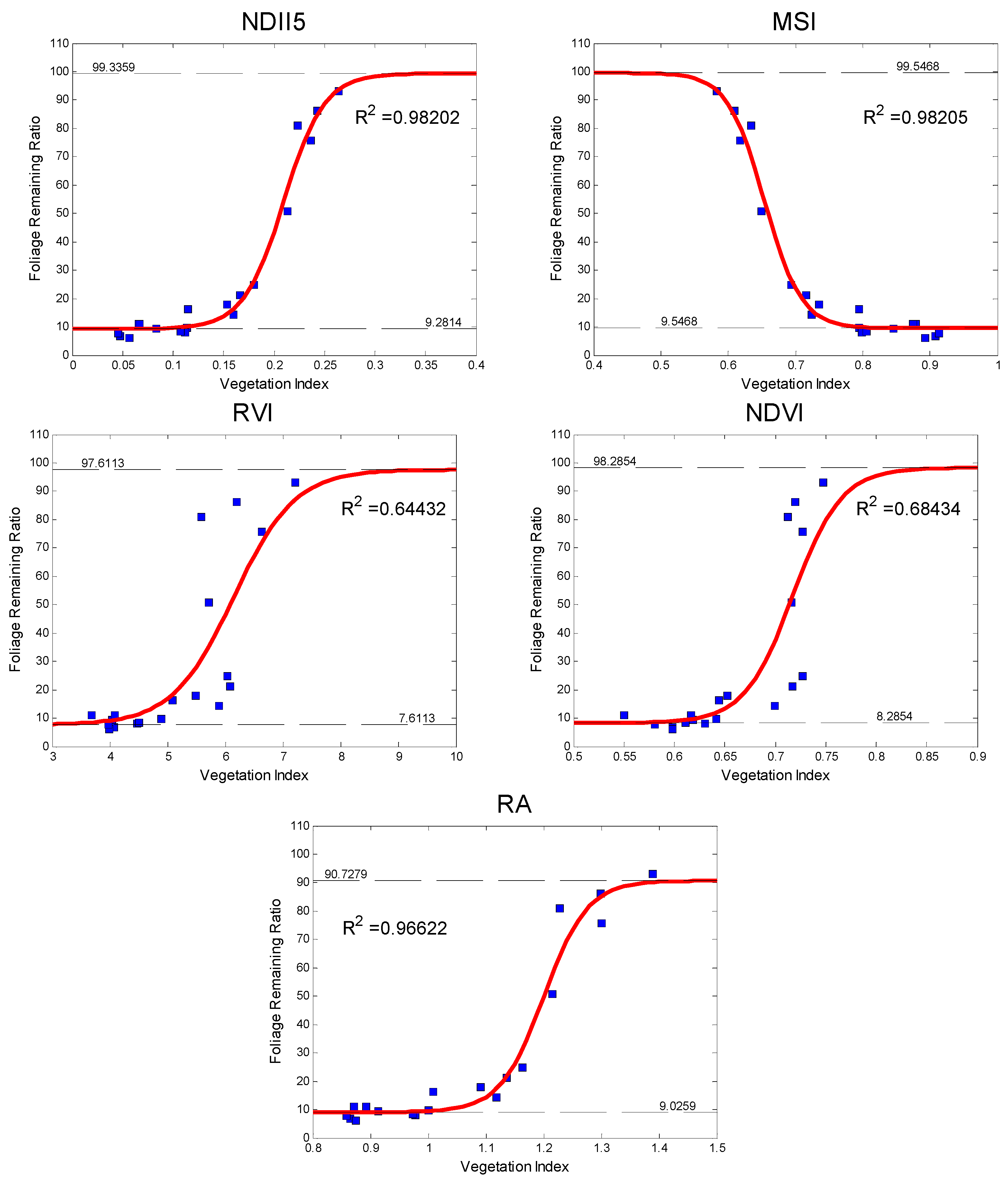
Five vegetation indexes, RVI, NDVI, NDII5 (Normalized Difference Infrared Index of 5th band, ), RA (Reflectance Absorption Index, ), and MSI (Moisture Stress Index, TM5/TM7) were tested. Their relevance with foliage remaining ratio of pine trees were calculated to select the best one. The detailed process was as followed.
First, five VI raster images were calculated from the Landsat 8 OLI image of 26 August 2016. The image range covered all 19 field plots. Their locations are shown in
Figure 1. These 19 plots included different statues of foliage remaining and could represent different degrees of damage by the pine caterpillar in the study region.
Second, the VI raster images were resampled from 30 m to 1 m in spatial resolution. Then, for each VI, the average value for each plot was obtained by averaging the VI values of all pixels inside each plot as the pixel size of the Landsat image was the same as the size of the plot. One pixel on the image could not fit one sample plot perfectly well. Averaging the VI value by the area ratio was a compromise method we used.
Third, the foliage remaining ratio of each plot was inverted by the plot average defoliation ratios. Fourth, for each VI, a scatter diagram of the average VI and foliage remaining ratio for each plot was drawn and regressed with a special proper regression function.
Fifth, according to the distribution of points on the scatter diagram, the correlation of regression function, the dynamic range and saturation effect for each VI [
47], the best VI could be selected. Furthermore, it inverted the foliage remaining ratio by the best-fitted function. The foliage remaining ratios of all pine forests could be calculated in a long time-series.
As a result, the distribution maps of the pine foliage remaining ratio for the study region across the whole 29 years could be obtained and the damage changes could be quantified year by year. By comparing the results to historical survey records from the Forest Protection Station, the reliability of the inverted results could be evaluated.
2.6. Choosing the Best Meteorological Factors
Under the constant condition of forest characters, insect pests are mainly affected by weather and climate. There are three main meteorological factors: temperature, rainfall, and sunshine duration [
40]. The key to selecting the best meteorological factors is to determine the periods of meteorological factors. Therefore, candidate meteorological factors in different periods were first enumerated as variables. Then, the correlation analysis of the converted foliage remaining ratio (from
Section 2.5) and meteorological variables was done for all years to select the best meteorological variables.
In this paper, two prediction models were constructed in a temporal scale and in spatial-temporal scale, respectively, so different meteorological variables were chosen for each.
According to the life history of the caterpillar (
Figure 2), it is in hibernation from November to next March. Therefore, one generation could be divided into two hazard phases. One phase is from August to October when the insect grows into a moth and gives birth to a new generation and the new larvae appear before hibernation. In this period, the moth has migratory capacity and the new larvae eat few needles, accounting for about 30% of total capacity [
40]. The second phase is from the following April to July when the insect larvae climb back to the pine tree and eat the needles after hibernation. During this period, the larvae cannot migrate, but focus on eating, so about 70% of needles of total capacity eaten by larvae are consumed.
As insect characters are different between these two phases, it is necessary to consider meteorological factors at each period respectively. Therefore, the rainfall and sunshine in the two periods and their sum were taken as candidate variables. Furthermore, the rainfall in October was also taken as a candidate variable as it affects whether the caterpillar can find dry soil to hibernate safely [
48]. Significant rainfall in October made the soil too wet for the caterpillar to hibernate.
For the temperature factor, the accumulated temperature of the daily temperature above 6 °C in one generation from August to the following July was taken as a candidate variable as the lowest temperature is about 6 °C for the pine caterpillar to live. Insect development requires a certain amount of cumulated daily temperature which affects the occurrence of the caterpillar [
49]. According to the daily temperature records from weather stations, the annual date when daily temperature was less than 6 °C was from the end of October to the beginning of April of the next year, which coincided with the hibernation date of the pine caterpillar. Therefore, the accumulated temperature of daily temperature above 6 °C was taken as a candidate variable, which was the active accumulated temperature for the pine caterpillar in meteorology.
Aside from spatial scale, the weak migratory ability of the caterpillar needs to be considered. The distribution of the pine caterpillar in the study region is the result of the long-time climate. Therefore, the average values of the last five years were added for the three kinds of meteorological factors as candidate variables. For example, for 2000, its average of the last five years was counted from 1986 to 2000. Five years could represent a long-time climate according to previous research [
41].
On a temporal scale, the occurrence of plague in a single year is only related to the weather condition of that year, so we did not apply the five years’ average in the temporal prediction model.
2.7. Prediction in Temporal Scale
Based on the inverted result of pine foliage remaining ratios for 29 years, a regular change of pine damage was found. This paper attempted to achieve a temporal prediction model for the whole study area. The occurrence of the caterpillar was affected by the meteorological change. Therefore, a correlation analysis was made between the meteorological factors and average plague degree (the foliage remaining ratio) for the whole region in corresponding years. Then, the regression function of the average foliage remaining ratio could be obtained to predict the annual plague degree in future.
Specifically, annual weather data was first counted from one meteorological site (Jianping) as the general weather data for the whole study area as the other three sites were out of the study region and only the Jianping site could represent the study area. The weather data counted included three factors:
Temperature. Only the active accumulated temperature in every generation of the caterpillar was considered as a variable (last August to July, >6 °C).
Sunshine duration. Three periods were taken as the candidate variables. These were the durations before the hibernation (last August to last October), after the hibernation (April to July), and the sum of both (last August to last October and April to July).
Rainfall. Four periods were taken as the candidate variables. Three of them were the same as the Sunshine duration, the fourth was one month of last October.
For each kind of meteorological factor, the variable with the highest correlation with the average foliage remaining ratio was taken as the best. The average foliage remaining ratio for the whole study area was weighted by the area of pine. After choosing the best variables, a linear regression function was constructed with them in the method of least squares to convert the foliage remaining. Its specific equation was as followed:
where the parameters a, b, c, and d are the constant coefficients; Temp means the active accumulated temperature; Rain means the best variable in four candidate variables of rainfall; and Sun means the best variable in three candidate variables of Sunshine duration.
Before this paper was finished, the weather data of 2016 year had not yet been updated on the China Meteorological Data Sharing System. Therefore, 2016 could not put into the analysis, so only 28 years were analyzed. For a single temporal scale, it was hard to construct an accurate model to predict the occurrence of the caterpillar due to four reasons:
The sample size was limited as there were only 28 samples for 28 years in the temporal scale.
The occurrence of forest pest had spatial characteristics as the insect could migrate with the change in climate.
For a big study area, the weather was multivariate and complicated. Different spatial locations had different meteorological conditions. It was not accurate to use the meteorological data of one meteorological site (Jianping) to represent the average of the whole study region.
Topographical and other factors could also affect the occurrence of the caterpillar except for the meteorology; however, they could not participate in the temporal prediction of damage.
2.8. Prediction in Spatiotemporal Scale
To predict the occurrence of the caterpillar in the whole study area accurately, it was necessary to extend from a temporal scale to a spatiotemporal scale as it was needed to study how the caterpillar occurrence changed with meteorology, topography, and other factors on a spatial scale. Therefore, an analysis based on spatial random samples was applied in this paper as the study of a large number of spatial sample pixels can construct a prediction model with better accuracy.
In this part, the study data included the raster images of the best vegetation index (VI), the meteorological factors interpolated, and the slope and aspect data calculated from the DEM. First, random points were generated with a spacing greater than 60 m within the public range of pine trees for all years. Every two random points were surely not in the same pixel of 30 × 30 m
2 in this way. There was a total of 5015 random points generated as samples, their positions are shown in
Figure 3.
In this part, the best VI was taken to represent the degree of damage to the pine forest and the occurrence of the caterpillar directly. The value of the VI was taken as the dependent variable. As there were errors existing when the foliage remaining ratio was calculated by the VI for the pixels of pine (
Section 2.5), it was better to use VI to represent the degree of damage, instead of the foliage remaining ratio.
To select independent variables for meteorological factors, the best factors of three kinds were chosen as independent variables by relevance analysis with the dependent variable (the VI) for the 5015 random points. For topographic factors, it was already reported that slope and aspect could affect the occurrence of plague [
45], and the effects were not linear. Therefore, it needed to transform via a nonlinear function for topographic factors to be linear and regressed with the VI. Specifically, we obtained the correction function for the slope and aspect based on the result of our previous paper [
41], and obtained the linear variables to fit the VI. Furthermore, the VI value of last year was also taken as a variable as the pine trees recovered slowly from the damage and the migration ability of the caterpillar was weak. As the last variable, the distance between the sample points and the pine forests severely damaged last year was taken, as the shorter distance made the samples of pine more likely to get damaged.
In summary, based on seven variables in total, the VI value of every random point was regressed, and the linear regression model was constructed for prediction. The seven variables were the best temperature, rainfall, and sunshine duration as meteorological variables, the corrected values of slope and aspect as topographic variables, the VI of last year, and the distance to the severely damaged pine forests.
3. Results
3.1. The Best VI and Damage Inversion for 29 Years
Figure 4 shows the scatter diagrams of five VIs and the foliage remaining ratios for 19 field plots. Logistic Regression function was obviously appropriate to fit the scatters. Among all the VIs, the NDII5 and the MSI owned the best regressing results for the foliage remaining ratios. For the RA, the regressing effect was normal, the scatter points were not concentrated, and trended obviously. For the NDVI, it seemed to be saturated when the VI value reached 0.7 and was not good at differentiating middle and light damage. For the RVI, its trend appeared like that of the NDVI and was also not good at differentiating middle and light damage. However, for the RA, the NDVI, and the RVI, it was feasible to distinguish the severe damage. In essence, the NDII5 and the MSI were coincident as they both involved the same bands (SWIR1 and NIR) of Landsat. Thus, we selected the NDII5 as the best here considering its characteristic of normalization.
The regression function of the NDII5 was followed as Equation (2). Its determination coefficient R
2 equaled 0.913.
where the Foliage Remaining is the foliage remaining ratio (%); and the NDII5 is the VI value (−1,1).
Next, the foliage remaining ratios for all pine pixels in the whole study area in the 29 years were calculated.
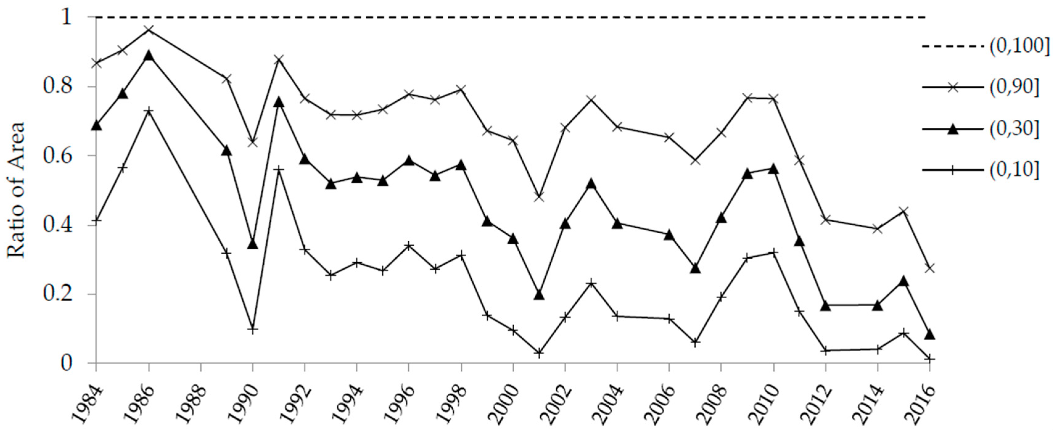
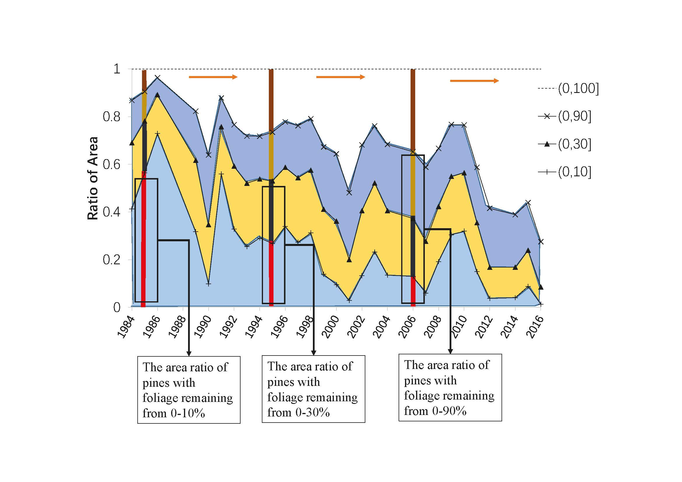
Figure 5 shows the area proportion changes of the foliage remaining ratios at different ranges by year. The area proportion was the ratio of pine area (in special foliage remaining ratio range) in the total pine area. Four foliage remaining ratio (%) ranges of (0,10], (0,30], (0,90], (0,100] were analyzed.
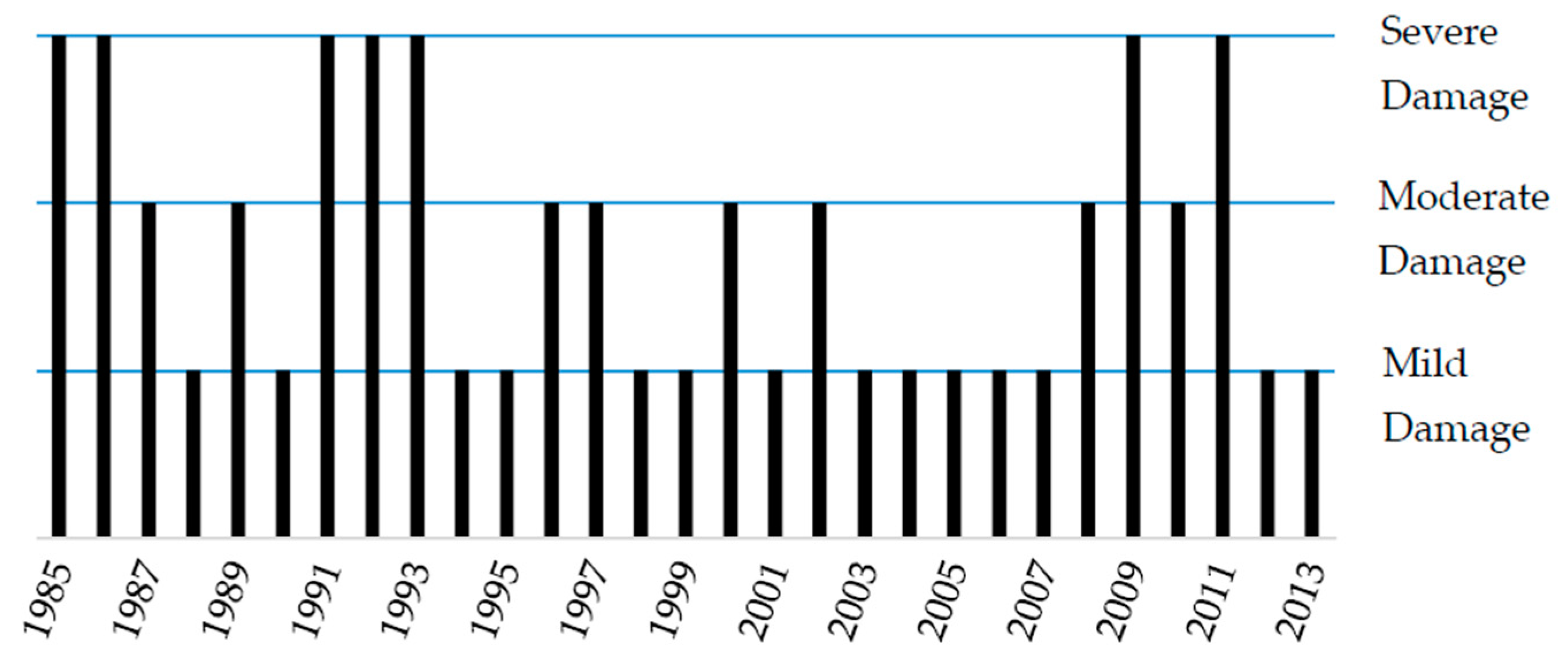
Figure 6 shows the historical degrees of damage by the pine caterpillar in the study area supplied by the local forest protection station. Comparing
Figure 5 and
Figure 6, it was found that severely damaged years (e.g., 1985, 1986, 1991, 2009) owned low foliage remaining ratios of pine forest (the proportions of (0,10) were big), and in contrast, lightly damaged years (e.g., 1990, 2001, 2007, 2012) owned high foliage remaining ratios of pine forest (the proportions of (0,10) were small). The comparison proved the reliability of the inversion results.
Compared with the traditional forest pest investigation which only divided the light, medium, and severe into three grades, the inversion method by remote sensing could supply quantitative results to assess the damage more accurately. Furthermore, the inversion results included the location of the damage, which could save a lot of costs in field investigation and supply the basis for forest workers.
3.2. Prediction in Temporal Scale
First, the best variables of the three meteorological factors needed to be determined. The correlation coefficients between the candidate meteorological variables and average foliage remaining ratios of 28 years are shown in
Table 2.
For the sunshine duration and rainfall, the best variables to select should have the strongest relevance (biggest correlation coefficients) with the foliage remaining ratios. Therefore, the annual duration (August–October and next April–July) and the rainfall of the last October were the two best variables. For the temperature, only one candidate variable was considered and its correlation coefficient was 0.512, which was sufficiently strong. Therefore, the active accumulated temperature in one life cycle was the third variable.
The average foliage remaining ratios of 28 years were regressed with the three variables and the form of regression function was:
where the Foliage Remaining is the average foliage remaining ratio; the Temp is the active accumulated temperature; the Rain is the rainfall of the last October; and the Sun is the annual sunshine duration (last August–last October and April–July).
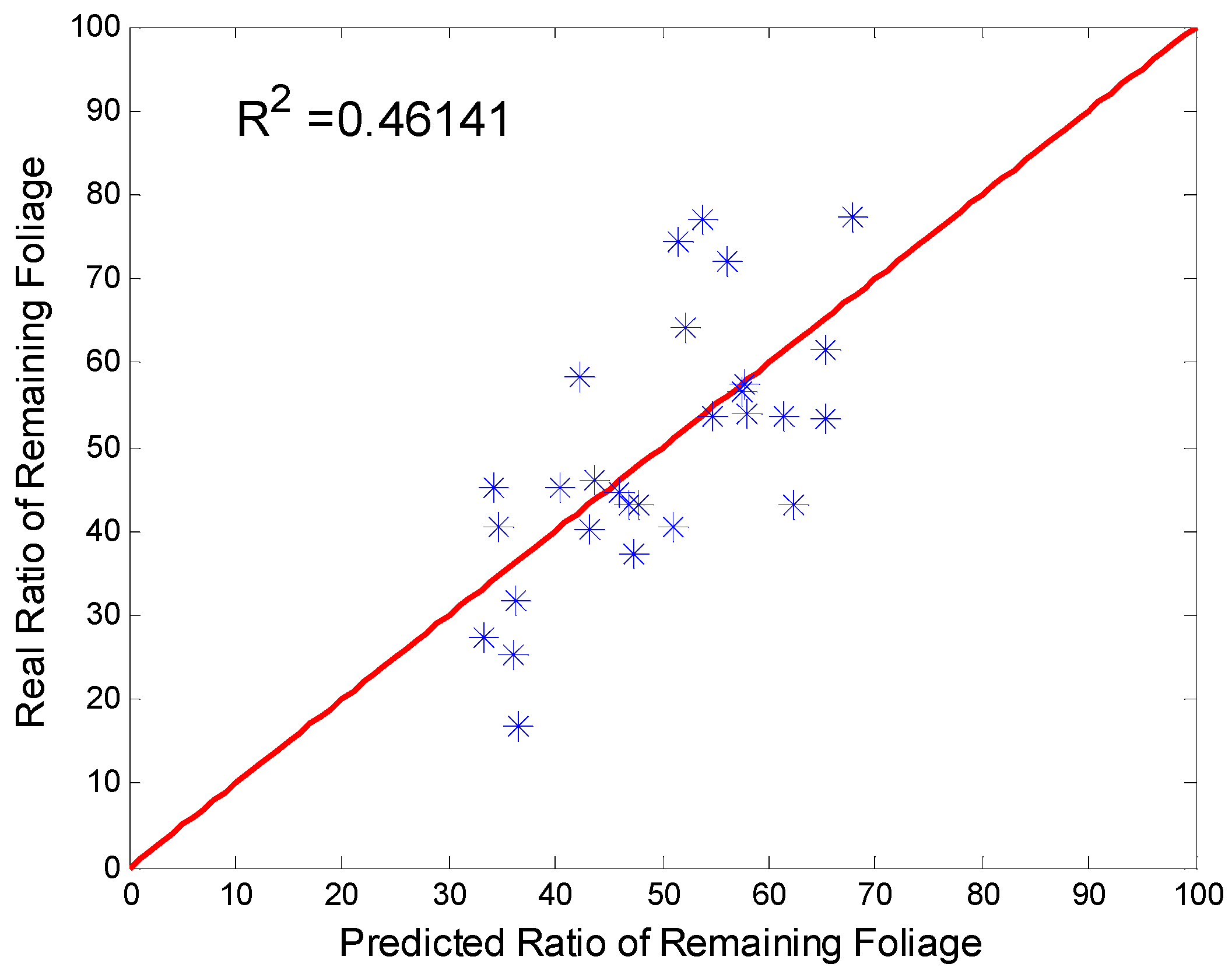
The determination coefficient of this linear function (R
2) was 0.4614. The scatter diagram of the predicted ratios and true ratios are shown in
Figure 7. The red line represents the standard line of 1:1.
Of the three kinds of meteorological factors, the temperature most strongly affected the occurrence of pine caterpillart, the rainfall affected it less, and the sunshine duration affected the caterpillar least. According to Equation (3), the increase in active accumulated temperature, the increase in rainfall, or the decrease in sunshine duration would raise the average foliage remaining ratio of pine trees in the study area. It also proved three results:
High active accumulated temperature is good at suppressing the occurrence of the caterpillar and is good for the recovery of trees.
Heavy rainfall is also good at suppressing the plague, especially rainfall in October.
Long sunshine can promote plague and activate the insect. These conformed to the biological characteristics of the caterpillar and proved the reliability of the prediction model.
The results were in agreement with our previous research [
41]. However, the determination coefficient (R
2 = 0.4614) was not so large. In general, despite the model for prediction in a temporal scale not being accurate, it still had some reference meaning for predicting the plague occurrence. The model could predict the severity of the plague in the study area preliminarily on the basis of the meteorological condition.
3.3. Prediction in Spatiotemporal Scale
The degree of damage to thepine forest is usually represented by the foliage loss ratio (or foliage remaining ratio) directly. However, in this part, the VI NDII5 was selected to indicate the severity of the caterpillar and construct the prediction model instead of the foliage remaining ratio. According to Equation (2), when the NDII5 increased, the foliage remaining ratio increased and the pine forest was healthier. Though the equation was not linear, it proved feasible to use NDII5 to represent the degree of damage to the pine trees by the following results.
3.3.1. The Best Meteorological Factors
Data across 28 years were also analyzed as the 2016 weather data was not available at the time of writing. The correlations between the candidate meteorological variables and NDII5 of random points are shown in
Table 3. A total of 5015 points were used as samples to analyze for each year, so in total, 140,420 (= 5015 × 28) sample points were counted.
According to the correlation coefficients of the three meteorological factors and NDII5, the best three variables were selected. These were the average active accumulated temperature of five years, the average sunshine duration (before and after the hibernation) of five years, and the average October rainfall of five years. The biggest correlation coefficient in temperature kind was 0.299, which meant higher active accumulated temperature would make the pine healthier and the plague lighter. The best correlation coefficient in the sunshine was −0.3729, which meant longer sunshine would make the caterpillar more active with more serious damage. The biggest correlation coefficient in rainfall kind was 0.5239, which meant that big rainfall could restrain the activity of the caterpillar and was good for pine health. These three results were in accordance with the results in the temporal prediction and the biological characteristics of the caterpillar.
3.3.2. The Transformation of Slope and Aspect
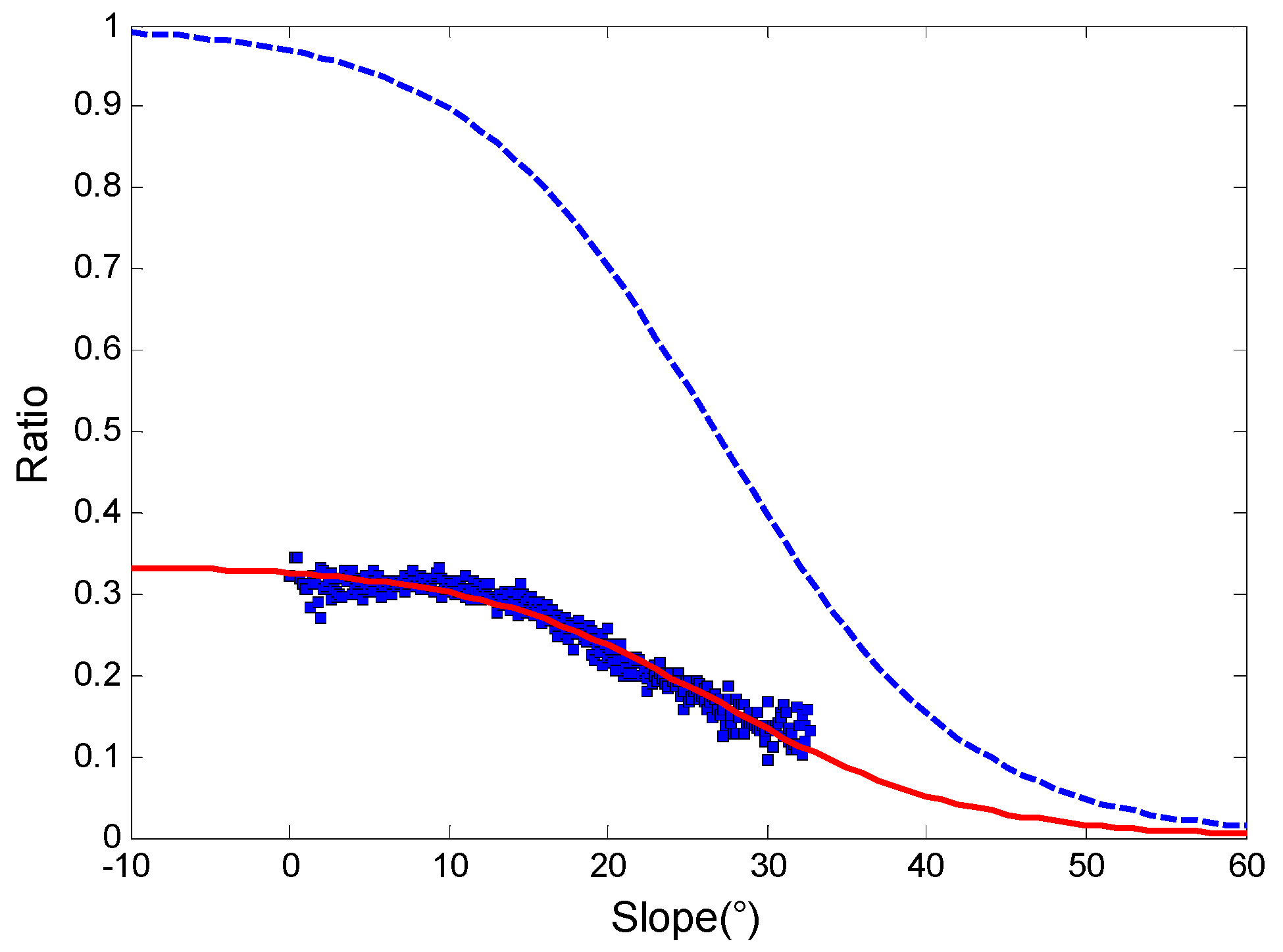
According to previous research [
41], the effect of the slope to the caterpillar was unified and the quantification relation is shown in
Figure 8. Every point on it was the area ratio of severely damaged pine forest (RVI < 4, with more caterpillars) to all pine forests in a specific slope value in 2000. Based on
Section 3.1 in this paper, RVI was feasible to distinguish severely damaged pines. Furthermore, a condition of RVI less than 4 was proved fitted in the previous research. Therefore, a threshold of RVI less than 4 was used to divide out the damaged pine. It is obvious in
Figure 8 that the ratio of damaged pine decreased as the slope increased.
A logistic function was applied to regress the points as the solid red line in
Figure 8. Its determination coefficient (R
2) was 0.9528, and the equation was:
The function could be normalized to the range 0 to 1 and obtained the dashed blue line in
Figure 8. Its equation was:
where the T_Slope is the transformed slope value, as the influence strength of slope to the pine caterpillar; and the Slope is the slope value of every pine pixel. The pine forest in the place with the biggest T_Slope was easier to damage by the caterpillar.
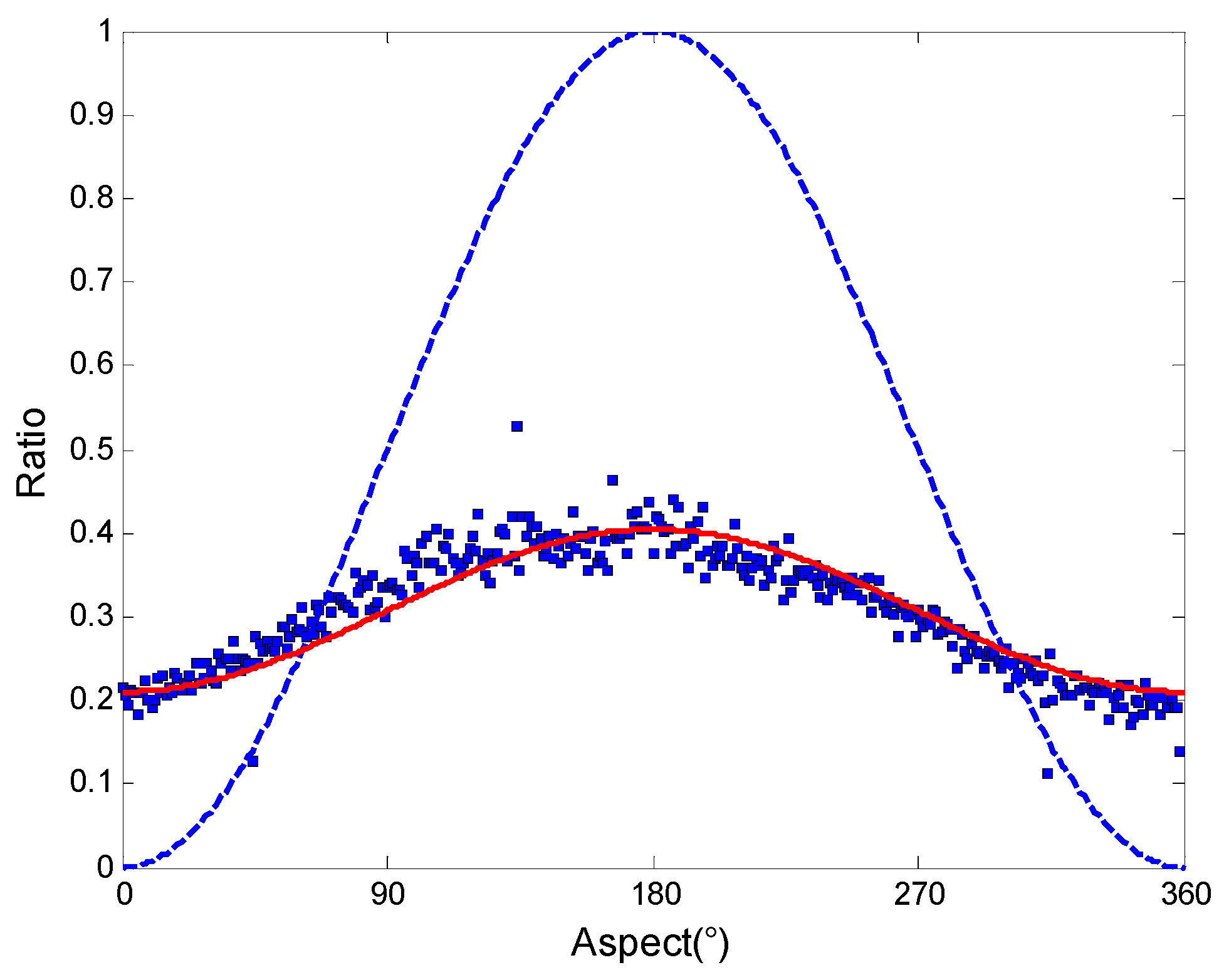
Similarly, according to previous research [
41], the effect of slope aspect to the caterpillar was unified and the quantification relation is shown in
Figure 9. Every point on it was the area ratio of severely damaged pine trees (with RVI < 4) in a specific aspect value to all pine trees in the same aspect value in the middle damaged year (2000). It was obvious from
Figure 9 that the ratio of damaged pine decreased as the aspect changed from south (
) to north (
).
A logistic function was used to regress the points as per the solid red line in
Figure 9. Its determination coefficient (R
2) was 0.8562, and the equation was:
The function could be normalized to the range 0 to 1 and obtained the dashed blue line in
Figure 9, its equation was:
where the T_Aspect is the transformed aspect value, as the influence strength of aspect to the pine caterpillar; and the Aspect is the aspect value of every pine pixel. It is known that the pine forest in the place with a large T_Aspect was easier for the caterpillar to damage.
3.3.3. The Impact of the Distance with Severely Damaged Pine Forests
The pine caterpillar is limited in its migration capability. Furthermore, the pine trees close to the severely damaged pine forests are easier for the caterpillar to infect, and are more likely to be damaged in the next year. Therefore, the distance (horizontal distance) was added as a variable into the prediction model. The effect of distance to the damage of pine was not linear and was needed to transform and make the effect of distance linear.
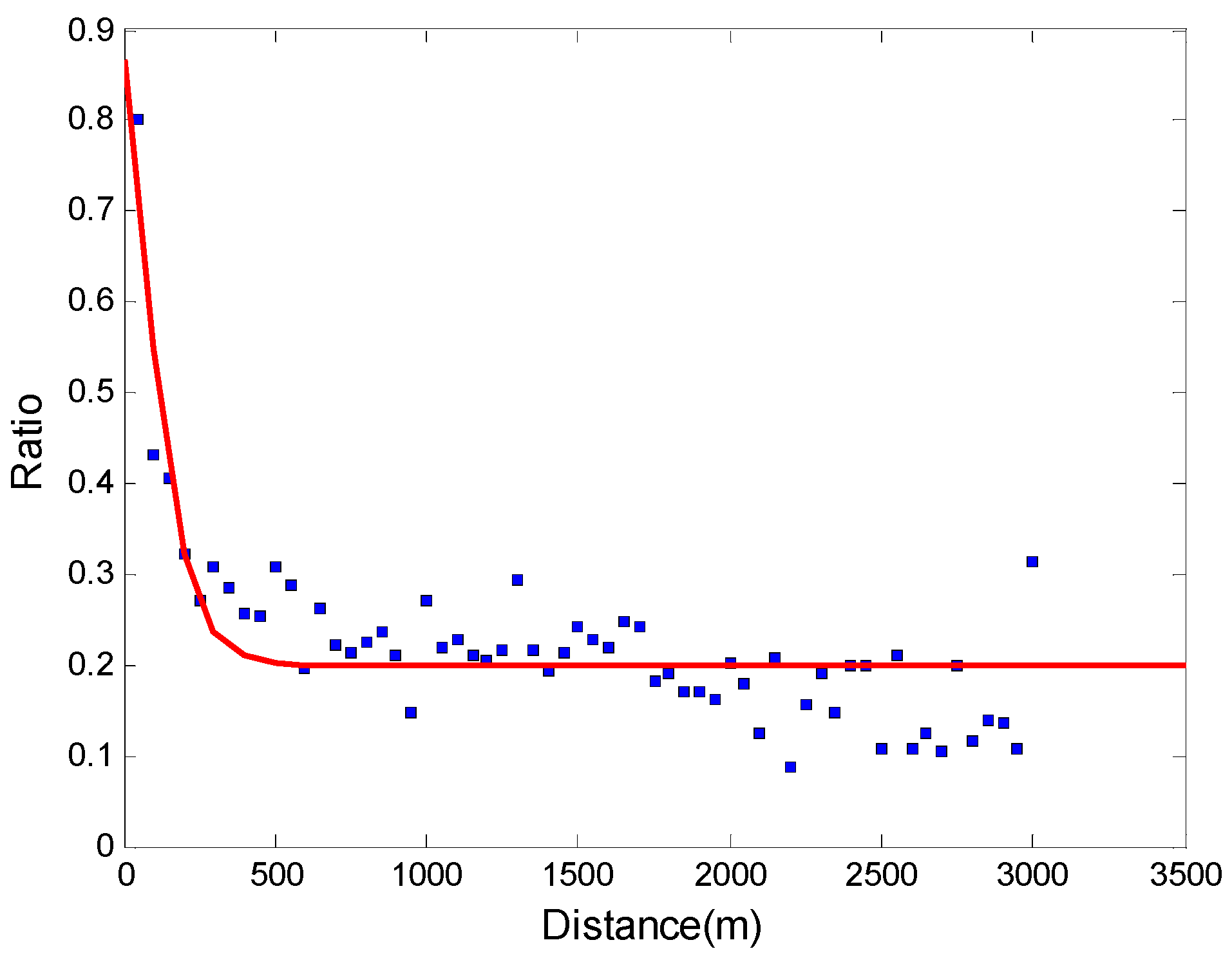
The relation of the distance and the damage was obtained as follows. The shortest distances of the 5015 sample points in five years (1985, 1999, 2000, and 2001) to the pine forests severely damaged (NDII5 < 0.1) in their last years (1984, 1998, 1999, 2000) were counted first. Then, the ratios of the points (1500 points with less NDII5 in all 5015 sample points) on the pine forests damaged relatively more seriously to all points were counted in special distance classes. Each distance class was divided with 50 m spacing. The ratios are shown in the scatter plot (
Figure 10).
From
Figure 10, the ratios tended to be steady as the distance increased, as the caterpillar only has migration ability at the moth stage and the migration distance is usually limited to a certain range. Therefore, logistic function was chosen to fit the ratios. The regression result is shown as the line in
Figure 10. Its determination coefficient (R
2) was 0.7058, and its equation was:
where the T_Distance is the influence strength of the distance to the occurrence possibility of the caterpillar; and the Distance is the horizontal distance from every pine sample point to the pine forests severely damaged in the last year.
The pine forests with larger T_Distances were easier to damage as they were near the pest source and easier to infect by the migration. According to the regression line in
Figure 10, it could be speculated that the migration limitation of the caterpillar was about 500 m in the horizontal distance as the ratio tended to the minimum when the distance was bigger than 500 m.
3.3.4. Regression Result in Spatiotemporal Model
The NDII5 values of the 5015 sample points were regressed with the least square method to construct the spatiotemporal model based on seven variables as follows:
The average annual active accumulated temperature of the last five years (Temp)
The average sunshine duration before and after the hibernation of the last five years (Sun)
The average October rainfall of the last five years (Rain)
The transformed value of the slope (T_Slope)
The transformed value of the aspect (T_Aspect)
The transformed value of the distance with the severely damaged pine last year (T_Distance)
The NDII5 value of last year (NDII5_Last).
The regression used the NDII5 of the last year as a variable. There were some disconnections in the 28 years from 1984 to 2015 as shown in
Table 1. Therefore, only 24 pairs of adjacent years could participate in the regression from all data. The sample number was 120360 (
) and the final equation was:
Its determination coefficient (R
2) was 0.6169, the correlation coefficients of the NDII5 and each independent variable are shown in
Table 4.
Considering the sample size was huge, the determination coefficient, 0.6169 was large, and the linear regression was reliable. Among the seven independent variables, the NDII5 of the last year had the strongest correlation as the migration ability of the caterpillar was weak and the recovery of the damaged pine tree was also slow. The correlation coefficient of T_Distance was negative which meant more damage happened in the pine forests near the previous year’s severe places. The correlation coefficients of T_Slope and T_Aspect were both negative and in accordance with our previous research. For the three kinds of meteorological factors, the correlation of Rain was the strongest.
In Equation (9), the coefficient of the NDII5 and Temp was negative, but its correlation with NDII5 was positive according to
Table 4. The opposite result was caused by the complex relationship between the three meteorological factors. When all three were involved into the same function, this negative coefficient of Temp was possible; however, the correlation of the NDII5 and Temp should still be positive.
3.3.5. Model Test
To test the precision of the model, every two adjacent years were inputted and tested separately. The NDII5 of the predicted year was calculated by the real NDII5 in the last year. Then, the predicted NDII5 was compared with the real NDII5 in the same year. Their correlation coefficient and error are shown in
Table 5. Furthermore, the correlation coefficient and error between the real NDII5 and the last year of NDII5 of the samples are also shown. Every statistic result was based on the 5015 sample points.
Table 5 shows that the correlation coefficient between the predicted NDII5 and the real NDII5 ranged from 0.6421–0.8725. For each year, the predicted NDII5 obtained a bigger correlation coefficient and smaller Root Mean Square Error (RMSE) than the NDII5 of the last year. This meant that the predicted NDII5 was close to the real NDII5 based on the NDII5 in the last year. The prediction ability of the model was feasible by the correction of other factors based on NDII5 in the last year.
Of the 24 predicted years, 2012 obtained the best prediction result as the error (RMSE) decreased the largest when compared to the NDII5 in the last year. There were also some years without obvious RMSE improvement such as 2002 and 2003. Their prediction results were close to the NDII5 value of the last year. The difference between the predicted NDII5 and the NDII5 in the last year was the effect of the other variables (mainly the three meteorological factors) in the model. When the effect of promoting or inhibiting the caterpillar by the other variables was not strong, the predicted NDII5 was similar to the last year’s NDII5.
To demonstrate the prediction process more clearly, the model was tested for the whole study area in the best prediction year, 2012. The result was compared with the real damage degree as an example. The raster maps of seven variables are shown in
Figure 11.
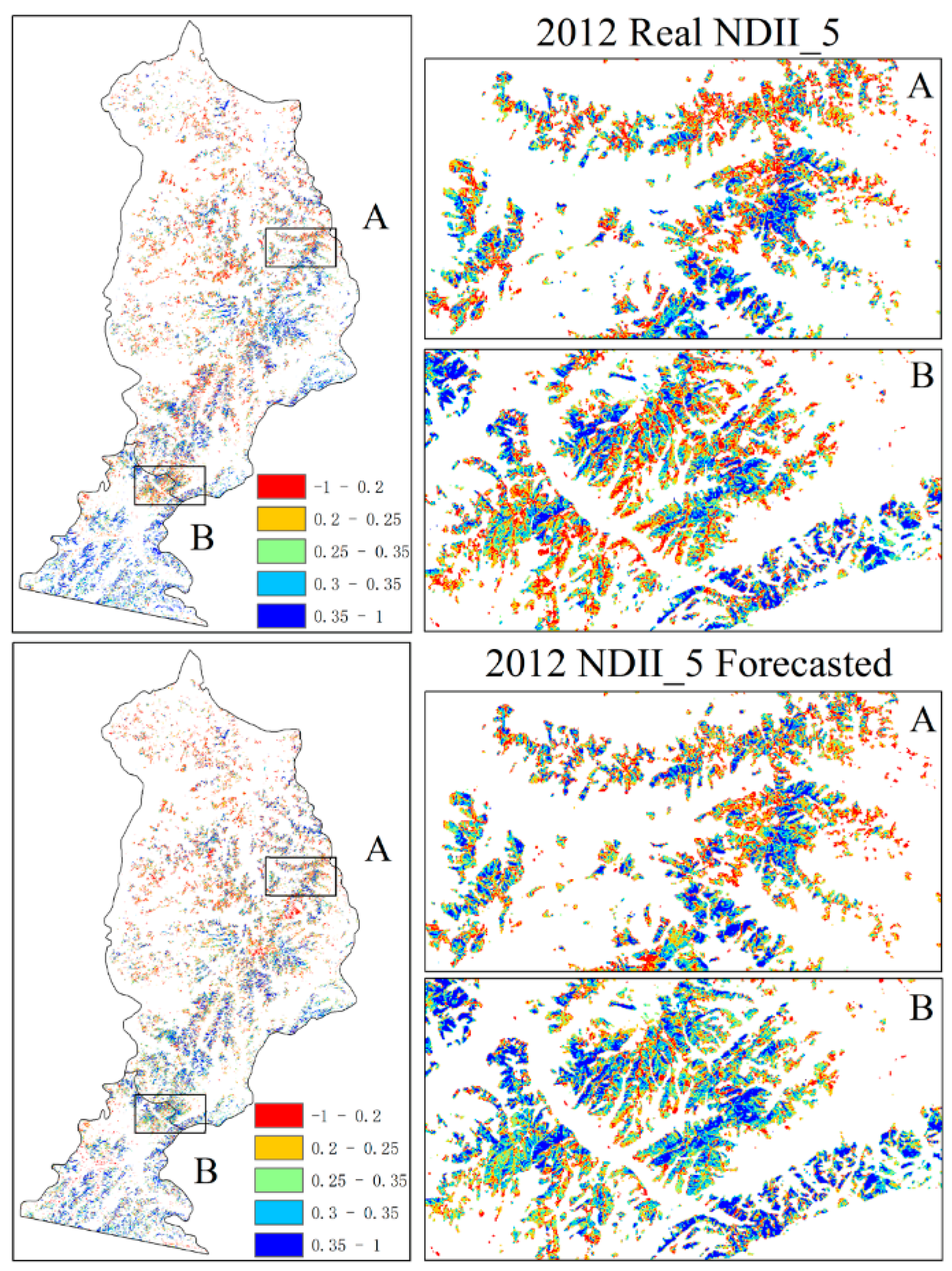
The predicted NDII5 result map and the real NDII5 map are shown in
Figure 12. The regions A and B on the map were zoomed in respectively.
Between the prediction and the reality of NDII5 in
Figure 12, the positions of relatively small and big NDII5 were consistent in general. Furthermore, the distributions of health and damaged pine trees were almost coincident. At region A, the blue area (healthy pine) in the prediction was smaller than the blue area in reality. At region B, the blue area in the prediction was bigger than the reality. However, at both A and B, the position relation between the blue (health) and the red (damaged) was the same between the prediction and the reality. This result showed that the model could effectively forecast the position of the damaged pine trees by the caterpillar, and could provide the basis for prediction of the forest pest occurrence.
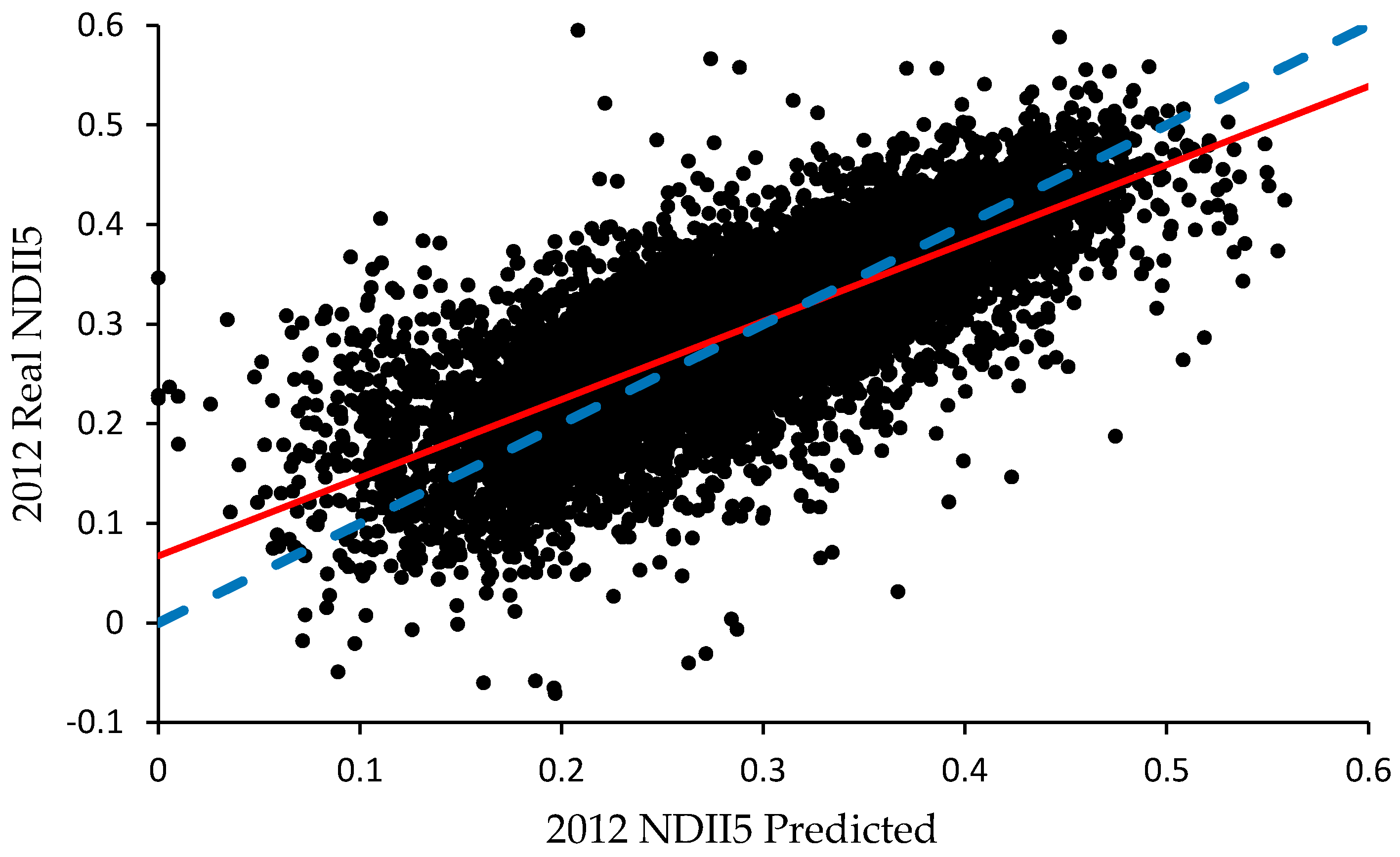
Furthermore, for validating the prediction result of the year 2012 quantitatively, another 8692 random points (with the horizontal spacing greater than 60 m) were generated at the pine forests in 2012. Their NDII5 values of the prediction were compared with the reality.
Figure 13 is the scatter plot of the compared result.
The correlation coefficient was 0.7623 between the predicted NDII5 and the real NDII5 according to the 8692 tested points. The regressed line was close to the standard line in
Figure 13. This meant that the prediction result was close to reality and the model had certain practical value.
4. Discussion
In the inversion of defoliation, NDII5 could be the optimum VI as the band involved (SWIR) was sensitive to the water content of the plant. When the pine forest was damaged by the caterpillar, its canopy lost a lot of needles. Therefore, more soil information on the image was obtained by the satellite. The needles also turned dry; as a result, the reflectance of the band (like the SWIR) sensitive to water content on the spectrum changed a lot at the pixel of damaged pine. The decrease in water content in the damaged pine was a biological reaction mechanism of self-protection for the pine tree; it could depress the larvae development and reduce further harm, given that the caterpillar larvae have poor migration. Thus, it is reliable and feasible to apply NDII5 to assess the forest damage involved with water content change.
This paper mainly took advantage of Landsat images in a long time-series and spatial public random points of pine forests. The relations of defoliation and environmental factors were obvious as the sample number used was huge. Such huge samples are difficult to obtain by traditional survey and field investigation. On the fundamental relations between the NDII5 and the seven variables, a spatiotemporal prediction model with good accuracy was obtained, which made it possible to forecast the occurrence degree and position of the caterpillar.
According to the biological characters of the caterpillar, the insect preferred dry and warm places [
40]. These were in accordance with the effects of sunshine duration and rainfall on the caterpillar, but opposite to the reaction to temperature. As the correlation coefficient of the NDII5 and the temperature showed, high active accumulated temperature caused a light plague occurrence. The reasons for this were stated as follows. In the study area, only one generation of the caterpillar occurred annually. The increase in active accumulated temperature caused the insect to grow and develop faster and led to changes in the relationships between the caterpillar and the seasons—which are natural enemies—that would break the balance of their natural relationship. Therefore, the accelerated development of the insect increased its mortality. In contrast, low active accumulated temperature caused heavy plague occurrence as lower temperatures meant the need to consume more energy for insect development, and more needles were eaten by the caterpillar to supply its growth.
There were still five deficiencies in this paper and they are stated as follows.
First, in the inversion of the foliage remaining ratio by VI, there were only 19 sample plots involved. To obtain an applicable and accurate inversion model, more field surveys and plots are needed. Furthermore, for field plots, it is better to extend the boundary length and make sure that at least one pixel of the Landsat image is in the plot completely [
27]. In this paper, the regressed result of the foliage remaining ratio by VI was distinct and acceptable. The result was not affected by the small plot boundary length (30 m) because the field plots were chosen from a big pure pine forest with a similar situation.
Second, the foliage loss for the whole study region was not only caused by the caterpillar. Other factors, like drought stress and human disturbance, could have also caused foliage loss as we investigated and brought an error to the prediction model. Especially, in mild damage years, other factors of defoliation could increase the error and reduce the inversion accuracy of the caterpillar damage. The inversion accuracy of defoliation was better in the severe damage years than in the mild damage years.
Third, the pine forests grew and the VI will change even without the caterpillar or other disturbances over thirty years [
50]. It would be better to eliminate the effect of the time change. For this aim, it is necessary to study the regular VI change of totally healthy pines at the same place over all years, and then correct the VI for each year to get rid of the influence of time. Considering the growth of the pine was relatively slow and the effect of the caterpillar was much greater than pine growth, the inversion of the defoliation ratio was still in accordance with the historical survey records.
Fourth, in the spatiotemporal prediction model, the two topographic variables in Equation (9), did not change by time. One sample point obtained the stationary value of the slope and aspect. This led to their low correlation coefficient with the NDII5. However, the topographic factors were obviously effective for the caterpillar [
41,
45]. Study is still needed on how to add the appropriate topographic variables into the model to increase its accuracy.
Fifth, in the spatiotemporal prediction model, it was good to forecast only for the next one year or few years, as the result would be worth less if forecasting too many years. Furthermore, as the data assimilation model was very suitable for long time-series prediction [
51], future study could optimize the damage prediction results by the data assimilation model. In the interpolation of meteorological factors, the interpolation result was determined by the number of ground meteorological stations, the interpolation method, and the parameters [
52]. Appropriate ground stations, methodology, and parameters could make the meteorological interpolation raster more realistic.
5. Conclusions
There were mainly three results concluded in this paper. First, the Normalized Difference Infrared Index of the 5th band (NDII5) of Landsat data, was the best VI to monitor the foliage remaining ratio and degree of damage to the pine trees. According to Equation (1), it was accessible to assess the plague of pine caterpillar efficiently and rapidly. Second, based on Equation (3), we could roughly estimate the average foliage remaining ratio of the pine and degree of occurrence of the caterpillar for the whole study region by three meteorological factors. Third, based on Equation (9), the NDII5 value could be estimated accurately at every pine forest location ( m2 region at the Landsat pixel) in the study area in any given year. Equation (9) obtained a good determination coefficient through the regression data of 120,360 samples. This meant that this model was reliable for supplying the basis for assessing the position and degree of caterpillar occurrence in advance.
In summary, the NDII5 was strongly proved appropriate for the defoliation assessment and prediction based on three lines. First, the logistic regression at the 19 plots; second, the comparison of the degree of damage to the pine in 29 years (
Figure 5) with the historical damage record (
Figure 6); and third, the relationship of the NDII5 with seven environmental factors. This relationship was in accordance with the caterpillar phenology.
These conclusions were helpful for assessing and predicting the defoliation damage done by the caterpillar and with providing forest managers with the basis to protect pine forests from plague. This prediction method could save a lot of field survey expenses for forest management.


