Vertical Deformation Monitoring of the Suspension Bridge Tower Using GNSS: A Case Study of the Forth Road Bridge in the UK

Abstract

The vertical deformation monitoring of a suspension bridge tower is of paramount importance to maintain the operational safety since nearly all forces are eventually transferred as the vertical stress on the tower. This paper analyses the components affecting the vertical deformation and attempts to reveal its deformation mechanism. Firstly, we designed a strategy for high-precision GNSS data processing aiming at facilitating deformation extraction and analysis. Then, 33 months of vertical deformation time series of the southern tower of the Forth Road Bridge (FRB) in the UK were processed, and the accurate subsidence and the parameters of seasonal signals were estimated based on a classic function model that has been widely studied to analyse GNSS coordinate time series. We found that the subsidence rate is about 4.7 mm/year, with 0.1 mm uncertainty. Meanwhile, a 15-month meteorological dataset was utilised with a thermal expansion model (TEM) to explain the effects of seasonal signals on tower deformation. The amplitude of the annual signals correlated quite well that obtained by the TEM, with the consistency reaching 98.9%, demonstrating that the thermal effect contributes significantly to the annual signals. The amplitude of daily signals displays poor consistency with the ambient temperature data. However, the phase variation tendencies between the daily signals of the vertical deformation and the ambient temperature are highly consistent after February 2016. Finally, the potential contribution of the North Atlantic Drift (NAD) to the characteristics of annual and daily signals is discussed because of the special geographical location of the FRB. Meanwhile, this paper emphasizes the importance of collecting more detailed meteorological and other loading data for the investigation of the vertical deformation mechanism of the bridge towers over time with the support of GNSS.

1. Introduction

Suspension bridges are widely utilised worldwide due to their economical nature, longevity, safety and environmentally friendly properties. The forces caused by dead, traffic and environmental loading are decomposed and undertaken by the towers and cables of suspension bridges, so longer main spans and less construction costs become achievable compared with any other bridge types. However, since nearly all the forces transferred by the cables finally become vertical stresses that are sustained by the towers, any imperfection, fatigue damage or even partial failure of the towers will ultimately reduce the capacity or even shorten the longevity of the suspension bridges [1]. Meanwhile, natural and man-made hazards, such as earthquakes, ship/vehicular collisions or extreme weather conditions, can also lead to structural damage. Therefore, it is important to understand the behavior of towers and their corresponding deformation mechanism, especially the vertical deformation that consists of subsidence, periodic signals caused by different kinds of loading forces and noise, for ensuring the structural stability, safety, serviceability and sustainability of bridges [2].

With the advancement of sensor systems, measurement and communication techniques, computational technologies and big data processing and analytical theories, structure health monitoring (SHM) systems of large civil infrastructures have been widely developed in the past two decades [3]. The main task of an SHM system is to detect fatigue damages, define and update structural and early warning models, identify key parameters, and provide timely and reliable assessment to the operation and health condition of large structures. To achieve these targets, for SHM of bridges, it is of fundamental importance to accurately quantify different loading effects (environment, traffic or geo-hazard), precisely measure corresponding responses and finally understand deformation mechanism [4].

Currently, many different types of sensors have been employed for measuring different kinds of responses such as deformation, acceleration, tension, torsion, inclination, strain and stress forces [5,6,7,8,9,10]. Global Navigation Satellite System (GNSS) technology was first used for the SHM of the Humber Bridge in 1996 [6]. It could provide deformations of centimeter- or millimeter-level accuracy at sampling rates of up to 100 Hz, and has successfully demonstrated GNSS feasibility for SHM of bridges [11,12,13,14]. It should be noticed that the high-precision kinematic deformations obtained by GNSS are related to an absolute datum and can form a long-term continuous time series in the spatiotemporal domain, which seems impossible to implement through other monitoring sensors or technologies such as a survey total station, levelling of different types, displacement gauges, accelerometers or InSAR [15,16,17,18]. Meanwhile, low-cost GNSS receivers have become more popular in the SHM since they can provide nearly identical positioning performance to the high-end geodetic receivers [19,20]. Thus, denser monitoring network can be deployed to support the more detailed health condition analysis and assessment of the large infrastructures. Due to these unique characteristics, GNSS can provide an opportunity to understand the behavior and deformation mechanism of the suspension bridge tower based on the long-term deformation time series, which has not yet been properly studied so far.

This paper focuses on the vertical deformation monitoring and its mechanism explanation of the bridge tower since most of the forces on the tower is vertically downwards and its stability along the axis direction of the bridge is maintained by the main cables. The deformation and stability on lateral direction, which is perpendicular to the plane governed by the vertical and bridge major axis directions, are mainly affected by the wind-induced loadings [21], but we do not discuss this topic in this paper. As mentioned above, the vertical deformation of the towers consists of different components caused by different kinds of loading, of which the effects should be separated for the mechanism explanation. To attain this goal, a case study of the FRB is carried out in this paper.

Firstly, a data processing strategy is designed that covers each step from data acquisition to the final analysis. Then, the real vertical deformation time series of the bridge tower with 33 months of data provided by GNSS is used for the first time, and a classical function model with noise signals for the GNSS coordinate time series analysis is adopted to isolate the linear subsidence and other periodic signals [22,23]. Finally, a subsidence rate of 4.7 mm/year is achieved with 0.1mm standard deviation (STD). The annual and daily signals with their relevant harmonics are obtained with spectral analysis. Since the thermal expansion causes the seasonal signals in the GNSS short baseline coordinate time series, a classical linear expansion model with relevant coefficients is used and demonstrated in this paper. With the support of 15-month meteorological data, the vertical deformation time series simulated by the thermal expansion model is compared with the actual GNSS vertical deformation time series. The annual amplitudes correlate well between these two time series. However, the phase of these two time series does not correlate well, and significant differences exist during particular periods. The analysis of daily signal is also carried out with the utilisation of ambient temperature data. Finally, the potential contribution of the North Atlantic Drift (NAD) to the inconsistent characteristic of both annual and daily signals is discussed.

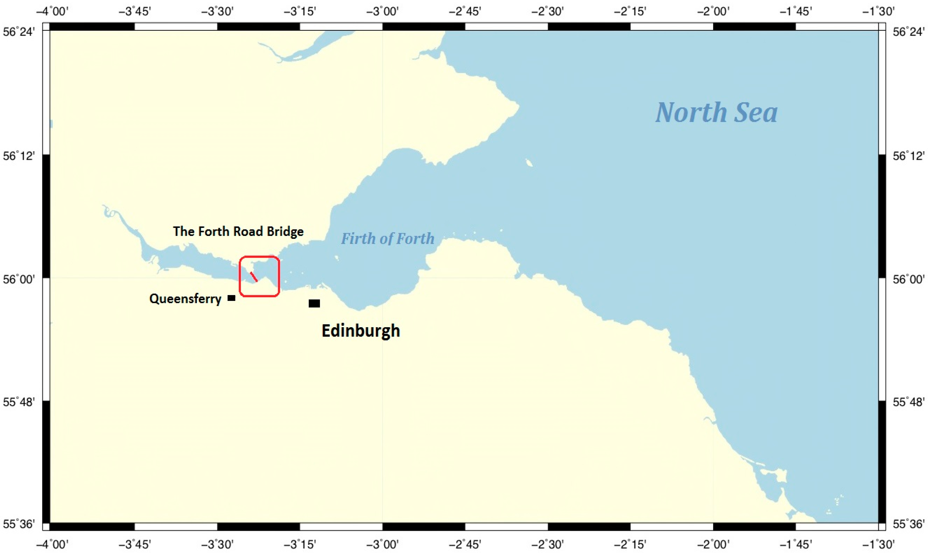
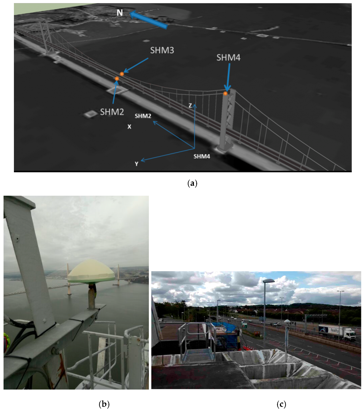
2. The Forth Road Bridge and Its Monitoring System, GeoSHM

The FRB is located on the west coast of the North Sea and the Firth of Forth gulf, as shown in Figure 1. It is a long suspension bridge with a main span of 1006 m between its two bridge towers. It began to operate in 1964 as the main road transportation hub between the north of Scotland and the south, and it was the largest bridge in the world outside the United States with a total length of 2512 m when it was constructed. The two main towers reach about 150 m above mean sea level (MSL), with welded cellular high tensile steel construction. The detailed structures of the FRB are introduced in [24]. According to the data record collected in 2009, the traffic volume of the FRB has increased by about 6-fold from 4 million in 1964 to approximately 24 million vehicles per year [25]. The traffic loading is therefore significantly higher now than its expected values that were designed in the 1960s. Also because of the transportation requirements of heavy good vehicles, the main towers have been strengthened in the late 1990s. However, since more than 20 years have passed with rapid development of economy and transportation, the structure and health of the FRB, especially the main towers, still captures the attention of engineers, stakeholders, governments and general public.

For the feasibility demonstration of using integrated GNSS positioning and Earth Observation (EO) techniques for SHM, a GeoSHM Feasibility Study (FS) project led by the University of Nottingham was launched in September 2013 and completed in September 2015 with the funding and support of the Europe Space Agency [26]. Three high-end Leica GNSS receivers were deployed on the FRB (two on the middle span and one on the west of the South Tower, as shown in Figure 2), while one GNSS receiver with the same type was set on the FRB control building on the southern shore as the reference station. For the aim of understanding the relative deformation of the FRB, a local reference datum is defined as shown in Figure 2a, the X, Y and Z directions represent the longitudinal, lateral and vertical directions, respectively. Then, a long-term vertical deformation time series with high precision can be achieved by GNSS for the comprehension of the behaviour and corresponding mechanism of the south of the FRB.

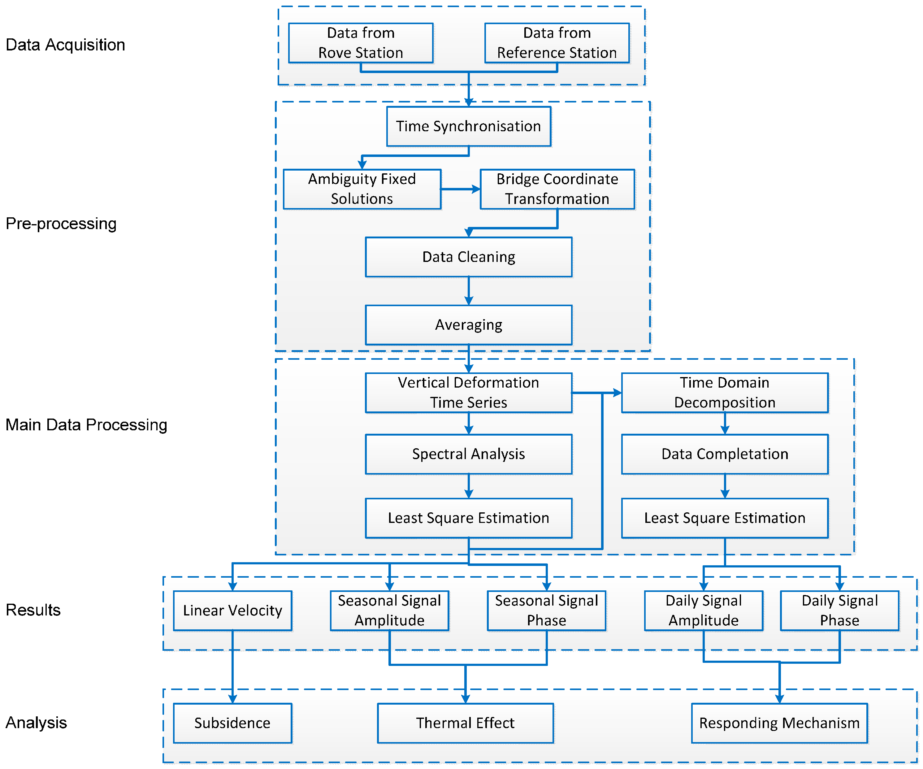
3. Data Processing Strategy

As mentioned before, a deformation time series of the South Tower site on the FRB covering 33 months from January 2015 to September 2017 is prepared. Then, a spectral analysis is carried out to understand the distribution of periodic signals and the noise characteristics. A classical function model for GNSS coordinate time series analysis is adopted here with a properly selected noise model. Finally, the detailed information of subsidence and other periodic signals are obtained. The detailed data processing strategy is exhibited in the flowchart in Figure 3.

3.1. GNSS Data Pre-Processing

In this paper, the traditional GNSS double-difference technique is adopted here with a very short baseline between stations SHM1 and SHM4. The 10 Hz GNSS raw data are processed by Leica Spider software and the resulting coordinates are transformed to the local reference datum as displayed in Figure 2a. For the discussion of this paper, only the ambiguity-fixed solutions are used for the vertical deformation time series analysis since the precision of the deformation obtained by GNSS cannot reach the centimeter or even millimeter level if the ambiguity is not correctly fixed [27,28]. Then, an averaged deformation every 10 min is used to analyze the correlation between the deformation and the loading of different types, especially the temperature and wind-induced loadings [29,30]. Another reason for the 10-min average is that 15 months of meteorological data also uses a 10-min sampling interval. In this paper, an equally weighted model is adopted for the calculation of the averaged deformation and related STD, exhibited in Equation (1):

$$\overline{x}=\frac{1}{n}{\sum }_{i=1}^n{x}_i,u_x=\sqrt{\frac{{\sum }_{i=1}^n{\left(x_i-\overline{x}\right)}^2}{n-1}},$$

(1)

where $\overline{x}$ denotes the averaged deformation, n is the number of ambiguity-fixed solutions in each relevant data block, $x_i$ denotes the deformation of epoch $i$ and $u_x$ denotes the STD of the averaged deformation $\overline{x}$. In practical data processing, three-dimensional deformation (3D) time series can be expressed with relevant STDs $\overline{x}\pm u_x$.

Since a possibly bad satellite geometry and observation environment would result in incorrect estimation of cycle slips and ambiguities, the resultant gross errors should first be removed in order to obtain a clean GNSS vertical deformation time series. In this paper, absolute tolerances of 0.15 m and 0.1 m are adopted in the first step with the relevant medians of the horizontal and vertical deformations to remove the distinct gross errors before the averaging processing shown in Figure 3. Then, $3\mathsf{\sigma }$ (the standard deviation $\mathsf{\sigma }$ is regarded as equal to the root mean square error) is used with a 99.73% confidence level to further clean the deformation time series. The final GNSS deformation time series are shown in Figure 4. It is clear that some data gaps exist in the time series. The possible reasons are that the GNSS observations may be affected by the multipath error, the ambiguity resolution is not correct, the existing GNSS constellation geometry at high-latitude regions is deficient, and the performance of the hardware might be not stable at these specific high-rate applications, which would result in a failure to achieve high-precision deformations. Also, the excessive vibration of the FRB and abnormal operation of the system would lead to some data acquisition and connectivity problems since the raw measurements are transmitted by the optical fiber to the local hub. It should be noted that the data gaps in the deformation time series would not be filled in by numerical methods in order to get real periodic signal distribution through spectral analysis.

3.2. The Processing of the Vertical Deformation Time Series

The vertical deformation time series gives insight into the relative deformation of the GNSS station located on top of the South Tower of the FRB from January 2015 to September 2017. Here, it will be used to verify the deformation behaviour, such as subsidence, periodic signals and noise, with the relevant mechanism of the tower deformation during this period.

According to Figure 4, the vertical deformation time series seemed to be stable with a STD value less than 5 cm. In addition, some seasonal signals are apparent, which can also be seen in the time series of the X direction. The crest occurs around June, while the trough occurs around January or February, which clearly demonstrates the seasonal deformation change of the South Tower. Before the estimation and analysis of the periodic signals, the spectral analysis is carried out to preliminarily understand the distribution of the periodic signals in the frequency domain. The power spectral density (PSD) values of the vertical deformation are shown in Figure 5. It can be inferred that there is an obvious oscillation around the annual period with a 365.2-day period, which is called the tropical year oscillation [31]. Besides, there are some peaks around the diurnal period (24 h) and its harmonics. For the time series analysis, the selected stochastic model can affect the estimated parameters in the functional model, especially for the STDs of the velocity and seasonal amplitudes [32,33,34]. Analysis of the coordinate time series of global IGS stations suggests that the optimal noise model is a combination of flicker and white noise instead of white noise alone [35]. However, the optimal noise model varies from site to site [23]. The spectral index of flicker noise is –1, which means the slope of PSD should be equal to −1. However, it is difficult to see this specific slope value in Figure 5. So the effect of flicker noise seems to be weak and can be neglected in this paper. Meanwhile, considering the massive amount of the time series and huge computation burden (more than 130,000 epochs), the stochastic process is assumed to be white noise in this paper.

To quantitatively analyze the coordinate time series variations, we simultaneously compute the velocity, the amplitudes and phases of the seasonal signals. Then, a function model that is widely used in analysis of GNSS coordinate time series is adopted [22,36,37,38]. The model contains a linear velocity, an offset, harmonics of the tropical year oscillation and noise. The velocity refers to the linear trend during the time span, which can reflect the subsidence of the bridge tower:

$$Z=velocity·t+offset+{\sum }_{i=1}^n{A}_{i}sin\left({\omega }_i·t+{\phi }_i\right)+\epsilon ,$$

(2)

where $A_i$, ${\omega }_i$ and ${\phi }_i$ are the amplitude, the angular frequency, and the phase of each annual harmonic i, respectively. The number of the harmonic n is chosen to be 2, which refers to the annual and semi-annual oscillations.

4. Results

The least-squares estimation (LSE) is used here to acquire the value of each parameter based on the white noise stochastic process assumption [39]. The estimated parameters are listed in

Table 1. The estimated linear velocities, seasonal amplitudes, and relevant phases.

Component	Linear Velocity (mm/year)	Annual Oscillation		Semi-Annual Oscillation
		Amplitude (mm)	Phase (°)	Amplitude (mm)	Phase (°)
Z	–4.7 ± 0.1	9.3 ± 0.1	239 ± 1	0.7 ± 0.1	277 ± 8

. The results show that the linear trends of −4.7 mm/year are observed on the Z components, which indicates that the GNSS station located on the top of the South Tower experiences a gradual subsidence with a rate of about 4.7 mm/year. At the same time, an annual oscillation with 9.3 mm amplitude is also achieved, as shown in Figure 6, where the linear trend has been excluded.

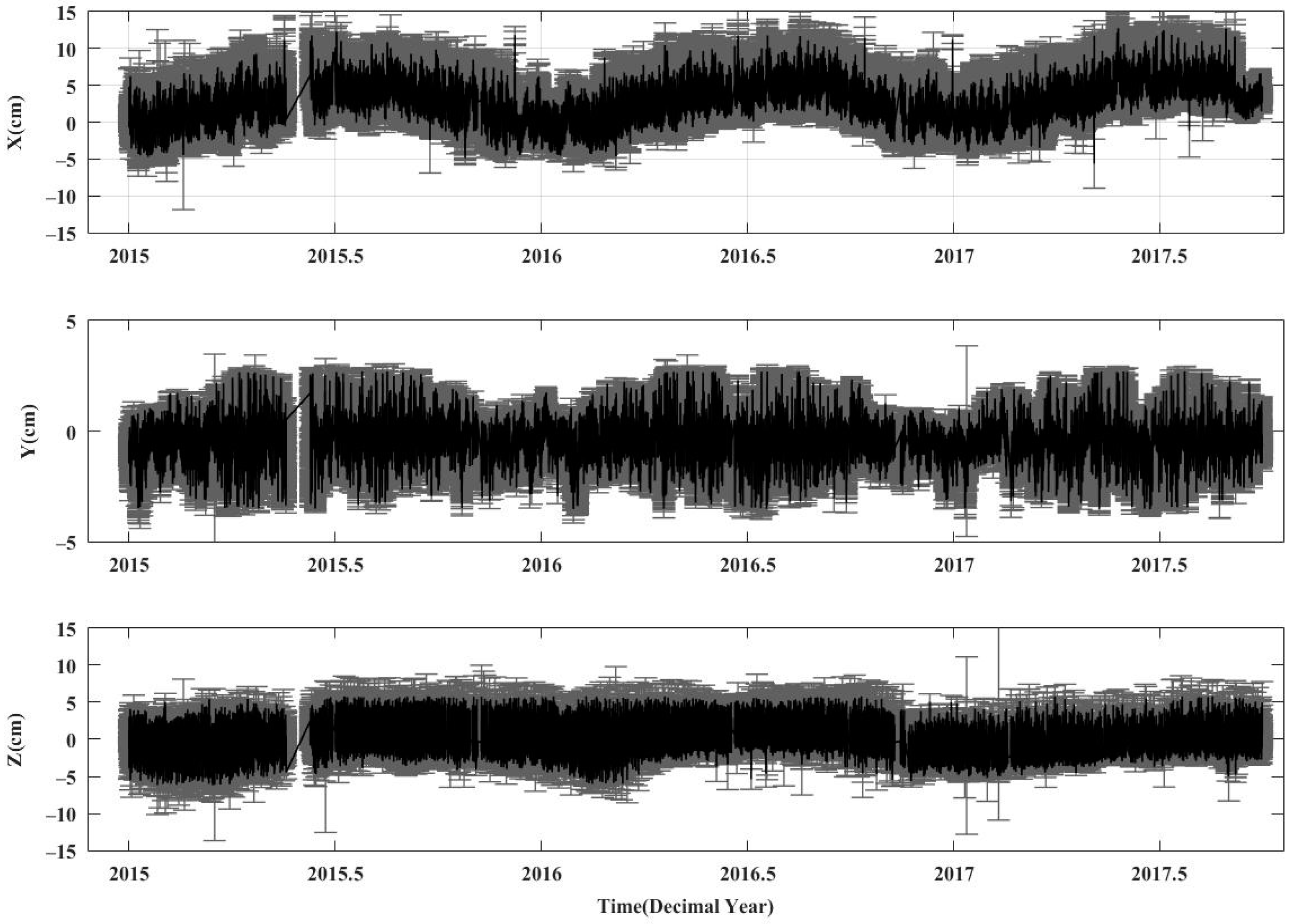
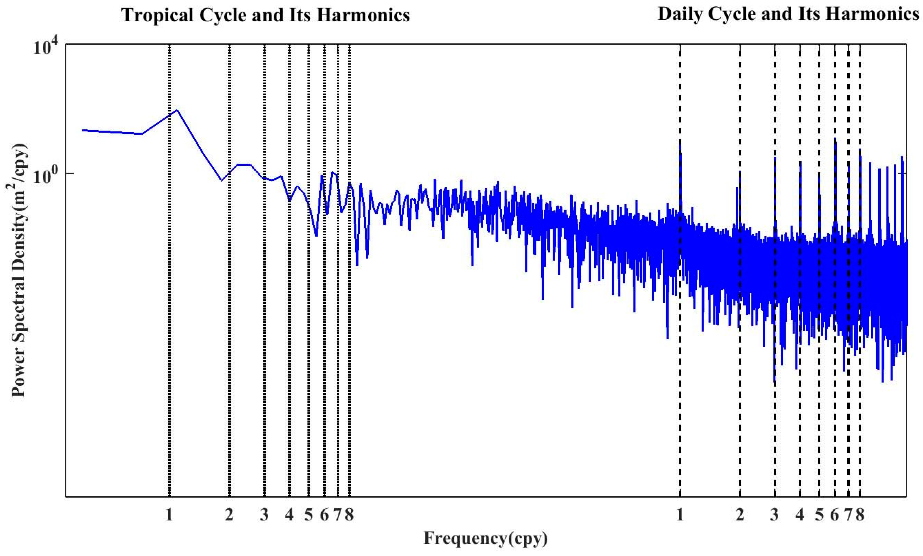
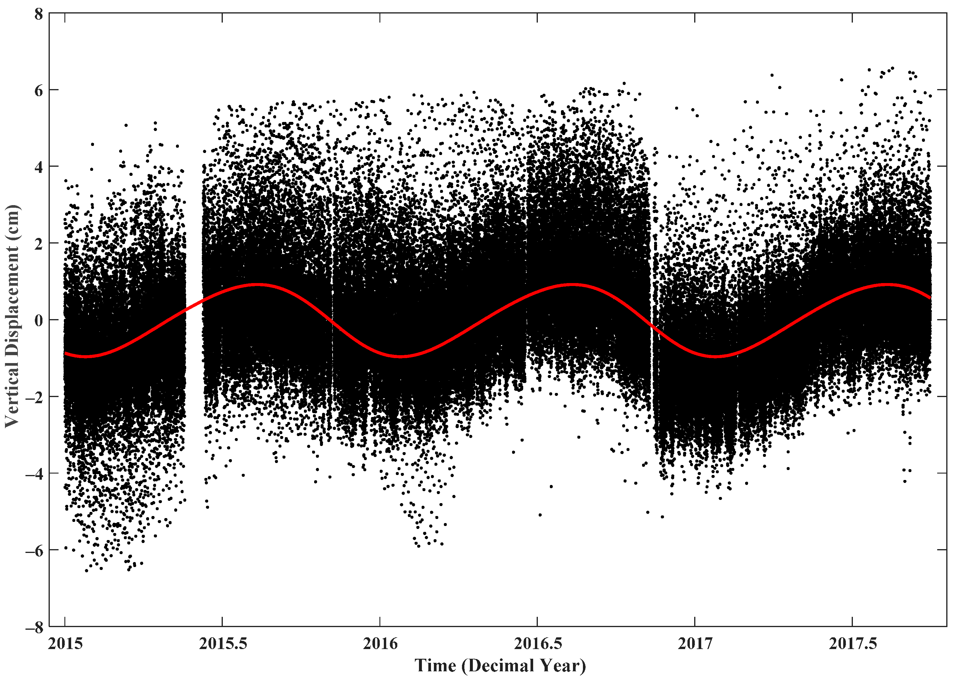
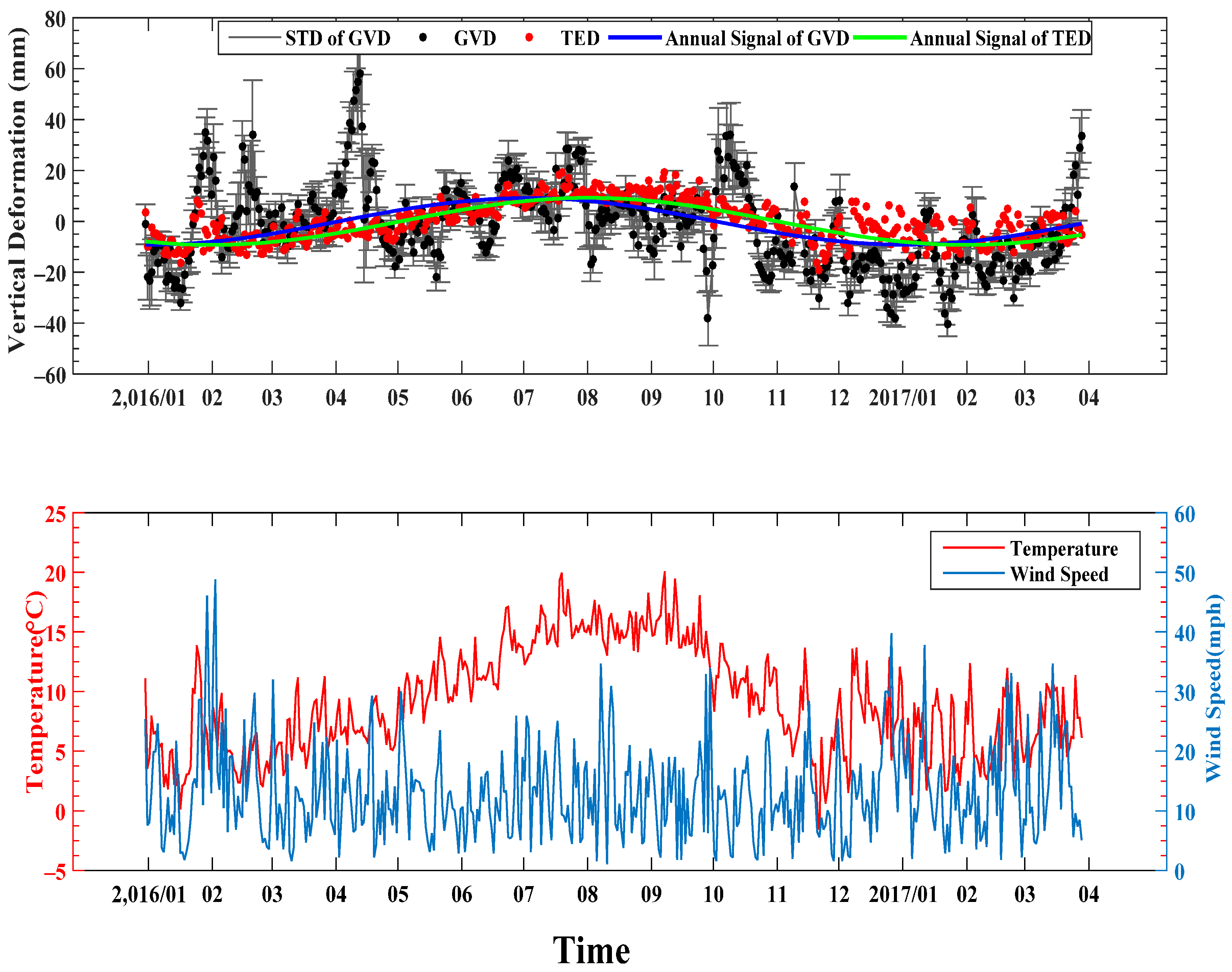
4.1. Annual Signal Analysis

For analysing the possible factors that can introduce periodic signals in the vertical deformation time series, the effect of horizontal deformation is discussed. From Figure 4, it is evident that the deformation fluctuations in the X and Y directions are smaller than 0.2 m and 0.1 m, respectively. Here, the value of horizontal deformation s is set to be 0.3 m, which is larger than its actual values. The height of the tower h is set to be 150 m according to the discussion in Section 2. Then, we can compute the vertical deformation caused by the horizontal deformation according to the procedures in Figure 7. The approximate value of the resulting vertical deformation $\Delta \mathrm{h}$ can be obtained as 0.06 mm, which is substantially smaller than its actual value displayed in Figure 4. Therefore, it can be demonstrated that the horizontal deformation would make nearly no influence on the change of the vertical deformation. The wind-induced loading mainly affects the horizontal deformation of the bridge towers, especially in the Y direction of Figure 2a, which is difficult to stabilize with cables [40]. So, the effect of wind-induced loading is also excluded.

Thermal effects induced by the solar radiation and ambient temperature would lead to the expansion or contraction of different components of bridges, especially the cable-supported bridges, and result in daily, seasonal, and annual signals [41]. Currently, apparent periodic signals are also observed in GNSS coordinate time series in previous research [42], including the annual and semi-annual patterns. Similar seasonal signals are also captured in the coordinate time series by using GNSS short-baseline positioning since most GNSS observations and systematic errors are diminished or even eliminated [36,43]. Besides, these seasonal signals are more significant, while the station pair has large height differences between their observation monuments (the monument is defined as the structure that attaches the antenna to the surface of earth) [44]. Finally, it has been demonstrated that the local effects such as thermal expansion are dominated in the GNSS coordinate time series [36].

For the monitoring of SHM4, the traditional DD technology with a short baseline (less than 2 km) is applied, and most of GNSS inherent errors and seasonal signals induced by large-scale geophysical phenomenon such as plate movement are substantially mitigated. The bridge tower, in some sense, can be regarded as an observation monument with super large-size, so the contribution of thermal effect to the seasonal signals of the vertical deformation time series of the tower is discussed [42]. In order to estimate the vertical deformation induced by thermal expansion, a classical linear expansion model is introduced in Equation (3):

$$D_{TE}=\alpha ·L·\left(T-\overline{T}\right),$$

(3)

where $D_{TE}$ denotes the vertical deformations, $\alpha$ denotes the linear expansion coefficient, L denotes the length of the monument beneath the GNSS antenna, T and $\overline{T}$ denote the observed surface temperature and average temperature of monument, respectively. For the bridge tower in this paper, the linear expansion coefficient of steel structure $\alpha$ is set to be $1.2\times {10}^{-5}/°\text{C}$, which has been demonstrated in the research of thermal actions of civil infrastructure [45] and GNSS coordinate time series [42], and the length of the tower is set to be 150 m above the mean sea level. It should be noted that the thermal expansion coefficient varies with the temperature, but it can be treated as a constant over small temperature ranges [46]. As shown in Figure 8, the maximum fluctuation of air temperature is less than $30$ °C in 15 months. Although the structural temperature of the tower is not equal to the air temperature, the variation of thermal expansion coefficient is not considered in this paper.

The temperature data, particularly the structure temperature of the tower, are essential to the analysis of its thermal expansion effect. Unfortunately, there are no structure temperature data available and thus the air temperature data collected from January 2016 to March 2017 with a temporal resolution of 10 min are used instead. The duration of the temperature data is more than a year, which allows the estimation of annual signals. For better comprehension of the thermal effects and to mitigate the impact of high-frequency signals on the time series, we sub-sample both the GNSS vertical deformation time series and the observed temperature and wind speed time series to daily solutions. The epoch at 12:00:00 of every single day is chosen for the sub-sampling processing. The GNSS vertical deformation (GVD) and the modelled thermal expansion deformation (TED) time series are both shown in Figure 8.

Table 2. The estimated seasonal amplitudes and phases of the GVD and TED time series.

Component	Annual Oscillation		Semi-Annual Oscillation
	Amplitude (mm)	Phase (°)	Amplitude (mm)	Phase (°)
GVD	9.2 ± 1.8	268 ± 12	5.6 ± 1.8	293 ± 18
TED	9.3 ± 0.6	240 ± 4	2.1 ± 0.6	11 ± 16

lists the estimated seasonal amplitudes and phases of the two time series.

Finally, the estimated annual amplitudes and phases of GVD are 9.2 ± 1.8 mm and 268 ± 12 degrees, respectively, which is consistent with those of TED of 9.3 ± 0.6 mm and 240 ± 4 degrees with the configured linear expansion coefficient. The consistency reaches 98.9%. However, the fluctuations of GVD and TED in Figure 8 do not correlate well, especially during the period close to the end of every year, such as those from January 2016 to April 2016 and from October 2016 to April 2017. However, this inconsistent characteristic becomes less significant from May 2016 to September 2016. The STDs of GVD in Table 2 are significantly larger than those in Table 1. The main reason is that there are more redundant observation while the 10-min averaged vertical deformation are used, which can improve the performance of LSE.

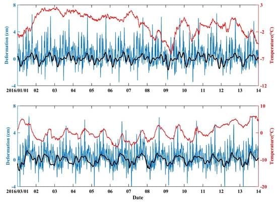
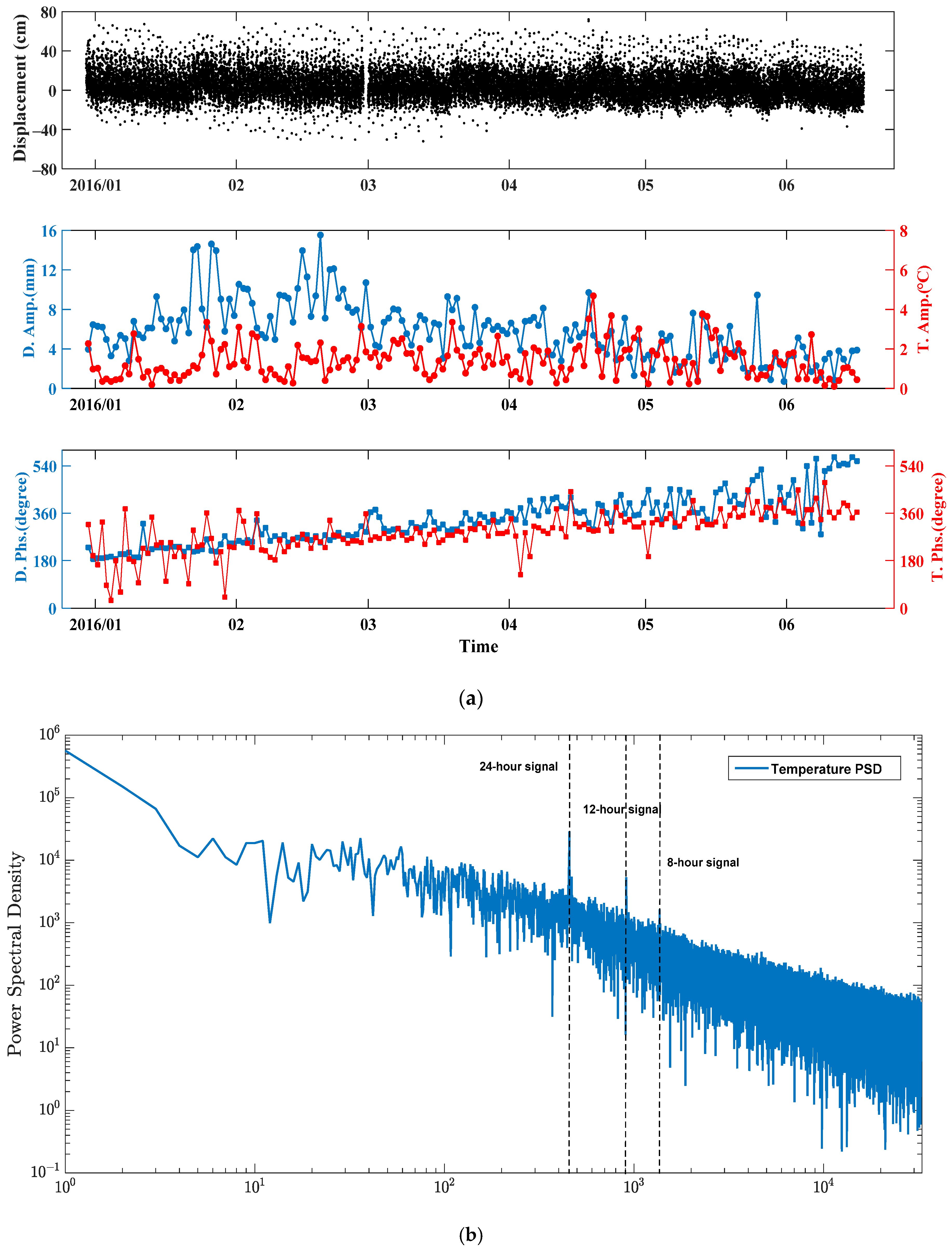
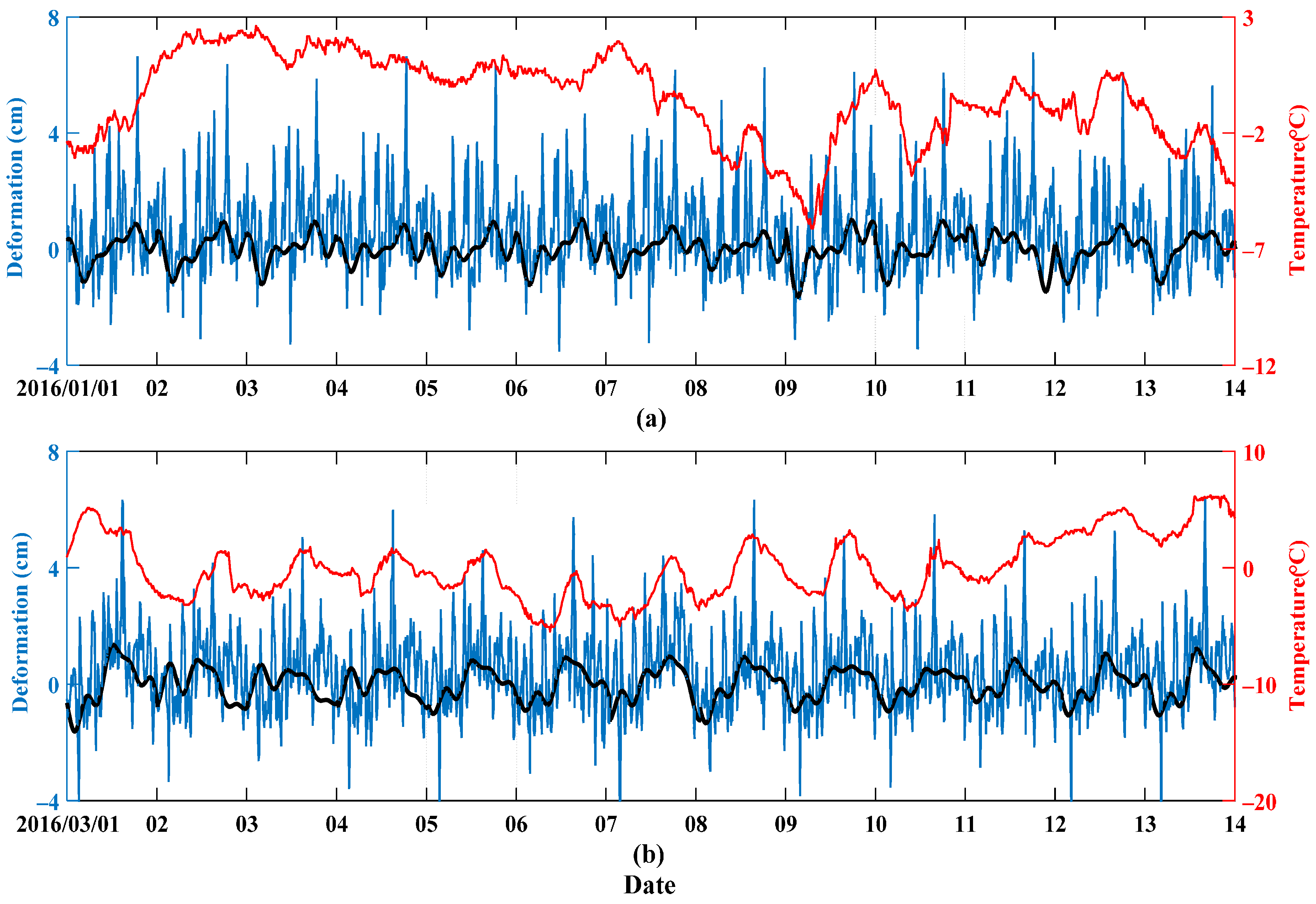
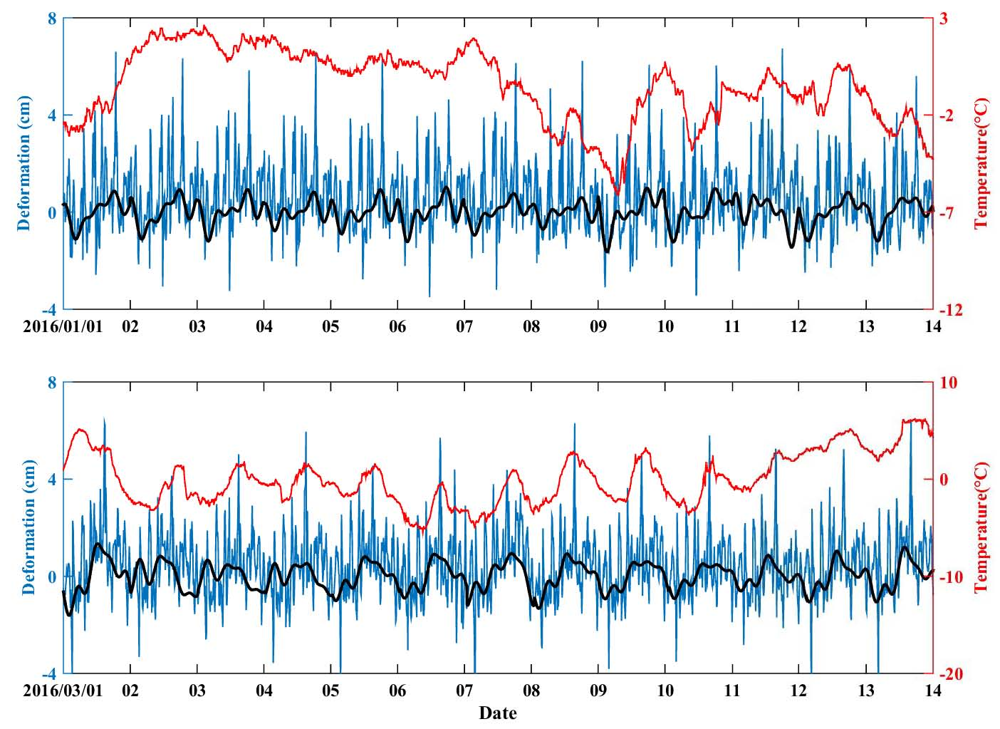
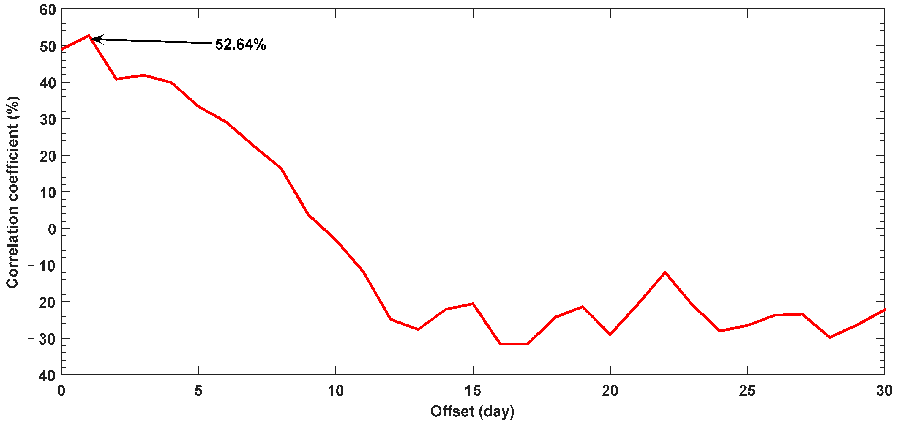
4.2. Daily Signal Analysis

For the analysis of daily signal and its harmonics, the 10-min averaged vertical deformation time series from 30 December 2015 to 16 June 2016, with a length of 170 days, is adopted because of its high data integrity and the existence of relevant meteorological data. Since only 24 epochs are missing (total number of epochs: 24,480), all the missing epochs are filled in by cubic spline interpolation. The linear trend, annual signal, and its harmonics are removed through time domain composition, as shown in Equation (4):

$$Z_{new}=Z_{raw}-velocity·t-offset-{{\displaystyle \sum }}_{i=1}^2{A}_{i}sin\left({\omega }_i·t+{\phi }_i\right),$$

(4)

where $Z_{raw}$ denotes the raw 10-min averaged vertical deformation time series; $Z_{new}$ denotes the resulting vertical deformation time series that excluded the effect of linear trend, annual signal and its harmonics. The resulting vertical deformation time series is displayed in Figure 9a.

As shown in Figure 9b, the PSD values of air temperature data clearly display the oscillation around the daily period with 24 h and relevant 12-h or eight-hour period harmonics. Here, the LSE is utilised for the parameter determination of daily signal and its harmonics, include amplitude and phase. For this purpose, the eighth harmonics with a one-hour period are considered and the higher harmonics can be neglected, as displayed in Equation (5) [31]:

$$\begin{array}{c}{Z}_{raw}={\displaystyle \sum }_{j=1}^8{A}_{j}sin\left({\omega }_j·t+{\phi }_j\right)+{\epsilon }_z\\ T={{\displaystyle \sum }}_{k=1}^3{A}_{k}sin\left({\omega }_k·t+{\phi }_k\right)+{\epsilon }_T,\end{array}$$

(5)

where A, $\omega$ and $\phi$ are the amplitude, the angular frequency and the phase of each harmonic, respectively. j and k represent the jth and kth harmonics of vertical deformation $Z_{raw}$ and temperature T, respectively.

The amplitude and phase results of the daily signal of the vertical deformation and temperature data are shown in Figure 9a. It seems that the amplitude results of vertical deformation and ambient temperature do not correlate well. The major reason is that the temperature data collected by the meteorological instrument deployed on the deck of the FRB cannot reflect the actual condition of the structural temperature of the tower in a short period of time considering the complicated meteorological change and the high structural construction of the tower. However, the variation trend of the phase results becomes highly consistent from February 2016. Here, two specific periods of time are selected: 1 January 2016 to 14 January 2016 and 1 March 2016 to 14 March 2016. It can be seen from Figure 9a that the phase fluctuation of the temperature data from 1 January 2016 to 14 January 2016 is sharp; the major reason is there is nearly no daily signal inside the temperature data, as shown in Figure 10a. At the same time, the phase results of vertical deformation and temperature data have good consistency and stable variation tendency from 1 March 2016 to 14 March 2016 as shown in Figure 10b; this identifies the correlation between the vertical deformation and the ambient temperature. However, since there are no other data available, such as traffic or meteorological data, including steel structure temperature, wind speed, etc., it is still unclear what the detailed mechanism is of the daily signal inside the vertical deformation. The fitting vertical deformation time series with the parameters achieved by the LSE of Equation (5) correlate quite well with the real vertical deformation time series, as displayed in Figure 10. This demonstrates the good performance of the LSE. However, there are significant differences of several centimeters between these two vertical deformation time series. A possible reason is that the positioning performance of GNSS have been affected and the repeated peaks reflect that some systematic errors may exist, which needs further research.

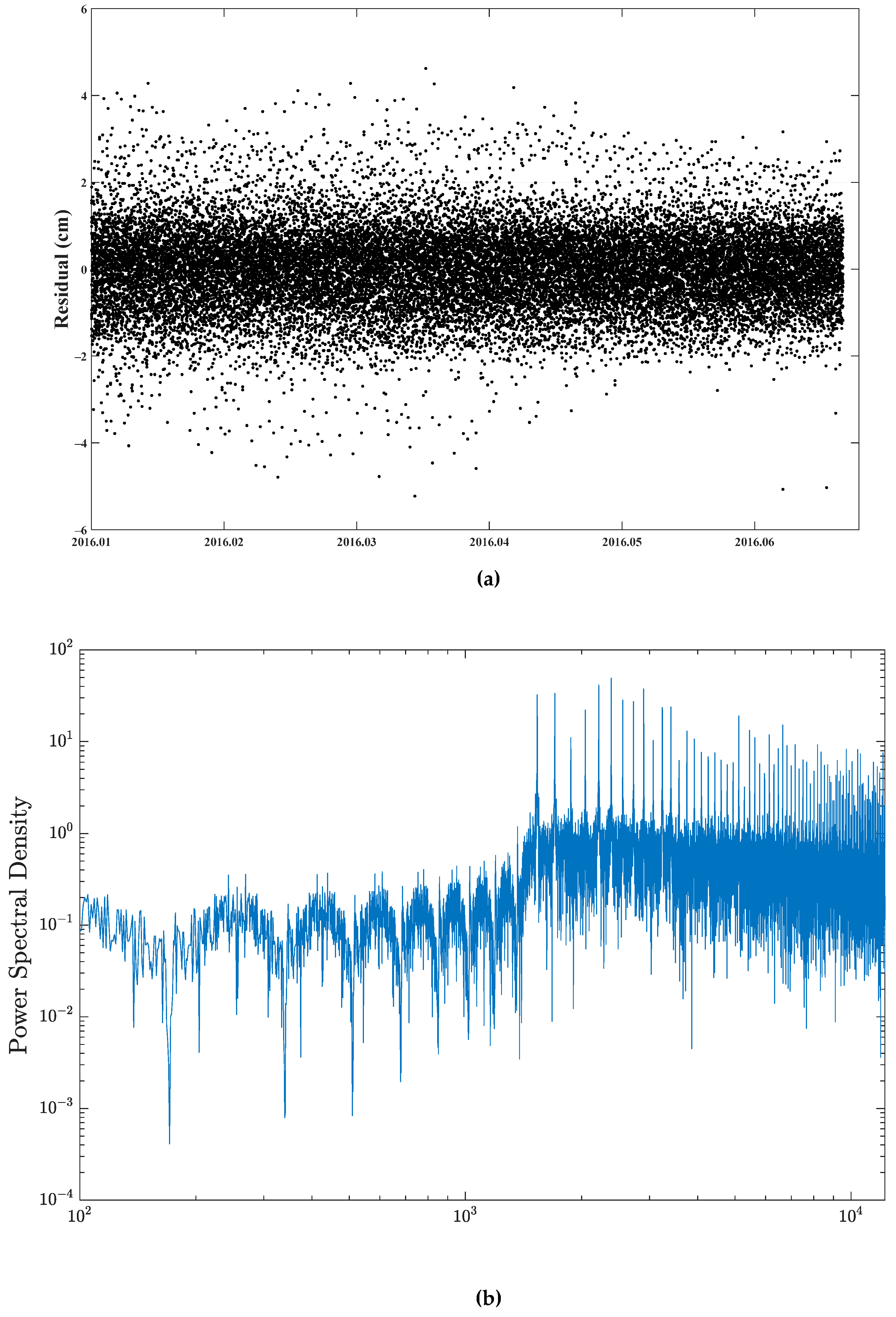
4.3. Noise Characteristic Analysis

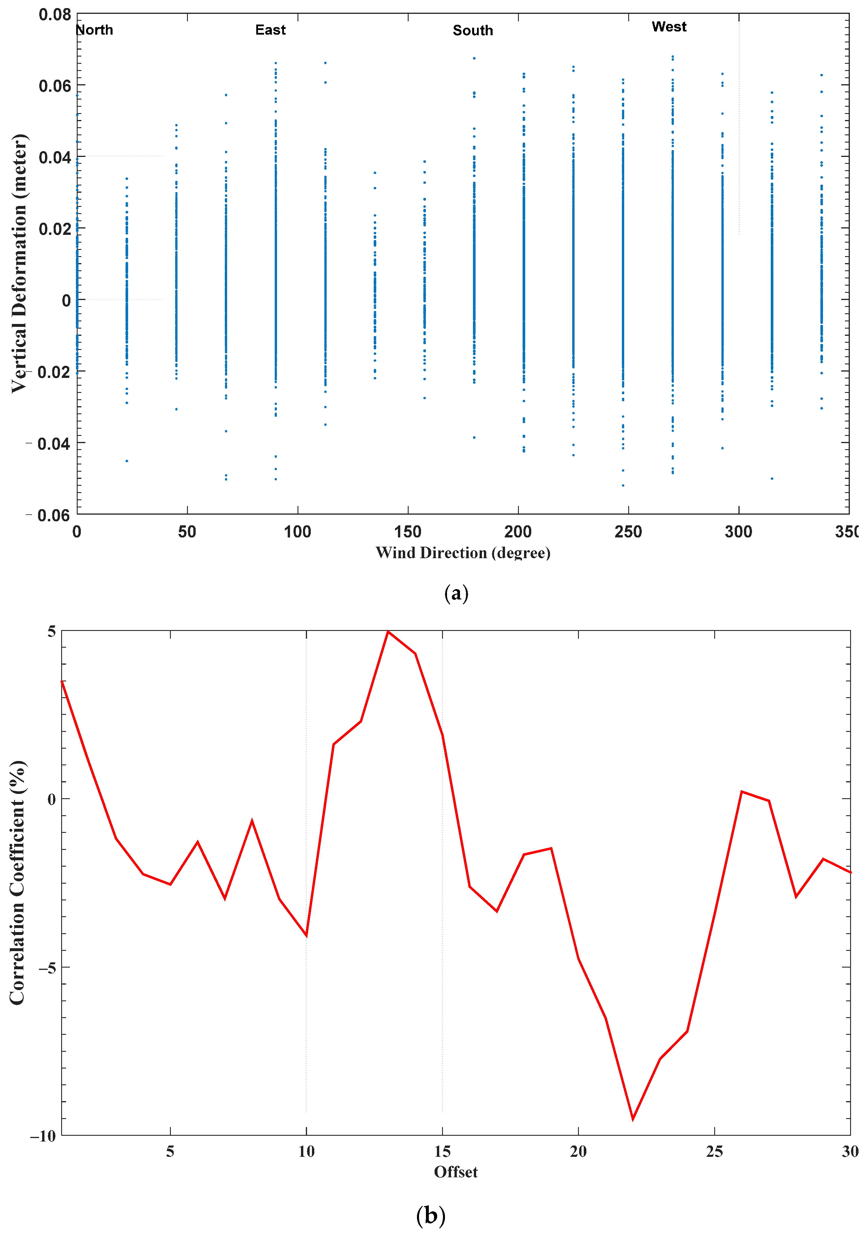
For the noise characteristic analysis by using residuals, the same dataset used in Section 4.2 is adopted. The linear trend, annual signal and its harmonics, daily signal and its harmonics through time domain are shown in Equation (6):

$$Residual=Z_{raw}-velocity·t-offset-{\sum }_{i=1}^2{A}_{i}sin\left({\omega }_i·t+{\phi }_i\right)-{\sum }_{j=1}^8{A}_{j}sin\left({\omega }_j·t+{\phi }_j\right).$$

(6)

The resulting residual time series is displayed in Figure 11a. The PSD values of residuals are shown in Figure 11b. It is clear that the slope of PSD tends to be 0, which indicates that white noise dominates in the residuals and other kinds of noise have nearly no effect. This also demonstrates that the white noise hypothesis of LSE is reasonable for the estimation of linear trends, annual signals and their harmonics, and daily signals and their harmonics. Also, there are still many signals that can be found through PSD, and this needs further research.

5. Discussion

Considering the specific location of the FRB, the NAD may lead to the drastic fluctuation of GVD. As shown in Figure 12, the North Atlantic Drift contributes to the moderate weather of Western Europe. As seen in Figure 8, the minimum air temperature in the winter is near $0°\text{C}$, while the maximum is less than $20°\text{C}$. The prevailing southwesterly trade wind is one of the major ways that the NAD affects the weather of Scotland, where the FRB is located. The wind speed can reach 50 mph in the winter, as shown in Figure 8. Considering that the wind speed data are sub-sampled, the actual maximum value of wind speed reached 70.2 mph on 29 January 2016. The humidity would also be significantly affected by the wind. Since the tower is 150 m above mean sea level, the warm trade wind in the winter would increase moisture evaporation and lead to the quick temperature change of the tower. This phenomenon is called wind chill [47], which means that the wind would accelerate the temperature change of the steel structure to be consistent with the ambient temperature. This can explain why the peaks of the GVD are highly consistent with the peaks of the wind speed in Figure 8 in the winter. Here, the GVD and wind speed data of 94 days from 30 December 2015 to 1 April 2016 are selected for analyzing their relationship. Cross-correlation analysis was carried out to find out the offset of two time series when a maximum coefficient is reached. A sliding window with a step of one day is used to calculate all the coefficients from 30 days before the maximum one is identified. It can be found from Figure 12 when the offset is one day the coefficient reaches to its maximum of 52.64% because the wind chill of steel is more significant with low temperature and high value of wind speed and humidity. Considering the noise effect in the time series, it can be concluded that the trade wind contributes to the structure temperature change, which further causes the seasonal vertical deformation of the tower in the winter. However, details about the wind chill of a steel structure are still unclear and need further research.

The wind direction is also an important factor that affects wind-induced responses. Here, the same dataset of 94 days from 30 December 2015 to 1 April 2016 is utilized for the study of the relationship between GVD and wind direction. Due to the resolution of the anemometer, the wind direction was measured at a $22.5°$ scale. The wind direction of the north is defined as $0°$ and other directions are defined with a clockwise direction successively, which means the east, south and west directions are defined as $90°$, $180°$ and $270°$, respectively. Figure 13a displays the GVD against wind direction. It can be seen that the GVD tends to be slightly scattered in the east and west, but this is not significant. A possible reason is that the lateral stability of the bridge is more readily affected by the wind-induced loadings. In the other directions, there is no clear dependence of the GVD on the wind direction since the FRB tower is stabilised by cables. The same cross-correlation analysis as in Figure 12 was carried out to find the offset of the GVD and wind direction when a maximum coefficient is reached, and the results are exhibited in Figure 13b. It is clear that the values of the cross-correlation are below 10%, which indicates a poor correlation between the GVD and the wind direction. Therefore, it can be concluded that the wind direction has limited effects on the 10-min mean vertical deformation of the tower.

In the summer, solar radiation contributes to the structure temperature; the differences between the structure temperature of the tower and ambient temperature would decrease compared with in the winter, and thus the amplitudes of the GVD and TED correlate relatively well with each other. However, the ambient temperature cannot be a proper replacement for the steel structure temperature of the tower. In the summer, due to different factors such as stronger solar radiation, higher air and surface temperature and heavier daily traffic, etc. affecting the GVD, in-depth research is required to further reveal the GVD mechanism.

Additionally, there seems to be a phase delay of ~30 degrees (about 30 days) between the GVD and TED time series, which can be explained as a shift process from the change of ambient temperature to the change of the steel structure temperature, which will further result in thermal expansion. For the semi-annual pattern, the amplitudes and phases of these two series cannot fit well with each other, which may indicate that the semi-annual signal in the GNSS vertical deformation time series is not related to thermal effects on the tower. Also, the difference between the steel structure temperature of the tower and the ambient temperature is another possible reason.

The mechanism of the daily and sub-daily signals is quite complicated without the support of traffic and meteorological data, including steel structure temperature, wind speed, wind direction etc. The amplitude results of daily signals of vertical deformation achieved by LSE display poor consistency with the relevant amplitude results of temperature data. However, the phase variation tendency of the vertical deformation and the temperature data are highly consistent from February 2016. The data selected from 1 January 2016 to 14 January 2016 demonstrate the poor daily periodicity of the temperature data, in which the NAD may play a role because of the large values of wind speed exhibited in Figure 8.

6. Conclusions

In this paper, we discussed the major factors affecting the vertical deformation of the southern supporting tower of the Forth Road Bridge in the UK, and attempted to reveal the relevant deformation mechanism with 33-month GNSS and 15-month meteorological data. A new measurement and data processing strategy is proposed in this paper, aimed at facilitating the signal extraction of vertical deformation time series.

From the estimation of linear deformation trend and the parameters of periodic signals, an accurate tower subsidence pattern is established to be 4.7 mm/year $\pm$ 0.1 mm. The amplitude of the annual signal is 9.3 mm $\pm$ 0.1 mm. A linear thermal expansion model with the coefficient of steel structure is used to simulate the thermal expansion deformation with the support of 15 months of meteorological data. The results show a high correlation of 98.9% in the amplitude of the annual signal, which demonstrates the dominant contribution of thermal expansion to the annual signals of the vertical deformation. For the daily signal analysis, it is difficult to determine any relationship between the amplitude of the daily vertical deformation and the temperature time series. However, the phase variation tendency of the vertical deformation and the temperature data show high consistency from February 2016, which demonstrates the effect of temperature on the daily signal.

Finally, the potential contribution of the NAD is discussed and the effects of wind speed and wind direction are also analysed. It is found that the warm trade wind in the winter may affect the wind chill of the steel structure of the tower and result in a difference between the steel structure and the ambient temperature of the tower that cannot be reflected when using the air temperature. The phase delay between the actual and simulated time series to some extent demonstrated the effect of the NAD-induced trade wind. At the same time, the poor consistency of the amplitude and the phase results of the daily signals in January 2016 also verify the effect of the trade wind.

This paper fails to make a more accurate simulation of the annual response and loading signals and attain the detailed parameters and mechanism of daily and sub-daily signals. More detailed meteorological and other relevant data sources are essential for the SHM to support a more accurate assessment of bridge conditions.

References

1. Estes, A.C. Bridge Maintenance, Safety Management, Health Monitoring and Informatics. Struct. Infrastruct. Eng. 2009, 5, 341. [Google Scholar] [CrossRef]
2. Larocca, A.P.C.; Schaal, R.E.; Santos, M.C.; Langley, R.B. Analyzing the dynamic behavior of suspension bridge towers using GPS. In Proceedings of the 19th International Technical Meeting of the ION Satellite Division—ION GNSS 2006, Fort Worth, TX, USA, 26–29 September 2006. [Google Scholar]
3. Chen, Z.; Zhou, X.; Wang, X.; Dong, L.; Qian, Y. Deployment of a Smart Structural Health Monitoring System for Long-Span Arch Bridges: A Review and a Case Study. Sensors 2017, 17, 2151. [Google Scholar] [CrossRef] [PubMed]
4. Meng, X. Real-Time Deformation Monitoring of Bridges Using GPS/Accelerometers. Ph.D. Thesis, University of Nottingham, Nottingham, UK, 2002. [Google Scholar]
5. Doebling, S.W.; Farrar, C.R.; Prime, M.B.; Shevitz, D.W. Damage Identification and Health Monitoring of Structural and Mechanical Systems from Changes in Their Vibration Characteristics: A Literature Review; Los Alamos National Laboratory: Los Alamos, NM, USA, 1996.
6. Ashkenazi, V.; Roberts, G.W. Experimental monitoring of the Humber Bridge using GPS. Proc. Inst. Civ. Eng.-Civ. Eng. 1997, 120, 177–182. [Google Scholar] [CrossRef]
7. Ren, W.-X.; Harik, I.E.; Blandford, G.E.; Lenett, M.; Baseheart, T.M. Roebling suspension bridge. II: Ambient testing and live-load response. J. Bridge Eng. 2004, 9, 119–126. [Google Scholar] [CrossRef]
8. Meng, X.; Dodson, A.H.; Roberts, G.W. Detecting bridge dynamics with GPS and triaxial accelerometers. Eng. Struct. 2007, 29, 3178–3184. [Google Scholar] [CrossRef]
9. Bao, Y.; Beck, J.L.; Li, H. Compressive sampling for accelerometer signals in structural health monitoring. Struct. Health Monit. 2011, 10, 235–246. [Google Scholar]
10. Zonta, D.; Esposito, P.; Pozzi, M.; Molignoni, M.; Zandonini, R.; Ming, W.; Daniele, I.; Daniele, P.; Glisic, B. Monitoring load redistribution in a cable-stayed bridge. In Proceedings of the 5th European Conference on Structural Control, Genova, Italy, 18–20 June 2012. [Google Scholar]
11. Curry, S.; Griffioen, P. Real-Time Kinematic GPS for Surveying: Centimeters in Seconds. In Proceedings of the American Society for Photogrammetry and Remote Sensing and America Congress on Surveying and Mapping Annual Convention, New Orleans, LA, USA, 15–18 February 1993; p. 109. [Google Scholar]
12. Meng, X.; Roberts, G.W.; Dodson, A.H.; Ince, S.; Waugh, S. GNSS for structural deformation and deflection monitoring: Implementation and data analysis. In Proceedings of the 3rd IAG/12th FIG symposium, Baden, Austria, 22–24 May 2006. [Google Scholar]
13. Hofmann-Wellenhof, B.; Lichtenegger, H.; Collins, J. Global Positioning System: Theory and Practice; Springer Science & Business Media: Berlin, Germany, 2012. [Google Scholar]
14. Brown, C.J.; Roberts, G.W.; Meng, X. A Tale of Five Bridges; the use of GNSS for Monitoring the Deflections of Bridges. J. Appl. Geod. 2014, 8, 241–264. [Google Scholar]
15. Celebi, M.; Sanli, A. GPS in pioneering dynamic monitoring of long-period structures. Earthq. Spectra 2002, 18, 47–61. [Google Scholar] [CrossRef]
16. Yang, J.; Li, J.B.; Lin, G. A simple approach to integration of acceleration data for dynamic soil–structure interaction analysis. Soil Dyn. Earthq. Eng. 2006, 26, 725–734. [Google Scholar] [CrossRef]
17. Psimoulis, P.A.; Stiros, S.C. Measuring deflections of a short-span railway bridge using a robotic total station. J. Bridge Eng. 2013, 18, 182–185. [Google Scholar] [CrossRef]
18. Sousa, J.J.; Hlaváčová, I.; Bakoň, M.; Lazecký, M.; Patrício, G.; Guimarães, P.; Bento, R. Potential of multi-temporal InSAR techniques for bridges and dams monitoring. Procedia Technol. 2014, 16, 834–841. [Google Scholar] [CrossRef]
19. Caldera, S.; Realini, E.; Barzaghi, R.; Reguzzoni, M.; Sansò, F. Experimental Study on Low-Cost Satellite-Based Geodetic Monitoring over Short Baselines. J. Surv. Eng. 2016, 142, 04015016. [Google Scholar] [CrossRef]
20. Sampietro, D.; Caldera, S.; Capponi, M.; Realini, E. Geoguard—An Innovative Technology Based on Low-cost GNSS Receivers to Monitor Surface Deformations. In Proceedings of the First Eage Workshop on Practical Reservoir Monitoring, Amsterdam, The Netherlands, 6–9 March 2017. [Google Scholar]
21. Li, H.-N.; Yi, T.-H.; Yi, X.-D.; Wang, G.-X. Measurement and analysis of wind-induced response of tall building based on GPS technology. Adv. Struct. Eng. 2007, 10, 83–93. [Google Scholar] [CrossRef]
22. Blewitt, G.; Lavallée, D.; Clarke, P.; Nurutdinov, K. A new global mode of Earth deformation: Seasonal cycle detected. Science 2001, 294, 2342–2345. [Google Scholar] [CrossRef] [PubMed]
23. Jiang, W.; Li, Z.; van Dam, T.; Ding, W. Comparative analysis of different environmental loading methods and their impacts on the GPS height time series. J. Geod. 2013, 87, 687–703. [Google Scholar] [CrossRef]
24. The Forth Bridges. Available online: https://www.theforthbridges.org/forth-road-bridge/facts-and-figures/ (accessed on 17 February 2018).
25. Transport Scotland. Available online: https://www.transport.gov.scot/publication/forth-replacement-crossing-environmental-statement/j11223-007/#22 (accessed on 17 February 2018).
26. Business Applications. Available online: https://artes-apps.esa.int/projects/showcases/monitoring-bridges-space (accessed on 17 February 2018).
27. Rizos, C. Alternatives to current GPS-RTK services and some implications for CORS infrastructure and operations. GPS Solut. 2007, 11, 151–158. [Google Scholar] [CrossRef]
28. Geng, J.; Shi, C. Rapid initialization of real-time PPP by resolving undifferenced GPS and GLONASS ambiguities simultaneously. J. Geod. 2016, 91, 361–374. [Google Scholar] [CrossRef]
29. Gil, H.; Park, J.; Cho, J.; Jung, G. Renovation of structural health monitoring system for Seohae bridge, Seoul, South Korea. Transp. Res. Rec. 2010, 2201, 131–138. [Google Scholar] [CrossRef]
30. Ogundipe, O.; Roberts, G.W.; Brown, C.J. GPS monitoring of a steel box girder viaduct. Struct. Infrastruct. Eng. 2014, 10, 25–40. [Google Scholar] [CrossRef]
31. Bogusz, J.; Klos, A. On the significance of periodic signals in noise analysis of GPS station coordinates time series. GPS Solut. 2016, 20, 655–664. [Google Scholar] [CrossRef]
32. Williams, S. The effect of coloured noise on the uncertainties of rates estimated from geodetic time series. J. Geod. 2003, 76, 483–494. [Google Scholar] [CrossRef]
33. Santamaría Gómez, A.; Bouin, M.N.; Collilieux, X.; Woeppelmann, G. Correlated errors in GPS position time series: Implications for velocity estimates. J. Geophys. Res. Solid Earth 2011, 116. [Google Scholar] [CrossRef]
34. Langbein, J. Estimating rate uncertainty with maximum likelihood: Differences between power-law and flicker–random-walk models. J. Geod. 2012, 86, 775–783. [Google Scholar] [CrossRef]
35. Langbein, J. Noise in GPS displacement measurements from Southern California and Southern Nevada. J. Geophys. Res. Solid Earth 2008, 113. [Google Scholar] [CrossRef]
36. King, M.A.; Williams, S.D. Apparent stability of GPS monumentation from short-baseline time series. J. Geophys. Res. Solid Earth 2009, 114. [Google Scholar] [CrossRef]
37. Davis, J.L.; Wernicke, B.P.; Tamisiea, M.E. On seasonal signals in geodetic time series. J. Geophys. Res. Solid Earth 2012, 117. [Google Scholar] [CrossRef] [Green Version]
38. Jiang, W.; Zhou, X. Effect of the span of Australian GPS coordinate time series in establishing an optimal noise model. Sci. China Earth Sci. 2015, 58, 523–539. [Google Scholar] [CrossRef]
39. Amiri-Simkooei, A.R. Noise in multivariate GPS position time-series. J. Geod. 2009, 83, 175–187. [Google Scholar] [CrossRef]
40. Wang, J.; Meng, X.; Qin, C.; Yi, J. Vibration Frequencies Extraction of the Forth Road Bridge Using High Sampling GPS Data. Shock Vib. 2016, 2016. [Google Scholar] [CrossRef]
41. Zhou, G.D.; Yi, T.H. Thermal Load in Large-Scale Bridges: A State-of-the-Art Review. Int. J. Distrib. Sens. Netw. 2013, 9. [Google Scholar] [CrossRef]
42. Dong, D.; Fang, P.; Bock, Y.; Cheng, M.K.; Miyazaki, S.I. Anatomy of apparent seasonal variations from GPS-derived site position time series. J. Geophys. Res. Solid Earth 2002, 107. [Google Scholar] [CrossRef]
43. Hill, E.M.; Davis, J.L.; Elósegui, P.; Wernicke, B.P.; Malikowski, E.; Niemi, N.A. Characterization of site-specific GPS errors using a short-baseline network of braced monuments at Yucca Mountain, southern Nevada. J. Geophys. Res. Solid Earth 2009, 114. [Google Scholar] [CrossRef]
44. Yang, L.; Wang, G.; Bao, Y.; Kearns, T.J.; Yu, J. Comparisons of ground-based and building-based CORS: A case study in the region of Puerto Rico and the Virgin Islands. J. Surv. Eng. 2015, 142, 05015006. [Google Scholar] [CrossRef]
45. Holický, M.; Marková, J. Thermal Actions. 2008. Available online: http://eurocodes.jrc.ec.europa.eu/doc/WS2008/Holicky_Markova_2008.pdf (accessed on 22 February 2018).
46. Roy, R.; Agrawal, D.K.; Mckinstry, H.A. Very Low Thermal Expansion Coefficient Materials. Ann. Rev. Mater. Res. 1989, 19, 59–81. [Google Scholar] [CrossRef]
47. Wikipedia. Available online: https://en.wikipedia.org/wiki/Wind_chill (accessed on 17 February 2018).
Figure 1. The geo-location of the FRB.
Remotesensing 10 00364 g001
Figure 2. Deployments of GNSS receivers of the GeoSHM FS Project: (a) deployments of GNSS receivers on the FRB; (b) GNSS receiver on the South Tower (SHM4); (c) reference station (SHM1).
Remotesensing 10 00364 g002
Figure 3. Flow chart of data processing strategy.
Remotesensing 10 00364 g003
Figure 4. The 3D 10-min average deformation time series.
Remotesensing 10 00364 g004
Figure 5. PSDs of the vertical deformation time series.
Remotesensing 10 00364 g005
Figure 6. The black points represent the vertical deformation time series that excluded the effect of linear velocity, and the red curve represents the fluctuation of annual signal.
Remotesensing 10 00364 g006
Figure 7. The assessment about the effect of horizontal deformation on vertical deformation.
Remotesensing 10 00364 g007
Figure 8. The first subplot above displays the observed GVD and the modelled TED time series; the second subplot displays the temperature and average wind speed data.
Remotesensing 10 00364 g008
Figure 9. (a) The upper subplot displays the 10-min averaged vertical deformation time series, the middle subplot displays the amplitude results of the daily signals of vertical deformation (blue) and temperature (red), and the lower subplot exhibits the phase results of the daily signals of vertical deformation (blue) and ambient temperature (red). (b) The PSD of temperature data with a length of 15 months.
Remotesensing 10 00364 g009
Figure 10. Blue displays the real vertical deformation time series; black represents the fitting vertical deformation time series using the parameters achieved by LSE of Equation (5); and red represents the real air temperature data (a,b).
Remotesensing 10 00364 g010
Figure 11. (a) The value of the residual; (b) the PSD of the residual.
Remotesensing 10 00364 g011
Figure 12. The correlation coefficient between GVD and wind speed with different offsets.
Remotesensing 10 00364 g012
Figure 13. The relationship between the vertical deformation and wind: (a) GVD against wind direction; (b) the correlation coefficient between GVD and wind angle with different offsets.
Remotesensing 10 00364 g013