An Exploration of Some Pitfalls of Thematic Map Assessment Using the New Map Tools Resource


1
Swedish University of Agricultural Sciences, Southern Swedish Forest Research Centre, SE-23053 Alnarp, Sweden
2
International Institute for Applied Systems Analysis (IIASA), Center for Citizen Science and Earth Observation, Schlossplatz 1, 2361 Laxenburg, Austria
*
Author to whom correspondence should be addressed.
Remote Sens. 2018, 10(3), 376; https://doi.org/10.3390/rs10030376
Submission received: 23 January 2018
/
Revised: 13 February 2018
/
Accepted: 18 February 2018
/
Published: 1 March 2018
Abstract
:A variety of metrics are commonly employed by map producers and users to assess and compare thematic maps’ quality, but their use and interpretation is inconsistent. This problem is exacerbated by a shortage of tools to allow easy calculation and comparison of metrics from different maps or as a map’s legend is changed. In this paper, we introduce a new website and a collection of R functions to facilitate map assessment. We apply these tools to illustrate some pitfalls of error metrics and point out existing and newly developed solutions to them. Some of these problems have been previously noted, but all of them are under-appreciated and persist in published literature. We show that binary and categorical metrics, including information about true-negative classifications, are inflated for rare categories, and more robust alternatives should be chosen. Most metrics are useful to compare maps only if their legends are identical. We also demonstrate that combining land-cover classes has the often-neglected consequence of apparent improvement, particularly if the combined classes are easily confused (e.g., different forest types). However, we show that the average mutual information (AMI) of a map is relatively robust to combining classes, and reflects the information that is lost in this process; we also introduce a modified AMI metric that credits only correct classifications. Finally, we introduce a method of evaluating statistical differences in the information content of competing maps, and show that this method is an improvement over other methods in more common use. We end with a series of recommendations for the meaningful use of accuracy metrics by map users and producers.
1. Introduction
Maps are in increasing demand for many business, government, and humanitarian applications. It is also increasingly recognized that map quality matters, a view reflected in the guidelines for many map production contracts that are issued by governments and other organizations [1]. However, stated accuracy requirements do not always guarantee high-quality or useful maps. Poorly constructed requirements may allow map producers to satisfy map commissioners’ accuracy standards with a product that is not acceptable for map users. Map users, in turn, face a complex series of decisions when choosing a map product for their application [2]. Central to the decision-making process is the question of map value [3], which itself depends upon the relative accuracy of maps under consideration and whether these differences are either statistically or practically different [4]. Map producers need to show to potential users and customers that their maps are of high quality; accuracy assessment is central to this process. Those who commission maps (such as government agencies) with a view toward diverse potential uses also have a stake in map assessment, and increasingly put accuracy requirements on producers. All of these stakeholders have an interest in accuracy assessment, but there are many ways to go about this process. In this paper, we focus on some pitfalls of choosing and implementing accuracy metrics. However, accuracy does not provide a complete picture of map quality, and we demonstrate some reasons why broader information-based metrics should be considered.
There are many metrics for assessing maps, and most thematic map products have been validated using at least one of these. However, this process is beset by many under-recognized pitfalls, even if the maps being compared report the same metrics. Each index has particular advantages and drawbacks. Over three decades of literature dispute, which metrics are appropriate under which circumstances, and even whether certain methods have any value at all [5,6,7,8]. Metrics for assessing maps have been reviewed comprehensively elsewhere [9], and we do not attempt to repeat this exercise. Here, we take the view that accuracy and quality are not the same thing, but rather that accuracy is one aspect of quality. We discuss some specific problems that arise in map assessment and how to avoid them. As has been previously shown (but not consistently recognized), the choice of classes in a legend, and in particular, the extent of their aggregation, has a big impact on overall accuracy [10], a point we further elaborate in this paper. Accuracy guidelines are sometimes presented in a completely nonsensical way. For instance, the “Mapping Guide for a European Urban Atlas” thematic accuracy guidelines call for “Minimum overall accuracy for level 1 class 1 “Artificial surfaces”: 85%” [1]. This shows confusion between overall and class-level accuracy, and as we demonstrate below, these types of class-specific measures can be biased by information that has nothing to do with the cover class under consideration. To help map producers and users navigate these challenges, we introduce ‘Map Tools’, a new web-based resource (tool.laco-wiki.net) for calculating map quality metrics and use it to illustrate some challenges of map assessment and comparison with a series of vignettes based on hypothetical map validation examples. Finally, we present solutions, both new and previously published, to these problems.
2. Thematic Map Quality Metrics
What are frequently called ‘accuracy metrics’ for maps and other purposes can be computed from a square confusion matrix (also known as an ‘error matrix’) in which rows typically represent classified categories, and columns reference categories (note however that some authors transpose the rows and columns of the error matrix [11]). Each cell contains the number of points (or the proportion of points) with a particular combination of observed and reference land-cover categories. Correct classifications are on the matrix diagonal; incorrect pixels are off-diagonal [12].
Accuracy metrics are intended for use either at a map-wide level in which an entire map is distilled into a single number, or at a category-specific level where each cover class is evaluated individually. Map-level metrics can be made into category-level statistics by collapsing the error matrix into a binary matrix for each category (a matrix that contains two classes, one for the category of interest, and another for everything else), and then calculating that metric on those binary matrices. Conversely, a category-level metric can be converted to a map-wide metric by averaging the categories’ scores, weighted by the categories’ proportions on the map, although this is not appropriate or meaningful for all metrics. In some cases map-wide and category-level versions of a metric have completely different names. We mostly focus on map-wide metrics in this paper, although we also address some types of category-level metrics. That we mention a particular metric in this section should not be taken as an implied endorsement. As we show later in the paper, many of these metrics are subject to misuse and some are unlikely to have any appropriate use at all.
The most basic metric, overall accuracy, is the proportion of pixels or points that are classified correctly. That is simply the sum of the confusion matrix diagonal divided by the sum of the entire confusion matrix. Although this is a map-level metric, it has a close relative at the category level, the “portmanteau” accuracy [13]. While overall accuracy is intuitive to grasp, it can be misused or misleading. The accuracy calculation is dependent on the choice of validation pixels; if these are not representative of the landscape, the computed accuracy value is biased [11]. This problem can be corrected through weighting by the observed frequency of each land cover type (see [11], Equation 19). Overall accuracy is often criticized for making no correction for the number of pixels that can be expected to be classified correctly by chance alone [14]. The ‘kappa’ metric attempts to solve the problem of random chance agreement; it was introduced to account for the chance agreement of observed and reference categories [15]. Kappa can also be applied as a category-level metric, although it is less commonly used this way [16]. One attractive feature of kappa is that the formula for its variance is well known, allowing statistical testing of differences between maps’ accuracies [12], although in principle this can be done for other metrics. However, kappa and related metrics have been fiercely criticized for many reasons, most fundamentally for not adding any new information to basic accuracy assessment [8].
User’s and producer’s accuracies are two metrics that provide related perspectives on class-level accuracy. User’s accuracy is the proportion of points of a given classification that are validated to actually be in that class. Producer’s accuracy is the proportion of points in a reference category that were classified that way. Both of these metrics are applied on a per-category basis, although see below for discussion of their map-wide application. Producer’s accuracy is sometimes called the ‘sensitivity’ [17]. Another metric called ‘specificity’ complements sensitivity [17]. Specificity is essentially the producer’s accuracy of classification outside of a particular category. In other words, it is the proportion of map pixels correctly classified in the ‘no’ category of a binary map.
Quantity disagreement’ and ‘allocation disagreement’ are a pair of metrics recently proposed as an alternative to kappa-family indices [8]. These break overall error (equal to 1 − overall accuracy) into two parts. The authors who introduced these terms define quantity disagreement as “the amount of difference between the reference map and a comparison map that is due to the less than perfect match in the proportions of the categories” and allocation disagreement as “the amount of difference between the reference map and a comparison map that is due to the less than optimal match in the spatial allocation of the categories, given the proportions of the categories in the reference and comparison maps” [8]. Two recently introduced metrics further divide the allocation disagreement into components of “exchange” and “shift” [18]. The sum of allocation disagreement and quantity disagreement is equal to overall error. Formulas for these metrics on both category-specific and map-wide levels are given in [8,18].
A final family of metrics stems from information theory and evaluates average mutual information (AMI), or the amount of information shared between a set of classified and reference points [19]. This can be thought of as a measure of how much information the mapped classes provide about the actual classes on the landscape, and how much information is conveyed in the correspondence between the mapped and true classes. For instance, all else being equal, a map with more classes contains more information. Along the scale from less to more information-rich would be a simple map with one class containing all of the forested land, a medium-complexity map that divides this into evergreen and deciduous classes, and a detailed map that has many classes for the dominant tree species in a forest parcel. There are versions of this metric that take perspectives analogous to the user’s or producer’s accuracy, and can be computed at the map-wide or category level [19]. These values are not limited to the typical range of 0 to 1 and depend on the base of the logarithm used in the calculation. In this paper, we use a base 2 logarithm, for results in units of ‘bits’, although they can be converted to base e or base 10 units by multiplying by loge(2) = 0.693 or log10(2) = 0.301. AMI can also be normalized to the theoretical maximum amount of information possible given the distribution of categories in a map. This is known as the proportional (or percentage) average mutual information (PAMI [19]). PAMI is the same regardless of logarithm base.
In this paper, we use Map Tools to highlight ways in which these error metrics can be, and are often misused when evaluating thematic map accuracy. We point out difficulties such as (1) how certain metrics can be manipulated by inflating the number of true negatives in an error matrix, (2) using cross-category averages of user’s and producer’s accuracies, (3) testing for significant differences in thematic map accuracy using the variance of the kappa metric, and (4) comparing accuracy metrics of maps with different legends. Finally, we introduce methods of statistically comparing information-theory-based metrics that add value to these already useful indices.
3. The Map Tools Website
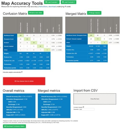
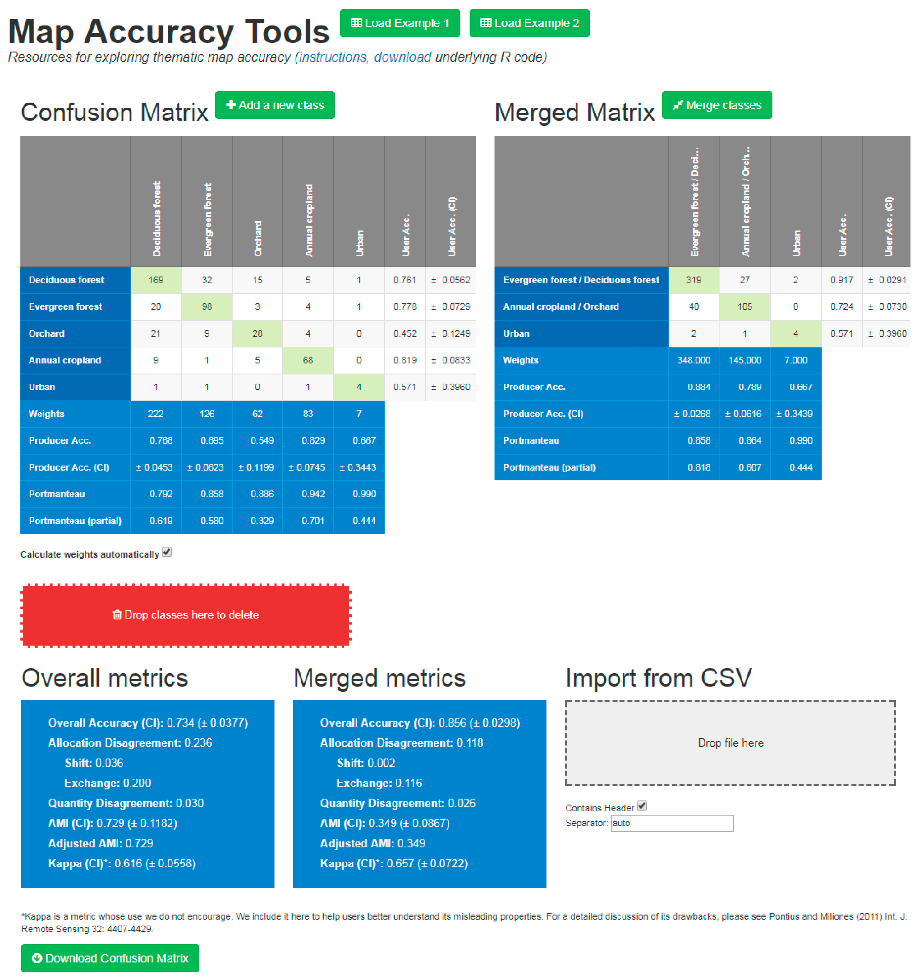
The Map Tools website (tool.laco-wiki.net) provides a suite of thematic map accuracy resources in an easy-to-use format. All of the functionality described below is based on underlying code that is written in the statistical language R [20], which is available at the Map Tools website. All of the metrics are based on error matrices that may be entered manually, copied, and pasted, or imported as comma separated (.csv) files. The website automatically calculates multiple accuracy metrics, both at the overall and categorical levels. For many metrics, a variance can also be computed to allow for statistical comparisons between maps. The variance can either be returned raw, which has uses such as testing differences among maps, or as a 95% confidence interval, which more intuitively represents the precision in the same units as the metric itself. The metrics can be calculated under simple random sampling or with stratification by mapped class (note that more complex stratifications, for instance, focusing on areas of likely mapping errors, are not currently supported). In the case of a stratified design, the mapped classes’ relative covers are entered as weighting factors. The importance of using correct weighting based on sampling probabilities is well discussed elsewhere [21], but can easily be illustrated using this feature. Simply change the weights, for instance from the default values to the situation where each class has equal area, and note how much the overall metrics change. The Map Tools website has a function to allow for easy exploration of how merging classes affects accuracy measures. This is done by clicking on the ‘Merge Classes’ buttons and using a drag and drop menu to group the categories of the original error matrix. An aggregated error matrix is automatically produced and displayed next to the original matrix along with accuracy statistics for the merged matrix (see Figure 1).
4. Demonstrations of Some Under-appreciated Features of Accuracy Metrics
In this section, we use Map Tools to demonstrate some important but under-appreciated properties of map accuracy metrics. We also develop some new procedures for map accuracy assessment useful for producers and users of maps. Many of our following demonstrations are based on a hypothetical error matrix of 500 randomly sampled points, as seen in Table 1. While this matrix describes a simple landscape map with only five cover categories, its simplicity serves to illustrate properties of accuracy metrics that may be less obvious in more complex maps. This matrix is loaded into the Map Tools website by default, and all of the following examples can be replicated with the help of the tools found there. This matrix can also be loaded by clicking on the ‘Load Example 1’ button at the top of the screen.
4.1. True Negative Validations Inflate Some Categorical Accuracy Metrics
Category-level accuracy metrics are misleading if they show apparent improvement when additional points not in that category are correctly classified. This problem does not apply only to binary maps. It can arise when categorical metrics are computed by effectively collapsing an error matrix into a binary matrix, and remaining classes are collected into an ‘everything else’ class. This presents the possibility of manipulating the metric by inflating the number of true negatives, particularly for categories occupying only a small proportion of a landscape. We illustrate this situation by collapsing the above error matrix into a binary evaluation of urban and non-urban cover. This example can be demonstrated on the website by loading example 1 and merging the corresponding classes, as seen in Table 2.
Here, the overall accuracy is (4 + 491)/500 = 99.0%. However, if there were fewer points correctly identified as non-urban cover, this value would be radically lower. Thus, most of the information contained in the figure of 99.0% has nothing to do with the category of interest. At least one published accuracy metric, the ‘partial portmanteau’ accuracy [13], also known as the ‘figure of merit’ [22], is robust to this source of bias. The basic ‘portmanteau’ accuracy is simply overall accuracy computed on a matrix collapsed to a presence/absence matrix of the cover type of interest [13], the same calculation that gave the value of 99.0% value above. Partial portmanteau accuracy eliminates true negatives (the number 491 in our example) from the calculation, so is the number of correctly mapped points in a category, divided by the total number of points mapped or validated in a category. In our example, this value comes to 4/(3 + 4 + 2) = 44.4%.
Some categorical accuracy metrics (e.g., user’s and producer’s accuracy/sensitivity) avoid inflation from true negatives simply because true negatives are not part of their calculations. Many other metrics are susceptible to this problem, including the previously mentioned portmanteau (but not the partial portmanteau) and specificity. These and other metrics that include true negatives will necessarily approach 100% for increasingly rare mapped classes.
4.2. Map-Wide Averages of User’s and Producer’s Accuracies Are not Meaningful
User’s and producer’s accuracies quantify the proportion of points classified in a category that are validated in that category and vice versa. It might seem desirable to have this information aggregated from the category to the map level. However, as we show below, and has been mentioned in at least one previous publication [23], mean user’s, and producer’s accuracies are both equal to overall map accuracy when the averaging is weighted by the classified (user’s) or reference (producer’s) category frequencies. If the categories are averaged without weighting, the values obtained can differ from overall accuracy. However, it is unclear what meaning that these averages have when all cover classes, from very rare to the most common, are weighted equally. Even so, it is not hard to find published examples of averaged user’s or producer’s accuracies ([24,25,26]). Note that in some cases, the unweighted mean producer’s accuracy of a binary matrix is sometimes called the ‘balanced accuracy rate’ ([25]).
Here, we show that average user’s accuracy, when weighted by user’s proportion of points in each cover class, is equivalent to overall accuracy. Analogous logic applies to mean producer’s accuracy. Let Eij be an N by N error matrix with rows i = 1, …, N corresponding to counts of map classifications in category i, and columns j = 1, …, N to map validations in category j; Ei indicates all of the values in row i of the matrix, and Ej the entries in column j. When i = j, a classification is considered correct. Overall accuracy (This assumes a random sampling design, i.e. that the proportions in this matrix represent the true landscape proportions; corrections for different sampling designs are available elsewhere) is equal to the proportion of classifications on the error matrix diagonal [9]:
User’s accuracy is the proportion of category i that is correctly classified:
The proportion (from the user’s perspective) of points classified in each category i is given by:
Thus, the average user’s accuracy, when weighted by categorical proportions is identical to overall accuracy:
This result can also be demonstrated empirically with R code available from the Map Tools website. Take example the example matrix in Table 1. It has an overall accuracy of 73.4%. The average of the five categories’ user’s accuracy values is 67.6%. However, inspecting the individual values, one notes that the more common categories (deciduous forest, evergreen forest, and cropland) all have an above-average user’s accuracy. When weighted by the proportion of points that are classified into each category, the mean user’s accuracy is found to be 73.4%, the same as the overall accuracy. The same can be shown for the producer’s accuracy.
4.3 Combining Categories Shows Misleading Increases in Overall Accuracy and Kappa, but not AMI
When comparing competing maps can be done in a variety of ways [2,3,4], but in the absence of specific values that are associated with different types of errors [3], overall accuracy is often used to compare competing maps [27,28,29]. However, competing maps rarely share a common legend. In this case such comparisons may be misleading [6,30]. Land-cover maps vary widely in their number of categories, ranging from two (for instance the urban/non-urban example above) to at least 44 in CORINE [31]. If a map has more categories, it may contain more information about land cover than a similar map with fewer categories, even if it has a lower overall accuracy [32]. However, we are unaware of any published method to make fair comparisons between the overall accuracy of such maps. Even when two maps seemingly share a category, definitions can differ, for instance, in the minimum tree cover or canopy height to qualify as a forest [21]. Although a few papers have noted that different land cover categories complicate map comparisons ([6,23]), little consideration has been paid to the validity of such comparisons or to the circumstances in which fair comparisons can actually be made.
When a new map is created by combining categories of another map, it has been shown that the overall accuracy of the new map must be equal to or better than the original map [10]. While this result makes intuitive sense, it is unfortunately underappreciated, perhaps because it was originally articulated for maps depicting cover change. However, it applies to all circumstances where map categories are aggregated, not just to maps of cover change. As an example, consider what would happen if the ‘evergreen forest’ and ‘deciduous forest’ categories from the hypothetical error matrix (Table 1) were merged into a single ‘forest’ category. All of the points classified as the wrong kind of forest are now correctly classified, while there is no way for correct points to become incorrect. This raises the overall accuracy from 73% to 94%.
The impact of class aggregation differs widely depending on which accuracy metric is used. To demonstrate this, we applied four class aggregation scenarios to two hypothetical error matrices. The first matrix is the one used in previous examples (Table 1; Example 1 on the website). The second is similar, but differs in having a more random distribution of errors among the categories—rather than evergreen forest being most commonly confused for deciduous forest, the errors are more evenly distributed among all of the categories (Table 3; this is Example 2 on the website). Six map-wide error metrics were calculated for these two matrices under four different scenarios: (1) no aggregation (all five categories); (2) aggregated to three categories: forest (deciduous forest and evergreen forest), agriculture (orchard and annual crops), and urban; (3) aggregated to a different set of three categories: trees (deciduous forest, evergreen forest and orchard), annual crops, and urban; and, (4) aggregated to two categories: urban and non-urban.
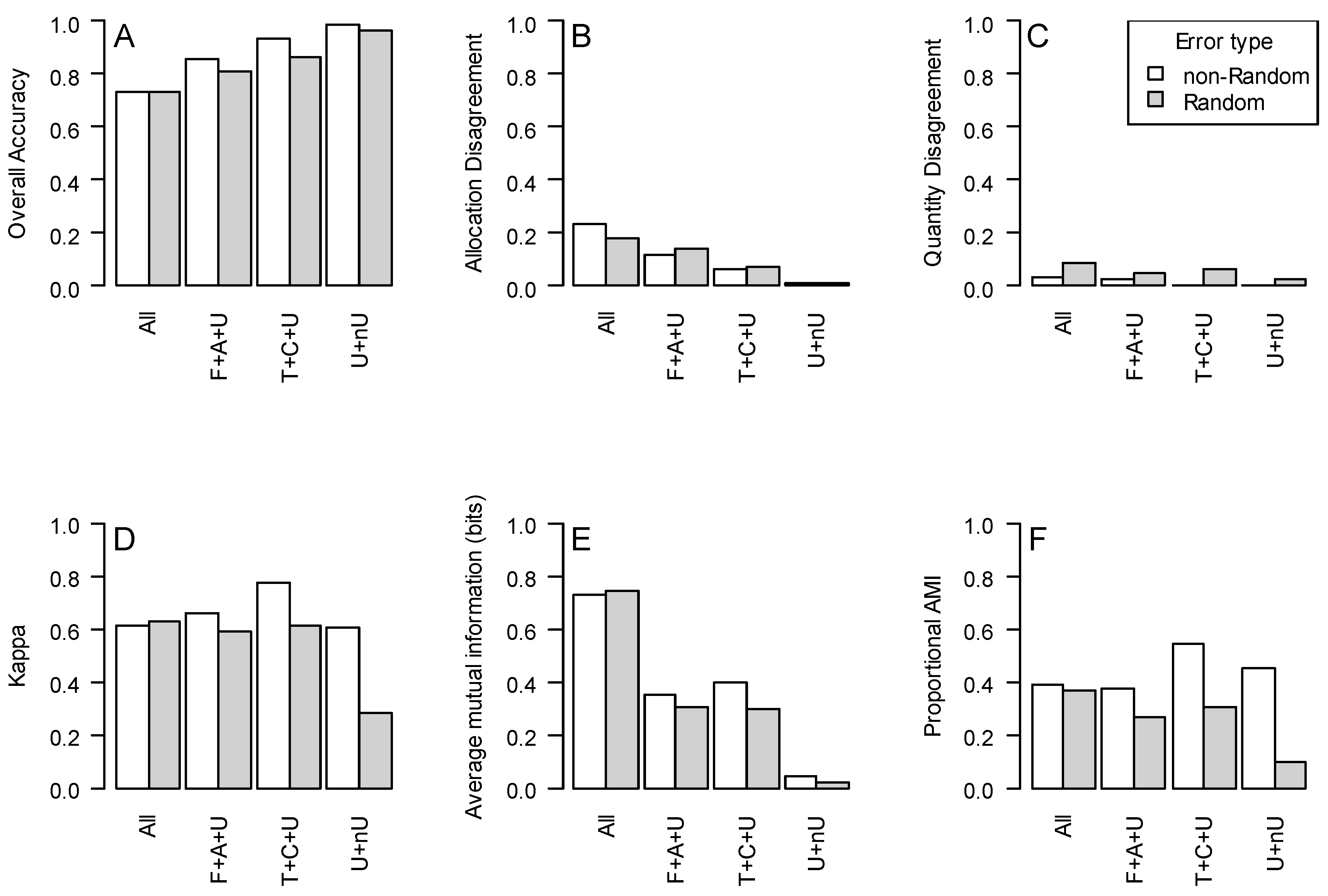
Overall accuracy increased from 73.4% in the original map up to 99% in the binary urban/non-urban map (Figure 2A). Allocation and quantity disagreement showed a very similar pattern to overall accuracy (Figure 2B—note the pattern appears reversed because it is a measure of disagreement among the classified and reference points, rather than agreement as in overall accuracy). Quantity disagreement was an extremely small part of the overall error in these simulations since the relative proportions of the cover classes remained little changed, especially in the non-random error scenario (Figure 2C). Unlike overall accuracy, kappa proved robust to the aggregation of categories when error was random, except for the most extreme scenario (the urban/non-urban map). However, when aggregation was nonrandom, kappa increased substantially for some aggregation scenarios (Figure 2D). Unlike all of the other metrics evaluated, average mutual information (AMI) indicated a consistent worsening of the maps when categories were aggregated (Figure 2E). AMI gave slightly higher values when errors were biased toward similar classes, although the score was still much below the unaggregated map (Figure 2E). In contrast, proportional AMI (PAMI—sometimes also called ‘standardized AMI’) had a pattern similar to kappa, with a tendency toward improvement when the mapping errors were non-random, and toward worsening when the errors were more random among classes (Figure 2F). This is due to the informational advantage of having more classes and is not reflected by PAMI; this advantage is removed because the AMI value is divided by the highest possible AMI score when standardizing.
One potential drawback of AMI is that it is not a measure of agreement. However, this is less of a problem than one might expect. The fundamental issue here is that in this context, AMI is a measure of predictability of true classes given mapped classes. Thus, it is possible to have a high AMI score on a map that is entirely incorrect. Such a map can be produced by switching the class labels on an otherwise perfect map. The overall accuracy and categorical accuracies would all be 0, but the AMI would be high because it is easy to predict the true class from the (incorrect) mapped class. To contend with this problem, we created an adjusted AMI metric (see the ami.adj() function in our online code library) that only counts positive contributions from on-diagonal cells of the error matrix. This removes any contribution from predictable but wrong classifications. We performed these calculations for the scenarios above, and the result is visually indistinguishable from Figure 2E; adjusted AMI values were identical for the non-random error scenarios, and showed either no change or a small decrease of between 0.63–2.33% in the random error scenario. When a confusion matrix contains enough error for AMI to benefit from misclassification, user, and/or producer accuracies for the affected classes will also be very low, emphasizing the importance of not interpreting any metric in a vacuum.
The patterns noted above have different consequences for different practitioners. Map producers may be interested in AMI if they create maps with more detailed legends than competing products. As demonstrated above (Figure 2A), the disaggregation of categories leads to lower overall accuracy, but AMI will demonstrate the benefits of any additional information imparted by the detailed legend. For organizations commissioning maps, specifying a required AMI in situations where the precise legend is left to the decision of the producer. Map users may have less need for AMI. If their intended use is focused on one or a few classes of the map, then class-level accuracies are likely more informative, particularly if the costs of specific types of mapping errors are known.
4.4. The Misleadingness of Statistical Kappa Comparisons
A formula for kappa’s variance is well known, allowing for the calculation of statistical significance of differences between two error matrices. However, this property can be extremely deceptive. Under some circumstances, two error matrices that are derived from the same underlying data appear to be significantly different. To demonstrate this, we return to two error matrices used in the previous example—(A) the unaggregated five-class matrix seen in Table 1, and (B) the matrix aggregated to three classes—woody vegetation, annual crops, and urban (seen in the right side of Figure 1). The original matrix has κA = 0.616, with var(κA) = 0.00081. The aggregated error matrix has κB = 0.657 and var(κB) = 0.00136. To account for possible covariance between the two kappa scores, we use the largest possible estimate of . The z-score of the difference between these two values is . The probability of getting a normally-distributed value greater than this by chance is p = 0.00671 (one tailed) or p = 0.0134 (two tailed), values considered to indicate moderately strong evidence by most standards. This apparently robust improvement in the map’s accuracy (as seen in Figure 2D—the difference between the ‘All’ and ‘T + C + U’ matrices) is actually the result of the loss of information.
4.5. How to Calculate the Statistical Significance of AMI Differences
Because of the many well-known shortcomings of kappa [8], it is desirable to have an alternative way to statistically compare map accuracy that does not rely on intuitive feelings about their differences. Here, we show that such calculations are also possible for AMI. To calculate the significance of differences among AMI values, it is necessary to estimate the variance of AMI. Fortunately, this result is available in the signal processing literature and does not have to be derived anew, although we are unaware of previous examples applying it to map assessment. Following our above notation, the variance of AMI under unstratified random sampling can be estimated as [33]:
where Ei,j is an error matrix of counts (as above), and the total number of validated points is n = ΣEi,j. With this information, it is possible to calculate a z-score for the difference between AMI for two matrices (A and B), which can then be used to calculate something akin to a p-value, analogous to the example with kappa:
To demonstrate the use of these formulas, we revisit the hypothetical error matrices used in the kappa comparison example from the previous section. The error matrix with five cover classes has a higher AMI (0.729) than the three-class matrix (0.399). Using the computed variances of AMI for these matrices, we find a z-score of 3.037, equivalent to p = 0.00239 (two-tailed). This stands in contrast to the difference in the opposite direction seen in the kappa example and correctly reflects the loss of information when classes are aggregated.
5. Recommendations
This paper has introduced the Map Tools website and used it to demonstrate some ways in which commonly used map accuracy metrics can be misinterpreted or misused, resulting in the loss of information that would otherwise inform map evaluations. Although papers detailing good practices for working with map accuracy are available and widely cited [34,35], some of these issues have not, to our knowledge, been noted previously. Others have been discussed in the literature, but remain sources of confusion in published studies [24,25,26]. For this reason, the examples that are presented here are a useful clarification of commonly held misconceptions. Some of these situations lend themselves to simple fixes; others are harder to contend with. In the remainder of this paper we discuss these accuracy reporting recommendations for producers and users of thematic maps.
Recommendation 1: Report raw error matrices and weight-corrected probability matrices. For map producers or others validating maps, validation reports should avoid throwing away or hiding potentially useful information. Most fundamentally, this means that reporting raw error matrices (counts, or proportions plus sample sizes to allow the reconstruction of counts) is essential, as is reporting precise details of the sampling design (were categories sampled randomly, in proportion to their occurrence on the map, or was sampling stratified to ensure representation of rare categories? If there was stratification, how much area was mapped in each class? This information will allow replication of weighted error calculations). Although related recommendations have been made before [34,35], it is not hard to find accuracy assessments that do not report any error matrices [36]. This information allows for potential map users to follow all of the recommendations below, and to calculate accuracy metrics in a way that is tailored to their particular needs.
Recommendation 2: Map producers should not aggregate legend categories. Aggregating categories results in a loss of information. Unless an aggregated category is of interest in its own right, this should not be done. We have demonstrated that even the aggregation of categories for the purpose of rendering maps’ accuracies more comparable is rarely helpful. Instead, metrics based on information theory can provide a useful way to compare such maps. For agencies commissioning maps, it is important to specify not just an overall accuracy requirement, but also what legend this should be based on. Otherwise, producers can meet the requirement almost by accident by selecting an aggregated legend that helps them meet it.
Recommendation 3: Be aware of metrics that can be inflated by true negatives. Sometimes it is desirable to have category-specific information on map accuracy, or assess the accuracy of a binary map. However, map users should be aware of how true-negative values impact metrics, like overall accuracy and kappa. Possible solutions to this problem include the ‘partial portmanteau’ accuracy [13]. Since binary maps are typically created to identify areas of interest by maintaining one category, and lumping all others into a category of disinterest, simply computing user’s or producer’s accuracy on the category of interest is another possibility. When issuing a tender, overall accuracy is not a good quality guideline for binary maps; when one class is rare, it becomes a target that is almost impossible not to meet. Thus, metrics targeting the rare class of interest should be the basis of quality requirements imposed on map producers.
Recommendation 4: Do not average user’s and producer’s accuracies. This recommendation is quite straightforward. There is nothing to be learned from averaged values of user’s and producers’ accuracies. As we demonstrated, if they are averaged with weighting by class abundance, the result will be identical to overall accuracy. If not weighted this way, they can give a different value, but this is not meaningful information.
Recommendation 5: Avoid comparing overall accuracy of maps with different legends. While reporting of overall accuracy is commonplace, and use of overall accuracy to compare maps is frequent, it is not meaningful except in the rare case when the legends are identical. As we mentioned under recommendation 2, agencies, companies, and other organizations commissioning new maps should specify the legend used for calculating overall accuracy, and adjust their expectations in light of its relative complexity. A reasonable accuracy level for one legend may be virtually assured given another, simpler, legend. Map users are best served by either consideration of the costs of specific types of errors, or using information theory-based metrics for overall map comparison.
Recommendation 6: Use non-normalized AMI as an alternative to overall accuracy and kappa. The AMI metric has several useful properties. First, unlike other metrics, it tends to increase when a map legend is disaggregated, reflecting the value of the information imparted by additional categories. Second, it increases with increasing evenness among the categories, as common classes provide more information than rare classes. In addition to these two features, AMI usually reflects the proportion of points classified correctly (except on severely error-ridden maps, see Section 4.3). Further, AMI can be used to identify mis-labeled classes. While AMI has previously been used to assess how much information is shared between maps with different classes [17,19], we show here how to use it to compare the accuracy of two maps with dissimilar cover categories. Finally, it is possible to compute the variance of AMI, and therefore assess the statistical significance of differences among maps. This removes the last possible reason one could want to use kappa. However, it is important to remember that these advantages of AMI do not apply to proportional AMI. Our results show that PAMI lacks most of the desirable features of raw AMI, and as such provides results more like kappa than AMI (Figure 2) [9]. This is because PAMI cannot take into account how much information is provided by the division of categories because it is divided by the highest potential AMI score for the map’s particular legend and mapped class distribution. As such, AMI should always be reported non-normalized.
In spite of these advantages, AMI still cannot be thought of as the ‘perfect’ map accuracy metric. Based on the advantages that are discussed above, we believe it to be the best way for map producers to compare the utility of their map with competing maps. However, it does not take into account potential cost differentials between different types of mapping errors. AMI is not a replacement for category-level metrics. From a user’s perspective, other metrics may still be more useful, particularly in a project with clearly articulated goals concerning a small number of cover classes and known costs of false negative and false positive errors within those classes. Fortunately, developed methods are available for just this situation. While they are beyond the scope of this article, they typically assign a cost to different types of misclassifications, and use confusion matrices to sum these costs in an area of interest [3].
6. Conclusions
As we have demonstrated in this paper, map accuracy metrics should not be used blindly, but rather with a particular objective in mind. There are many pitfalls to the application of accuracy metrics, some of which have been previously noted but not always recognized. Metrics grounded in information theory offer a promising avenue to compare maps with different legends or different definitions of categories within legends. Map validation reporting should follow the recommendations given here, and in particular, report raw error matrices and their sampling design so that any needed metric can be calculated by the prospective map user.
Acknowledgments
This research was supported by a IIASA postdoctoral fellowship to Carl Salk, the European Community’s Framework Programme via the LC-IMPACT project (No. 2438276) and the LandSense project (No. 689812). Jan-Eric Englund provided statistical advice.
Author Contributions
S.F., C.S., L.S. and I.M. conceived and designed the study; C.S. performed the study, analyzed the data and wrote the paper. C.D. programmed the Map Tools web interface.
Conflicts of Interest
The authors declare no conflict of interest.
References
- European Union, Mapping Guide for a European Urban Atlas. Available online: https://cws-download.eea.europa.eu/local/ua2006/Urban_Atlas_2006_mapping_guide_v2_final.pdf (accessed on 15 February 2017).
- De Bruin, S.; Bregt, A.; van de Ven, M. Assessing fitness for use: the expected value of spatial data sets. Int. J. Geogr. Inf. Sci. 2001, 15, 457–471. [Google Scholar] [CrossRef]
- Stehman, S.V. Comparing thematic maps based on map value. Int. J. Remote Sens. 1999, 20, 234–2366. [Google Scholar] [CrossRef]
- Foody, G.M. Classification accuracy comparison: Hypothesis tests and the use of confidence intervals in evaluations of difference, equivalence and non-inferiority. Remote Sens. Environ. 2009, 113, 165–1663. [Google Scholar] [CrossRef]
- Congalton, R.G.; Oberwald, R.G.; Mead, R.A. Assessing Landsat classification accuracy using discrete multivariate analysis statistical techniques. Photogramm. Eng. Remote Sens. 1983, 49, 167–1678. [Google Scholar]
- Stehman, S.V. Selecting and interpreting measures of thematic classification accuracy. Remote Sens. Environ. 1997, 62, 7–89. [Google Scholar] [CrossRef]
- De Leeuw, J.; Jai, H.; Yang, L.; Liu, X.; Schmidt, K.; Skidmore, A.K. Comparing accuracy assessments to infer superiority of image classification methods. Int. J. Remote Sens. 2006, 27, 22–232. [Google Scholar] [CrossRef]
- Pontius, R.G., Jr.; Millones, M. Death to kappa: birth of quantity disagreement and allocation disagreement for accuracy assessment. Int. J. Remote Sens. 2011, 32, 440–4429. [Google Scholar] [CrossRef]
- Liu, C.; Frazier, P.; Kumar, L. Comparative assessment of the measures of thematic classification accuracy. Remote Sens. Environ. 2007, 107, 60–616. [Google Scholar] [CrossRef]
- Pontius, R.G., Jr.; Malizia, N.R. Effect of category aggregation on map comparison. In International Conference on Geographic Information Science; Springer: Berlin, Germany, 2004; pp. 251–268. [Google Scholar]
- Card, D.H. Using known map category marginal frequencies to improve estimates of thematic map accuracy. Photogramm. Eng. Remote Sens. 1982, 48, 431–439. [Google Scholar]
- Congalton, R.G.; Green, K. Assessing the Accuracy of Remotely Sensed Data: Principles and Practices; CRC Press: Boca Raton, FL, USA, 1999; pp. 45–48. [Google Scholar]
- Comber, A.; Fisher, P.; Brunsdon, C.; Khmag, A. Spatial analysis of remote sensing image classification accuracy. Remote Sens. Environ. 2012, 127, 237–246. [Google Scholar] [CrossRef]
- Foody, G.M. On the compensation for chance agreement in image classification accuracy assessment. Photogramm. Eng. Remote Sens. 1992, 58, 1459–1460. [Google Scholar]
- Congalton, R.; Mead, R.; Oderwald, R.; Heinen, J. Analysis of forest classification accuracy. In Remote Sensing Research Report 81-1; Virginia polytechnic Institute: Blacksburg, VR, USA, 1981. [Google Scholar]
- Rosenfeld, G.H.; Fitzpatrick-Lins, K. A coefficient of agreement as a measure of thematic classification accuracy. Photogramm. Eng. Remote Sens. 1986, 52, 224–227. [Google Scholar]
- Foody, G.M. Assessing the accuracy of land cover change with imperfect ground reference data. Remote Sens. Environ. 2010, 114, 2271–2285. [Google Scholar] [CrossRef]
- Pontius, R.G.; Santacruz, A. Quantity, Exchange and Shift Components of Differences in a Square Contingency Table. Int. J. Remote Sens. 2014, 35, 7543–7554. [Google Scholar] [CrossRef]
- Finn, J.T. Use of the average mutual information index in evaluating classification error and consistency. Int. J. Geogr. Inf. Sci. 1993, 7, 349–366. [Google Scholar] [CrossRef]
- R Core Team. R: A Language and Environment for Statistical Computing; R Foundation for Statistical Computing: Vienna, Austria, 2013. [Google Scholar]
- Fritz, S.; See, L. Identifying and quantifying uncertainty and spatial disagreement in the comparison of Global Land Cover for different applications. Glob. Chang. Biol. 2008, 14, 1057–1075. [Google Scholar] [CrossRef]
- Pontius, R.G.; Walker, R.; Yao-Kumah, R.; Arima, E.; Aldrich, S.; Caldas, S.; Vergara, D. Accuracy assessment for a simulation model of Amazonian deforestation. Ann. Am. Assoc. Geogr. 2007, 97, 23–38. [Google Scholar] [CrossRef]
- Foody, G.M. What is the difference between two maps? A remote senser’s view. J. Geogr. Syst. 2006, 8, 119–130. [Google Scholar] [CrossRef]
- Liu, R.; Chen, Y.; Wu, J.; Gao, L.; Barrett, D.; Xu, T.; Li, X.; Li, L.; Huang, C.; Yu, J. Integrating Entropy-Based Naïve Bayes and GIS for Spatial Evaluation of Flood Hazard. Risk Anal. 2017, 37, 756–773. [Google Scholar] [CrossRef] [PubMed]
- Ramo, R.; Chuvieco, E. Developing a Random Forest Algorithm for MODIS Global Burned Area Classification. Remote Sens. 2017, 9, 1193–1195. [Google Scholar] [CrossRef]
- Franke, J.; Keuck, V.; Siegert, F. Assessment of grassland use intensity by remote sensing to support conservation schemes. J. Nat. Conserv. 2012, 20, 125–134. [Google Scholar] [CrossRef]
- Treitz, P.M.; Howarth, P.J.; Suffling, R.C.; Smith, P. Application of detailed ground information to vegetation mapping with high spatial resolution digital imagery. Remote Sens. Environ. 1992, 42, 65–82. [Google Scholar] [CrossRef]
- Wickham, J.D.; Stehman, S.V.; Fry, J.A.; Smith, J.H.; Homer, C.G. Thematic accuracy of the NLCD 2001 land cover for the conterminous United States. Remote Sens. Environ. 2010, 114, 1286–1296. [Google Scholar] [CrossRef]
- Fritz, S.; Fuss, S.; Havlik, P.; McCallum, I.; Obersteiner, M.; Szolgayova, J.; See, L. The value of determining global land cover for assessing climate change mitigation options. In The Value of Information; Laxminarayan, R., Macauley, M.K., Eds.; Springer: Dortrecht, The Netherlands, 2012. [Google Scholar]
- Herold, M.; Mayaux, P.; Woodcock, C.E.; Baccini, A.; Schmullius, C. Some challenges in global land cover mapping: An assessment of agreement and accuracy in existing 1 km datasets. Remote Sens. Environ. 2008, 112, 2538–2556. [Google Scholar] [CrossRef]
- Büttner, G.; Feranec, J.; Jaffrain, G.; Mari, L.; Maucha, G.; Soukup, T. The CORINE land cover 2000 project. EARSeL eProc. 2004, 3, 331–346. [Google Scholar]
- Jung, M.; Henkel, K.; Herold, M.; Churkina, G. Exploiting synergies of global land cover products for carbon cycle modeling. Remote Sens. Environ. 2006, 101, 534–553. [Google Scholar] [CrossRef]
- Moddemeijer, R. On estimation of entropy and mutual information of continuous distributions. Signal Process. 1989, 16, 233–248. [Google Scholar] [CrossRef]
- Olofsson, P.; Foody, G.M.; Herold, M.; Stehman, S.F.; Woodcock, C.E.; Wulder, M.A. Good practices for estimating area and assessing of land change. Remote Sens. Environ. 2014, 148, 24–57. [Google Scholar] [CrossRef]
- Strahler, A.H.; Boschetti, L.; Foody, G.M.; Friedl, M.A.; Hansen, M.C.; Herold, M.; Mayaux, P.; Morisette, J.T.; Stehman, S.V.; Woodcock, C.E. Global Land Cover Validation: Recommendations for Evaluation and Accuracy Assessment of Global Land Cover Maps; European Communities: Luxembourg, 2006. [Google Scholar]
- Brovelli, M.A.; Molinari, M.E.; Hussein, E.; Chen, J.; Li, R. The first comprehensive accuracy assessment of GlobeLand30 at a national level: Methodology and results. Remote Sens. 2015, 7, 4191–4212. [Google Scholar] [CrossRef] [Green Version]
Figure 1.
An example screenshot of the Map Tools website.

Figure 2.
Different map accuracy metrics calculated on confusion matrices derived from four different scenarios of cover class aggregation. Key to aggregation scenarios: ‘All’—map categories (deciduous forest, evergreen forest, orchard, annual crops, urban) are un-aggregated; ‘F + A + U’: aggregated to three categories: F (forest = deciduous forest + evergreen forest), A (agriculture = orchard + annual crops), U (urban); T + C + U—aggregated to three categories: T (tree = deciduous forest + evergreen forest + orchard), C (annual crops), U (urban); ‘U + nU’: aggregated to two categories: U (urban), nU (non-urban). Panels: (A) Overall accuracy. (B) Allocation disagreement. (C) Quantity disagreement. (D) Kappa. (E) Average mutual information. (F) Proportional average mutual information. Note that for panels A, D, E and F, a higher value indicates a ‘better’ map, while the reverse is true for B and C.


Table 1.
A hypothetical confusion matrix that underlies many of the examples in this paper.
| Reference Class | ||||||
|---|---|---|---|---|---|---|
| Deciduous Forest | Evergreen Forest | Orchard | Annual Crops | Urban | ||
| Mapped Class | Deciduous forest | 169 | 32 | 15 | 5 | 1 |
| Evergreen forest | 20 | 98 | 3 | 4 | 1 | |
| Orchard | 21 | 9 | 28 | 4 | 0 | |
| Annual cropland | 9 | 1 | 5 | 68 | 0 | |
| Urban | 1 | 1 | 0 | 1 | 4 | |
Table 2.
A hypothetical urban/non-urban error matrix used in some examples in this paper.
| Reference Class | |||
|---|---|---|---|
| Mapped class | Urban | Non-Urban | |
| Urban | 4 | 3 | |
| Non-Urban | 2 | 491 | |
Table 3.
A hypothetical confusion matrix used as the ‘random’ example in Section 4.3.
Table 3.
A hypothetical confusion matrix used as the ‘random’ example in Section 4.3.
| Reference Class | ||||||
|---|---|---|---|---|---|---|
| Deciduous Forest | Evergreen Forest | Orchard | Annual Crops | Urban | ||
| Mapped Class | Deciduous forest | 169 | 17 | 16 | 18 | 4 |
| Evergreen forest | 6 | 98 | 6 | 8 | 4 | |
| Orchard | 9 | 11 | 28 | 10 | 4 | |
| Annual cropland | 4 | 4 | 5 | 68 | 4 | |
| Urban | 1 | 1 | 0 | 1 | 4 | |
© 2018 by the authors. Licensee MDPI, Basel, Switzerland. This article is an open access article distributed under the terms and conditions of the Creative Commons Attribution (CC BY) license (http://creativecommons.org/licenses/by/4.0/).
Share and Cite
MDPI and ACS Style
Salk, C.; Fritz, S.; See, L.; Dresel, C.; McCallum, I. An Exploration of Some Pitfalls of Thematic Map Assessment Using the New Map Tools Resource. Remote Sens. 2018, 10, 376. https://doi.org/10.3390/rs10030376
AMA Style
Salk C, Fritz S, See L, Dresel C, McCallum I. An Exploration of Some Pitfalls of Thematic Map Assessment Using the New Map Tools Resource. Remote Sensing. 2018; 10(3):376. https://doi.org/10.3390/rs10030376
Chicago/Turabian StyleSalk, Carl, Steffen Fritz, Linda See, Christopher Dresel, and Ian McCallum. 2018. "An Exploration of Some Pitfalls of Thematic Map Assessment Using the New Map Tools Resource" Remote Sensing 10, no. 3: 376. https://doi.org/10.3390/rs10030376
Note that from the first issue of 2016, this journal uses article numbers instead of page numbers. See further details here.