Optimal, Recursive and Sub-Optimal Linear Solutions to Attitude Determination from Vector Observations for GNSS/Accelerometer/Magnetometer Orientation Measurement

Abstract

The integration of the Accelerometer and Magnetometer (AM) provides continuous, stable and accurate attitude information for land-vehicle navigation without magnetic distortion and external acceleration. However, magnetic disturbance and linear acceleration strongly degrade the overall system performance. As an important complement, the Global Navigation Satellite System (GNSS) produces the heading estimates, thus it can potentially benefit the AM system. Such a GNSS/AM system for attitude estimation is mathematically converted to a multi-observation vector pairs matching problem in this paper. The optimal and sub-optimal attitude determination and their time-varying recursive variants are all comprehensively investigated and discussed. The developed methods are named as the Optimal Linear Estimator of Quaternion (OLEQ), Suboptimal-OLEQ (SOLEQ) and Recursive-OLEQ (ROLEQ) for different application scenarios. The theory is established based on our previous contributions, and the multi-vector matrix multiplications are decomposed with the eigenvalue factorization. Some analytical results are proven and given, which provides the reader with a brand new viewpoint of the attitude determination and its evolution. With the derivations of the two-vector case, the n-vector case is then naturally formed. Simulations are carried out showing the advantages of the accuracy, robustness and time consumption of the proposed OLEQs, compared with representative methods. The algorithms are then implemented using the C++ programming language on the designed hardware with a GNSS module, three-axis accelerometer and three-axis magnetometer, giving an effective validation of them in real-world applications. The designed schemes have proven their fast speed and good accuracy in these verification scenarios.

1. Introduction

Attitude determination (or estimation) from vector observation pairs is a significant technology in aerospace engineering and related geodetic applications [1,2,3]. For instance, inertial navigation, having an important role in modern military applications, has a high demand for attitude determination accuracy for the initial alignment [4,5,6,7]. A typical attitude-measuring system integrating a three-axis Accelerometer with a three-axis Magnetometer (AM) is extensively applied for real-time, continuous, stable and accurate attitude estimation for various navigation campaigns [8,9]. For most applications, AM sensors are very efficient for low-cost attitude determination [10]. However, the magnetometer is easily disturbed by unknown and unexpected magnetic fields in electromagnetic signal-contaminated environments. On the other hand, for large-scale region applications, the reference magnetic vector is no longer a constant vector and needs to be corrected in a timely manner with other additional heading information. Otherwise, the overall system performance will be heavily degraded. Moreover, accelerometers inevitably suffer from biases, thus leading to inaccurate attitude estimation. Therefore, auxiliary sensors are necessary to overcome such a problem.

Alternatively, the Global Navigation Satellite System (GNSS) provides precise position and velocity information [11]. It has been successfully used for land, marine and aircraft attitude determination applications [12]. Traditional methods integrate GNSS with inertial sensors and simultaneously estimate the orientation with synchronized position, velocity and attitude loops [13,14,15]. However, this leads to the risk of degrading the accuracy of the attitude solution associated with position and velocity estimation loops. Thus, Gebre-Egziabher and Elkaim [16] proposed an independent attitude estimation loop by means of vector matching. Compared with GNSS antenna arrays, which compute highly precise solutions of baselines by using carrier-phase measurement, a single GNSS antenna is preferred in many low-cost and low-power consumption platforms. It mainly uses the simultaneous velocity vector information generated by GNSS Doppler [17,18]. Indirectly, this produces important complementary orientation information, thus potentially benefiting the AM sensor system, especially for land vehicles. In addition, integrating high-rate sensors also contributes to seismogeodetic systems [19,20].

Efficient attitude estimation strategy is very crucial for a GNSS/AM integrated multi-sensor system. In essence, it can be mathematically converted into a multi-observation vector pairs matching problem. Representative methods are mainly about solutions to the famous Wahba’s problem [21], which aims to obtain the optimal attitude determination results using weighted least-squares. Among these algorithms, Shuster’s QUaternionESTimator(QUEST [22]), Markley’s Singular Value Decomposition (SVD [23]) and Mortari’s algorithm (ESOQ [24]) are the most frequently-used ones, which are mostly inspired by Davenport’s q-method [25,26]. Our newly-developed Fast Linear Attitude Estimator (FLAE [27]) obtains the fastest Wahba’s solution, to our existing knowledge. Some other interesting approaches are proposed, as well, investigating the other aspects of this problem, e.g., Yang’s analytical method, the Riemannian-manifold algorithm and Forbes’ Linear Matrix Inequality (LMI) solution [28,29,30].

There are still some weight-less algorithms for multi-sensor attitude determination. They are usually used in applications like vision attitude determination, where the a priori information of weights can hardly be accurately determined. For example, using the nonlinear special orthogonal group on SO3 [31], it is able to obtain the attitude quaternion from arbitrary pairs of vectors. Via optimization approaches like the Gradient-Decent Algorithm (GDA [32]) and the Gauss–Newton Algorithm (GNA [9]), we may also compute stable solutions. Apart from these, a famous analytical method was proposed by Arun et al. where Singular Value Decomposition (SVD) is employed to calculate the attitude matrix [33]. Similarly, it is then introduced in computing both the attitude and translation vector in machine vision systems [34].

For Wahba’s problem, it has been shown that most existing algorithms are based on Davenport’s q-method. For a long time, the attitude-solving process has been fixed in this framework, which aims to find the largest eigenvalue of the Davenport matrix $\mathbf{K}$. Is it possible to seek another quite different attitude determination approach? The answer is positive, and in this paper, three novel quaternion attitude determination algorithms from pairs of vector measurements are proposed in the sense of optimal, time-recursive and sub-optimal formulations. The main contributions are listed below:

• The main theory is based on our previous research contributions and is extended to linear arbitrary pairs vector measurements for GNSS/AM attitude application.
• Three estimators, i.e., the Optimal Linear Estimator of Quaternion (OLEQ), Recursive OLEQ (ROLEQ) and Sub-optimal OLEQ (SOLEQ), are derived. We also proposed acceleration techniques to make the algorithms faster.
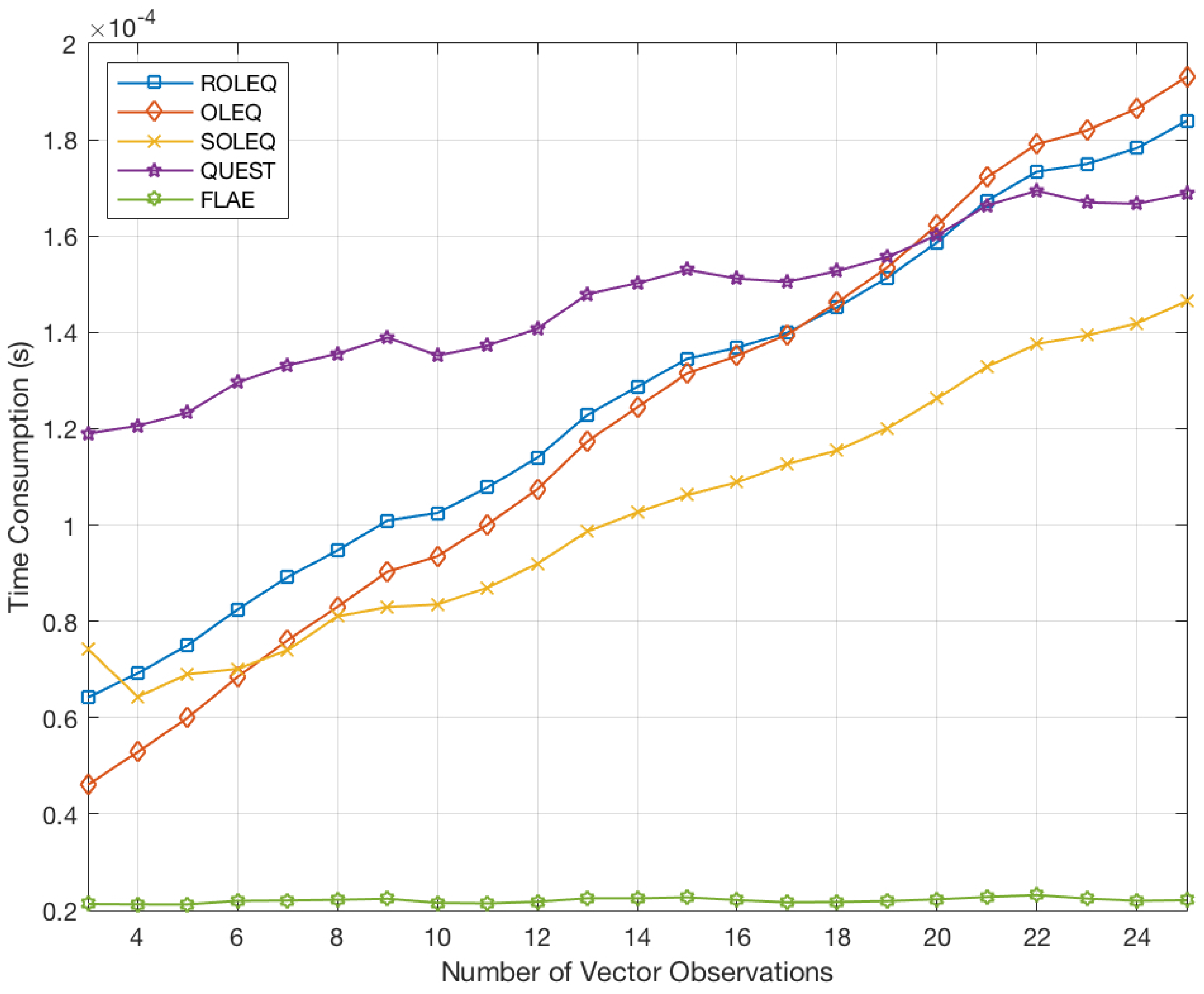
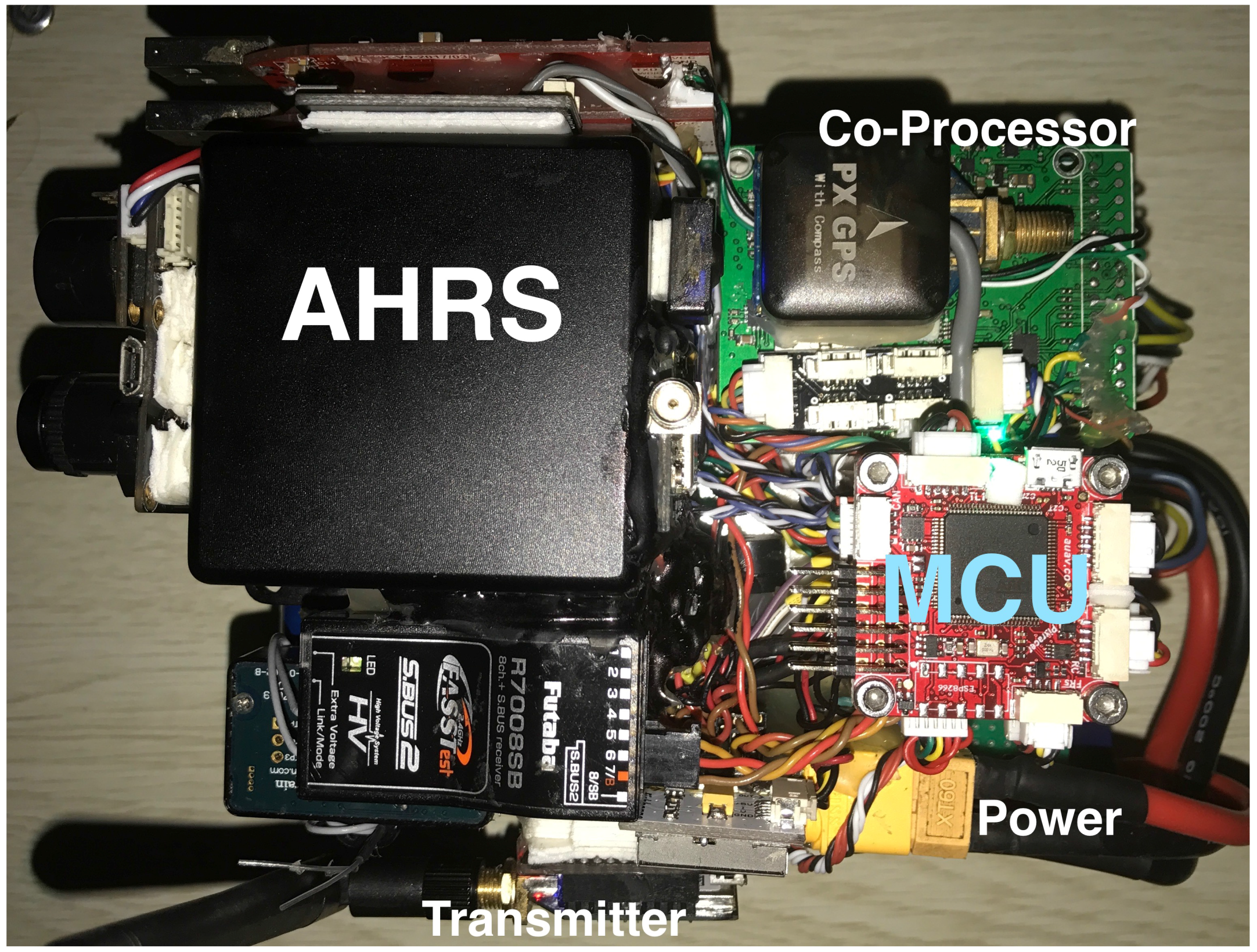
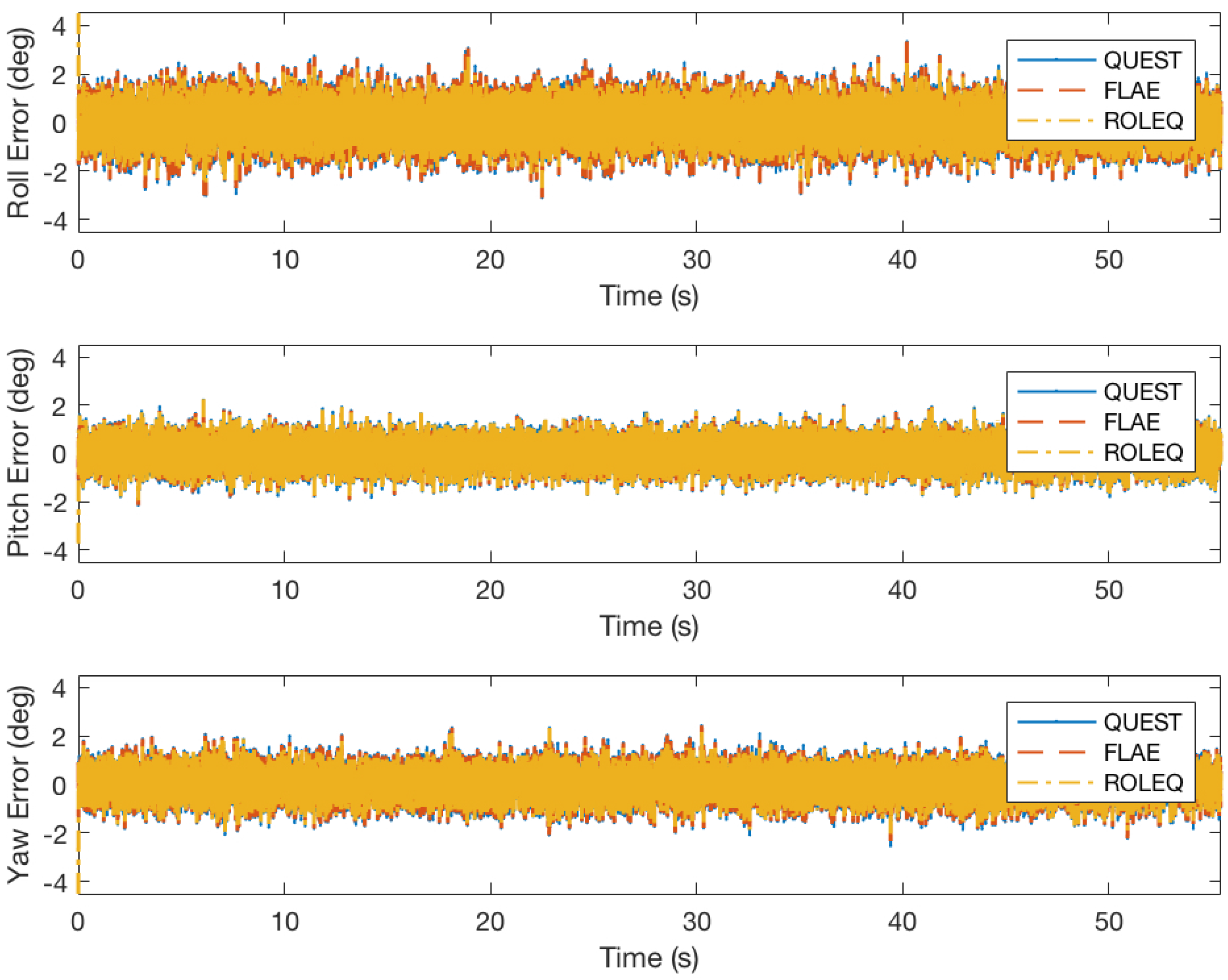
• Simulations and real experiments are carried out, which verify the accuracy, flexibility, robustness and time consumption of various algorithms for GNSS/AM attitude determination. Detailed comparisons with representative methods demonstrate the superiority of the proposed OLEQs.

This paper is structured as follows: Section 2 briefly introduces the GNSS-AM sensor system along with its functional and stochastic models formulated by vector pair matching. Section 3 contains the problem formulation and starts with the quaternion estimation from a single sensor observation. In Section 4, the two-vector attitude determination theory along with the n-vector theory are given accordingly. 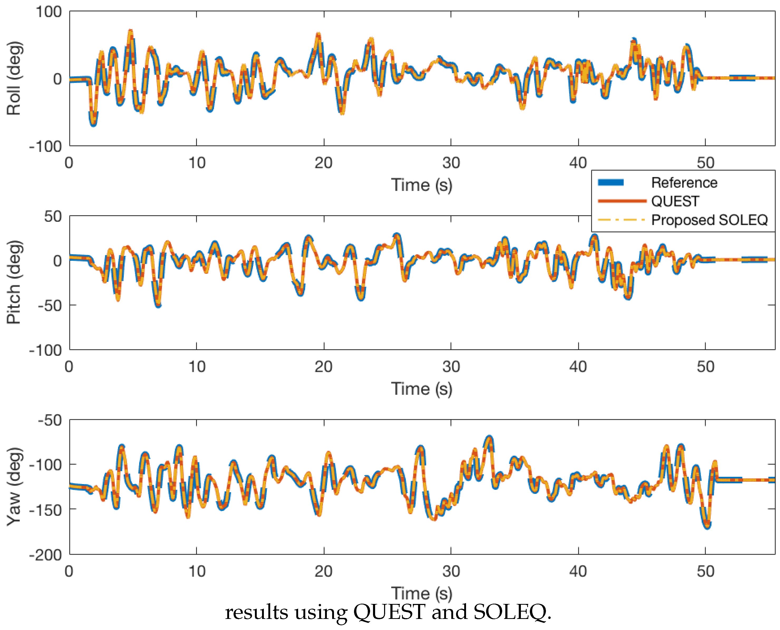Section 5 involves the numerical examples and the real field test where comparisons between the proposed SOLEQ and other representative methods are given. Finally, Section 6 consists of concluding remarks and future work.

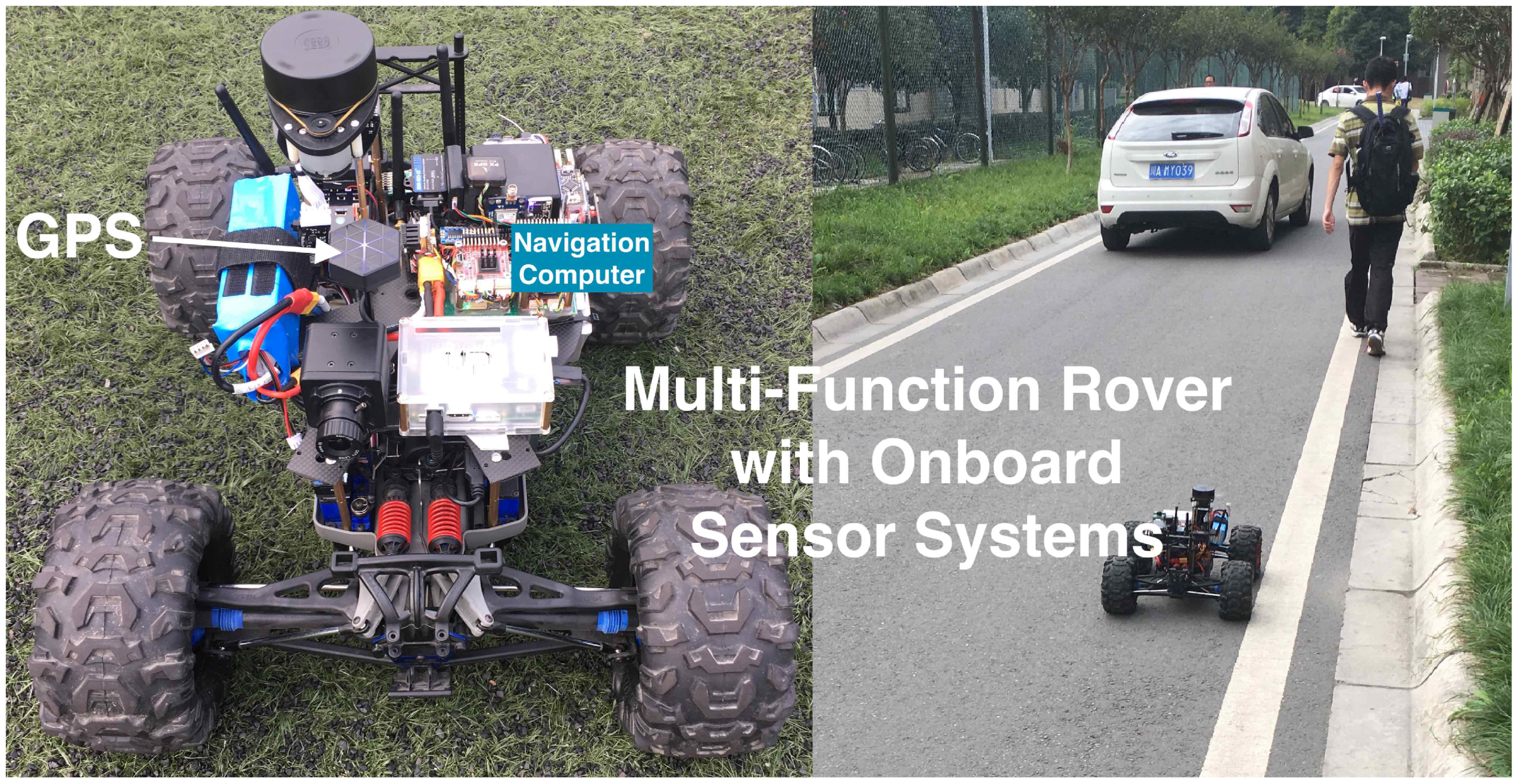
2. Fundamentals of the GNSS/AM System

For attitude determination, we require GNSS receivers and AM sensor arrays for low-cost and accurate solutions. First, considering the motion behaviours of land vehicles, a vector pair for GNSS velocity can be established as:

$${\mathbf{v}}_G^b={\mathbf{C}}_r^b{\mathbf{v}}_G^r+{\epsilon }_G^b$$

(1)

where $\mathbf{v}$ denotes velocity vector; the subscript G denotes the observation source ‘GNSS’; the symbols r and b represent the navigation frame (r-frame, North-East-Down (NED)) and body frame (b-frame, forward-right-down), respectively; the vector is transformed from the r-frame to the b-frame; ${\epsilon }_G^b$ is the Gaussian white noise with variance of ${\mathbf{R}}_G$. For the land-vehicle application, it should be pointed out that the velocities in the r-frame and the b-frame are respectively:

$${\mathbf{v}}^r={\mathbf{C}}_e^r{\mathbf{v}}^e,{\mathbf{v}}_G^b=\left[\begin{array}{c}\sqrt{{\left(v_x^e\right)}^2+{\left(v_y^e\right)}^2+{\left(v_z^e\right)}^2}\\ 0\\ 0\end{array}\right]$$

(2)

where e denotes an Earth-Centred-Earth-Fixed (ECEF) coordinate frame (e-frame), i.e., WGS-84; ${\mathbf{C}}_e^r$ denotes the transformation from the e-frame to the r-frame, which can be computed according to the GNSS position and Earth ellipsoid metrics in advance.

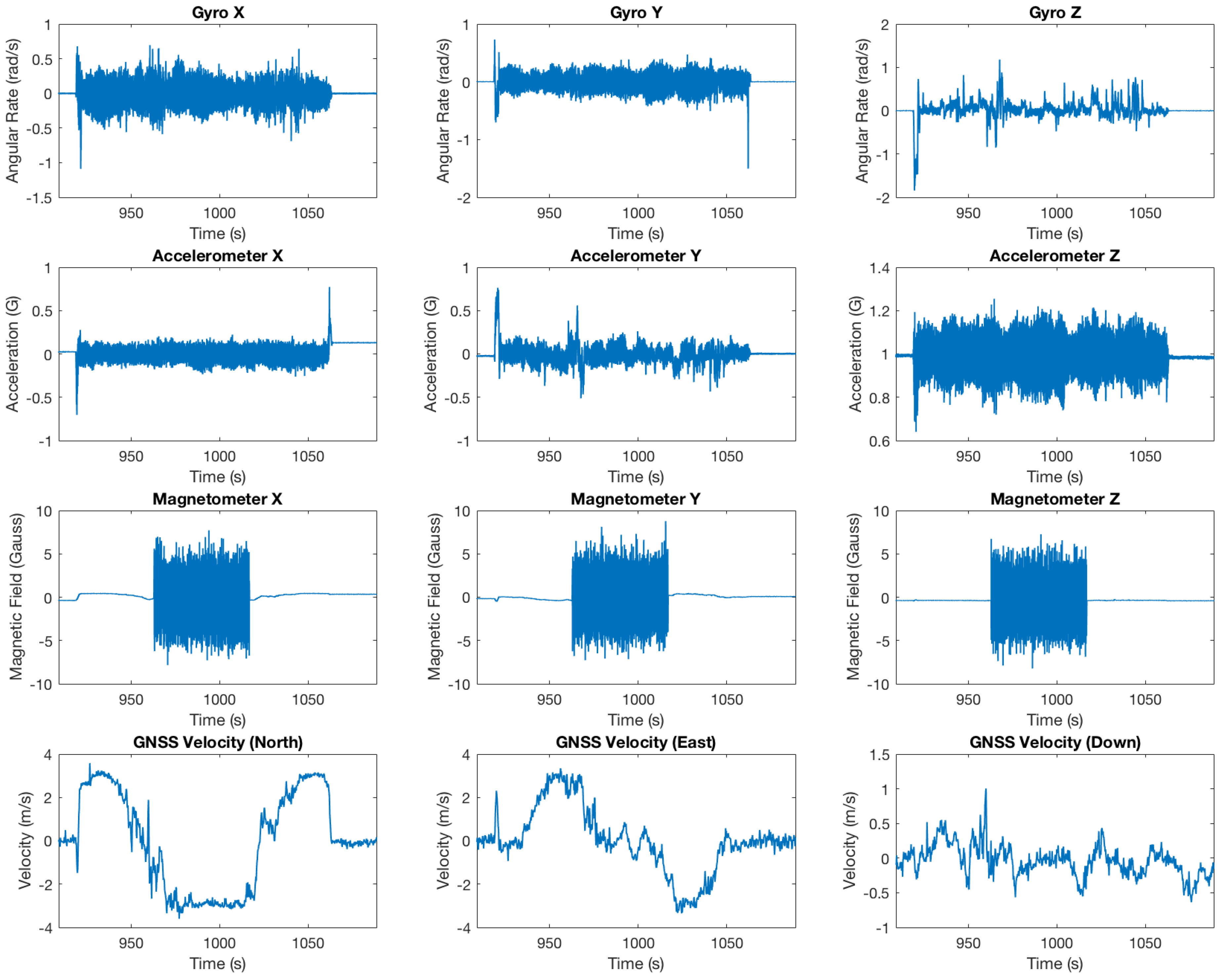
AM sensors consist of a three-axis MEMS accelerometer and three-axis magnetometer. The accelerometer gives the specific force measurement of a rigid body, and the magnetometer provides the users with the sensed local Earth geomagnetic field according to the IGRFmodel [35].

$$\begin{array}{cc}{\mathbf{z}}_A^{}={\mathbf{C}}_r^b({\mu }^r-{\mathbf{G}}^r)+{\mathbf{b}}_A+{\epsilon }_A,& {\epsilon }_A\sim \left(\mathbf{0},{\mathbf{R}}_A\right)\\ {\mathbf{z}}_M^{}={\mathbf{C}}_r^b{\mathbf{M}}^r+{\epsilon }_M,& {\epsilon }_M\sim \left(\mathbf{0},{\mathbf{R}}_M\right)\end{array}$$

(3)

where the subscripts A and M denote the accelerometer and magnetometer sources, respectively; $\mathbf{z}$ denotes the observed vector; $\mathbf{b}$ denotes the accelerometer bias; ${\mathbf{G}}^r={[0,0,-g]}^T$, where g is the gravity, is a function of the geo-location; the normalized Earth’s magnetic field reference vector ${\mathbf{M}}^r={[\cos \alpha ,0,-\sin \alpha ]}^T$, where $\alpha$ is the local dip angle; $\mu$ is the linear acceleration vector, which is usually treated as an external disturbance; $\epsilon$ is the Gaussian white noise with the variance of $\mathbf{R}$. For simplicity, two points need to be clarified that: (1) the bias term has been obtained and compensated for the accelerometer readings. (2) The linear acceleration $\mu$ is estimated by using GNSS velocity information with differentiation between two adjacent epochs. Then, the vectors and matrices for the system model in the b-frame and the r-frame can be merged into the following multi-vector pair equations:

$${\mathbf{D}}_i^b={\mathbf{C}}_r^b{\mathbf{D}}_i^r+{\epsilon }_i,i=1,2,3$$

(4)

where:

$$\left(\begin{array}{c}{\mathbf{D}}_1^b\\ {\mathbf{D}}_2^b\\ {\mathbf{D}}_3^b\end{array}\right)=\left(\begin{array}{c}\frac{{\mathbf{v}}_G^b}{∥{\mathbf{v}}_G^b∥}\\ \frac{{\mathbf{z}}_A}{∥{\mathbf{z}}_A∥}\\ \frac{{\mathbf{z}}_M}{∥{\mathbf{z}}_M∥}\end{array}\right),\left(\begin{array}{c}{\mathbf{D}}_1^r\\ {\mathbf{D}}_2^r\\ {\mathbf{D}}_3^r\end{array}\right)=\left(\begin{array}{c}\frac{{\mathbf{C}}_e^r{\mathbf{v}}_{}^e}{∥{\mathbf{C}}_e^r{\mathbf{v}}_{}^e∥}\\ \frac{{\mu }^r-{\mathbf{G}}^r}{∥{\mu }^r-{\mathbf{G}}^r∥}\\ \frac{{\mathbf{M}}^r}{∥{\mathbf{M}}^r∥}\end{array}\right),\left(\begin{array}{c}{\epsilon }_1\\ {\epsilon }_2\\ {\epsilon }_3\end{array}\right)=\left(\begin{array}{c}{\epsilon }_G\\ {\epsilon }_A\\ {\epsilon }_M\end{array}\right)$$

(5)

Neglecting the cross-correlations between sensors, the stochastic model of the system is:

$$\left(\begin{array}{c}{\epsilon }_G\\ {\epsilon }_A\\ {\epsilon }_M\end{array}\right)\sim (\mathbf{0},\mathbf{R}),\mathbf{R}=\left(\begin{array}{ccc}{\mathbf{R}}_G& & \\ & {\mathbf{R}}_A& \\ & & {\mathbf{R}}_M\end{array}\right)$$

(6)

3. Problem Formulation

The conventional Wahba’s problem aims to find the optimal attitude matrix from vector observation pairs in the sense of least-squares, such that:

$$L\left(\mathbf{C}\right)={\displaystyle \sum _{i=1}^n}{a}_i{∥{\mathbf{D}}_i^b-{\mathbf{CD}}_i^r∥}^2,n=2,3,\cdots$$

(7)

in which $\mathbf{C}$ denotes the optimal Direction Cosine Matrix (DCM); ${\mathbf{D}}_i^b={\left(D_{x,i}^b,D_{y,i}^b,D_{z,i}^b\right)}^{\top }$ and ${\mathbf{D}}_i^r={\left(D_{x,i}^r,D_{y,i}^r,D_{z,i}^r\right)}^{\top }$ are the i-th pair of normalized vector observations from the body frame b and the reference frame r, respectively; $a_i$ is the weight of the i-th sensor output, which is given by the standard deviations of the input vectors from ${\sigma }_1$ to ${\sigma }_n$:

$$a_i=\frac{1}{{\sigma }_i^2{\displaystyle \sum _{k=1}^n}\frac{1}{{\sigma }_k^2}}$$

(8)

provided that the variance information such as shown in Equation (6) is predetermined [22]. This ensures the biggest variance scalar with respect to the smallest weight. Wahba’s problem is solved via many representative methods [36]. Many of these algorithms solve the problem via eigenvalue decompositions analytically or numerically [28,29]. When there is only one pair of vector observations, Wahba’s solutions fail to obtain the optimal quaternion since there will be ambiguous quaternions corresponding to the maximum eigenvalue of one [37,38]. In our previous contribution [39], the continuous stable quaternion solution to an accelerometer-based attitude determination system is derived.

Quaternion from a Single Sensor Observation

Considering an attitude determination model from a pair of vector observations:

$${\mathbf{D}}^b=\mathbf{C}{\mathbf{D}}^r$$

(9)

this section deals with the attitude determination from a single pair of sensor observations. Note that the DCM is decomposed with quaternions $\mathbf{q}={(q_0,q_1,q_2,q_3)}^{\top }$ [39] via:

$$\mathbf{C}=({\mathbf{P}}_1\mathbf{q},{\mathbf{P}}_2\mathbf{q},{\mathbf{P}}_3\mathbf{q})$$

(10)

in which:

$${\mathbf{P}}_1=\left(\begin{array}{cccc}{q}_0& q_1& -q_2& -q_3\\ -q_3& q_2& q_1& -q_0\\ q_2& q_3& q_0& q_1\end{array}\right),{\mathbf{P}}_2=\left(\begin{array}{cccc}{q}_3& q_2& q_1& q_0\\ q_0& -q_1& q_2& -q_3\\ -q_1& -q_0& q_3& q_2\end{array}\right),{\mathbf{P}}_3=\left(\begin{array}{cccc}-q_2& q_3& -q_0& q_1\\ q_1& q_0& q_3& q_2\\ q_0& -q_1& -q_2& q_3\end{array}\right)$$

(11)

In this section, the theory is extended to an arbitrary sensor with a similar approach as in [39]. Inserting Equation (10) into Equation (9) yields:

$${\mathbf{D}}^b=(D_x^r{\mathbf{P}}_1+D_y^r{\mathbf{P}}_2+D_z^r{\mathbf{P}}_3)\mathbf{q}$$

(12)

It has been proven in [39] that:

$${\mathbf{P}}_1^{\top }={\mathbf{P}}_1^{†},{\mathbf{P}}_2^{\top }={\mathbf{P}}_2^{†},{\mathbf{P}}_3^{\top }={\mathbf{P}}_3^{†}$$

(13)

where † stands for the Moore–Penrose pseudo-inverse. In fact, another property can be deduced from the following theorem:

Theorem 1.

${\mathbf{P}}_1{\mathbf{P}}_2^{\top }+{\mathbf{P}}_2{\mathbf{P}}_1^{\top }={\mathbf{P}}_1{\mathbf{P}}_3^{\top }+{\mathbf{P}}_3{\mathbf{P}}_1^{\top }={\mathbf{P}}_2{\mathbf{P}}_3^{\top }+{\mathbf{P}}_3{\mathbf{P}}_2^{\top }={\mathbf{0}}_{3\times 3}$.

Proof. 

This can be proven via brute-force calculation:

$$\begin{array}{c}{\mathbf{P}}_1^{}{\mathbf{P}}_2^{\top }=\left(\begin{array}{ccc}0& -q_0^1+q_1^2+q_2^2-q_3^2& 2q_0{q}_1+2q_2{q}_3\\ q_0^1-q_1^2-q_2^2+q_3^2& 0& 2q_0{q}_2-2q_1{q}_3\\ -2q_0{q}_1-2q_2{q}_3& -2q_0{q}_2+2q_1{q}_3& 0\end{array}\right)\hfill \\ {\mathbf{P}}_2^{}{\mathbf{P}}_1^{\top }=\left(\begin{array}{ccc}0& q_0^1-q_1^2-q_2^2+q_3^2& -2q_0{q}_1-2q_2{q}_3\\ -q_0^1+q_1^2+q_2^2-q_3^2& 0& -2q_0{q}_2+2q_1{q}_3\\ 2q_0{q}_1+2q_2{q}_3& 2q_0{q}_2-2q_1{q}_3& 0\end{array}\right)\hfill \end{array}$$

(14a)

$$\begin{array}{c}{\mathbf{P}}_1^{}{\mathbf{P}}_3^{\top }=\left(\begin{array}{ccc}0& 2q_0{q}_1-2q_2{q}_3& q_0^1-q_1^2+q_2^2-q_3^2\\ -2q_0{q}_1+2q_2{q}_3& 0& -2q_1{q}_2-2q_0{q}_3\\ -q_0^1+q_1^2-q_2^2+q_3^2& 2q_1{q}_2+2q_0{q}_3& 0\end{array}\right)\hfill \\ {\mathbf{P}}_3^{}{\mathbf{P}}_1^{\top }=\left(\begin{array}{ccc}0& -2q_0{q}_1+2q_2{q}_3& -q_0^1+q_1^2-q_2^2+q_3^2\\ 2q_0{q}_1-2q_2{q}_3& 0& 2q_1{q}_2+2q_0{q}_3\\ q_0^1-q_1^2+q_2^2-q_3^2& -2q_1{q}_2-2q_0{q}_3& 0\end{array}\right)\hfill \end{array}$$

(14b)

$$\begin{array}{c}{\mathbf{P}}_2^{}{\mathbf{P}}_3^{\top }=\left(\begin{array}{ccc}0& 2q_0{q}_2+2q_1{q}_3& -2q_1{q}_2+2q_0{q}_3\\ -2q_0{q}_2-2q_1{q}_3& 0& q_0^1+q_1^2-q_2^2-q_3^2\\ 2q_1{q}_2-2q_0{q}_3& -q_0^1-q_1^2+q_2^2+q_3^2& 0\end{array}\right)\hfill \\ {\mathbf{P}}_3^{}{\mathbf{P}}_2^{\top }=\left(\begin{array}{ccc}0& -2q_0{q}_2-2q_1{q}_3& 2q_1{q}_2-2q_0{q}_3\\ 2q_0{q}_2+2q_1{q}_3& 0& -q_0^1-q_1^2+q_2^2+q_3^2\\ -2q_1{q}_2+2q_0{q}_3& q_0^1+q_1^2-q_2^2-q_3^2& 0\end{array}\right)\hfill \end{array}$$

(14c)

 ☐

Lemma 1.

Let $\mathbf{K}\left(\mathbf{q}\right)=(D_x^r{\mathbf{P}}_1+D_y^r{\mathbf{P}}_2+D_z^r{\mathbf{P}}_3)$, ${\mathbf{K}}^{\top }\left(\mathbf{q}\right)={\mathbf{K}}^{†}\left(\mathbf{q}\right)$.

Proof. 

We have:

$$\begin{array}{c}\mathbf{K}\left(\mathbf{q}\right){\mathbf{K}}^{\top }\left(\mathbf{q}\right)\hfill \\ =(D_x^r{\mathbf{P}}_1+D_y^r{\mathbf{P}}_2+D_z^r{\mathbf{P}}_3){(D_x^r{\mathbf{P}}_1+D_y^r{\mathbf{P}}_2+D_z^r{\mathbf{P}}_3)}^{\top }\hfill \\ ={\left(D_x^r\right)}^2{\mathbf{P}}_1{\mathbf{P}}_1^{\top }+{\left(D_y^r\right)}^2{\mathbf{P}}_2{\mathbf{P}}_2^{\top }+{\left(D_z^r\right)}^2{\mathbf{P}}_3{\mathbf{P}}_3^{\top }\hfill \\ +D_x^r{D}_y^r({\mathbf{P}}_1{\mathbf{P}}_2^{\top }+{\mathbf{P}}_2{\mathbf{P}}_1^{\top })+D_x^r{D}_z^r({\mathbf{P}}_1{\mathbf{P}}_3^{\top }+{\mathbf{P}}_3{\mathbf{P}}_1^{\top })+D_y^r{D}_z^r({\mathbf{P}}_2{\mathbf{P}}_3^{\top }+{\mathbf{P}}_3{\mathbf{P}}_2^{\top })\hfill \\ =\left[{\left(D_x^r\right)}^2+{\left(D_y^r\right)}^2+{\left(D_z^r\right)}^2\right]{\mathbf{I}}_{3\times 3}\hfill \\ ={\mathbf{I}}_{3\times 3}\hfill \end{array}$$

(15)

which gives Lemma 1. ☐

Hence, Equation (12) can be transformed into:

$${\mathbf{D}}^b=\mathbf{K}\left(\mathbf{q}\right)\mathbf{q}\Rightarrow {\mathbf{K}}^{†}\left(\mathbf{q}\right){\mathbf{D}}^b=\mathbf{q}\Rightarrow {\mathbf{K}}^{\top }\left(\mathbf{q}\right){\mathbf{D}}^b=\mathbf{q}$$

(16)

Since $\mathbf{K}\left(\mathbf{q}\right)$ is in the form of a quaternion, ${\mathbf{K}}^{\top }\left(\mathbf{q}\right){\mathbf{D}}^b$ can be expanded by:

$${\mathbf{K}}^{\top }\left(\mathbf{q}\right){\mathbf{D}}^b=D_x^r{\mathbf{P}}_1^{\top }{\mathbf{D}}^b+D_y^r{\mathbf{P}}_2^{\top }{\mathbf{D}}^b+D_z^r{\mathbf{P}}_3^{\top }{\mathbf{D}}^b$$

(17)

Furthermore, it can be obtained that:

$${\mathbf{P}}_1^{\top }{\mathbf{D}}^b=\left(\begin{array}{c}{D}_x^b{q}_0+D_z^b{q}_2-D_y^b{q}_3\hfill \\ D_x^b{q}_1+D_y^b{q}_2+D_z^b{q}_3\hfill \\ D_z^b{q}_0+D_y^b{q}_1-D_x^b{q}_2\hfill \\ -D_y^b{q}_0+D_z^b{q}_1-D_x^b{q}_3\hfill \end{array}\right)=\left(\begin{array}{cccc}{D}_x^b& 0& D_z^b& -D_y^b\\ 0& D_x^b& D_y^b& D_z^b\\ D_z^b& D_y^b& -D_x^b& 0\\ -D_y^b& D_z^b& 0& -D_x^b\end{array}\right)\mathbf{q}={\mathbf{M}}_1\mathbf{q}$$

(18a)

$${\mathbf{P}}_2^{\top }{\mathbf{D}}^b=\left(\begin{array}{c}{D}_y^b{q}_0-D_z^b{q}_1+D_x^b{q}_3\hfill \\ -D_z^b{q}_0-D_y^b{q}_1+D_x^b{q}_2\hfill \\ D_x^b{q}_1+D_y^b{q}_2+D_z^b{q}_3\hfill \\ D_x^b{q}_0+D_z^b{q}_2-D_y^b{q}_3\hfill \end{array}\right)=\left(\begin{array}{cccc}{D}_y^b& -D_z^b& 0& D_x^b\\ -D_z^b& -D_y^b& D_x^b& 0\\ 0& D_x^b& D_y^b& D_z^b\\ D_x^b& 0& D_z^b& -D_y^b\end{array}\right)\mathbf{q}={\mathbf{M}}_2\mathbf{q}$$

(18b)

$${\mathbf{P}}_3^{\top }{\mathbf{D}}^b=\left(\begin{array}{c}{D}_z^b{q}_0+D_y^b{q}_1-D_x^b{q}_2\hfill \\ D_y^b{q}_0-D_z^b{q}_1+D_x^b{q}_3\hfill \\ -D_x^b{q}_0-D_z^b{q}_2+D_y^b{q}_3\hfill \\ D_x^b{q}_1+D_y^b{q}_2+D_z^b{q}_3\hfill \end{array}\right)=\left(\begin{array}{cccc}{D}_z^b& D_y^b& -D_x^b& 0\\ D_y^b& -D_z^b& 0& D_x^b\\ -D_x^b& 0& -D_z^b& D_y^b\\ 0& D_x^b& D_y^b& D_z^b\end{array}\right)\mathbf{q}={\mathbf{M}}_3\mathbf{q}$$

(18c)

Then, we have:

$${\mathbf{K}}^{\top }\left(\mathbf{q}\right){\mathbf{D}}^b=D_x^r{\mathbf{M}}_1\mathbf{q}+D_y^r{\mathbf{M}}_2\mathbf{q}+D_z^r{\mathbf{M}}_3\mathbf{q}=\mathbf{Wq}$$

(19)

where $\mathbf{W}$ is given by:

$$\mathbf{W}=D_x^r{\mathbf{M}}_1+D_y^r{\mathbf{M}}_2+D_z^r{\mathbf{M}}_3$$

(20)

Therefore, the attitude determination problem is shifted to:

$$\mathbf{Wq}=\mathbf{q}$$

(21)

Theorem 2.

For any normalized vector observation pair $\left\{{\mathbf{D}}^r,{\mathbf{D}}^b\right\}$, ${\mathbf{W}}^2=\mathbf{I}$, where $\mathbf{I}$ is the four-dimensional identity matrix.

Proof. 

The characteristic polynomial of $\mathbf{W}$ is given by:

$$p\left(\lambda \right)={(\lambda -1)}^2{(\lambda +1)}^2$$

(22)

Then, with the Cayley–Hamilton theorem, we substitute $\mathbf{W}$ for its eigenvalues and obtain:

$${\left({\mathbf{W}}^2-\mathbf{I}\right)}^2=\mathbf{0}$$

(23)

and as ${\mathbf{W}}^2-\mathbf{I}$ is real symmetric, it should be $\mathbf{0}$, which completes the proof. ☐

According to our previous contribution [39], Equation (21) can be treated as an iterative dynamical system:

$$\mathbf{q}\left(n\right)=\mathbf{Wq}(n-1)$$

(24)

where $\mathbf{q}\left(n\right)$ denotes the quaternion for the n-th iteration. Furthermore, as has been proven, the discrete-time system can be converted to a corresponding continuous system. If ${\mathbf{W}}^2=\mathbf{I}$, the stable solution to the continuous-time system is calculated as:

$$\mathbf{q}=\frac{\mathbf{W}+\mathbf{I}}{2}{\mathbf{q}}_{rand}$$

(25)

where ${\mathbf{q}}_{rand}$ denotes a randomly-chosen unit quaternion. This provides us with a new approach to obtaining the measurement quaternion from a single strapdown sensor.

4. Optimal Linear Estimator of the Quaternion

With Equation (9), it is possible to list all the single rotation equations together as follows:

$$\left\{\begin{array}{c}{\mathbf{D}}_1^b={\mathbf{CD}}_1^r\\ {\mathbf{D}}_2^b={\mathbf{CD}}_2^r\\ ⋮\\ {\mathbf{D}}_n^b={\mathbf{CD}}_n^r\end{array}\right.\Rightarrow \left\{\begin{array}{c}\sqrt{a_1}{\mathbf{D}}_1^b=\sqrt{a_1}{\mathbf{CD}}_1^r\\ \sqrt{a_2}{\mathbf{D}}_2^b=\sqrt{a_2}{\mathbf{CD}}_2^r\\ ⋮\\ \sqrt{a_n}{\mathbf{D}}_n^b=\sqrt{a_n}{\mathbf{CD}}_n^r\end{array}\right.$$

(26)

which can in turn be converted to:

$$\left\{\begin{array}{c}\sqrt{a_1}\mathbf{q}=\sqrt{a_1}{\mathbf{W}}_1\mathbf{q}\\ \sqrt{a_2}\mathbf{q}=\sqrt{a_2}{\mathbf{W}}_2\mathbf{q}\\ ⋮\\ \sqrt{a_n}\mathbf{q}=\sqrt{a_n}{\mathbf{W}}_n\mathbf{q}\end{array}\right.$$

(27)

This system is rewritten as:

$$\left(\begin{array}{c}\sqrt{a_1}\mathbf{I}\\ \sqrt{a_2}\mathbf{I}\\ ⋮\\ \sqrt{a_n}\mathbf{I}\end{array}\right)\mathbf{q}=\left(\begin{array}{c}\sqrt{a_1}{\mathbf{W}}_1\\ \sqrt{a_2}{\mathbf{W}}_2\\ ⋮\\ \sqrt{a_n}{\mathbf{W}}_n\end{array}\right)\mathbf{q}$$

(28)

Noticing that:

$$\left(\sqrt{a_1}\mathbf{I},\sqrt{a_2}\mathbf{I},\cdots ,\sqrt{a_n}\mathbf{I}\right)\left(\begin{array}{c}\sqrt{a_1}\mathbf{I}\\ \sqrt{a_2}\mathbf{I}\\ ⋮\\ \sqrt{a_n}\mathbf{I}\end{array}\right)=\left({\displaystyle \sum _{i=1}^n}{a}_i\right)\mathbf{I}=\mathbf{I}$$

(29)

hence the pre-multiplication leads to:

$$\mathbf{q}=\left({\displaystyle \sum _{i=1}^n}{a}_i{\mathbf{W}}_i\right)\mathbf{q}$$

(30)

It should be then noted that Equation (28) is free of noises. In this case, the maximum eigenvalue of ${\displaystyle \sum _{i=1}^n}{a}_i{\mathbf{W}}_i$ in engineering practice is very close to the noise-free theoretical result of one. Corresponding to Equation (24), based on Brouwer’s fixed-point theorem, it is possible to recursively obtain the normalized optimal quaternion by rotating a randomly given initial quaternion over and over again to infinity. This is something similar to the power method of the numerical eigenvalue factorization, but can be accelerated with geometric series-like iterations as follows:

$$\begin{array}{c}\mathcal{R}=\left({\displaystyle \sum _{i=1}^n}{a}_i{\mathbf{W}}_i\right)\hfill \\ {\mathcal{R}}^2=\mathcal{R}·\mathcal{R}\hfill \\ ⋮\hfill \\ {\mathcal{R}}^{2^j}={\mathcal{R}}^{2^{j-1}}·{\mathcal{R}}^{2^{j-1}}\hfill \end{array}$$

(31)

where $\mathcal{R}$ denotes the rotation operator over the Hamilton space $\mathbb{H}$. In fact, the above iterations can hardly be achieved when the maximum eigenvalue approaches one. The reason is that at this time, the power ${\mathcal{R}}^2$ approaches $\mathbf{I}$, as well. A more robust way is shown to solve this problem. Considering both sides of Equation (28), we find out that the right side is in fact the mixture of solutions to single vector observation pairs. As mentioned in Equation (25), a stable and continuous solution to each single equation can be done by pre-multiplying $\frac{1}{2}({\mathbf{W}}_i+\mathbf{I})$. Substituting $\frac{1}{2}({\mathbf{W}}_i+\mathbf{I})$ for ${\mathbf{W}}_i$, i.e.,

$$\left(\begin{array}{c}\sqrt{a_1}\mathbf{I}\\ \sqrt{a_2}\mathbf{I}\\ ⋮\\ \sqrt{a_n}\mathbf{I}\end{array}\right)\mathbf{q}=\left[\begin{array}{c}\frac{1}{2}\sqrt{a_1}({\mathbf{W}}_1+\mathbf{I})\\ \frac{1}{2}\sqrt{a_2}({\mathbf{W}}_2+\mathbf{I})\\ ⋮\\ \frac{1}{2}\sqrt{a_n}({\mathbf{W}}_n+\mathbf{I})\end{array}\right]\mathbf{q}$$

(32)

the quaternion evolutes are from the mixture of the single optimal solution. Here, the rotation operator is revised as:

$$\mathcal{R}={\displaystyle \sum _{i=1}^n}\frac{1}{2}{a}_i({\mathbf{W}}_i+\mathbf{I})=\frac{1}{2}\left(\mathbf{I}+{\displaystyle \sum _{i=1}^n}{a}_i{\mathbf{W}}_i\right)$$

(33)

This equals the least-square of the set of pre-computed single rotated quaternions, which is definitely faster and more robust than rotation from a randomly given initial quaternion.

The covariance of the calculated optimal quaternion is equal to that of QUEST under the condition of least-square optimality:

$$\begin{array}{c}{\Sigma }_{\mathbf{Q},\mathrm{OLEQ}}=\frac{1}{4{\displaystyle \sum _{i=1}^n}\frac{1}{{\sigma }_i^2}}\left(\mathbf{I}-{\displaystyle \sum _{i=1}^n}{\mathbf{D}}^b{\left\{{\mathbf{D}}^b\right\}}^{\top }\right)\hfill \\ {\Sigma }_{\mathbf{q},\mathrm{OLEQ}}=\left[{\mathbf{q}}_{\mathrm{OLEQ}}\right]\left(\begin{array}{cc}0& {\mathbf{0}}_{1\times 3}\\ {\mathbf{0}}_{3\times 1}& {\Sigma }_{\mathbf{Q},\mathrm{OLEQ}}\end{array}\right){\left[{\mathbf{q}}_{\mathrm{OLEQ}}\right]}^{\top }\hfill \end{array}$$

(34)

where $\mathbf{Q}={(q_1,q_2,q_3)}^{\top }$ is the vector part of the quaternion. $\left[\mathbf{q}\right]$ defines the following matrix:

$$\left[\mathbf{q}\right]=\left(\begin{array}{cccc}{q}_3& -q_2& q_1& q_0\\ q_2& q_3& -q_0& q_1\\ -q_1& q_0& q_3& q_2\\ -q_0& -q_1& -q_2& q_3\end{array}\right)$$

(35)

4.1. Variant 1: Recursive-OLEQ

We have seen from the above formulations that for each epoch, the vector observations are batch processed thoroughly. When used in aerospace electronic systems, the measured vector observation pairs in neighbouring time epochs are usually continuous since they are always smoothed by the sum filters and Low-Pass Filters (LPF). Therefore, with this consideration, the attitude quaternion can be propagated from the last estimated one using the rotation operator described before. In this way, the quaternions are recursively computed with much fewer computations, and the accuracy is maintained. Furthermore, for highly-reliable attitude determination systems, high-precision gyroscopes are usually employed. This provides us with a second-stage acceleration scheme, inspired by the conventional recursive algorithms like filter QUEST, REQUEST, etc. [40], by which we may first rotate the estimated quaternion in the last time epoch with the zero-order angular transition matrix by:

$${\mathbf{q}}_k={\mathbf{\Phi }}_{k,k-1}{\mathbf{q}}_{k-1}$$

(36)

where:

$${\mathbf{\Phi }}_{k,k-1}=\mathbf{I}+\frac{\Delta t}{2}\left[\Omega \times \right]$$

(37)

in which $\Delta t$ is the sampling time and $\left[\Omega \times \right]$ composed by the angular rate from the gyroscope, which is detailed in many classical literature works [41]. After this, even a single rotation by $\mathcal{R}$ would then be very accurate. The one-step covariance matrix of the obtained quaternion is calculated by:

$${\Sigma }_{{\mathbf{q}}_k,\mathrm{ROLEQ}}=\mathcal{R}{\mathbf{\Phi }}_{k,k-1}{\Sigma }_{{\mathbf{q}}_{k-1},\mathrm{ROLEQ}}{\mathbf{\Phi }}_{k,k-1}^{\top }{\mathcal{R}}^{\top }$$

(38)

4.2. Variant 2: SOLEQ

4.2.1. Two-Vector Case

When there are two pairs of vector observations, regardless of the weights of the respective sensors, it is natural that the attitude quaternion may be computed via:

$$\mathbf{q}=\frac{1}{4}\left({\mathbf{W}}_1+\mathbf{I}\right)\left({\mathbf{W}}_2+\mathbf{I}\right){\mathbf{q}}_{rand}$$

(39)

where ${\mathbf{W}}_1$ and ${\mathbf{W}}_2$ are for the first and second sensors. Equation (25) is reasonable since we have:

$${\left[\frac{1}{2}\left(\mathbf{W}+\mathbf{I}\right)\right]}^2=\frac{1}{4}\left({\mathbf{W}}^2+2\mathbf{W}+\mathbf{I}\right)=\frac{1}{4}\left(2\mathbf{W}+2\mathbf{I}\right)=\frac{1}{2}\left(\mathbf{W}+\mathbf{I}\right)$$

(40)

However, for the two-vector case, one can write:

$$\begin{array}{c}{\left[\frac{1}{4}\left({\mathbf{W}}_1+\mathbf{I}\right)\left({\mathbf{W}}_2+\mathbf{I}\right)\right]}^2={\left[\frac{1}{4}\left({\mathbf{W}}_1{\mathbf{W}}_2+{\mathbf{W}}_1+{\mathbf{W}}_2+\mathbf{I}\right)\right]}^2\ne \frac{1}{4}\left({\mathbf{W}}_1+\mathbf{I}\right)\left({\mathbf{W}}_2+\mathbf{I}\right)\hfill \end{array}$$

(41)

This reflects that the accurate quaternion can be recursively computed with:

$$\left\{\begin{array}{c}{\mathbf{q}}_k=\frac{1}{4}\left({\mathbf{W}}_1+\mathbf{I}\right)\left({\mathbf{W}}_2+\mathbf{I}\right){\mathbf{q}}_{k-1}\\ {\mathbf{q}}_k=\frac{{\mathbf{q}}_k}{∥{\mathbf{q}}_k∥}\end{array}\right.$$

(42)

which exits when the Euler distance $∥{\mathbf{q}}_k-{\mathbf{q}}_{k-1}∥$ is less than one predetermined threshold $\eta$. Note that the above initialization procedure is equivalent to the following process:

$$\left\{\begin{array}{c}{\mathbf{q}}^j={\left[\frac{1}{4}\left({\mathbf{W}}_1+\mathbf{I}\right)\left({\mathbf{W}}_2+\mathbf{I}\right)\right]}^j{\mathbf{q}}_{rand}\\ {\mathbf{q}}^j=\frac{{\mathbf{q}}^j}{∥{\mathbf{q}}^j∥}\end{array}\right.$$

(43)

where ${\mathbf{q}}_{rand}$ is a randomly chosen quaternion; j is chosen to make sure $∥{\mathbf{q}}^j-{\mathbf{q}}^{j-1}∥<\eta$. Let us define the following transformation operators:

$$\mathcal{A}=\frac{1}{4}\left({\mathbf{W}}_1+\mathbf{I}\right)\left({\mathbf{W}}_2+\mathbf{I}\right)$$

(44a)

$$\mathcal{B}={\mathcal{A}}^{\top }=\frac{1}{4}\left({\mathbf{W}}_2+\mathbf{I}\right)\left({\mathbf{W}}_1+\mathbf{I}\right)$$

(44b)

Theorem 3.

For the two-vector attitude determination case, the steady-state evolution in Equation (43) is not affected by the transformation operators’ order, such that:

$$\left\{\begin{array}{c}{\mathbf{q}}^j={\mathcal{A}}^j{\mathbf{q}}_{rand}\\ {\mathbf{q}}^j=\frac{{\mathbf{q}}^j}{∥{\mathbf{q}}^j∥}\end{array}\right.\iff \left\{\begin{array}{c}{\mathbf{q}}^j={\mathcal{B}}^j{\mathbf{q}}_{rand}\\ {\mathbf{q}}^j=\frac{{\mathbf{q}}^j}{∥{\mathbf{q}}^j∥}\end{array}\right.,j\to +\infty$$

(45)

Proof. 

The integrated transformation can be computed by:

$$\begin{array}{c}\mathcal{AB}=\frac{1}{16}\left({\mathbf{W}}_1+\mathbf{I}\right){\left({\mathbf{W}}_2+\mathbf{I}\right)}^2\left({\mathbf{W}}_1+\mathbf{I}\right)=\frac{1}{8}\left({\mathbf{W}}_1+\mathbf{I}\right)\left({\mathbf{W}}_2+\mathbf{I}\right)\left({\mathbf{W}}_1+\mathbf{I}\right)\hfill \\ =\frac{1}{2}\mathcal{A}\left({\mathbf{W}}_1+\mathbf{I}\right)=\frac{1}{2}\left({\mathbf{W}}_1+\mathbf{I}\right)\mathcal{B}\hfill \end{array}$$

(46)

and accordingly

$$\mathcal{B}\mathcal{A}=\frac{1}{2}\mathcal{B}\left({\mathbf{W}}_2+\mathbf{I}\right)=\frac{1}{2}\left({\mathbf{W}}_2+\mathbf{I}\right)\mathcal{A}$$

(47)

These generate:

$$\begin{array}{c}\mathcal{ABA}=\frac{1}{2}\left({\mathbf{W}}_1+\mathbf{I}\right)\mathcal{BA}=\frac{1}{4}\left({\mathbf{W}}_1+\mathbf{I}\right)\left({\mathbf{W}}_2+\mathbf{I}\right)\mathcal{A}={\mathcal{A}}^2\hfill \end{array}$$

(48)

and:

$$\mathcal{A}\mathcal{B}\mathcal{A}\mathcal{B}={\mathcal{A}}^2\mathcal{B}=\mathcal{A}\left(\mathcal{A}\mathcal{B}\right)=\frac{1}{2}{\mathcal{A}}^2\left({\mathbf{W}}_1+\mathbf{I}\right)$$

(49)

Finally, we have:

$${\left(\mathcal{A}\mathcal{B}\right)}^j=\frac{1}{2}{\mathcal{A}}^j\left({\mathbf{W}}_1+\mathbf{I}\right)=\frac{1}{2}\left({\mathbf{W}}_1+\mathbf{I}\right){\mathcal{B}}^j$$

(50)

This proves that the mixed steady-state transformation ${\left(\mathcal{A}\mathcal{B}\right)}^j$ can be achieved by independent transformations from $\mathcal{A}$ or $\mathcal{B}$, which completes the proof. ☐

Following this theorem, the problem is to compute the power ${\mathcal{A}}^j$. In fact, $\mathcal{A}$ is formed with $\frac{1}{2}\left({\mathbf{W}}_1+\mathbf{I}\right)$ and $\frac{1}{2}\left({\mathbf{W}}_2+\mathbf{I}\right)$. Their respective eigenvalue decompositions can be given by:

$$\left\{\begin{array}{c}\frac{1}{2}\left({\mathbf{W}}_1+\mathbf{I}\right)={\mathbf{V}}_1{\mathbf{S}}_1{\mathbf{V}}_1^{-1}={\mathbf{V}}_1{\mathbf{S}}_1{\mathbf{V}}_1^{\top }\\ \frac{1}{2}\left({\mathbf{W}}_2+\mathbf{I}\right)={\mathbf{V}}_2{\mathbf{S}}_2{\mathbf{V}}_2^{-1}={\mathbf{V}}_2{\mathbf{S}}_2{\mathbf{V}}_2^{\top }\end{array}\right.$$

(51)

where $\mathbf{V}$ and $\mathbf{D}$ are constituted by eigenvectors and eigenvalues respectively as $\left({\mathbf{W}}_i+\mathbf{I}\right)$ is real symmetric [42]. Since ${\mathbf{W}}_1$ and ${\mathbf{W}}_2$ are in the same form, the eigenvalue matrices are equal to each other, i.e.,

$${\mathbf{S}}_1={\mathbf{S}}_2=\mathbf{S}$$

(52)

Then, $\mathcal{A}$ can be rewritten as:

$$\mathcal{A}={\mathbf{V}}_1\mathbf{S}{\mathbf{V}}_1^{\top }{\mathbf{V}}_2\mathbf{S}{\mathbf{V}}_2^{\top }$$

(53)

Identically, we have:

$$\mathcal{B}={\mathbf{V}}_2\mathbf{S}{\mathbf{V}}_2^{\top }{\mathbf{V}}_1\mathbf{S}{\mathbf{V}}_1^{\top }$$

(54)

Combining Equations (53) and (54), it is obtained that:

$$\mathcal{A}\mathcal{B}={\mathbf{V}}_1\mathbf{S}{\mathbf{V}}_1^{\top }{\mathbf{V}}_2\mathbf{S}{\mathbf{V}}_2^{\top }{\mathbf{V}}_2\mathbf{S}{\mathbf{V}}_2^{\top }{\mathbf{V}}_1\mathbf{S}{\mathbf{V}}_1^{\top }$$

(55)

Note that:

$${\mathbf{V}}_1{\mathbf{V}}_1^{\top }={\mathbf{V}}_1^{\top }{\mathbf{V}}_1^{}={\mathbf{V}}_2{\mathbf{V}}_2^{\top }={\mathbf{V}}_2^{\top }{\mathbf{V}}_2^{}=\mathbf{I}$$

(56)

Equation (55) is simplified as:

$$\mathcal{A}\mathcal{B}={\mathbf{V}}_1\mathbf{S}{\mathbf{V}}_1^{\top }{\mathbf{V}}_2\mathbf{S}\mathbf{S}{\mathbf{V}}_2^{\top }{\mathbf{V}}_1\mathbf{S}{\mathbf{V}}_1^{\top }$$

(57)

Here, we define:

$$\mathbf{U}={\mathbf{SV}}_1^{\top }{\mathbf{V}}_2{\mathbf{S}}^2{\mathbf{V}}_2^{\top }{\mathbf{V}}_1\mathbf{S}$$

(58)

Actually, it can be decomposed by:

$$\begin{array}{c}\mathbf{U}=\mathbf{H}{\mathbf{H}}^{\top }\\ \mathbf{H}={\mathbf{SV}}_1^{\top }{\mathbf{V}}_2\mathbf{S}\end{array}$$

(59)

An interesting fact is that the eigenvalue matrix $\mathbf{S}$ can be analytically calculated and is given by:

$$\mathbf{S}=diag(0,0,1,1)$$

(60)

where $diag(·)$ represents the diagonal matrix. This further yields $\mathbf{H}$ to be a matrix with the form of:

$$\mathbf{H}=\left(\begin{array}{cccc}0& 0& 0& 0\\ 0& 0& 0& 0\\ 0& 0& h_1& h_2\\ 0& 0& h_3& h_4\end{array}\right)$$

(61)

Then, $\mathbf{U}$ is computed by:

$$\begin{array}{c}\mathbf{U}=\mathbf{H}{\mathbf{H}}^{\top }=\left(\begin{array}{cccc}0& 0& 0& 0\\ 0& 0& 0& 0\\ 0& 0& u_1& u_2\\ 0& 0& u_3& u_4\end{array}\right)=\left(\begin{array}{cccc}0& 0& 0& 0\\ 0& 0& 0& 0\\ 0& 0& h_1^2+h_2^2& h_1^{}{h}_3^{}+h_2^{}{h}_4^{}\\ 0& 0& h_1^{}{h}_3^{}+h_2^{}{h}_4^{}& h_3^2+h_4^2\end{array}\right)\hfill \end{array}$$

(62)

where $u_2=u_3$. Using this, we have:

$${\left(\mathcal{A}\mathcal{B}\right)}^j={\mathbf{V}}_1{\mathbf{UV}}_1^{\top }{\mathbf{V}}_1{\mathbf{UV}}_1^{\top }\cdots {\mathbf{V}}_1{\mathbf{UV}}_1^{\top }={\mathbf{V}}_1{\mathbf{U}}^j{\mathbf{V}}_1^{\top }$$

(63)

$\mathbf{U}$ can be decomposed with eigenvalue decomposition as well, such that:

$$\mathbf{U}={\mathbf{V}}_{\mathbf{U}}{\mathbf{S}}_{\mathbf{U}}{\mathbf{V}}_{\mathbf{U}}^T$$

(64)

which can be analytically given by:

$$\begin{array}{c}{\mathbf{S}}_{\mathbf{U}}=diag\left(0,0,-\frac{1}{2}\sqrt{\Delta }+\frac{u_1^{}+u_4^{}}{2},+\frac{1}{2}\sqrt{\Delta }+\frac{u_1^{}+u_4^{}}{2}\right)\hfill \\ {\mathbf{V}}_{\mathbf{U}}=\left(\begin{array}{cccc}1& 0& 0& 0\\ 0& 1& 0& 0\\ 0& 0& \frac{-u_1+u_4+\sqrt{\Delta }}{2u_2}& \frac{u_1-u_4+\sqrt{\Delta }}{2u_2}\\ 0& 0& 1& 1\end{array}\right)\hfill \end{array}$$

(65)

with:

$$\Delta =u_1^2-2u_1^{}{u}_4^{}+4u_2^2+u_4^2$$

(66)

Letting:

$$\begin{array}{c}{\lambda }_{\mathbf{U},1}=-\frac{1}{2}\sqrt{\Delta }+\frac{u_1^{}+u_4^{}}{2}\\ {\lambda }_{\mathbf{U},2}=+\frac{1}{2}\sqrt{\Delta }+\frac{u_1^{}+u_4^{}}{2}\end{array}$$

(67)

${\mathbf{U}}^j$ is finally computed by:

$${\mathbf{U}}^j={\mathbf{V}}_{\mathbf{U}}{\mathbf{S}}^j{\mathbf{V}}_{\mathbf{U}}^T={\mathbf{V}}_{\mathbf{U}}diag(0,0,{\lambda }_{\mathbf{U},1}^j,{\lambda }_{\mathbf{U},2}^j){\mathbf{V}}_{\mathbf{U}}^T$$

(68)

Therefore:

$${\left(\mathcal{A}\mathcal{B}\right)}^j={\mathbf{V}}_1{\mathbf{U}}^j{\mathbf{V}}_1^{\top }={\mathbf{V}}_1{\mathbf{V}}_{\mathbf{U}}diag(0,0,{\lambda }_{\mathbf{U},1}^j,{\lambda }_{\mathbf{U},2}^j){\mathbf{V}}_{\mathbf{U}}^{\top }{\mathbf{V}}_1^{\top }$$

(69)

The required computation of ${\mathbf{V}}_i$ is computed as follows:

$$\frac{1}{2}\left({\mathbf{W}}_i+\mathbf{I}\right)={\tilde{\mathbf{V}}}_i{\mathbf{S}\tilde{\mathbf{V}}}_i^{-1}$$

(70)

where ${\tilde{\mathbf{V}}}_i(x,y)$ stands for the element of ${\tilde{\mathbf{V}}}_i$ in the x-th row and the y-th column, the details of which are given by Equation (71):

$$\begin{array}{c}{\tilde{\mathbf{V}}}_i(1,1)=+\frac{1}{V_i}(D_{x,i}^b-D_{x,i}^r)(D_{z,i}^b-D_{z,i}^r)\hfill \\ {\tilde{\mathbf{V}}}_i(1,2)=-\frac{1}{V_i}(D_{x,i}^b-D_{x,i}^r)(D_{y,i}^b-D_{y,i}^r)\hfill \\ {\tilde{\mathbf{V}}}_i(1,3)=+\frac{1}{V_i}(D_{x,i}^b+D_{x,i}^r)(D_{z,i}^b+D_{z,i}^r)\hfill \\ {\tilde{\mathbf{V}}}_i(1,4)=-\frac{1}{V_i}(D_{x,i}^b+D_{x,i}^r)(D_{y,i}^b+D_{y,i}^r)\hfill \end{array}$$

(71a)

$$\begin{array}{c}{\tilde{\mathbf{V}}}_i(2,1)=+\frac{1}{V_i}(D_{x,i}^b-D_{x,i}^r)(D_{y,i}^b+D_{y,i}^r)\hfill \\ {\tilde{\mathbf{V}}}_i(2,2)=+\frac{1}{V_i}(D_{x,i}^b-D_{x,i}^r)(D_{z,i}^b+D_{z,i}^r)\hfill \\ {\tilde{\mathbf{V}}}_i(2,3)=+\frac{1}{V_i}(D_{x,i}^b+D_{x,i}^r)(D_{y,i}^b-D_{y,i}^r)\hfill \\ {\tilde{\mathbf{V}}}_i(2,4)=+\frac{1}{V_i}(D_{x,i}^b+D_{x,i}^r)(D_{z,i}^b-D_{z,i}^r)\hfill \end{array}$$

(71b)

$$\begin{array}{c}\begin{array}{cccc}{\tilde{\mathbf{V}}}_i(3,1)=1& {\tilde{\mathbf{V}}}_i(3,2)=0& {\tilde{\mathbf{V}}}_i(3,3)=1& {\tilde{\mathbf{V}}}_i(3,4)=0\end{array}\hfill \\ \begin{array}{cccc}{\tilde{\mathbf{V}}}_i(4,1)=0& {\tilde{\mathbf{V}}}_i(4,2)=1& {\tilde{\mathbf{V}}}_i(4,3)=0& {\tilde{\mathbf{V}}}_i(4,4)=1\end{array}\hfill \end{array}$$

(71c)

in which the factor is computed by:

$$V_i={\left(D_{y,i}^b\right)}^2+{\left(D_{z,i}^b\right)}^2-{\left(D_{y,i}^r\right)}^2-{\left(D_{z,i}^r\right)}^2$$

(72)

Related information can also be acquired from [27]. It should be noted that:

$${\tilde{\mathbf{V}}}_i{{\tilde{\mathbf{V}}}_i}^{\top }\ne {{\tilde{\mathbf{V}}}_i}^{\top }{\tilde{\mathbf{V}}}_i\ne \mathbf{I}$$

(73)

Thus, the Gram–Schmidt orthogonalization is applied to ${\tilde{\mathbf{V}}}_i$, enabling ${\mathbf{V}}_i{{\mathbf{V}}_i}^{\top }={{\mathbf{V}}_i}^{\top }{\mathbf{V}}_i=\mathbf{I}$ [42]. A typical commitment to achieve this is to implement the QR decomposition [43], such that:

$${\mathbf{V}}_i\mathbf{R}={\tilde{\mathbf{V}}}_i$$

(74)

where $\mathbf{R}$ denotes an invertible upper triangular matrix. If ${\mathbf{q}}_{rand}=\left(1,0,0,0\right)$, the suboptimal quaternion is equal to the normalized first column of ${\left(\mathcal{A}\mathcal{B}\right)}^j$.

4.2.2. n-Vector Case

Corresponding to the above notations and derivations, the n-vector case’s transformation operators are defined by:

$$\begin{array}{c}\mathcal{A}={\mathbf{V}}_1{\mathbf{SV}}_1^{\top }\cdots {\mathbf{V}}_i{\mathbf{SV}}_i^{\top }\cdots {\mathbf{V}}_n{\mathbf{SV}}_n^{\top }\\ \mathcal{B}={\mathbf{V}}_n{\mathbf{SV}}_n^{\top }\cdots {\mathbf{V}}_i{\mathbf{SV}}_i^{\top }\cdots {\mathbf{V}}_1{\mathbf{SV}}_1^{\top }\end{array}$$

(75)

Defining:

$$\mathbf{H}={\mathbf{SV}}_1^{\top }\left({\displaystyle \prod _{i=2}^{n-1}}{\mathbf{V}}_i{\mathbf{SV}}_i^{\top }\right){\mathbf{V}}_n\mathbf{S}=\frac{1}{2^{n-2}}{\mathbf{SV}}_1^{\top }\left[{\displaystyle \prod _{i=2}^{n-1}}({\mathbf{W}}_i+\mathbf{I})\right]{\mathbf{V}}_n\mathbf{S}$$

(76)

we have:

$$\mathbf{U}={\mathbf{SV}}_1^{\top }\cdots {\mathbf{V}}_i{\mathbf{SV}}_i^{\top }\cdots {\mathbf{V}}_n{\mathbf{S}}^2{\mathbf{V}}_n^{\top }\cdots {\mathbf{V}}_i{\mathbf{SV}}_i^{\top }\cdots {\mathbf{V}}_1\mathbf{S}=\mathbf{H}{\mathbf{H}}^{\top }$$

(77)

Then:

$$\begin{array}{c}\mathcal{AB}={\mathbf{V}}_1{\mathbf{UV}}_1^{\top }\Rightarrow {\left(\mathcal{AB}\right)}^j={\mathbf{V}}_1{\mathbf{U}}^j{\mathbf{V}}_1^{\top }={\mathbf{V}}_1{\mathbf{V}}_{\mathbf{U}}diag(0,0,{\lambda }_{\mathbf{U},1}^j,{\lambda }_{\mathbf{U},2}^j){\mathbf{V}}_{\mathbf{U}}^{\top }{\mathbf{V}}_1^{\top }\hfill \end{array}$$

(78)

Accordingly, the normalized first column of ${\left(\mathcal{AB}\right)}^j$ constitutes the attitude quaternion.

4.2.3. The Effect of Power Order

In this sub-section, we will show that the selection of j is in fact not influential with respect to the final result at all. Letting:

$$\begin{array}{c}{g}_1=\frac{-u_1+u_4+\sqrt{\Delta }}{2u_2}\hfill \\ g_2=\frac{u_1-u_4+\sqrt{\Delta }}{2u_2}\hfill \end{array}$$

(79)

we have:

$$\begin{array}{c}{\left(\mathcal{AB}\right)}^j(x,y)={\mathbf{V}}_1{\mathbf{V}}_{\mathbf{U}}diag(0,0,{\lambda }_{\mathbf{U},1}^j,{\lambda }_{\mathbf{U},2}^j){\mathbf{V}}_{\mathbf{U}}^{\top }{\mathbf{V}}_1^{\top }\hfill \\ =\left[V_1(y,4)+V_1(y,3)g_1\right]\left[V_1(x,4)+V_1(x,3)g_1\right]{\lambda }_{\mathbf{U},1}^j+\left[V_1(y,4)+V_1(y,3)g_2\right]\left[V_1(x,4)+V_1(x,3)g_2\right]{\lambda }_{\mathbf{U},2}^j\hfill \end{array}$$

(80)

Here, we also have:

$${\lambda }_{\mathbf{U},2}>{\lambda }_{\mathbf{U},1}>0$$

(81)

since:

$$u_1+u_4=h_1^2+h_2^2+h_3^2+h_4^2>0$$

(82)

and:

$$\begin{array}{c}\Delta -{\left(u_1+u_4\right)}^2=-4u_1^{}{u}_4^{}+4u_2^2\hfill \\ =4\left[{\left(h_1{h}_3+h_2{h}_4\right)}^2-\left(h_1^2+h_2^2\right)\left(h_3^2+h_4^2\right)\right]\hfill \\ =4\left[h_1^2{h}_3^2+h_2^2{h}_4^2+2h_1{h}_2{h}_3{h}_4-h_1^2{h}_3^2-h_2^2{h}_3^2-h_1^2{h}_4^2-h_2^2{h}_4^2\right]\hfill \\ =-4{\left(h_2{h}_3-h_1{h}_4\right)}^2<0\hfill \end{array}$$

(83)

Therefore, with increasing iteration numbers, the item multiplied by ${\lambda }_{\mathbf{U},1}^j$ gradually vanishes in the results. The limiting result of ${\mathcal{AB}}^j$ turns out to be:

$$\begin{array}{c}\underset{j\to +\infty }{lim}{\left(\mathcal{AB}\right)}^j(x,y)=\left[V_1(y,4)+V_1(y,3)g_2\right]\left[V_1(x,4)+V_1(x,3)g_2\right]{\lambda }_{\mathbf{U},2}^j\hfill \end{array}$$

(84)

Additionally, the quaternion solution is not about which column of ${\mathcal{AB}}^j$, and the result is the normalization of the following vector:

$$\stackrel{⌢}{\mathbf{q}}=\left[\begin{array}{c}{V}_1(1,4)+V_1(1,3)g_2\\ V_1(2,4)+V_1(2,3)g_2\\ V_1(3,4)+V_1(3,3)g_2\\ V_1(4,4)+V_1(4,3)g_2\end{array}\right]$$

(85)

4.3. Discussion of OLEQs

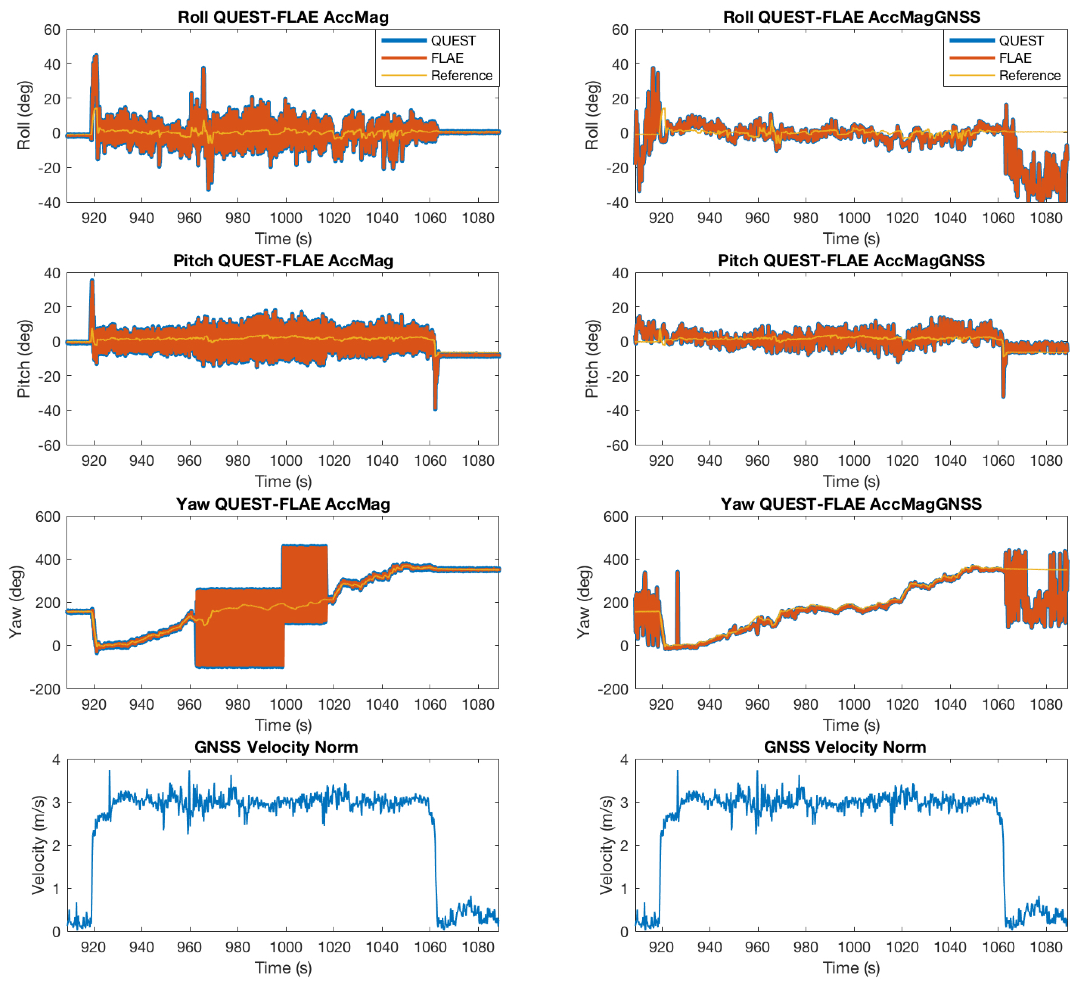
The three derived OLEQs can be used on different occasions. The OLEQ incorporates the weights so that the determination results are optimal in the sense of least-squares. With the aid of the gyroscope, the ROLEQ can achieve faster and smoother estimates. The meaning of the proposed SOLEQ is that it has a very simple linear expression that may generate short and concise analytic results for certain sensor combinations. Furthermore, when required in applications where the weights can hardly be accurately determined, e.g., vision attitude determination, the SOLEQ could be an alternative choice, as well. The attitude determination results of the three OLEQs are evaluated in the following experimental section.

5. Simulations and Experiments

5.1. Simulation: Common Cases

In this sub-section, the sensor observations are simulated with random reference vectors and true DCM in:

$${\mathbf{D}}^b={\mathbf{C}}_{true}{\mathbf{D}}^r+\epsilon$$

(86)

where $\epsilon$ is the noise item, which are not supposed to have any correlation with each other and be subject to Gaussian distribution. The reference vectors and the standard deviations of noise items are selected according to the classical test samples by Markley (see

Table 1. Test cases.

Case	Reference Vectors	Noise Standard Deviations
1	${\mathbf{D}}_1^r={[1,0,0]}^{\top },{\mathbf{D}}_2^r={[0,1,0]}^{\top },{\mathbf{D}}_3^r={[0,0,1]}^{\top }$	${\sigma }_1={10}^{-6},{\sigma }_2={10}^{-6},{\sigma }_3={10}^{-6}$
2	${\mathbf{D}}_1^r={[1,0,0]}^{\top },{\mathbf{D}}_2^r={[0,1,0]}^{\top }$	${\sigma }_1={10}^{-6},{\sigma }_2={10}^{-6}$
3	${\mathbf{D}}_1^r={[1,0,0]}^{\top },{\mathbf{D}}_2^r={[0,1,0]}^{\top },{\mathbf{D}}_3^r={[0,0,1]}^{\top }$	${\sigma }_1=0.01,{\sigma }_2=0.01,{\sigma }_3=0.01$
4	${\mathbf{D}}_1^r={[1,0,0]}^{\top },{\mathbf{D}}_2^r={[0,1,0]}^{\top }$	${\sigma }_1=0.01,{\sigma }_2=0.01$
5	${\mathbf{D}}_1^r={[0.6,0.8,0]}^{\top },{\mathbf{D}}_2^r={[0.8,-0.6,0]}^{\top }$	${\sigma }_1={10}^{-6},{\sigma }_2=0.01$
6	${\mathbf{D}}_1^r={[1,0,0]}^{\top },{\mathbf{D}}_2^r={[1,0.01,0]}^{\top },{\mathbf{D}}_3^r={[1,0,0.01]}^{\top }$	${\sigma }_1={10}^{-6},{\sigma }_2={10}^{-6},{\sigma }_3={10}^{-6}$
7	${\mathbf{D}}_1^r={[1,0,0]}^{\top },{\mathbf{D}}_2^r={[1,0.01,0]}^{\top }$	${\sigma }_1={10}^{-6},{\sigma }_2={10}^{-6}$
8	${\mathbf{D}}_1^r={[1,0,0]}^{\top },{\mathbf{D}}_2^r={[1,0.01,0]}^{\top },{\mathbf{D}}_3^r={[1,0,0.01]}^{\top }$	${\sigma }_1=0.01,{\sigma }_2=0.01,{\sigma }_3=0.01$
9	${\mathbf{D}}_1^r={[1,0,0]}^{\top },{\mathbf{D}}_2^r={[1,0.01,0]}^{\top }$	${\sigma }_1=0.01,{\sigma }_2=0.01$
10	${\mathbf{D}}_1^r={[1,0,0]}^{\top },{\mathbf{D}}_2^r={[0.96,0.28,0]}^{\top },{\mathbf{D}}_3^r={[0.96,0,0.28]}^{\top }$	${\sigma }_1={10}^{-6},{\sigma }_2=0.01,{\sigma }_3=0.01$
11	${\mathbf{D}}_1^r={[1,0,0]}^{\top },{\mathbf{D}}_2^r={[0.96,0.28,0]}^{\top }$	${\sigma }_1={10}^{-6},{\sigma }_2=0.01$
12	${\mathbf{D}}_1^r={[1,0,0]}^{\top },{\mathbf{D}}_2^r={[0.96,0.28,0]}^{\top }$	${\sigma }_1=0.01,{\sigma }_2={10}^{-6}$

), where the reference DCM ${\mathbf{C}}_{true}$ is:

$${\mathbf{C}}_{true}=\left(\begin{array}{ccc}0.352& 0.864& 0.360\\ -0.864& 0.152& 0.480\\ 0.360& -0.480& 0.800\end{array}\right)$$

(87)

Using the simulated samples, the mean attitude Root Mean Squared Errors (RMSEs) in Euler angles are evaluated with our proposed algorithms OLEQ, SOLEQ and representative algorithms including QUEST and FLAE [27], which are shown in

Table 2. Roll RMSE (deg). SOLEQ, Suboptimal Linear Estimator of Quaternion; QUEST, Shuster’s QUaternionESTimator; FLAE, Fast Linear Attitude Estimator.

Case	OLEQ	SOLEQ	QUEST	FLAE
1	$4.3516\times {10}^{-05}$	$6.1268\times {10}^{-05}$	$4.3516\times {10}^{-05}$	$4.3516\times {10}^{-05}$
2	$5.9303\times {10}^{-05}$	$6.0734\times {10}^{-05}$	$5.9303\times {10}^{-05}$	$5.9303\times {10}^{-05}$
3	$4.3482\times {10}^{-01}$	$6.0730\times {10}^{-01}$	$4.3482\times {10}^{-01}$	$4.3482\times {10}^{-01}$
4	$6.0292\times {10}^{-01}$	$6.1798\times {10}^{-01}$	$6.0292\times {10}^{-01}$	$6.0292\times {10}^{-01}$
5	$4.3313\times {10}^{-01}$	$4.3313\times {10}^{-01}$	$4.9065\times {10}^{-01}$	$2.4281\times {10}^{+01}$
6	$4.9590\times {10}^{-03}$	$3.0793\times {10}^{-01}$	$4.9590\times {10}^{-03}$	$4.9590\times {10}^{-03}$
7	$8.1132\times {10}^{-03}$	$1.3400\times {10}^{+00}$	$8.1132\times {10}^{-03}$	$8.1132\times {10}^{-03}$
8	$5.9553\times {10}^{+01}$	$6.2840\times {10}^{+01}$	$5.9553\times {10}^{+01}$	$5.9553\times {10}^{+01}$
9	$7.6662\times {10}^{+01}$	$7.6696\times {10}^{+01}$	$7.6662\times {10}^{+01}$	$7.6662\times {10}^{+01}$
10	$1.4313\times {10}^{+00}$	$1.7781\times {10}^{+00}$	$4.7663\times {10}^{+01}$	$1.5265\times {10}^{+00}$
11	$2.0254\times {10}^{+00}$	$2.0254\times {10}^{+00}$	$4.6392\times {10}^{+01}$	$2.8441\times {10}^{+00}$
12	$2.0818\times {10}^{+00}$	$2.0888\times {10}^{+00}$	$3.7218\times {10}^{+01}$	$1.7415\times {10}^{+01}$

,

Table 3. Pitch RMSE (deg).

Case	OLEQ	SOLEQ	QUEST	FLAE
1	$4.0108\times {10}^{-05}$	$5.7335\times {10}^{-05}$	$4.0108\times {10}^{-05}$	$4.0108\times {10}^{-05}$
2	$5.2860\times {10}^{-05}$	$5.6736\times {10}^{-05}$	$5.2860\times {10}^{-05}$	$5.2860\times {10}^{-05}$
3	$4.0104\times {10}^{-01}$	$5.6744\times {10}^{-01}$	$4.0104\times {10}^{-01}$	$4.0104\times {10}^{-01}$
4	$5.3887\times {10}^{-01}$	$5.7656\times {10}^{-01}$	$5.3887\times {10}^{-01}$	$5.3887\times {10}^{-01}$
5	$3.9149\times {10}^{-01}$	$3.9149\times {10}^{-01}$	$4.4335\times {10}^{-01}$	$1.2561\times {10}^{+01}$
6	$4.0121\times {10}^{-05}$	$5.7809\times {10}^{-05}$	$4.0121\times {10}^{-05}$	$4.0121\times {10}^{-05}$
7	$5.3398\times {10}^{-05}$	$5.7657\times {10}^{-05}$	$5.3398\times {10}^{-05}$	$5.3398\times {10}^{-05}$
8	$3.6755\times {10}^{-01}$	$5.7326\times {10}^{-01}$	$3.6755\times {10}^{-01}$	$3.6755\times {10}^{-01}$
9	$4.5938\times {10}^{-01}$	$5.7880\times {10}^{-01}$	$4.5938\times {10}^{-01}$	$4.5938\times {10}^{-01}$
10	$5.7186\times {10}^{-05}$	$5.7186\times {10}^{-05}$	$5.7184\times {10}^{-05}$	$5.7186\times {10}^{-05}$
11	$5.7845\times {10}^{-05}$	$5.7845\times {10}^{-05}$	$5.7846\times {10}^{-05}$	$5.7844\times {10}^{-05}$
12	$4.9161\times {10}^{-01}$	$5.7554\times {10}^{-01}$	$7.9376\times {10}^{+00}$	$3.9359\times {10}^{+00}$

and

Table 4. Yaw RMSE (deg).

Case	OLEQ	SOLEQ	QUEST	FLAE
1	$4.3587\times {10}^{-05}$	$6.1084\times {10}^{-05}$	$4.3587\times {10}^{-05}$	$4.3587\times {10}^{-05}$
2	$4.8694\times {10}^{-05}$	$6.1015\times {10}^{-05}$	$4.8694\times {10}^{-05}$	$4.8694\times {10}^{-05}$
3	$4.4127\times {10}^{-01}$	$6.0868\times {10}^{-01}$	$4.4127\times {10}^{-01}$	$4.4127\times {10}^{-01}$
4	$4.8593\times {10}^{-01}$	$6.1289\times {10}^{-01}$	$4.8593\times {10}^{-01}$	$4.8593\times {10}^{-01}$
5	$2.5186\times {10}^{-01}$	$2.5186\times {10}^{-01}$	$2.8536\times {10}^{-01}$	$1.7459\times {10}^{+01}$
6	$3.6421\times {10}^{-05}$	$6.1651\times {10}^{-05}$	$3.6421\times {10}^{-05}$	$3.6421\times {10}^{-05}$
7	$4.8748\times {10}^{-05}$	$6.0826\times {10}^{-05}$	$4.8748\times {10}^{-05}$	$4.8748\times {10}^{-05}$
8	$3.9812\times {10}^{-01}$	$6.1557\times {10}^{-01}$	$3.9812\times {10}^{-01}$	$3.9812\times {10}^{-01}$
9	$4.9366\times {10}^{-01}$	$6.1163\times {10}^{-01}$	$4.9366\times {10}^{-01}$	$4.9366\times {10}^{-01}$
10	$6.1834\times {10}^{-05}$	$6.1834\times {10}^{-05}$	$6.1836\times {10}^{-05}$	$6.1844\times {10}^{-05}$
11	$6.2069\times {10}^{-05}$	$6.2069\times {10}^{-05}$	$6.2069\times {10}^{-05}$	$6.2077\times {10}^{-05}$
12	$3.1726\times {10}^{-01}$	$6.1275\times {10}^{-01}$	$5.1968\times {10}^{+00}$	$2.8814\times {10}^{+00}$

.

Table 5. Loss function values.

Case	OLEQ	SOLEQ	QUEST	FLAE
1	$5.0651\times {10}^{-13}$	$1.0130\times {10}^{-12}$	$5.0651\times {10}^{-13}$	$5.0651\times {10}^{-13}$
2	$2.4901\times {10}^{-13}$	$4.9802\times {10}^{-13}$	$2.4901\times {10}^{-13}$	$2.4901\times {10}^{-13}$
3	$4.9338\times {10}^{-05}$	$9.8666\times {10}^{-05}$	$4.9338\times {10}^{-05}$	$4.9338\times {10}^{-05}$
4	$2.5369\times {10}^{-05}$	$5.0736\times {10}^{-05}$	$2.5369\times {10}^{-05}$	$2.5369\times {10}^{-05}$
5	$5.0582\times {10}^{-13}$	$5.0582\times {10}^{-13}$	$6.5095\times {10}^{-13}$	$8.5878\times {10}^{-10}$
6	$5.0422\times {10}^{-13}$	$9.4333\times {10}^{-10}$	$5.0422\times {10}^{-13}$	$5.0422\times {10}^{-13}$
7	$2.4728\times {10}^{-13}$	$8.8239\times {10}^{-09}$	$2.4728\times {10}^{-13}$	$2.4728\times {10}^{-13}$
8	$4.8216\times {10}^{-05}$	$1.1593\times {10}^{-04}$	$4.8216\times {10}^{-05}$	$4.8216\times {10}^{-05}$
9	$2.5327\times {10}^{-05}$	$5.0651\times {10}^{-05}$	$2.5327\times {10}^{-05}$	$2.5327\times {10}^{-05}$
10	$1.4827\times {10}^{-12}$	$1.7575\times {10}^{-12}$	$4.8431\times {10}^{-10}$	$1.7195\times {10}^{-12}$
11	$4.8573\times {10}^{-13}$	$4.8573\times {10}^{-13}$	$2.4106\times {10}^{-10}$	$9.2333\times {10}^{-13}$
12	$5.0105\times {10}^{-13}$	$5.0105\times {10}^{-05}$	$1.3143\times {10}^{-10}$	$3.4336\times {10}^{-11}$

contains the computed average Wahba’s loss function values for different cases and algorithms. These algorithms are executed with MATLAB r2016 software (r2016, MathWorks, Natick, USA) on a PC 10,000 times with each data sample.

We first observe the attitude RMSEs. From the results of OLEQ, QUEST and FLAE, it is noticeable that they have a similar attitude determination accuracy. Combining the same statistics in Table 5, the proposed OLEQ is well verified for its optimality. From the presented results, we see that SOLEQ has larger attitude errors and loss function values compared to the other optimal methods. The proposed SOLEQ is sub-optimal as it actually approximates the attitude estimator where the weights are ignored. Therefore, this simulation scenario has validated the correctness and optimality of the proposed OLEQ and SOLEQ.

5.2. Simulation: Extreme Cases

$$\begin{array}{c}{\mathbf{D}}_1^r=\left(\begin{array}{c}1\\ 0\\ 0\end{array}\right),{\mathbf{D}}_2^r=\left(\begin{array}{c}-0.99712\\ 0.07584\\ 0\end{array}\right),{\mathbf{D}}_3^r=\left(\begin{array}{c}-0.99712\\ -0.07584\\ 0\end{array}\right)\hfill \\ {\sigma }_1=1arcsec,{\sigma }_2={\sigma }_3=1deg\hfill \end{array}$$

(88)

Conventional Wahba’s solutions face a dilemma when exposed to some critical pairs of vector observations. For instance, Markley and Mortari give an example where the sensors are configured by Equation (88) [37]. In such a scenario, the root of the characteristic polynomial of the Davenport matrix cannot be easily obtained by Newton iterations. The internal reason is given by Cheng [44] showing that it results in numerical loss according to the specific CPU word storage length. A flexible transformation of the characteristic polynomial is proposed then to significantly boost the convergence. As such configurations indeed happen in engineering practice, there is a necessity to evaluate the proposed schemes by comparisons with representative solvers. With similar simulation techniques as previously mentioned, the vectors are simulated with given reference vectors and standard deviations by rotation of ${\mathbf{C}}_{true}$. Here, the QUEST algorithm is revised to Cheng’s form. First, we mainly compare the two iterative methods QUEST and OLEQ because in our existing paper [27], QUEST and FLAE have been proven to have a very similar behaviour when faced with this extreme case. Here, the iteration stops when the Euclidean norm of the neighbouring attitude quaternion difference is less than $1\times {10}^{-8}$. For QUEST, the maximum iteration number is set to 50. The obtained results are depicted in Figure 1. We can see that the supervised QUEST can obtain accurate quaternion solutions within several iterations. Actually, before Cheng’s improvement, QUEST may exceed the maximum iteration number from time to time. The proposed OLEQ, however, shows better performance dealing with this extreme case. Furthermore, the final mean loss function values of the two algorithms are computed as $4.9890\times {10}^{-11}$ and $2.8391\times {10}^{-10}$, which reveals that the proposed OLEQ can not only obtain faster solutions, but leads to smaller loss function values, compared with supervised QUEST. As is known to everyone, QUEST is the most representative Wahba’s solution using Davenport’s q-method. Many other algorithms like ESOQand FOAMactually have the same performance as QUEST. Therefore, in this way, OLEQ is proven to be faster and much more robust than the whole class of algorithms based on Davenport’s q-method. This also shows that the presented novel attitude evolution method owns brand new abilities.

5.3. Experiment: Accelerometer-Magnetometer Case

In this sub-section, we conduct an experiment where the accelerometer-magnetometer combination is adopted. Such a sensor combination is extensively applied nowadays in low-cost attitude estimation schemes. The accelerometer is pre-calibrated using six-direction bias cancelling, while the magnetometer is calibrated using the method proposed by Y . Wu et al. [45].

The hardware is constituted by a battery, a high-end Attitude and Heading Reference System (AHRS) with a high precision internal accelerometer, magnetometer and gyroscope, a transmitter for remote data transmission and a micro-controller for the implementation of the algorithm using the C++ language on the FreeRTOS. With the designed hardware platform shown in Figure 2, we collect a dataset with 10,000 samples.

The main purpose of this sub-section is to validate the performances of the proposed OLEQ, SOLEQ and ROLEQ since the AHRS has angular rate readouts. The compared results with the reference angles from representative methods are obtained (see Figure 3, Figure 4 and Figure 5). Note that here, the weights between the accelerometer and magnetometer for Wahba’s solution are chosen as 0.63 and 0.37 according to their respective noise characteristics. Yet, the local magnetometer’s reference vector is calculated as ${\mathbf{M}}^r={\left(0.60311,0,-0.79766\right)}^{\top }$ in Wuxi, Jiangsu Province, China.

In Figure 3, the reference angles, QUEST solutions and SOLEQ solutions have been presented. The results indicate that the proposed sub-optimal estimator can estimate the attitude angles with similar macroscopic accuracy. Detailed attitude errors are plotted in Figure 4 and Figure 5. It is noticed that in general, these algorithms have the same errors with respect to the reference. Figure 5 shows that the overall attitude accuracy of ROLEQ is slightly smaller than the others. This is because it is first processed using the angular rate data, which essentially plays the role of a smoothing procedure.

5.4. Experiment: GNSS-Aided Attitude Determination for Land Vehicles

The GNSS receiver is widely employed in the attitude determination tasks for land and unmanned aerial vehicles. In this experiment, we use a designed rover (see Figure 6) to validate the feasibility of the proposed algorithm for GNSS attitude determination.

The rover is equipped with the aforementioned navigation computer and employs an external ublox M8N GNSS module with a serial-com connection to the board at the sampling frequency of 5 Hz. This rover is controlled by a handheld 2.4-GHz transmitter, and the onboard Pixhawk autopilot generates PID controlling commands to the servos and motors according to internal measurements. In this experiment, the rover is ran on a playground of UESTC, and we pick up one period of data in which the GNSS velocity is valid. In the data history, the magnetometer was distorted by outer unknown electromagnetic and ferromagnetic fields. Furthermore, during the execution process, raw measurements from the gyroscope and accelerometer are also logged with a speed of 250 Hz. The raw data are shown in Figure 7.

According to the sensor noise characteristics, the weights of the accelerometer-magnetometer combination are 0.9 and 0.1, respectively; while for the accelerometer-magnetometer-GNSS combination, the weights are chosen as 0.474, 0.05 and 0.474, respectively. The reference vector of the magnetometer is determined by the initial GNSS positioning results with the IGRF model [35]. By making use of algorithms including QUEST, FLAE, OLEQ and SOLEQ, the computation results are summarized in Figure 8 and Figure 9.

We specifically add the GNSS velocity norm under the Euler angle results to illustrate the influence of the velocity scalar on the attitude determination results. In principle, when the vehicle is not moving with relative discriminative velocities, the GNSS receiver cannot give accurate speed estimates. Therefore, it is shown in the initial stage of the attitude determination results where the GNSS takes part, in that the determination accuracy of the yaw angle is seemingly very poor. As the velocity increases, the accuracy is improved very quickly accordingly. The accelerometer-magnetometer combination is largely distorted by magnetic disturbances. The integrated results of roll, pitch and, moreover, the yaw angles are influenced, generating very obvious differences with reference angles. With the aid of GNSS velocity, the corresponding attitude determination accuracy is not damaged because Wahba’s solution balances the sensor inputs by the weights. It is observed that the OLEQ is validated to have almost the same accuracy for normal sensors in the aforementioned section, and in this section, such behaviour holds, as well. The SOLEQ, however, does not employ the weights and therefore produces relatively worse estimates, but for GNSS case, it is still better than the accelerometer-magnetometer estimates. The RMSEs of these scenarios are shown in

Table 6. RMSEs of the experiment (in deg).

Roll Case	OLEQ	SOLEQ	QUEST	FLAE
Acc-MagExperiment	$17.2$	$16.8$	$17.2$	$17.2$
Acc-Mag-GNSS Experiment	$10.1$	$9.7$	$10.2$	$10.2$
Pitch Case	OLEQ	SOLEQ	QUEST	FLAE
Acc-Mag Experiment	$15.9$	$14.6$	$15.9$	$15.9$
Acc-Mag-GNSS Experiment	$14.4$	$13.2$	$14.4$	$14.4$
Yaw Case	OLEQ	SOLEQ	QUEST	FLAE
Acc-Mag Experiment	$154.3$	$155.9$	$154.3$	$154.3$
Acc-Mag-GNSS Experiment	$16.7$	$44.8$	$16.7$	$16.7$

. The results demonstrate to us the validity of the proposed algorithms, especially OLEQ.

5.5. Computation Time

From another point of view, the time consumption of various algorithms needs to be investigated. The time consumption is assessed on the embedded platform with the C++ programming language to ensure fairness. A rough evaluation is done with two pairs of vector observations in a few samples, which shows direct time consumption results (see Figure 10). As shown in the figure, for two pairs of vector observations, the three proposed algorithms’ computation times are between QUEST and FLAE. However, from the expressions of the algorithms presented before, the number of vector observations is influential with respect to the final time consumption. Hence, with the simulation samples, each algorithm is again tested 20,000-times with different vector observation numbers. The time consumption is averaged and plotted in Figure 11. The results indicate that the algorithms are all linear, owning time complexities of $O\left(n\right)$. QUEST, OLEQ and ROLEQ join at the vector observation number of 20. For common tasks, such a number covers most amounts of sensors. Although FLAE has the least time consumption, it can not overcome the drawbacks of extreme cases as well as OLEQ. That is to say, the proposed algorithms can replace the original algorithms for faster and more robust attitude determination.

6. Conclusions

This paper revisits the attitude determination from vector observations for a GNSS/AM case study. Novel linear algorithms are designed to obtain accurate attitude estimates in the sense of least-squares. Handling it in this manner, the computed quaternion is identical or suboptimal with respect to the conventional Wahba’s solutions including QUEST and FLAE. We have found out that:

• Numerical simulations exhibit that the proposed OLEQs have a similar accuracy with representative solvers.
• It is also demonstrated that faced with extreme cases, OLEQs show much more robustness with less computation iterations.
• The computation speeds of OLEQs are tested, revealing that they belong to computationally-efficient algorithms.
• Moreover, a real vehicular experiment of a GNSS/AM system is designed and conducted showing the effectiveness of the proposed OLEQs in real-world embedded applications.

The MATLAB source codes of the proposed algorithms are uploaded as open-source files at https://github.com/zarathustr/OLEQs. The presented approach provides the reader with a brand new viewpoint of attitude evolution and hopefully will benefit related multi-sensor attitude determination applications.

References

1. Zhou, Z.; Li, Y.; Liu, J.; Li, G. Equality constrained robust measurement fusion for adaptive kalman-filter-based heterogeneous multi-sensor navigation. IEEE Trans. Aerosp. Electron. Syst. 2013, 49, 2146–2157. [Google Scholar]
2. Zhou, Z.; Li, Y.; Zhang, J.; Rizos, C. Integrated Navigation System for a Low-Cost Quadrotor Aerial Vehicle in the Presence of Rotor Influences. J. Surv. Eng. 2017, 143, 05016006. [Google Scholar] [CrossRef]
3. Chang, G.; Xu, T.; Wang, Q. M-estimator for the 3D symmetric Helmert coordinate transformation. J. Geod. 2017, 92, 47–58. [Google Scholar] [CrossRef]
4. Wu, Y.; Wang, J.; Hu, D. A New Technique for INS/GNSS Attitude and Parameter Estimation Using Online Optimization. IEEE Trans. Signal Process. 2014, 62, 2642–2655. [Google Scholar] [CrossRef]
5. Chang, L.; Qin, F.; Zha, F. Pseudo Open-Loop Unscented Quaternion Estimator for Attitude Estimation. IEEE Sens. J. 2016, 16, 4460–4469. [Google Scholar] [CrossRef]
6. Han, S.; Wang, J. Quantization and colored noises error modeling for inertial sensors for GPS/INS integration. IEEE Sens. J. 2011, 11, 1493–1503. [Google Scholar] [CrossRef]
7. Chang, L.; Li, J.; Chen, S. Initial Alignment by Attitude Estimation for Strapdown Inertial Navigation Systems. IEEE Trans. Instrum. Meas. 2015, 64, 784–794. [Google Scholar] [CrossRef]
8. Marins, J.; Yun, X.; Bachmann, E.; McGhee, R.; Zyda, M. An extended Kalman filter for quaternion-based orientation estimation using MARG sensors. In Proceedings of the 2001 IEEE/RSJ International Conference on Intelligent Robots and Systems. Expanding the Societal Role of Robotics in the the Next Millennium (Cat. No.01CH37180), Maui, HI, USA, 29 October–3 November 2001; Volume 4. [Google Scholar]
9. Tian, Y.; Wei, H.; Tan, J. An adaptive-gain complementary filter for real-time human motion tracking with MARG sensors in free-living environments. IEEE Trans. Neural Syst. Rehabil. Eng. 2013, 21, 254–264. [Google Scholar] [CrossRef] [PubMed]
10. Wu, J.; Zhou, Z.; Li, R.; Yang, L.; Fourati, H. Attitude Determination Using a Single Sensor Observation : Analytic Quaternion Solutions and Property Discussion. IET Sci. Meas. Technol. 2017, 11, 731–739. [Google Scholar] [CrossRef]
11. Du, S.; Gao, Y. Inertial aided cycle slip detection and identification for integrated PPP GPS and INS. Sensors 2012, 12, 14344–14362. [Google Scholar] [CrossRef] [PubMed]
12. Aleshechkin, A. Algorithm of GNSS-based attitude determination. Gyroscopy Navig. 2011, 2, 269. [Google Scholar] [CrossRef]
13. Grewal, M.; Andrews, A. Kalman Filtering: Theory and Practice Using MATLAB; John Wiley & Sons: Hoboken, NJ, USA, 2001. [Google Scholar]
14. Niu, X.; Nassar, S.; El-Sheimy, N. An Accurate Land-Vehicle MEMS IMU/GPS Navigation System Using 3D Auxiliary Velocity Updates. Navigation 2007, 54, 177–188. [Google Scholar] [CrossRef]
15. Niu, X.; Nasser, S.; Goodall, C.; El-Sheimy, N. A universal approach for processing any MEMS inertial sensor configuration for land-vehicle navigation. J. Navig. 2007, 60, 233–245. [Google Scholar] [CrossRef]
16. Gebre-Egziabher, D.; Elkaim, G.H. MAV attitude determination by vector matching. IEEE Trans. Aerosp. Electron. Syst. 2008, 44. [Google Scholar] [CrossRef]
17. Zhang, J.; Zhang, K.; Grenfell, R.; Deakin, R. Short note: On the relativistic Doppler effect for precise velocity determination using GPS. J. Geod. 2006, 80, 104–110. [Google Scholar] [CrossRef]
18. Zhou, Z.; Li, B. Optimal Doppler-aided smoothing strategy for GNSS navigation. GPS Solut. 2017, 21, 197–210. [Google Scholar]
19. Geng, J.; Bock, Y.; Melgar, D.; Crowell, B.W.; Haase, J.S. A new seismogeodetic approach applied to GPS and accelerometer observations of the 2012 Brawley seismic swarm: Implications for earthquake early warning. Geochem. Geophys. Geosyst. 2013, 14, 2124–2142. [Google Scholar] [CrossRef]
20. Geng, J.; Melgar, D.; Bock, Y.; Pantoli, E.; Restrepo, J. Recovering coseismic point ground tilts from collocated high-rate GPS and accelerometers. Geophys. Res. Lett. 2013, 40, 5095–5100. [Google Scholar] [CrossRef]
21. Wahba, G. A Least Squares Estimate of Satellite Attitude. SIAM Rev. 1965, 7, 409. [Google Scholar] [CrossRef]
22. Shuster, M.D.; Oh, S.D. Three-axis attitude determination from vector observations. J. Guid. Control Dyn. 1981, 4, 70–77. [Google Scholar] [CrossRef]
23. Markley, F.L. Attitude Determination using Vector Observations and the Singular Value Decomposition. J. Astronaut. Sci. 1988, 36, 245–258. [Google Scholar]
24. Mortari, D. ESOQ: A Closed-Form Solution to the Wahba Problem. J. Astronaut. Sci. 1997, 45, 195–204. [Google Scholar]
25. Davenport, P.B. A Vector Approach to the Algebra of Rotations with Applications; Technical Report August; National Aeronautics and Space Administration: Washington, DC, USA, 1968.
26. Chang, G.; Xu, T.; Wang, Q. Error analysis of Davenport’s q method. Automatica 2017, 75, 217–220. [Google Scholar] [CrossRef]
27. Wu, J.; Zhou, Z.; Gao, B.; Li, R.; Cheng, Y.; Fourati, H. Fast Linear Quaternion Attitude Estimator Using Vector Observations. IEEE Trans. Autom. Sci. Eng. 2018, 15, 307–319. [Google Scholar] [CrossRef]
28. Yang, Y.; Zhou, Z. An analytic solution to Wahbas problem. Aerosp. Sci. Technol. 2013, 30, 46–49. Available online: http://xxx.lanl.gov/abs/1309.5679 (accessed on 24 February 2018). [CrossRef]
29. Yang, Y. Attitude determination using Newton’s method on Riemannian manifold. Proc. Inst. Mech. Eng. Part G J. Aerosp. Eng. 2015, 229, 2737–2742. [Google Scholar] [CrossRef]
30. Forbes, J.R.; de Ruiter, A.H.J. Linear-Matrix-Inequality-Based Solution to Wahba’s Problem. J. Guid. Control Dyn. 2015, 38, 147–151. [Google Scholar]
31. Mahony, R.; Hamel, T.; Pflimlin, J.M. Nonlinear complementary filters on the special orthogonal group. IEEE Trans. Autom. Control 2008, 53, 1203–1218. [Google Scholar] [CrossRef] [Green Version]
32. Madgwick, S.O.H.; Harrison, A.J.L.; Vaidyanathan, R. Estimation of IMU and MARG orientation using a gradient descent algorithm. In Proceedings of the IEEE International Conference on Rehabilitation Robotics, Zurich, Switzerland, 29 June–1 July 2011. [Google Scholar]
33. Arun, K.S.; Huang, T.S.; Blostein, S.D. Least-Squares Fitting of Two 3-D Point Sets. IEEE Trans. Pattern Anal. Mach. Intell. 1987, PAMI-9, 698–700. [Google Scholar] [CrossRef]
34. Ye, C.; Hong, S.; Tamjidi, A. 6-DOF Pose Estimation of a Robotic Navigation Aid by Tracking Visual and Geometric Features. IEEE Trans. Autom. Sci. Eng. 2015, 12, 1169–1180. [Google Scholar] [CrossRef] [PubMed]
35. Abdelrahman, M.; Park, S.Y. Simultaneous spacecraft attitude and orbit estimation using magnetic field vector measurements. Aerosp. Sci. Technol. 2011, 15, 653–669. [Google Scholar] [CrossRef]
36. Markley, F.L.; Mortari, D. Quaternion attitude estimation using vector observations. J. Astronaut. Sci. 2000, 48, 359–380. [Google Scholar]
37. Markley, F.L.; Mortari, D. How to estimate attitude from vector observations. Adv. Astronaut. Sci. 2000, 103, 1979–1996. [Google Scholar]
38. Markley, F.L. Humble problems. Adv. Astronaut. Sci. 2006, 124 II, 2205–2222. [Google Scholar]
39. Wu, J.; Zhou, Z.; Chen, J.; Fourati, H.; Li, R. Fast Complementary Filter for Attitude Estimation Using Low-Cost MARG Sensors. IEEE Sens. J. 2016, 16, 6997–7007. [Google Scholar] [CrossRef]
40. Shuster, M.D. Filter QUEST or REQUEST. J. Guid. Control Dyn. 2009, 32, 643–645. [Google Scholar] [CrossRef]
41. Valenti, R.G.; Dryanovski, I.; Xiao, J. A Linear Kalman Filter for MARG Orientation Estimation Using the Algebraic Quaternion Algorithm. IEEE Trans. Instrum. Meas. 2016, 65, 467–481. [Google Scholar] [CrossRef]
42. Horn, R.A.; Johnson, C.R. Matrix Analysis; Cambridge University Press: Cambridge, UK, 2012. [Google Scholar]
43. Yang, Y. Spacecraft attitude determination and control: Quaternion based method. Annu. Rev. Control 2012, 36, 198–219. [Google Scholar] [CrossRef]
44. Cheng, Y.; Shuster, M.D. Improvement to the Implementation of the QUEST Algorithm. J. Guid. Control Dyn. 2014, 37, 301–305. [Google Scholar] [CrossRef]
45. Wu, Y.; Shi, W. On Calibration of Three-Axis Magnetometer. IEEE Sens. J. 2015, 15, 6424–6431. [Google Scholar] [CrossRef]
Figure 1. Iteration numbers of QUEST and OLEQ when faced with an extreme case.
Remotesensing 10 00377 g001
Figure 2. Designed hardware for the implementation of the algorithm.
Remotesensing 10 00377 g002
Figure 3. Experiment
Remotesensing 10 00377 g003
Figure 4. Experiment results of OLEQ, SOLEQ and representative algorithms using sampled data and different algorithms.
Remotesensing 10 00377 g004
Figure 5. Experiment results of Recursive OLEQ (ROLEQ) and representative algorithms using sampled data and different algorithms.
Remotesensing 10 00377 g005
Figure 6. The designed multi-functional rover for the validation of the proposed algorithms.
Remotesensing 10 00377 g006
Figure 7. Raw sensor measurements from the memory logging.
Remotesensing 10 00377 g007
Figure 8. Attitude determination from the accelerometer, magnetometer and velocity output of the GNSS receiver, by means of QUEST and FLAE.
Remotesensing 10 00377 g008
Figure 9. Attitude determination from the accelerometer, magnetometer and velocity output of the GNSS receiver, by means of OLEQ and SOLEQ.
Remotesensing 10 00377 g009
Figure 10. Time consumption of various algorithms.
Remotesensing 10 00377 g010
Figure 11. Time consumption of algorithms with respect to the number of vector observations.
Remotesensing 10 00377 g011