A Relative Radiometric Calibration Method Based on the Histogram of Side-Slither Data for High-Resolution Optical Satellite Imagery


Abstract
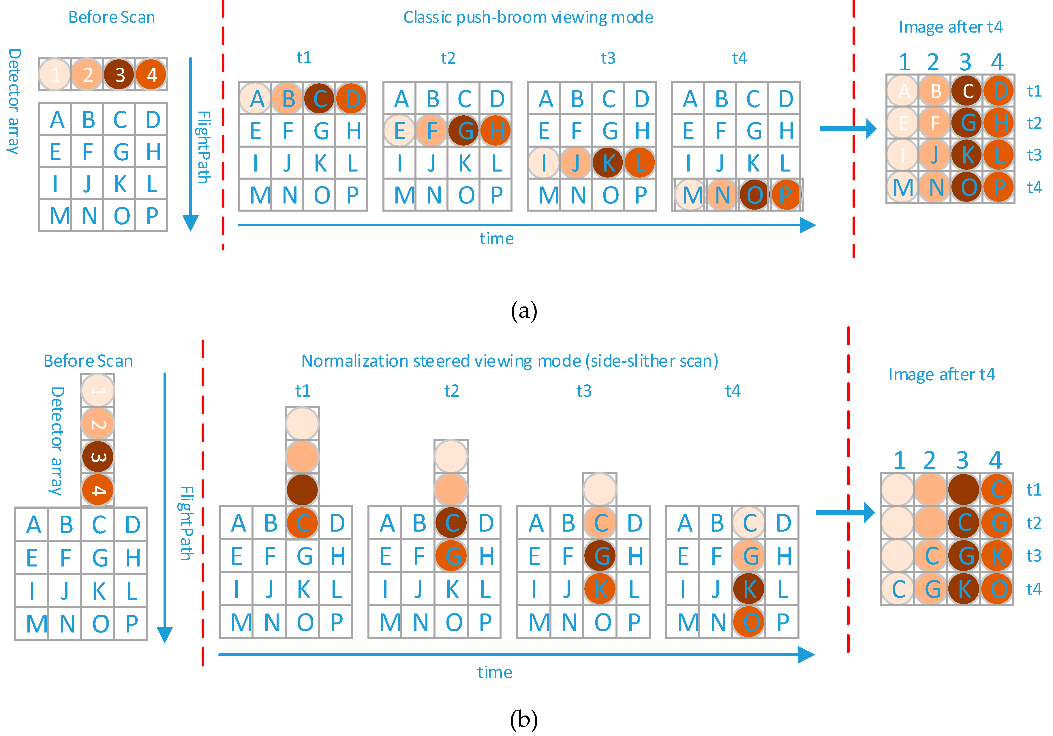
:1. Introduction
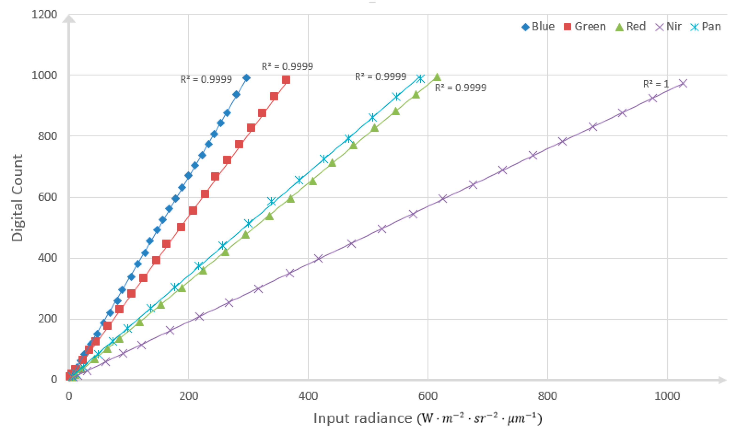
2. The Model of Relative Radiometric Correction
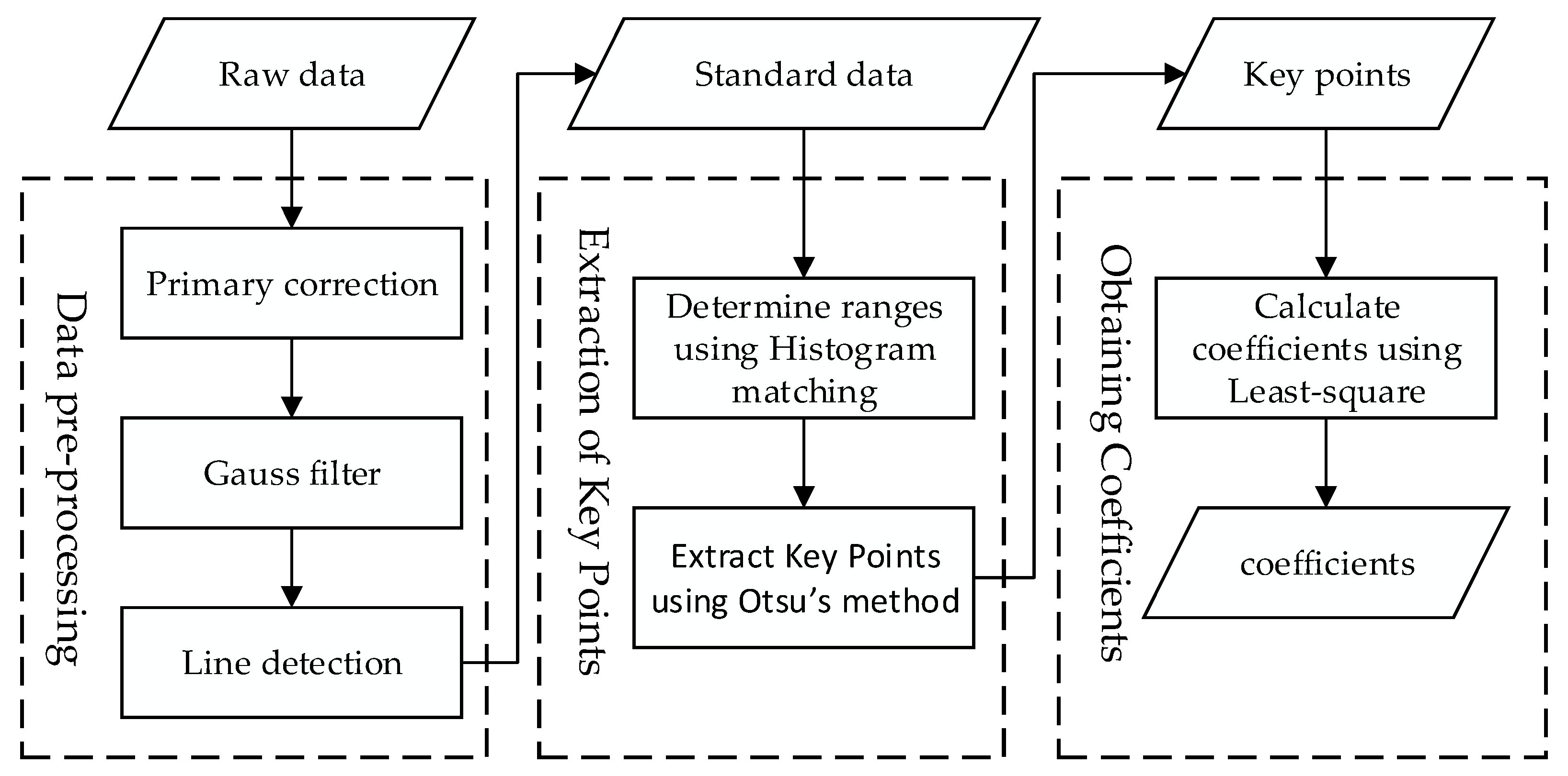
3. Methods
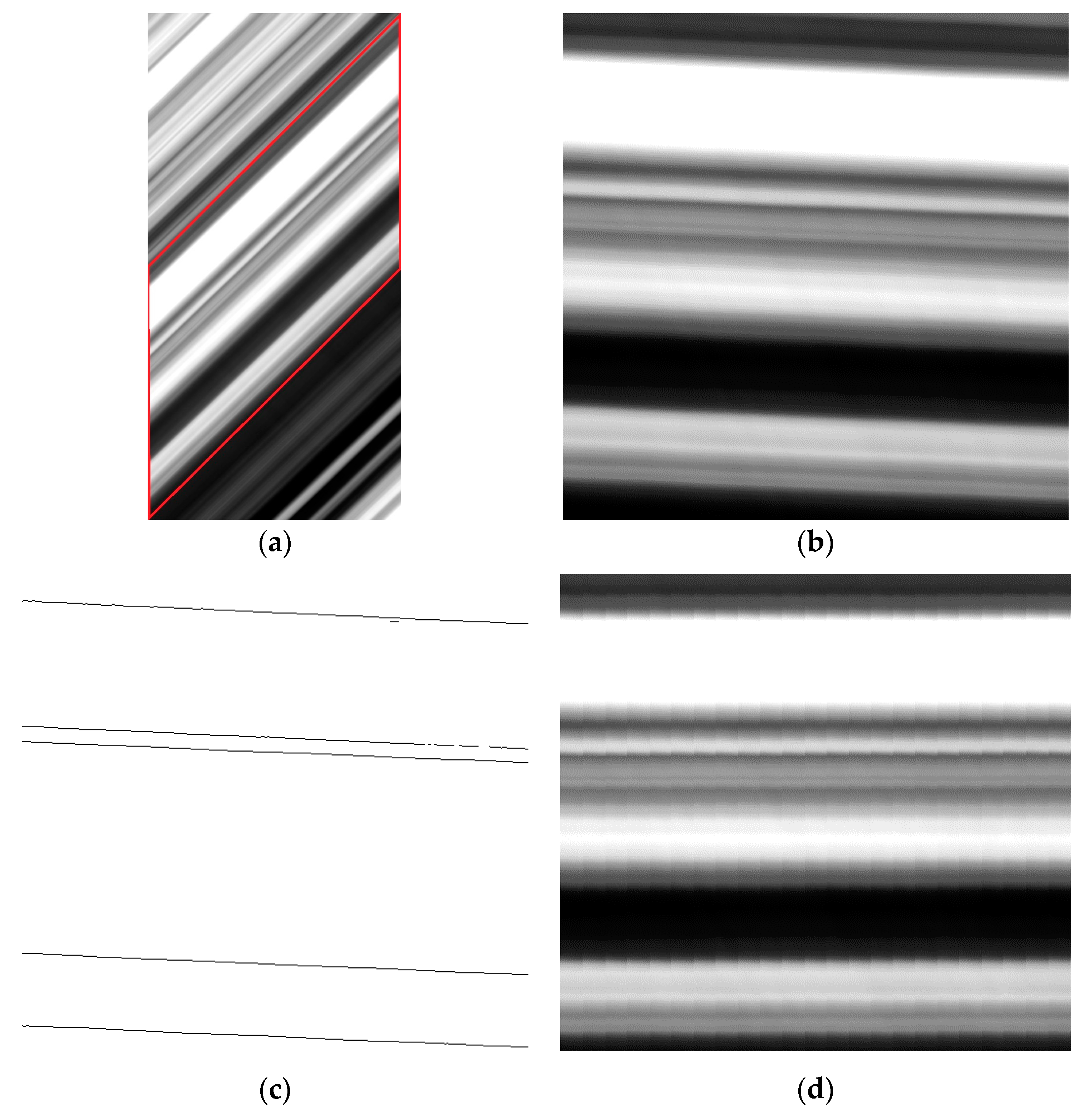
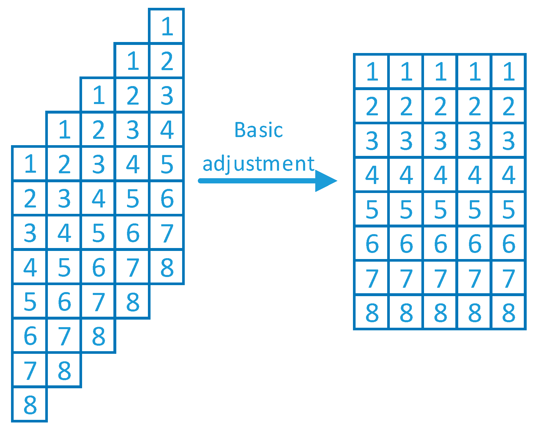
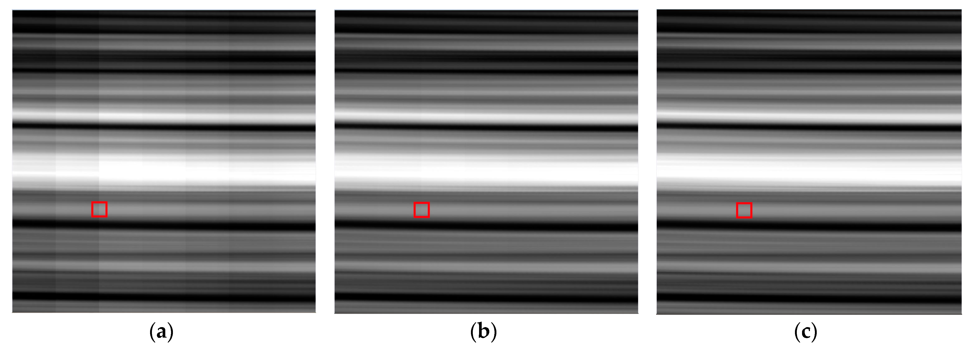
3.1. Pre-Processing
3.2. Extraction of Key Points
3.2.1. Histogram Matching
3.2.2. Otsu’s Method
3.3. Obtaining Coefficients
3.4. Processing of the Proposed Method
- Definition of n different DN values in the range in the whole image.
- For the -th detector:
- A normalization look-up table was created to map every DN to a referenced DN through histogram matching.
- Obtain n different DN values , locating the corresponding value of in the look-up table.
- Based on the n different DN values , construct ranges .
- For each range , obtain the maximum between-class variance point using Otsu’s method.
- In step 2, m points were obtained for the -th detector. Suppose the number of detectors is N, then for index k, the average response is .
- For the -th detector, the relative radiometric coefficients were obtained by minimizing ;
4. Results
4.1. Experimental Data
4.2. Accuracy Assessment
4.2.1. Relative Radiometric Accuracy Indices
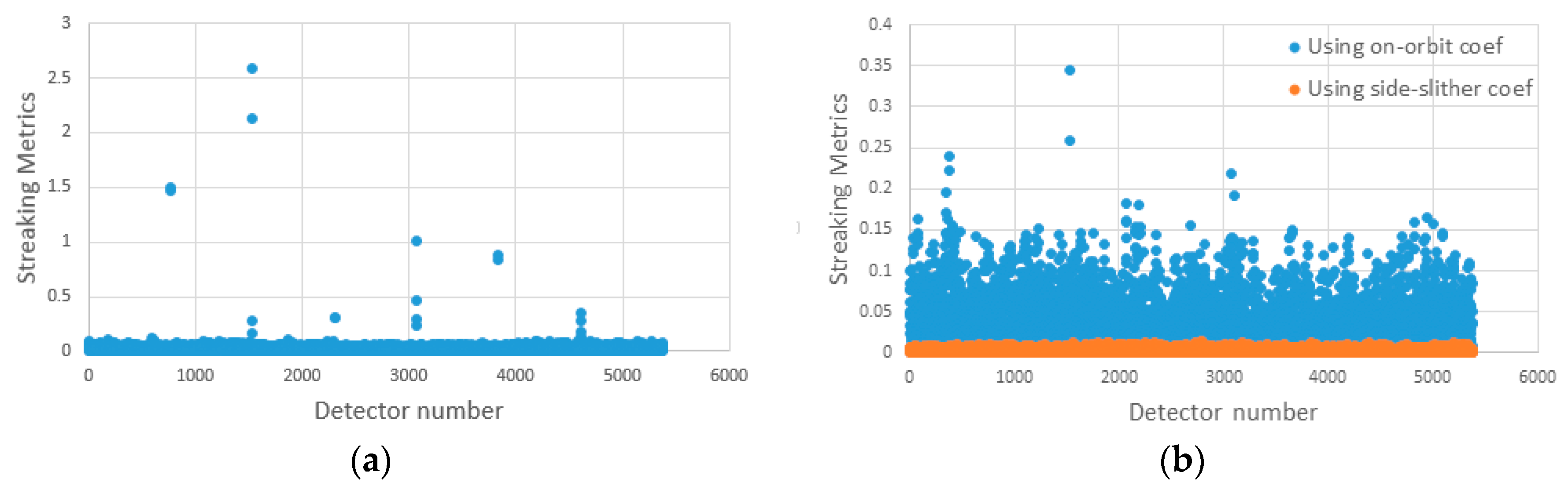
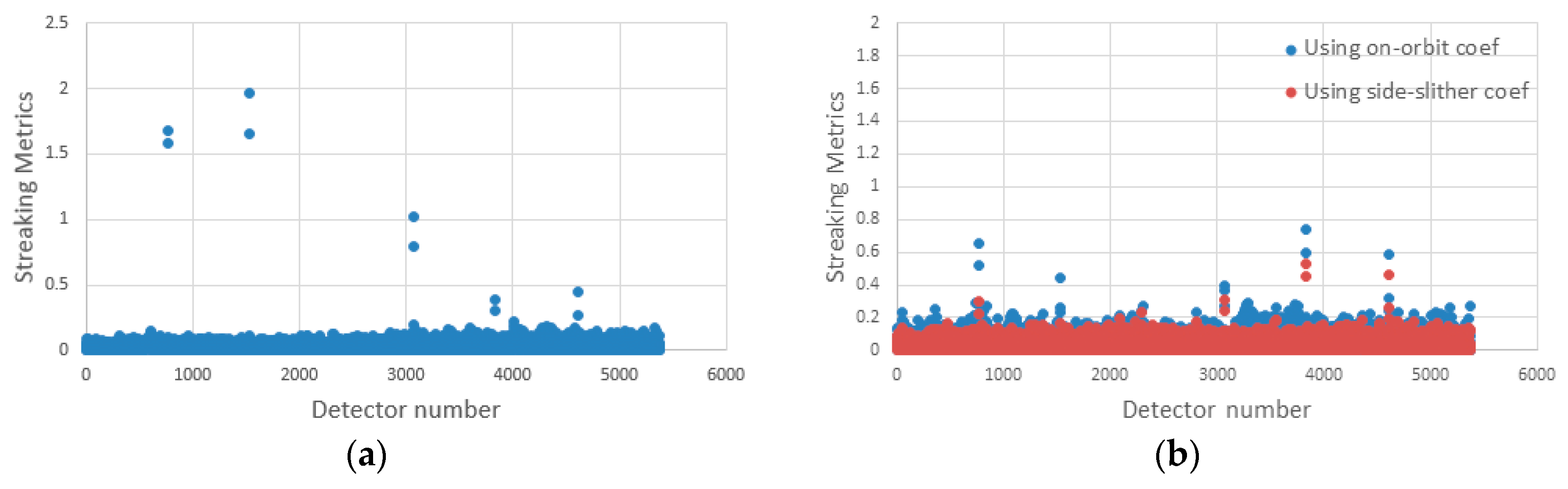
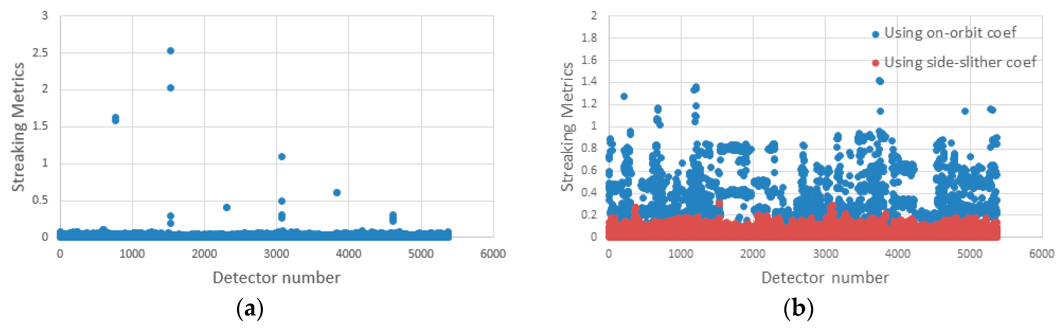
4.2.2. Streaking Metrics
4.2.3. Improvement Factor (IF)
4.2.4. Structural Similarity Index (SSIM)
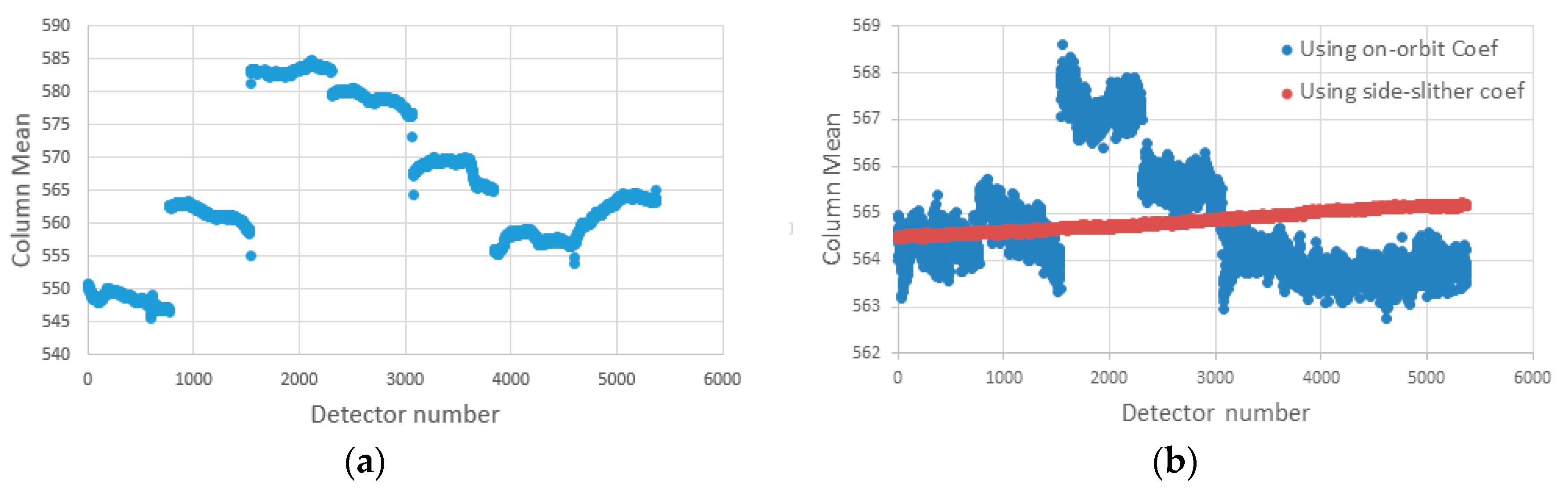
4.3. Verification Results for Raw Image in Group B
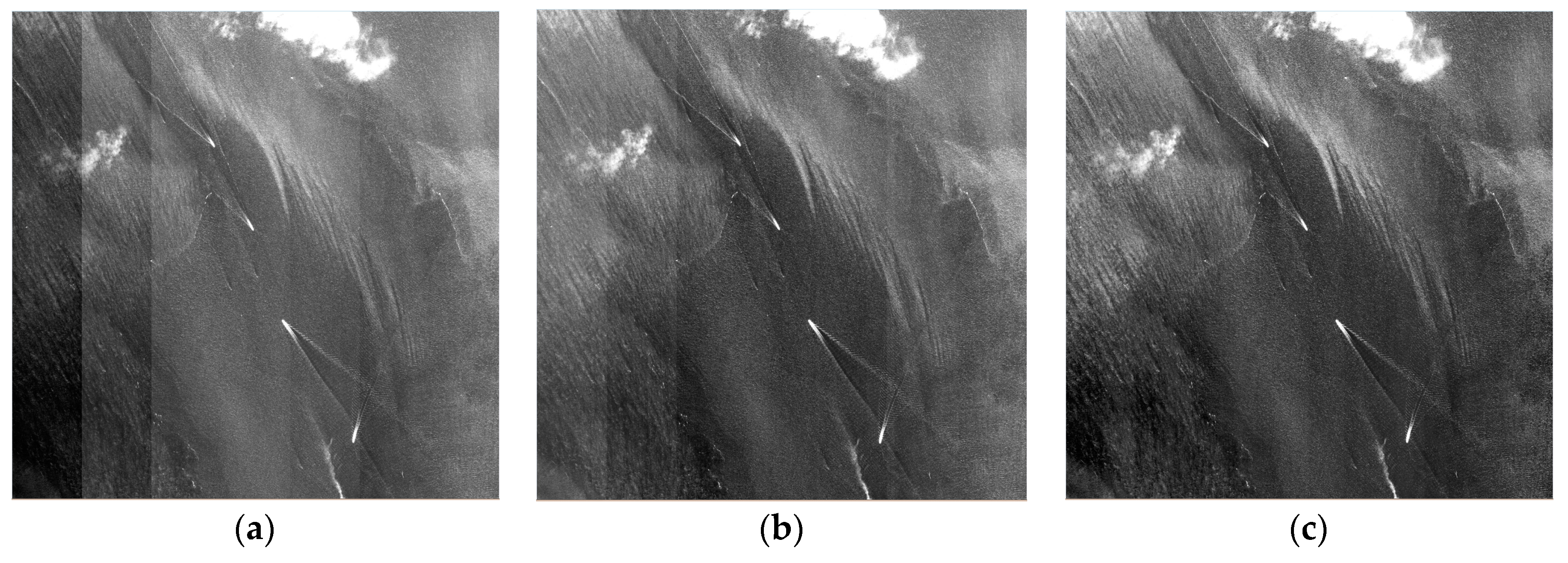
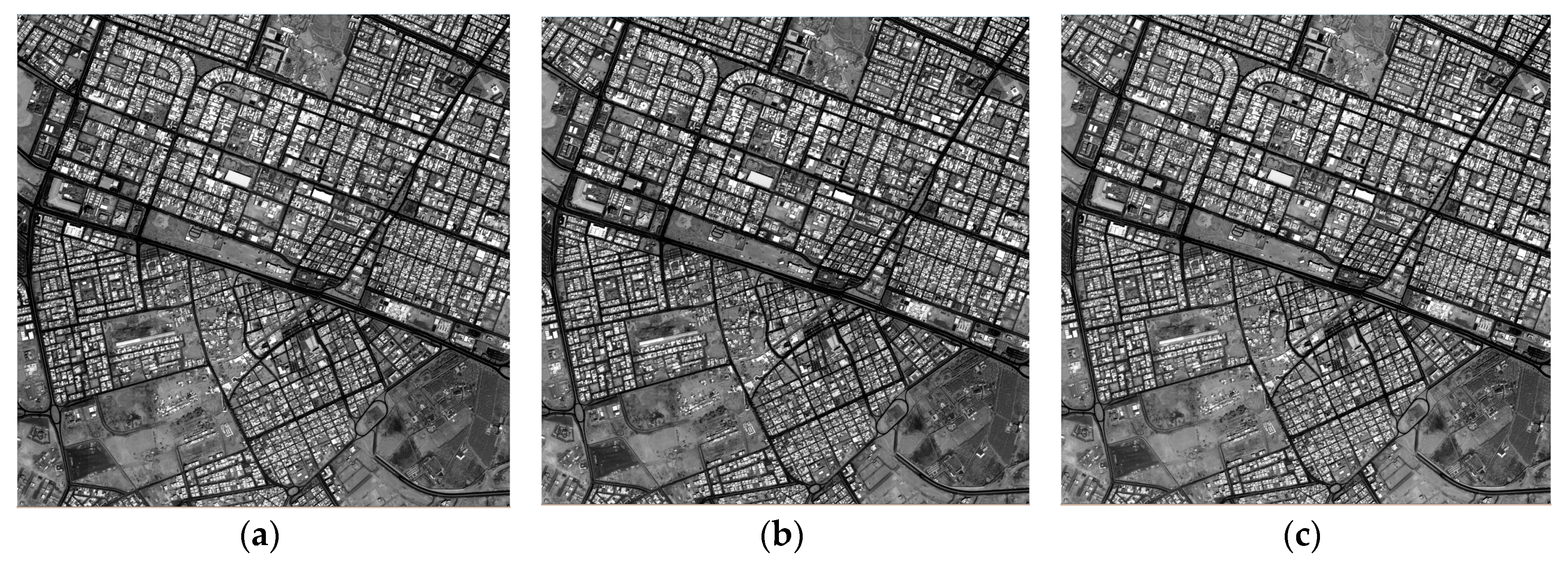
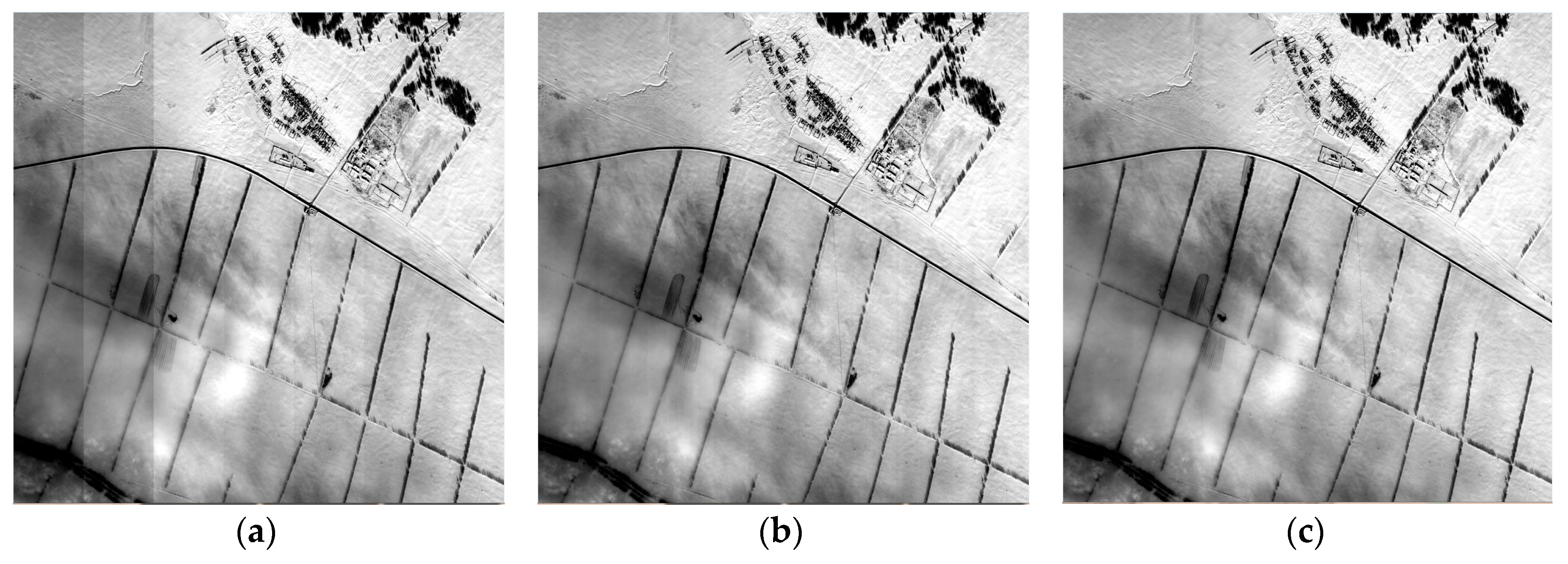
4.4. Verification Results for Raw Images in Group C
5. Discussion
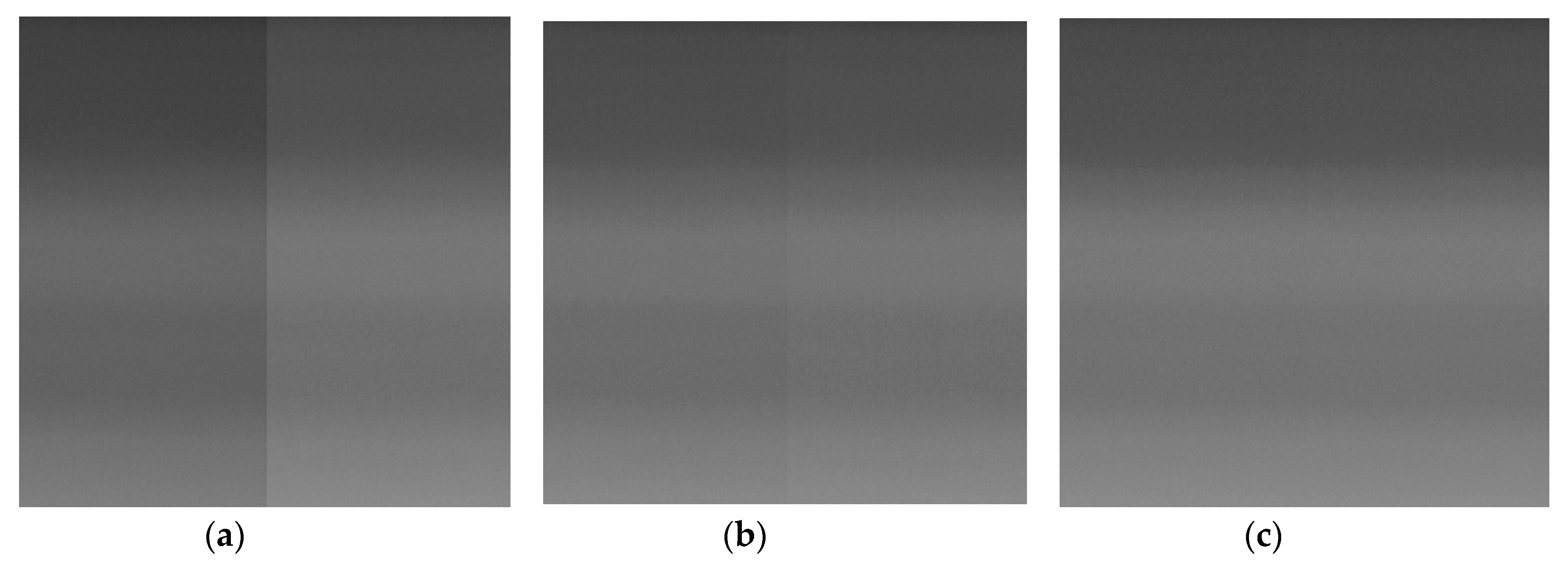
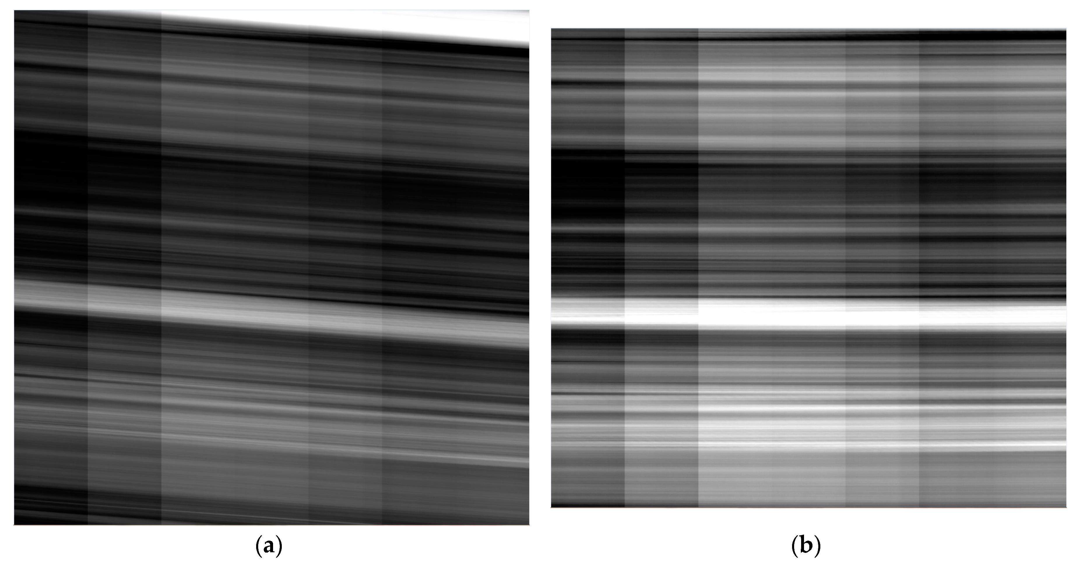
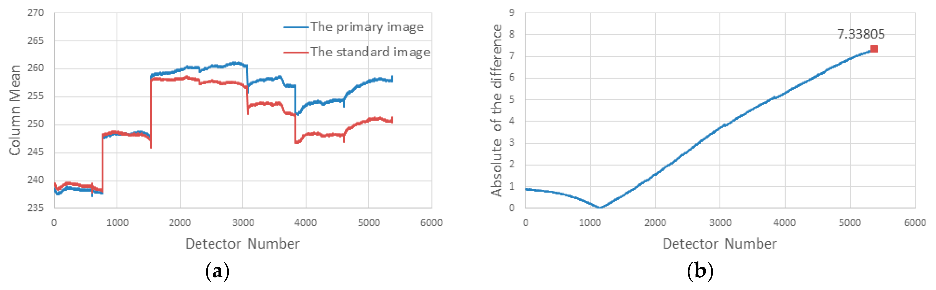
5.1. The Analysis of Pre-Processing
5.2. The Analysis of Corrected Images
6. Conclusions
Acknowledgments
Author Contributions
Conflicts of Interest
References
- Schott, J.R. Remote Sensing: The Image Chain Approach; Oxford University Press on Demand: Oxford, UK, 2007. [Google Scholar]
- Xiong, X.; Barnes, W. An overview of modis radiometric calibration and characterization. Adv. Atmos. Sci. 2006, 23, 69–79. [Google Scholar] [CrossRef]
- Li, Z.; Yu, F. A real time de-striping algorithm for geostationary operational environmental satellite (goes) 15 sounder images. In Proceedings of the 2015 CALCON Technical Meeting, Logan, UT, USA, 26 August 2015. [Google Scholar]
- Zenin, V.A.; Eremeev, V.V.; Kuznetcov, A.E. Algorithms for relative radiometric correction in earth observing systems resource-p and canopus-v. In Proceedings of the ISPRS—International Archives of the Photogrammetry, Remote Sensing and Spatial Information Sciences, Prague, Czech Republic, 12–19 July 2016. [Google Scholar]
- Duan, Y.; Zhang, L.; Yan, L.; Wu, T.; Liu, Y.; Tong, Q. Relative radiometric correction methods for remote sensing images and their applicability analysis. Int. J. Remote Sens. 2014. [Google Scholar] [CrossRef]
- Krause, K.S. Worldview-1 pre and post-launch radiometric calibration and early on-orbit characterization. In Proceedings of the Optical Engineering + Applications, San Diego, CA, USA, 20 August 2008; International Society for Optics and Photonics: Bellingham, WA, USA, 2008; pp. 708111–708116. [Google Scholar]
- Lyon, P.E. An automated de-striping algorithm for ocean colour monitor imagery. Int. J. Remote Sens. 2009, 30, 1493–1502. [Google Scholar] [CrossRef]
- Gadallah, F.L.; Csillag, F.; Smith, E.J.M. Destriping multisensor imagery with moment matching. Int. J. Remote Sens. 2000, 21, 2505–2511. [Google Scholar] [CrossRef]
- Li, H.; Man, Y.-Y. Relative radiometric calibration method based on linear CCD imaging the same region of non-uniform scene. In Proceedings of the International Symposium on Optoelectronic Technology and Application 2014, Beijing, China, 18 November 2014; pp. 929906–929909. [Google Scholar]
- Pesta, F.; Bhatta, S.; Helder, D.; Mishra, N. Radiometric non-uniformity characterization and correction of landsat 8 oli using earth imagery-based techniques. Remote Sens. 2015, 7, 430–446. [Google Scholar] [CrossRef]
- Anderson, C.; Naughton, D.; Brunn, A.; Thiele, M. Radiometric correction of rapideye imagery using the on-orbit side-slither method. In Proceedings of the SPIE Remote Sensing, Prague, Czech Republic, 28 October 2011; International Society for Optics and Photonics: Bellingham, WA, USA, 2011; pp. 818008–818015. [Google Scholar]
- Kubik, P.; Pascal, W. Amethist: A method for equalization thanks to histograms. In Sensors, Systems, and Next-Generation Satellites VIII; Meynart, R., Neeck, S.P., Shimoda, H., Eds.; Spie-Int Soc Optical Engineering: Bellingham, WA, USA, 2004; Volume 5570, pp. 256–267. [Google Scholar]
- Henderson, B.G.; Krause, K.S. Relative radiometric correction of quickbird imagery using the side-slither technique on orbit. In Proceedings of the SPIE 49th Annual Meeting Optical Science and Technology, Denver, CO, USA, 26 October 2004; International Society for Optics and Photonics: Bellingham, WA, USA, 2004; pp. 426–436. [Google Scholar]
- Zhang, G.; Litao, L.I. A study on relative radiometric calibration without calibration field for YG-25. Acta Geod. Cartogr. Sin. 2017, 46, 1009–1016. [Google Scholar]
- Peng, Y.; Huang, H.-L.; Zhu, L.-M. The in-orbit resolution detection of TH-01 CCD cameras based on the radial target. Geomat. Spat. Inf. Technol. 2013, 7, 47. [Google Scholar]
- Gerace, A.; Schott, J.; Gartley, M.; Montanaro, M. An analysis of the side slither on-orbit calibration technique using the dirsig model. Remote Sens. 2014, 6, 10523–10545. [Google Scholar] [CrossRef]
- Otsu, N. A threshold selection method from gray-level histograms. IEEE Trans. Syst. Man. Cybern. 1979, 9, 62–66. [Google Scholar] [CrossRef]
- Pan, Z.; Gu, X.; Liu, G.; Min, X. Relative radiometric correction of CBERS-01 CCD data based on detector histogram matching. Geomat. Inf. Sci. Wuhan Univ. 2005, 30, 925–927. [Google Scholar]
- Spontón, H.; Cardelino, J. A review of classic edge detectors. Image Process. Line 2015, 5, 90–123. [Google Scholar] [CrossRef]
- Horn, B.K.; Woodham, R.J. Destriping landsat mss images by histogram modification. Comput. Graph. Image Process. 1979, 10, 69–83. [Google Scholar] [CrossRef]
- Tong, X.; Xu, Y.; Ye, Z.; Liu, S.; Tang, X.; Li, L.; Xie, H.; Xie, J. Attitude oscillation detection of the ZY-3 satellite by using multispectral parallax images. IEEE Trans. Geosci. Remote Sens. 2015, 53, 3522–3534. [Google Scholar] [CrossRef]
- Chen, S.; Yang, B.; Wang, H. Design and Experiment of the Space Camera; Aerospace Publishing Company: London, UK, 2003. [Google Scholar]
- Yufeng, H.Y.Z. Analysis of relative radiometric calibration accuracy of space camera. Spacecr. Recovery Remote Sens. 2007, 4, 12. [Google Scholar]
- Krause, K.S. Relative radiometric characterization and performance of the quickbird high-resolution commercial imaging satellite. In Proceedings of the SPIE 49th Annual Meeting Optical Science and Technology, Denver, CO, USA, 26 October 2004; International Society for Optics and Photonics: Bellingham, WA, USA, 2004; pp. 35–44. [Google Scholar]
- Krause, K.S. Quickbird relative radiometric performance and on-orbit long term trending. In Proceedings of the SPIE Optics + Photonics, San Diego, CA, USA, 7 September 2006; International Society for Optics and Photonics: Bellingham, WA, USA, 2006; pp. 62912P–62960P. [Google Scholar] [CrossRef]
- Chen, J.; Shao, Y.; Guo, H.; Wang, W.; Zhu, B. Destriping cmodis data by power filtering. IEEE Trans. Geosci. Remote Sens. 2003, 41, 2119–2124. [Google Scholar] [CrossRef]
- Corsini, G.; Diani, M.; Walzel, T. Striping removal in MOS-B data. IEEE Trans. Geosci. Remote Sens. 2000, 38, 1439–1446. [Google Scholar] [CrossRef]
- Ndajah, P.; Kikuchi, H.; Yukawa, M.; Watanabe, H.; Muramatsu, S. SSIM image quality metric for denoised images. In Proceedings of the 3rd WSEAS Internayional Conference on Visualization, Imaging and Simulation, Faro, Portugal, 3–5 November 2010; pp. 53–58. [Google Scholar]


| Group Name | Data Type | Imaging Time | TDI Level |
|---|---|---|---|
| Group A | Side-slither data (Calibration data) | 16 October 2015 | 48 |
| Group B | Side-slither data (Verification data) | 29 October 2015 | 48 |
| Group C | Water (Verification data) | 02 October 2015 | 32 |
| City (Verification data) | 02 October 2015 | 32 | |
| Desert (Verification data) | 10 October 2015 | 48 |
| Correction Method | Mean Value | Standard Deviation | RA (%) | RE (%) | The Maximum Streaking Metrics |
|---|---|---|---|---|---|
| Standard data | 565.7841 | 146.0522 | 22.4864 | 1.6745 | 2.5835 |
| On-orbit coef | 564.7518 | 145.5909 | 0.2657 | 0.1751 | 0.3456 |
| Side-slither coef | 564.8308 | 145.6084 | 0.0082 | 0.0335 | 0.0145 |
| Correction Method | Mean Value | Standard Deviation | Improved Factor (IF) | SSIM | The maximum Streaking Metrics |
|---|---|---|---|---|---|
| Raw data | 75.9497 | 9.6081 | / | / | 4.1526 |
| On-orbit coef | 75.9763 | 8.9793 | 17.2223 | 0.9983 | 1.4877 |
| Side-slither coef | 83.5691 | 10.6944 | 22.6357 | 0.9923 | 0.8967 |
| Correction Method | Mean Value | Standard Deviation | Improved Factor (IF) | SSIM | The Maximum Streaking Metrics |
|---|---|---|---|---|---|
| Raw data | 289.1120 | 73.6728 | / | / | 2.0004 |
| On-orbit coef | 288.0641 | 73.1624 | 5.4147 | 0.9996 | 0.7410 |
| Side-slither coef | 313.7601 | 75.2528 | 15.0459 | 0.9938 | 0.5275 |
| Correction Method | Mean Value | Standard Deviation | Improved Factor (IF) | SSIM | The Maximum Streaking Metrics |
|---|---|---|---|---|---|
| Raw data | 667.4973 | 62.28675 | / | / | 2.5343 |
| On-orbit coef | 668.104 | 60.1704 | 1.7096 | 0.9975 | 1.4192 |
| Side-slither coef | 666.4261 | 59.4314 | 10.4055 | 0.9995 | 0.3067 |
© 2018 by the authors. Licensee MDPI, Basel, Switzerland. This article is an open access article distributed under the terms and conditions of the Creative Commons Attribution (CC BY) license (http://creativecommons.org/licenses/by/4.0/).
Share and Cite
Wang, M.; Chen, C.; Pan, J.; Zhu, Y.; Chang, X. A Relative Radiometric Calibration Method Based on the Histogram of Side-Slither Data for High-Resolution Optical Satellite Imagery. Remote Sens. 2018, 10, 381. https://doi.org/10.3390/rs10030381
Wang M, Chen C, Pan J, Zhu Y, Chang X. A Relative Radiometric Calibration Method Based on the Histogram of Side-Slither Data for High-Resolution Optical Satellite Imagery. Remote Sensing. 2018; 10(3):381. https://doi.org/10.3390/rs10030381
Chicago/Turabian StyleWang, Mi, Chaochao Chen, Jun Pan, Ying Zhu, and Xueli Chang. 2018. "A Relative Radiometric Calibration Method Based on the Histogram of Side-Slither Data for High-Resolution Optical Satellite Imagery" Remote Sensing 10, no. 3: 381. https://doi.org/10.3390/rs10030381