Satellite Rainfall (TRMM 3B42-V7) Performance Assessment and Adjustment over Pahang River Basin, Malaysia


1
Department of Civil Engineering, Faculty of Engineering, Universiti Putra Malaysia, 43400 Serdang, Malaysia
2
Department of Agriculture Technology, Faculty of Agriculture, Universiti Putra Malaysia, 43400 Serdang, Malaysia
*
Author to whom correspondence should be addressed.
Remote Sens. 2018, 10(3), 388; https://doi.org/10.3390/rs10030388
Submission received: 26 December 2017
/
Revised: 22 February 2018
/
Accepted: 23 February 2018
/
Published: 2 March 2018
Abstract
:The Tropical Rainfall Measuring Mission (TRMM) was the first Earth Science mission dedicated to studying tropical and subtropical rainfall. Up until now, there is still limited knowledge on the accuracy of the version 7 research product TRMM 3B42-V7 despite having the advantage of a high temporal resolution and large spatial coverage over oceans and land. This is particularly the case in tropical regions in Asia. The objective of this study is therefore to analyze the performance of rainfall estimation from TRMM 3B42-V7 (henceforth TRMM) using rain gauge data in Malaysia, specifically from the Pahang river basin as a case study, and using a set of performance indicators/scores. The results suggest that the altitude of the region affects the performances of the scores. Root Mean Squared Error (RMSE) is lower mostly at a higher altitude and mid-altitude. The correlation coefficient (CC) generally shows a positive but weak relationship between the rain gauge measurements and TRMM (0 < CC < 0.4), while the Nash-Sutcliffe Efficiency (NSE) scores are low (NSE < 0.1). The Percent Bias (PBIAS) shows that TRMM tends to overestimate the rainfall measurement by 26.95% on average. The Probability of Detection (POD) and Threat Score (TS) demonstrate that more than half of the pixel-point pairs have values smaller than 0.7. However, the Probability of False Detection (POFD) and False Alarm Rate (FAR) show that most of the pixel-point gauges have values lower than 0.55. The seasonal analysis shows that TRMM overestimates during the wet season and underestimates during the dry season. The bias adjustment shows that Mean Bias Correction (MBC) improved the scores better than Double-Kernel Residual Smoothing (DS) and Residual Inverse Distance Weighting (RIDW). The large errors imply that TRMM may not be suitable for applications in environmental, water resources, and ecological studies without prior correction.
1. Introduction
For many environmental, water resources, and ecological applications, it is important to quantify rainfall accurately. However, quantifying the rainfall can be challenging, especially in inaccessible areas such as Antarctica and Amazonia. The Tropical Rainfall Measuring Mission (TRMM) is a research satellite designed to provide information on rainfall in the tropical and sub-tropical regions of the Earth. The TRMM Multi-Satellite Precipitation Analysis (TMPA), also known as TRMM 3B42, is an algorithm that provides the best estimation of rainfall based on a combination of measurements from multiple sensors onboard multiple satellites [1]. TRMM 3B42 provides rainfall values between 1998 and 2014 and presents one of the most valuable 17 years of spatiotemporal rainfall datasets to date.
The algorithm of TRMM Multisatellite Precipitation Analysis involves data sources from multiple other satellites which are precipitation-related passive microwave and infrared measurements [1]. These are inter-calibrated and merged with the sensor measurements onboard the TRMM satellite, followed by gauge-adjustment at the monthly timescale before back-scaling to a three hourly temporal resolution. The multiple data sources and multiple levels of processing result in many sources of errors in the final product. There have been efforts to evaluate TRMM rainfall data, but until now, there is still limited knowledge of the accuracy of the TRMM 3B42 in its latest version 7 (henceforth TRMM for brevity) over the tropical regions of Asia, which restricts its application in the field of ecology, climate, and hydrology [2]. Topography, seasonality, and climatology have been shown to play a role in the satellite precipitation products performance.
Topography affects the TRMM rainfall performances, especially in terms of detection probability and bias. In Thailand, regions with complex terrain exhibited poor rain detection and magnitude-dependent mean errors [3]. In Morocco, TRMM can estimate precipitation events at elevations below 1000 m accurately, but faces difficulties within the area of high elevations with high snow content and low rainfall [4]. The signals in the microwave region could be scattered due to the cold areas (or snow-covered areas) and complex terrain region [1]. This may be attributed to the TRMM Microwave Imager (TMI) onboard the TRMM satellite. TMI is sensitive to the temperature and as a consequence, it can lead to inaccurate rainfall rates. A study carried in Northeastern Iberia showed TRMM to exhibit a good performance in regions with minimum precipitation events and a low altitude, and shows a poor performance on the coastal areas and in complex terrains [5]. The impacts of altitude on the TRMM accuracy are consistent with a study carried out by Ouatiki et al. (2017) in Morocco that showed that the TRMM product had problems in estimating rainfall rates over mountainous regions [6]. The difficulties are due to the ability of a Precipitation Radar (PR) to obtain the information about the rain event such as the intensity and distribution, the rain type, and other data [7]. The mountainous region may shield the radar beam to obtain such information. It also can be caused by the radar wave that hits the ground, returning false echoes [8].
In addition, the temporal and spatial scale also affects the performance of TRMM estimates. There are some uncertainties which makes the sensitivity of local-scale rainfall in a small region contentious [9]. These include the lack of TRMM precipitation algorithm sensitivity to low and high precipitation clouds [10,11], the effect of upscaling the rainfall rate to an effective temporal scale [12], and the coarse grid size of the TRMM data for solving local rainfall patterns [13].
The TRMM rainfall performances are also found to be affected by the climatology of a region. Areas with high snow content are problematic due to the sensitivity to the surface emissivity in passive microwave sensors, which produces signals similar to those of precipitation [13]. Satellite-based precipitation datasets also show different performances in warm and cold seasons [14]. Complex emissivity from a cold place and area covered in ice, especially in winter, may be recognized as a rain event, which could lead to missed precipitation by TRMM sensors [15].
Apart from topography and climatology, seasonality also plays a big role in the TRMM rainfall performances. TRMM is reported to be affected by monsoon systems. A study carried out in Malaysia shows that TRMM is less sensitive towards low precipitation clouds than heavy precipitation clouds and the correlation obtained was better during the northeast monsoon [9]. The heaviest rainfall events occurred during the northeast monsoon and were mainly caused by the large-scale monsoon flows that contained heavy precipitation cloud [10]. The error can be explained by the presence of low versus heavy precipitation clouds in wet and dry seasons. Based on the study carried out in Bali, most high-rainfall events increase during the wet season, (December–January–February) and the lowest rainfall events occur during the dry season (June–July–August) [16]. Those conditions are associated and generated with the northeast and southwest monsoon patterns. They found that the correlation levels between rain gauges and TRMM during the wet season are lower, whereas in the dry season, they are a bit higher. As was found in a study carried in China, TRMM can be overestimated and underestimated in both the dry season and wet season, depending on the different rain rates [17]. TRMM under-detects and underestimated rainfall rates during high precipitation events, whereas it over detects and overestimated rainfall rates during light precipitation events [17,18]. Meanwhile, a study carried out in Qinghai Lake Basin, China, shows that TRMM exhibits a poor performance between May and September, which is the dry season [19]. This is consistent with a study carried out in Morocco, which showed that July and August exhibit the lowest correlation coefficients [6]. A study in Circum-Bohai-Sea region, China, showed that the rainfall pattern is more effectively captured by TRMM for the wet region or season than for the dry region or season [20]. In short, the performances of TRMM rainfall can be dependent on season. In the case of Malaysia, the performance may differ depending on the monsoons that take place, which are the northeast monsoon (dry season) and southwest monsoon (wet season).
Rainfall information from a large number of rain gauges is already adopted as part of global satellite algorithms, including TRMM at a final stage of monthly bias correction [1]. A practical method of estimating rainfall can be created by merging the satellite data and rain gauge data. Both satellite and rain gauge data can be merged by combining accurate quantitative rainfall from stations with spatially continuous information from remote sensing observations. Even so, most of the developing countries have a restricted accessibility to rain gauge data. Due to this, the global precipitation product may be found to be unsatisfactory and requiring local adjustment. To improve the performance of satellite algorithms, multiple statistical methods have been proposed. Example statistical methods, many with applications originating from ground-based weather radars, are mean bias correction (MBC) [21,22], double-kernel smoothing (DS) [23], and residual inverse error weighting (RIDW) [24].
On February 2014, the Global Precipitation Mission (GPM) was launched as a follow-on to TRMM and the objective was to observe global precipitation more frequently and more accurately than TRMM. The GPM design is based on improvement of the shortcomings of TRMM and hence an in-depth study of the performance of TRMM could provide the basis for a study on GPM improvements. Yet, despite having a significant period of rainfall records, extensive studies of TRMM accuracy in measuring rainfall in South East Asia, specifically in Malaysia, are sparse. Thus, the objectives of this paper are: (1) to analyse the performance of rainfall estimation from TRMM in Malaysia using the Pahang river basin as a case study; and (2) to compare several adjustment methods for correcting TRMM based on rainfall estimates from ground stations. Pahang river is the largest river in Peninsular Malaysia and the river basin is one of the important water catchment areas in Malaysia that also provides water resources to neighbouring urbanized states such as Selangor. The performance will be assessed by computing a set of performance indicators using rain gauge data. Section 2 will describe the study area, methodology, and datasets used, while Section 3 will present the results and discussion. Finally, Section 4 will provide some conclusions and recommendations for future work.
2. Methods and Data
2.1. Study Area
The location of study is in Pahang. Pahang is situated on 2°25′55″–4°48′4″N and 101°19′18″–104°14′31″E in the Peninsular Malaysia. As shown in Figure 1, the topography of Peninsular Malaysia is dominated by a mountain range known as Banjaran Titiwangsa (Main Range), which extends from the Thailand border southwards to Negeri Sembilan. The largest basin in peninsular Malaysia is the Sg. Pahang Basin [25]. The Sg. Pahang basin has an annual rainfall of about 2170 mm, a large proportion of which occurs during the North-East Monsoon between mid-October and mid-January [26].
Malaysia’s climate is hot and humid throughout the year since it is situated near the equator. The rainfall distribution patterns are dependent on the seasonal wind flow patterns and the local topography features [27]. In particular, Malaysia deals with two distinct monsoons that are the northeast monsoon which blows a wet season from October to March and the Southwest monsoon which blows a dry season from June to September. Throughout the northeast monsoon season, areas such as the east coast of peninsular Malaysia, Western Sarawak, and the northeast coast of Sabah will experience heavy rain spells. In addition, the inland areas or areas which are sheltered by mountain ranges are protected from its influences. In addition, the two shorter periods of inter-monsoon seasons are marked by heavy rainfall as it yields uniform periodic changes in the wind flow patterns over the country.
2.2. Rainfall Data
The TRMM 3B42-V7 dataset was obtained from https://pmm.nasa.gov/data-access/downloads/trmm. The satellite estimates were obtained with a 3-h temporal resolution and 0.25° × 0.25° (approximately 27.8 km × 27.8 km) spatial resolution. The data is extracted for the region covering Pahang (latitudes and longitude boundaries) and for the years 1998–2014 (17 years). In order to match the temporal resolution of the rain gauge data, which is daily, the values were aggregated to the daily scale. The three-hourly rainfall rate was assumed to be constant over the 3 h, and the all the three-hourly total rainfalls in the defined 24-h period are summed to get the total daily rainfall.
Meanwhile, the ground-based (rain gauge) rainfall data are obtained from Department of Irrigation and Drainage (DID). The data are taken from all 32 stations in Pahang with data on record between 1998 and 2014. Table A1 (Appendix A) shows the rain gauge stations which were collocated with the midpoints of TRMM pixels. As several TRMM pixels contained more than one station within the pixel, this resulted in a total of 27 pixel—point pairs. For these pixels, the rain gauge values from the multiple stations were averaged to obtain a pixel-averaged time series.
The study region is further divided into the low-altitude (h < 100 m), mid-altitude (100 m < h < 500 m), and high-altitude (h > 500 m) areas using the Digital Elevation Model from the Shuttle Radar Topography Mission (SRTM) Version 3.0 Global 1 arc second Data (data available from the U.S. Geological Survey). Table 1 shows the number of pixel-point pairs based on the altitudes. It is important to note that satellite-derived measurements are different from ground station observations for various reasons. The satellite sensors have finite field-of-views, thus when a measurement is taken by a satellite sensor, it represents the average value within a pixel. Besides that, measurements from ground stations are generally point values. Therefore, satellite measurements are intrinsically different from ground station measurements.
2.3. Performance of Precipitation Estimations Analysis
2.3.1. Detection Metrics
Rainfall detection metrics are the performance criteria that compare the occurrence and non-occurrence of rainfall events between TRMM and rain gauges. Table 2 shows the detection metrics used in this study.
2.3.2. Volumetric Metrics
The satellite product and rain gauge time series were compared to analyse their variation and relationship using various volumetric metrics: Root Mean Squared Error (RMSE), Correlation Coefficient (CC), Nash-Sutcliffe Efficiency (NSE), and Percent Bias (PBIAS). Table 4 shows the standard verification indices for evaluating the TRMM rainfall data.
2.4. Bias Adjustment Parameters
The evaluation of each point value is carried out using a cross validation against the rain gauge observations for examining the improvement in the accuracy of the satellite rainfall estimates. In this study, leave-one-out cross validation was used to evaluate the three adjustment methods for all events using the performance indicators. Leave-one-out cross validation was used such that one rainfall data is removed at a time from the data set and the value is estimated from the remaining data [30].
2.4.1. Mean Bias Correction (MBC)
The mean bias correction (MBC) provides information on the long-term performance of the correlations by allowing a comparison of the actual deviation between calculated and measured values term by term. MBC is the simplest method in which a bias correction factor is constant over time and space [31,32,33]. The MBC factor is calculated for each time step as an average across all point-pixel pairs and is multiplied with the satellite estimates over the entire study area. For each time step, the correction factor can be calculated as follows:
where, N = the number of available gauges inside the satellite domain, and = the gauge and satellite daily rainfall values corresponding to gauged location j.
2.4.2. Residual Inverse Distance Weighting (RIDW)
The method estimates the unknown value at one point using a linearly weighted combination of its neighbour sample points, with the weights inversely related to the distance between the estimated and sample point [34]. The bias adjustment is based on a previous study carried in Ethiopia [35]. First of all, the satellite rainfall estimates are extracted at rain gauge locations. The differences between satellite and rain gauge estimates are calculated at each station location. These residuals are interpolated using inverse distance weighting (IDW) to each satellite pixel centre and the interpolated differences are added back on to the satellite estimates. The weights for each sample are inversely proportional to the distance from the point being estimated:
where, Px = estimate of rainfall for the ungauged station, = the gauge and satellite daily rainfall values corresponding to gauged location j, dj = distance from each location the point being estimated, N = No. of surrounding stations.
2.4.3. Double-Kernel Residual Smoothing (DS)
The double-kernel smoothing technique (DS) is used to estimate the residual field by a weighted average of point residuals , using kernel functions, and then adjust the satellite field by the predicted residual field [23]. The point residual at the given gauged location j = 1, …, N is defined as:
where and = the gauge and satellite daily rainfall values corresponding to gauged location j.
The idea of a double smoothing estimator is by adding new pseudo observations by a coarse interpolation and leading to the production of the final estimates. There are two steps that need to be taken for the double smoothing estimator to be constructed. Firstly, the original residual is transformed to a gridded pseudoresidual with equal spacing. At the given gridpoint location i = 1, …, M, the pseudoresidual is defined to be:
where ||.|| is the Euclidean norm and is the Kernel function defined as a Gaussian kernel following Li and Shao [23]:
The variable H is the position of the points, and the bandwidth b is determined using Silverman’s rule of thumb:
where, n = number of samples and s is the standard deviation of samples.
The second step of DS is applied to both the residuals and pseudoresiduals to estimate the final error field
The merged product ZDS at point k is calculated by subtracting the corresponding error from the satellite estimate ZSk:
The kernel smoothing (interpolation) of the residuals does not rely on the stationary assumption. Thus, the product of the merging will converge toward the rain gauge estimates with decreased distance toward the ground observations.
3. Results and Discussion
3.1. Comparison between Satellite Product and the Rain Gauge Data
3.1.1. Detection Metrics
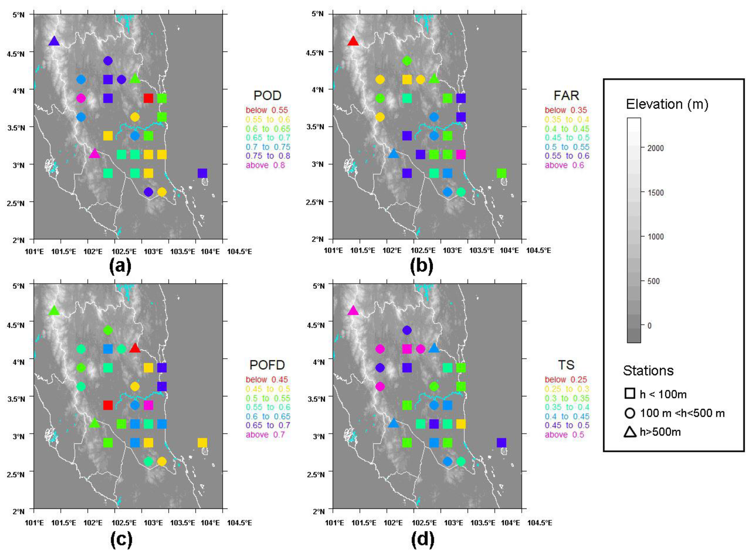
The probability of detection (POD) values for rainfall estimates in Pahang are shown in Figure 2a. The figure shows that 14 out of 27 pixel-point pairs located in the low and mid-altitude region have POD scores lower than 0.7. The lowest POD value is 0.54, which is located near to the coast. Table 5 shows that the POD values vary from 0.5 to 0.8 (with average POD of 0.68), which can be considered as an acceptable performance. A previous study analysing the performance of TRMM, amongst other satellite products over a smaller time window (2003–2007), shows that the POD for the rain gauges in Pahang have a range of 0.7–0.8, which is close to the range of scores obtained (0.5–0.8) [36]. The region-specific performance could be due to the fact that the spatial resolution (0.25°) causes TRMM estimates to be insensitive to local-scale precipitation events.
Figure 2b shows the False Alarm Ratio (FAR) of the rainfall estimates in Pahang Basin. The lowest FAR value is located at the Gunung Brinchang station (4.625°N, 101.375°E), which is 0.32. The highest FAR value is 0.62, which is located near to the east coast of Pahang. There are 14 out of 27 pixel-point gauges located in the low and mid-altitude region that have FAR scores of more than 0.45 This result is consistent with the study carried out in Nepal, which shows a higher FAR in a low elevation region [37]. Table 5 shows that FAR values vary from 0.3 to 0.5.
Figure 2c shows the Probability of False Detection (POFD) for rainfall estimates in Pahang Basin. The POFD scores across the study area appear to be independent of geographical characteristics. The independency can be explained by the sensitivity of microwave and infrared retrieval algorithms to scattering signals and cold cloud temperatures from the rainfall systems over these terrain features [38]. The majority of the pixel-point gauges located at the coast have a POFD value of more than 0.6, indicating a tendency of TRMM to over detect rainfall. Table 5 shows the POFD values at each pixel-point pair.
Figure 2d shows the TS of TRMM in Pahang. The highest TS value is in Gunung Brinchang (4.625°N, 101.375°E), with TS = 0.57. There are 17 out of 27 pixel-point pairs that have TS scores lower than 0.5. The figure shows that the overall TS is poor despite having the highest value of 0.57. On the east coast, it shows that the majority of the pixel-point pairs have TS scores lower than 0.4.
3.1.2. Volumetric Metrics
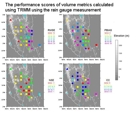
Figure 3a–d show the performances of the TRMM daily product in terms of RMSE, PBIAS, NSE, and CC. Table 6 shows the performance scores calculated using TRMM using the rain gauge measurement.
Figure 3a shows the RMSE between the gauge and TRMM daily rainfall over the Pahang Basin. The lowest RMSE is found in one of the high-altitude stations (RMSE = 12.80 mm/day) at Gunung Brinchang Station. However, the value is still considered as a large error, considering the average daily rainfall at the station is 19.14 mm/day. On the other hand, the higher RMSE is located near to the coastal region (RMSE = 29.87 mm/day). This result agrees with a study in Iran, which shows that estimations of satellite rainfall in highland and mountainous areas are more accurate than in lowland areas [39]. Besides that, TRMM performs poorly on coastal and island sites, which is consistent with the study carried out in Tropical Pacific Basin [40]. The convergence zones can be persistent when the breezes and synoptic gradient winds interact with each other and the surface friction increases in transition from sea to land [41]. When the level of convergence of moist air is low, it will assist the dynamical and microphysical processes for the formation of clouds and precipitation [41]. Due to this, the TRMM estimates can be inaccurately measured.
Figure 3b shows the percent bias (PBIAS) for Pahang. The positive or negative values indicate overestimation or underestimation bias, respectively. Most of the PBIAS values that are close to zero and negative are in the east coast of Pahang. This is consistent with a previous study which also showed that TRMM underestimates rainfall in the coast [36]. These are also the same pixel-point pairs associated with high RMSE values. During the northeast monsoon season, the exposed areas like the east coast of Peninsular Malaysia experience heavy rain spells. Underestimation in satellite-based precipitation products may be caused by the heavy rainfall which can cause a reduction in the signal of the passive microwave (PMW) sensor [42]. Usually on the coastal area, the frequent occurrence of low stratiform clouds can affect the TRMM estimates if the clouds are under stable conditions, which is detached from precipitation patterns [43]. The average PBIAS value is 26.95%, which indicates an overall overestimation bias.
Figure 3c shows the Nash Sutcliffe Efficiency (NSE) of rainfall estimates in Pahang Basin. Efficiency scores below 0 indicates that the TRMM rainfall results are less accurate than the mean of the observed data and therefore very poor estimates [44]. The figure shows that most of the values are under 0, and the NSE values reduced as the area moved further away from the coast. There is only one station with a positive value (NSE = 0.1), which is located at Pulau Tioman (2.875°N, 104.125°E). Even though the value is positive, it is still low, indicating the weak performance of the satellite product at the daily scale.
Figure 3d shows the correlation coefficient (CC) of rainfall estimates in Pahang basin. The correlation coefficients are shown in Table 6 where the correlations vary from 0 to 0.49. Most of the CC values are positive; however, the average CC value is 0.26, indicating a weak performance. There are 16 out of 27 pixel-point pairs that have CC scores ranging from 0.30 to 0.49. A study in Malaysia also displayed the same range of CC scores in the Pahang area [36].
3.2. Rainfall Performance at Different Elevation Regions
3.2.1. Detection Metrics
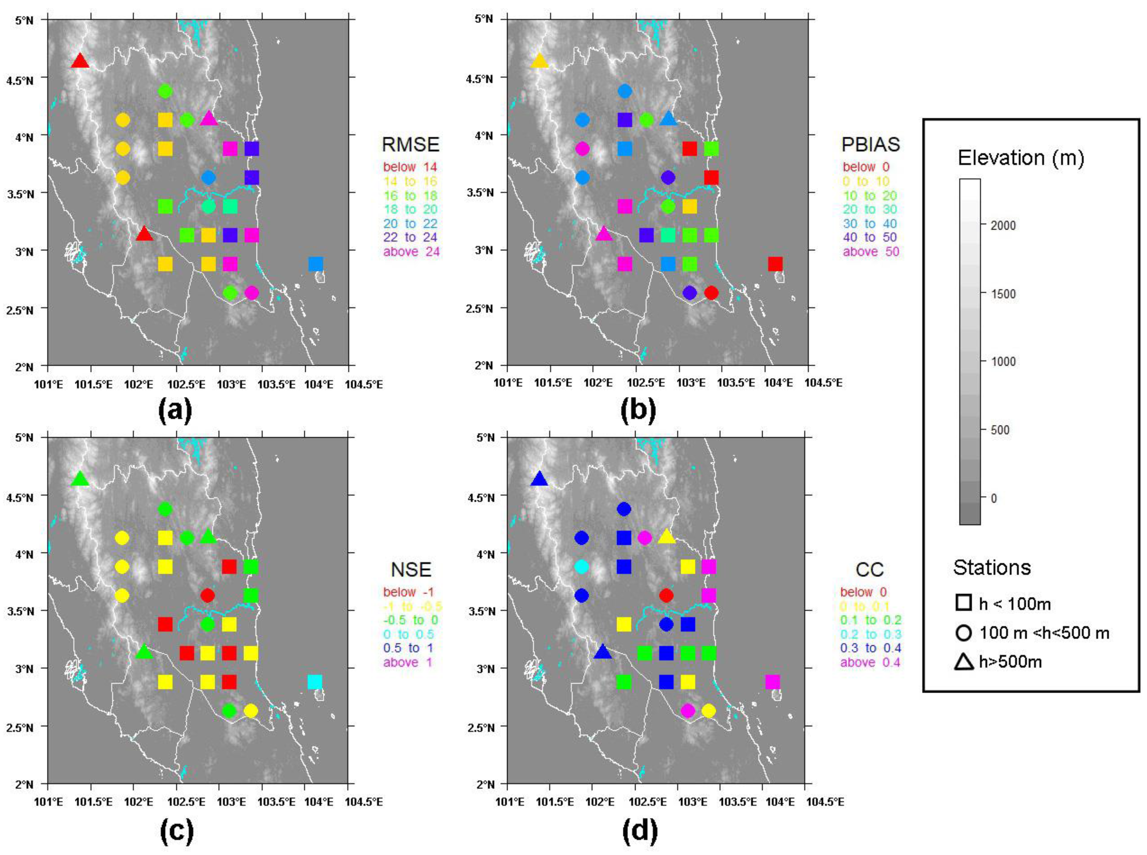
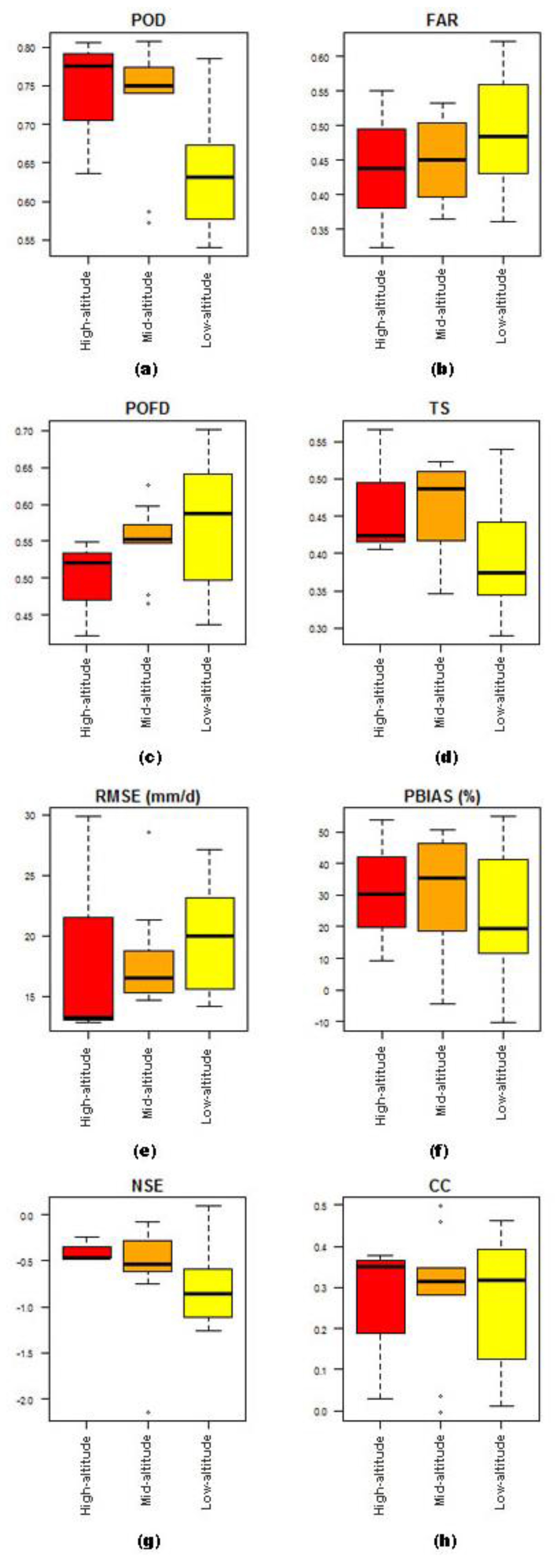
In Figure 4a, approximately 50% of the points in the high-altitude have POD scores higher than 0.77, but the results constitute a higher frequency of lower valued scores. While at the mid-altitude, about 75% of the pixel-point pairs have POD scores of more than 0.74. However, there are exactly two pixel-point pairs that have POD scores below 0.60. In the low-altitude regions, the distribution is positively skewed and all the station scores are under 0.80. There are about 50% pixel-point pairs with POD scores lower than 0.63.
For the FAR scores, Figure 4b shows that the minimum scores are located in the high-altitude region (FAR = 0.32), while the highest scores are located in the low-altitude region (FAR = 0.62). Unlike in the low-altitude region, the high-altitude and mid-altitude region scores distributions are almost symmetrical. Predominantly, the interquartile range is large, indicating that there is a large variability in the results between the pixel-point pairs.
Figure 4c shows the performances of POFD. In the high-altitude region, the highest score in the high-altitude region is 0.54 and the lowest score is 0.44. The lowest score in the high-altitude area also represents the lowest scores in all regions. Almost all pixel-point pairs in the mid-altitude region have scores higher than 0.54. In the low-altitude region, the data distribution is negatively skewed, indicating that the data contains a higher frequency of low valued scores.
The TRMM threat score (TS), on the other hand, shows a large variability for each altitude region. The boxplot for the mid-altitude region in Figure 4d shows that the scores distribution is negatively skewed and 75% of the pixel-point pairs have scores lower than 0.49. As for the high-altitude and low-altitude region, the scores distribution is positively skewed, indicating that the data constitute a higher frequency of high valued scores.
3.2.2. Volumetric Metrics
For the RMSE in Figure 4e, the scores for the high-altitude region and low-altitude region have a large variability since the interquartile range for both altitudes is respectively large. Overall, the highest RMSE score and the lowest RMSE score are located in the high-altitude region. The mid-altitude region has the smallest variability in scores compared to other regions. Station Sg. Anak Endau Kg. Mok in the mid-altitude region have a high score compared to the other station and are numerically far from other scores (RMSE = 28.56 mm/day). The results conclude that pixel-point pairs in the mid-altitude region have overall good RMSE performances compared to other regions.
In Figure 4f, the PBIAS scores distribution in the mid-altitude area are negatively skewed; about half of the pixel-point pairs in the region have scores below 35.6%. Compared to the mid-altitude region, the scores distribution in the low-altitude region is positively skewed, where the scores constitute a higher frequency of high PBIAS. In the high-altitude region, the score distribution is normal.
The highest NSE score is 0.09, which is located in the low-altitude region. In Figure 4g, the TRMM scores distribution in the low-altitude region is positively skewed. This indicates that the scores constitute s higher frequency of higher NSEs. Similarly, the TRMM scores distributions in the mid-altitude and high-altitude region are also positively skewed. The overall NSE performances were poor, as generally, all pixel-point pairs in the high- and mid-altitude areas had NSE values below 0 and almost 75% of the pixel-point pairs in the low-altitude area had NSE values below 0.
The CC scores distributions in the high-altitude and low-altitude regions are negatively skewed in Figure 4h. The scores in both regions constitute a higher frequency of lower CC. The overall highest CC score is located in the mid-altitude region (CC = 0.49). Figure 4h concludes that most of the pixel-point pairs at all regions have CC values below 0.4, which indicates poor performances. Compared to other regions, the mid-altitude region shows a slightly better performance as there are two pixel-point pairs with high CC values and the differences in CC values in the mid-altitude region are not too distinct.
3.3. Seasonal Analysis of TRMM
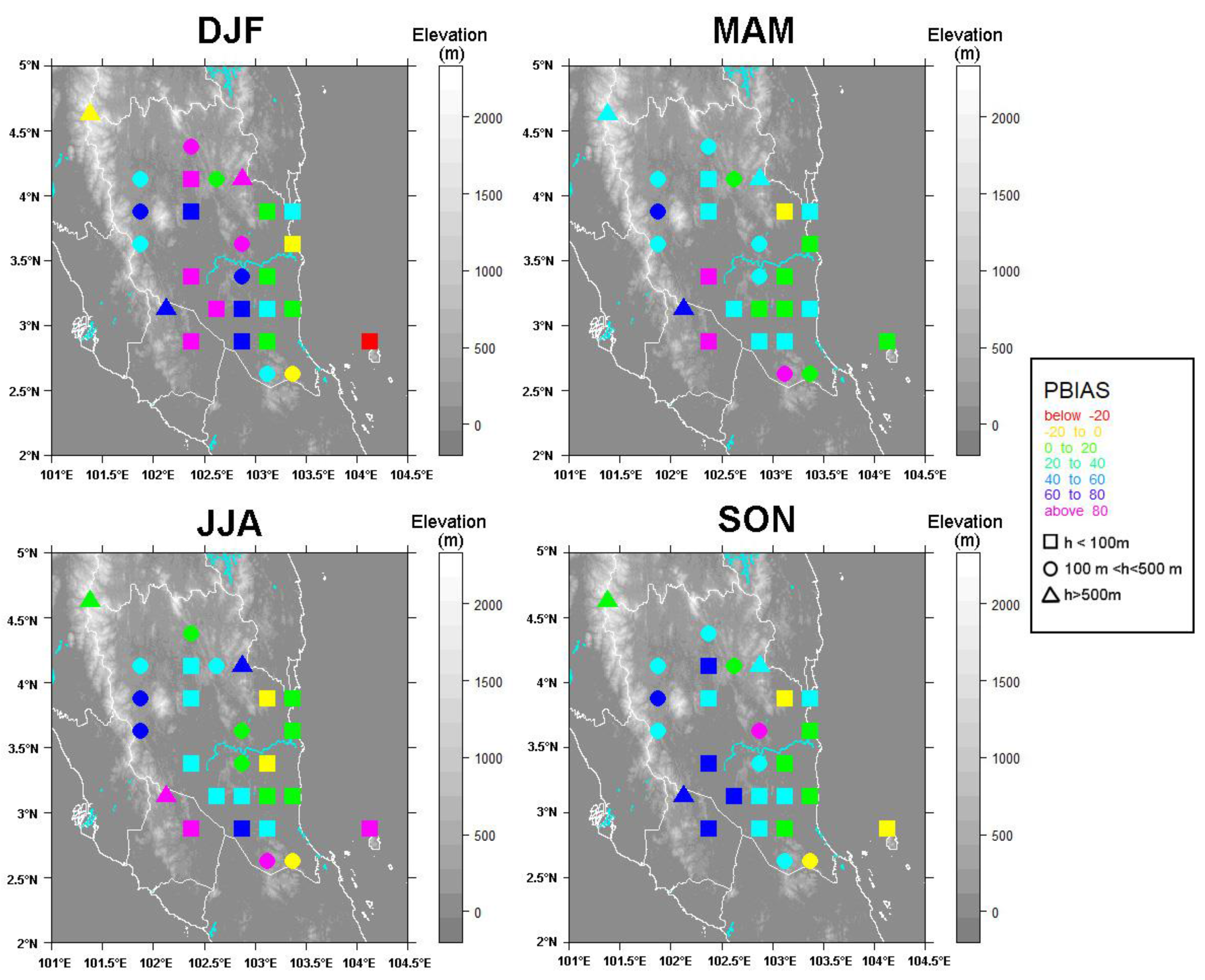
A seasonal analysis is performed by taking all seasons from 1998 to 2014 into consideration. Figure 5 shows the PBIAS of TRMM in each season. During the wetter seasons (DJF and MAM), negative bias occurs in the coastal region and in Cameron Highland (highest altitude pixel-point pair). The rest of the locations show high numbers of overestimated PBIAS readings. This is contrary to other reports of underestimations during the wet season, for example, by Zulkafli in Andean–Amazon River [45]. Inland locations generally show overestimations. DJF and MAM seasons are overestimated on average by 33.05% and 30.33%, respectively. In dry seasons, there are several locations that show an underestimation by TRMM, mostly located in the area close to the coastal region. However, on average, the average PBIAS reading for JJA and SON is 29.81% and 22.92%, respectively, demonstrating overestimation. The overestimation in the wet season and dry season in the inland locations may be attributed to the type of rainfall events that predominantly occur, which are longer term low to moderate intensity rainfall. TRMM can overestimate rain for light and moderate rain rates and underestimate for heavy rain rates, as reported by Guo [17].
3.4. Rainfall Performance After Bias Adjustment
3.4.1. Detection Metrics
Figure 6 shows the performance scores for detection metrics after bias adjustment. In Table 7, the average scores of both pre-corrected and post-corrected TRMM are compared. The average pre-corrected POD shows a moderate performance, but after bias adjustment, the scores improved. POD scores at a high altitude generally show a smaller increase compared to POD scores at mid-altitude and low-altitude.
As for FAR and POFD, the scores reduced towards zero, indicating better detection skills. The MBC method reduces FAR, especially at high altitudes and mid-altitude pixel-point pairs. Compared to the MBC method, the DS method reduces FAR especially for pixel-point pairs in low-altitude and mid-altitude regions. The RIDW method has the highest average FAR and the altitude seems to have no effect on the reduction. For POFD, the MBC method shows that 50% of the pixel-point pairs have scores below 0.2, which indicates a good performance. The majority of the pixel-point pairs located in the low-altitude and mid-altitude region have POFD scores below 0.2 after correction using the DS method. However, the RIDW method shows that only a few of the pixel-point pairs in the coastal and inland regions have POFD scores below 0.3. Half of the pixel-point pairs have scores in the range of 0.3–0.4.
On the other hand, the average pre-corrected TS shows a slightly weak performance, but after being bias adjusted, the scores improved. The MBC method improved the scores especially for pixel-point pairs at the coastal region and some pixel-point pairs in the inland region. The DS method particularly improved some pixel-point pairs in the inland region and there is not much improvement in the TS scores for the RIDW method as the average pre-corrected TS score (TSav = 0.423) is close to the average post-corrected TS score (TSav = 0.552).
The scores show that MBC improved the scores the most compared to the other methods. The results show that MBC and DS have a strong correlation with the elevation, unlike the RIDW method. The average performance scores for RIDW show only a small improvement compared to the pre-corrected average.
3.4.2. Volumetric Metrics
Figure 7 shows the performance scores for detection metrics after bias adjustment. In Table 8, the average scores of both pre-corrected and post-corrected TRMM are compared. The average performances score overall in Pahang shows a poor performance before correction. RMSE scores are significantly reduced after the DS method is applied, with an average of 19.14 mm/day before correction and 15.86 mm/day after bias adjustment. The MBC method also performed well in reducing the RMSE scores. However, the RMSE scores are not consistent with the elevations. This may be caused by the correction factor being applied to the pixel-point pairs. The correction factor applied to the pixel-point pairs was calculated using both ground-based and satellite estimates from different elevation regions. The range of pre-corrected RMSE is 12.80–29.87 mm/day and the range of post-corrected RMSE is 9.95–27.17 mm/day.
Most of the PBIAS values corrected by the MBC method that are closer to 0 are on the east coast of Pahang. During the northeast monsoon season, the exposed areas like the east coast of Peninsular Malaysia experience heavy rain spells. The heavy rainfall may cause signal attenuation of the passive microwave (PMW) sensor, which may cause underestimation in satellite-based precipitation products (Qin et al., 2014). The average PBIAS value before correction is +26.95%, which indicates overestimation bias. After the MBC method (range of −34.1%–47.1%) was applied, there was a significant decrease in the average PBIAS value (PBIAS = 3.904%), which indicates a much smaller amount of overestimation. There are 12 out of 27 pixel-point pairs that underestimate the rainfall event. RIDW and the DS method show that the PBIAS scores decrease but remain positive, which indicates overestimated bias. The majority of pixel-point pairs in RIDW (range of −12.9%–98.8%) and the DS method (range of −18.8%–51.2%) are overestimating the rainfall event. However, compared to the MBC method and DS method, the average of PBIAS after being corrected by RIDW increases, from +26.95% (pre-corrected) to +30.32% (post-corrected).
Before correction, half of the pixel-point pairs have NSE values which are under 0. The NSE values reduced as the area moved further away from the coast. The overall NSE values which have been corrected by using the MBC method increase towards 1, which indicates improvement. Some pixel-point pairs increase beyond 0, which indicates a better estimation. Most of the pixel-point pairs after adjustment have NSE values beyond 0, even though the average for the MBC method is still below 0 (NSE = −0.26). Furthermore, the RIDW method shows that there is only one station which shows an NSE value below −1. The range of pre-corrected NSE scores is −0.21 to 0.09 and the range of post-corrected NSE scores is −1.68 to 0.32.
Prior to correction, most of the pixel-point pairs have a positive CC value. However, the average CC value is 0.26 (range between 0–0.5) and this shows a slightly weak overall performance. The higher correlations are located on the east coast of Pahang and the mountainous areas. Most of the post-corrected CC increases towards the perfect score (CC = 1). The average CC value for the MBC method is 0.31 (range of 0.07–0.52), which is the highest average value, followed by the MBC method (CCav = 0.29, range of 0–0.59) and RIDW (CCav = 0.18, range of 0.01–0.36).
4. Conclusions
Rain gauge data were used to evaluate the TRMM performance over the Pahang River basin covering approximately 48,380 km2. A variety of performance indicators are used to evaluate the rainfall measurements in different ways.
Based on the results, TRMM shows a moderate performance in detection and volumetric correspondence between TRMM and rain gauges. This can be verified by the moderate performance of POD and weak performance of TS at most of the pixel-point pairs. The poor performances of TRMM at the coast reflect the inability of TRMM instruments and algorithms to capture the complex rain formation system on the coast. POFD and FAR demonstrate that the pixel-point pairs generally have high false alarm values (POFD > 0.5 and FAR > 0.5). The errors between the rain gauge and TRMM measurement at most of the pixel-point pairs are high. The high errors were located mostly in the coastal areas and this may due to the coastal convergence zone. At most of the pixel-point locations on the east coast of Pahang, TRMM underestimates the rainfall due to heavy rains which can reduce the signal emission to obtain rain event information. The performance of all pixel-point pairs in Pahang is also characterised by a weak average correlation. The results obtained by this study are also consistent with Tan et al., but with more rain gauges to be considered and a longer temporal scale [36].
Based on the seasonal analysis, TRMM generally shows overestimation in both the wet and dry season. This may be caused by the rainfall rates during each season. Three methods are used in this study to adjust the biases. Overall, it shows that MBC performed better than DS and RIDW. The differences in the post-corrected results are because of the different ways in which each method adjusts the biases. Most of the detection and volumetric scores improved after being adjusted.
Based on the detection scores and volumetric scores, TRMM shows a weak to moderate performance at the daily scale. Therefore, the use of the product for analysis and models in the field of ecology, climate, and hydrology will be limited at this scale. The product may be more suitable at higher temporal aggregation values such as monthly or annual scales. Furthermore, the bias correction results show that the errors between TRMM and rain gauge estimates were reduced by up to 18.38% and the correlation between TRMM and rain gauge estimates was increased by up to 16.28%. This improvement shows that the post-corrected TRMM product may be reliable compared to the pre-corrected TRMM product for its applicability for environmental, water resources, and ecological studies. Correction/merging methods other than MBC, DS, and RIDW can be used to improve the product in its representation of the region’s rainfall characteristics. Simple bias correction or more complex data assimilation methods such as the Bayesian Combination [46] may be assessed and implemented to achieve this. On the other hand, this study has focussed on elevation as a controlling factor in the comparison of the performance at various locations in the study area. Generally, TRMM performance at all altitudes shows large errors between satellite and rain gauge estimates. However, compared to high-altitude and low-altitude regions, the range of errors in mid-altitude areas is smaller. TRMM also tends to have a high accuracy of detecting the rainfall event in high-altitude and mid-altitude regions compared to the low-altitude regions. More advanced analysis such as looking at the performance by different storm types (convective, stratiform, et cetera) may provide better insights into TRMM 3B42 capabilities and limitations in measuring tropical rainfall.
Acknowledgments
We acknowledge the Department of Irrigation and Drainage, Ministry of Natural Resources and Environment for providing the ground-based precipitation data. We thank the National Aeronautics and Space Administration for providing TRMM products freely to public. This work was supported by Geran Putra -Inisiatif Putra Muda from Universiti Putra Malaysia (Grant No.: 9498000).
Author Contributions
Siti Najja Mohd Zad and Zed Zulkafli conceived the research. Siti Najja Mohd Zadprocessed all the data, performed the analyses, and wrote the manuscript in consultation with all coauthors. Zed Zulkafli and Farrah Melissa Muharram significantly revised the manuscript.
Conflicts of Interest
The authors declare no conflict of interest.
Appendix A

Table A1.
Rain Gauge Station located in Pahang (Sources: DID).
| TRMM PIXEL ID | Station ID | Station Name | COORDINATES | Elevation (m) | Average Daily Rainfall (mm/day) | |
|---|---|---|---|---|---|---|
| Longitude (Degrees) | Latitude (Degrees) | |||||
| 450219 | 2630001 | Gunung Brinchang di C.Highlands | 101.375 | 4.625 | 1736 | 5.391 |
| 451015 | 2634193 | Kuala Marong | 101.875 | 3.625 | 223 | 5.515 |
| 2828173 | Bukit Peninjau | |||||
| 451016 | 2829001 | Stor JPS Raub | 101.875 | 3.875 | 143 | 4.871 |
| 451017 | 2831179 | Bukit Betong | 101.875 | 4.125 | 151 | 5.202 |
| 2841001 | JKR Benta | |||||
| 451413 | 2924096 | Simpang Pelangai | 102.125 | 3.125 | 546 | 3.855 |
| 451812 | 3026156 | Ldg. Glendale | 102.375 | 2.875 | 86 | 3.419 |
| 451814 | 3028001 | Jps. Temerloh | 102.375 | 3.375 | 43 | 3.303 |
| 451816 | 3030178 | Rumah Pam Paya Kangsar | 102.375 | 3.875 | 61 | 4.900 |
| 451817 | 3032167 | Kg. Sg. Yap | 102.375 | 4.125 | 70 | 4.980 |
| 3121143 | Kg. Merting | |||||
| 451818 | 3129177 | Kuala Tahan | 102.375 | 4.375 | 103 | 4.765 |
| 452213 | 3134165 | Pos Iskandar | 102.625 | 3.125 | 53 | 3.635 |
| 452217 | 3228174 | Ulu Tekai (A) | 102.625 | 4.125 | 292 | 6.507 |
| 452612 | 3231163 | Ulu Sg.Chanis | 102.875 | 2.875 | 76 | 4.404 |
| 452613 | 3330109 | Sg. Kepasing | 102.875 | 3.125 | 78 | 5.261 |
| 3424081 | Bkt. Ibam | |||||
| 452614 | 3519125 | Sg. Cabang Kanan | 102.875 | 3.375 | 157 | 5.254 |
| 452615 | 3533102 | Pintu Kawalan Paya Kertam | 102.875 | 3.625 | 110 | 4.320 |
| 452617 | 3628001 | Kawasan ‘B’ Ulu Tekai | 102.875 | 4.125 | 565 | 5.614 |
| 453011 | 3717001 | Kg. Kedaik | 103.125 | 2.625 | 132 | 4.408 |
| 453012 | 3818054 | Pecah Batu Bkt. Raidan | 103.125 | 2.875 | 46 | 5.695 |
| 453013 | 3833002 | Temeris | 103.125 | 3.125 | 40 | 5.937 |
| 453014 | 3924072 | Kg. Unchang | 103.125 | 3.375 | 27 | 6.645 |
| 3930012 | Kg. Batu Gong | |||||
| 453016 | 4019001 | Sg. Lembing P.C.C.L Mill | 103.125 | 3.875 | 29 | 7.921 |
| 453411 | 4023001 | Sg. Anak Endau Kg. Mok | 103.375 | 2.625 | 162 | 6.349 |
| 453413 | 4127001 | Dispensari Nenasi di Pekan | 103.375 | 3.125 | 11 | 5.932 |
| 453415 | 4219001 | Rumah Pam Pahang Tua di Pekan | 103.375 | 3.625 | 18 | 7.119 |
| 453416 | 4223115 | Pejabat JPS Negeri Pahang | 103.375 | 3.875 | 0 | 6.473 |
| 454612 | 4227001 | Takek, Pulau Tioman | 104.125 | 2.875 | 0 | 6.751 |
Table A2.
Rainfall performances adjusted using MBC.
| TRMM PIXEL ID | Station ID | Station Name | COORDINATES | RMSE | PBIAS | NSE | COR | POD | FAR | POFD | TS | |
|---|---|---|---|---|---|---|---|---|---|---|---|---|
| Lon | Lat | |||||||||||
| 450219 | 2630001 | Gunung Brinchang di C.Highlands | 101.375 | 4.625 | 15.369 | 26.600 | −1.199 | 0.302 | 0.926 | 0.065 | 0.126 | 0.870 |
| 451015 | 2634193 | Kuala Marong | 101.875 | 3.625 | 13.360 | 26.500 | −0.318 | 0.390 | 0.935 | 0.092 | 0.133 | 0.854 |
| 2828173 | Bukit Peninjau | |||||||||||
| 451016 | 2829001 | Stor JPS Raub | 101.875 | 3.875 | 13.119 | 34.200 | −0.337 | 0.347 | 0.955 | 0.132 | 0.129 | 0.834 |
| 451017 | 2831179 | Bukit Betong | 101.875 | 4.125 | 14.983 | 29.500 | −0.742 | 0.291 | 0.938 | 0.090 | 0.136 | 0.858 |
| 2841001 | JKR Benta | |||||||||||
| 451413 | 2924096 | Simpang Pelangai | 102.125 | 3.125 | 12.661 | 47.100 | −0.454 | 0.369 | 0.948 | 0.184 | 0.140 | 0.781 |
| 451812 | 3026156 | Ldg. Glendale | 102.375 | 2.875 | 13.263 | 42.000 | −0.615 | 0.229 | 0.899 | 0.185 | 0.148 | 0.746 |
| 451814 | 3028001 | Jps. Temerloh | 102.375 | 3.375 | 13.640 | 26.000 | −0.807 | 0.069 | 0.896 | 0.110 | 0.117 | 0.807 |
| 451816 | 3030178 | Rumah Pam Paya Kangsar | 102.375 | 3.875 | 11.976 | 9.600 | 0.011 | 0.398 | 0.945 | 0.136 | 0.128 | 0.823 |
| 451817 | 3032167 | Kg. Sg. Yap | 102.375 | 4.125 | 10.510 | 19.500 | −0.068 | 0.446 | 0.945 | 0.084 | 0.128 | 0.870 |
| 3121143 | Kg. Merting | |||||||||||
| 451818 | 3129177 | Kuala Tahan | 102.375 | 4.375 | 19.244 | 18.000 | −1.251 | 0.249 | 0.930 | 0.092 | 0.116 | 0.850 |
| 452213 | 3134165 | Pos Iskandar | 102.625 | 3.125 | 12.363 | 20.100 | −0.475 | 0.215 | 0.914 | 0.129 | 0.123 | 0.805 |
| 452217 | 3228174 | Ulu Tekai (A) | 102.625 | 4.125 | 14.148 | −10.900 | 0.125 | 0.430 | 0.941 | 0.098 | 0.123 | 0.854 |
| 452612 | 3231163 | Ulu Sg.Chanis | 102.875 | 2.875 | 10.519 | 9.100 | −0.074 | 0.415 | 0.915 | 0.115 | 0.148 | 0.818 |
| 452613 | 3330109 | Sg. Kepasing | 102.875 | 3.125 | 11.096 | −7.100 | 0.016 | 0.401 | 0.921 | 0.105 | 0.147 | 0.831 |
| 3424081 | Bkt. Ibam | |||||||||||
| 452614 | 3519125 | Sg. Cabang Kanan | 102.875 | 3.375 | 15.405 | −13.700 | 0.105 | 0.378 | 0.930 | 0.128 | 0.136 | 0.818 |
| 452615 | 3533102 | Pintu Kawalan Paya Kertam | 102.875 | 3.625 | 14.034 | 5.200 | −0.558 | 0.091 | 0.909 | 0.111 | 0.110 | 0.816 |
| 452617 | 3628001 | Kawasan ‘B’ Ulu Tekai | 102.875 | 4.125 | 24.595 | 3.400 | −0.084 | 0.152 | 0.922 | 0.097 | 0.100 | 0.839 |
| 453011 | 3717001 | Kg. Kedaik | 103.125 | 2.625 | 13.765 | 24.500 | −0.014 | 0.435 | 0.929 | 0.143 | 0.143 | 0.805 |
| 453012 | 3818054 | Pecah Batu Bkt. Raidan | 103.125 | 2.875 | 18.568 | −15.000 | −0.242 | 0.102 | 0.892 | 0.130 | 0.127 | 0.787 |
| 453013 | 3833002 | Temeris | 103.125 | 3.125 | 15.804 | −20.100 | −0.088 | 0.230 | 0.893 | 0.106 | 0.150 | 0.808 |
| 453014 | 3924072 | Kg. Unchang | 103.125 | 3.375 | 13.338 | −28.300 | 0.237 | 0.521 | 0.892 | 0.101 | 0.165 | 0.811 |
| 3930012 | Kg. Batu Gong | |||||||||||
| 453016 | 4019001 | Sg. Lembing P.C.C.L Mill | 103.125 | 3.875 | 19.838 | −34.100 | −0.275 | 0.126 | 0.880 | 0.116 | 0.143 | 0.789 |
| 453411 | 4023001 | Sg. Anak Endau Kg. Mok | 103.375 | 2.625 | 22.893 | −21.700 | −0.277 | 0.095 | 0.871 | 0.099 | 0.127 | 0.796 |
| 453413 | 4127001 | Dispensari Nenasi di Pekan | 103.375 | 3.125 | 18.535 | −23.400 | 0.073 | 0.350 | 0.865 | 0.210 | 0.195 | 0.704 |
| 453415 | 4219001 | Rumah Pam Pahang Tua di Pekan | 103.375 | 3.625 | 19.507 | −31.900 | 0.191 | 0.467 | 0.875 | 0.188 | 0.198 | 0.728 |
| 453416 | 4223115 | Pejabat JPS Negeri Pahang | 103.375 | 3.875 | 17.984 | −18.300 | 0.108 | 0.433 | 0.856 | 0.199 | 0.188 | 0.706 |
| 454612 | 4227001 | Takek, Pulau Tioman | 104.125 | 2.875 | 21.245 | −11.400 | 0.003 | 0.373 | 0.879 | 0.170 | 0.204 | 0.744 |
Table A3.
Rainfall performances adjusted using DS.
| TRMM PIXEL ID | Station ID | Station Name | COORDINATES | RMSE | PBIAS | NSE | COR | POD | FAR | POFD | TS | |
|---|---|---|---|---|---|---|---|---|---|---|---|---|
| Lon | Lat | |||||||||||
| 450219 | 2630001 | Gunung Brinchang di C.Highlands | 101.375 | 4.625 | 14.567 | 9.100 | −0.976 | 0.253 | 0.734 | 0.200 | 0.358 | 0.620 |
| 451015 | 2634193 | Kuala Marong | 101.875 | 3.625 | 12.735 | 8.600 | −0.197 | 0.420 | 0.770 | 0.246 | 0.351 | 0.615 |
| 2828173 | Bukit Peninjau | |||||||||||
| 451016 | 2829001 | Stor JPS Raub | 101.875 | 3.875 | 11.944 | 23.900 | −0.108 | 0.413 | 0.833 | 0.288 | 0.299 | 0.623 |
| 451017 | 2831179 | Bukit Betong | 101.875 | 4.125 | 13.393 | 10.900 | −0.392 | 0.324 | 0.756 | 0.237 | 0.346 | 0.612 |
| 2841001 | JKR Benta | |||||||||||
| 451413 | 2924096 | Simpang Pelangai | 102.125 | 3.125 | 12.119 | 27.800 | −0.332 | 0.272 | 0.740 | 0.357 | 0.270 | 0.524 |
| 451812 | 3026156 | Ldg. Glendale | 102.375 | 2.875 | 12.994 | 29.300 | −0.551 | 0.164 | 0.711 | 0.362 | 0.294 | 0.507 |
| 451814 | 3028001 | Jps. Temerloh | 102.375 | 3.375 | 13.002 | 19.000 | −0.642 | 0.089 | 0.763 | 0.262 | 0.286 | 0.600 |
| 451816 | 3030178 | Rumah Pam Paya Kangsar | 102.375 | 3.875 | 12.128 | 11.200 | −0.014 | 0.419 | 0.800 | 0.277 | 0.264 | 0.612 |
| 451817 | 3032167 | Kg. Sg. Yap | 102.375 | 4.125 | 9.952 | 21.800 | 0.042 | 0.547 | 0.841 | 0.173 | 0.262 | 0.715 |
| 3121143 | Kg. Merting | |||||||||||
| 451818 | 3129177 | Kuala Tahan | 102.375 | 4.375 | 13.121 | 11.400 | −0.046 | 0.420 | 0.795 | 0.218 | 0.272 | 0.651 |
| 452213 | 3134165 | Pos Iskandar | 102.625 | 3.125 | 11.112 | 22.500 | −0.192 | 0.347 | 0.830 | 0.252 | 0.256 | 0.648 |
| 452217 | 3228174 | Ulu Tekai (A) | 102.625 | 4.125 | 16.726 | −10.700 | −0.223 | 0.251 | 0.820 | 0.168 | 0.199 | 0.704 |
| 452612 | 3231163 | Ulu Sg.Chanis | 102.875 | 2.875 | 10.687 | 24.400 | −0.109 | 0.407 | 0.798 | 0.191 | 0.234 | 0.671 |
| 452613 | 3330109 | Sg. Kepasing | 102.875 | 3.125 | 10.856 | 5.200 | 0.058 | 0.434 | 0.853 | 0.136 | 0.184 | 0.752 |
| 3424081 | Bkt. Ibam | |||||||||||
| 452614 | 3519125 | Sg. Cabang Kanan | 102.875 | 3.375 | 16.006 | 1.900 | 0.034 | 0.312 | 0.848 | 0.180 | 0.186 | 0.715 |
| 452615 | 3533102 | Pintu Kawalan Paya Kertam | 102.875 | 3.625 | 16.981 | 39.900 | −1.281 | 0.003 | 0.834 | 0.186 | 0.184 | 0.700 |
| 452617 | 3628001 | Kawasan ‘B’ Ulu Tekai | 102.875 | 4.125 | 27.168 | 29.900 | −0.322 | 0.030 | 0.844 | 0.179 | 0.186 | 0.713 |
| 453011 | 3717001 | Kg. Kedaik | 103.125 | 2.625 | 17.430 | 51.200 | −0.625 | 0.143 | 0.811 | 0.190 | 0.177 | 0.681 |
| 453012 | 3818054 | Pecah Batu Bkt. Raidan | 103.125 | 2.875 | 19.240 | 0.600 | −0.334 | 0.065 | 0.831 | 0.190 | 0.185 | 0.695 |
| 453013 | 3833002 | Temeris | 103.125 | 3.125 | 15.752 | 7.600 | −0.081 | 0.307 | 0.859 | 0.125 | 0.174 | 0.765 |
| 453014 | 3924072 | Kg. Unchang | 103.125 | 3.375 | 14.922 | −0.200 | 0.044 | 0.426 | 0.841 | 0.097 | 0.149 | 0.771 |
| 3930012 | Kg. Batu Gong | |||||||||||
| 453016 | 4019001 | Sg. Lembing P.C.C.L Mill | 103.125 | 3.875 | 22.922 | −12.900 | −0.702 | 0.047 | 0.816 | 0.176 | 0.215 | 0.695 |
| 453411 | 4023001 | Sg. Anak Endau Kg. Mok | 103.375 | 2.625 | 23.588 | −18.800 | −0.355 | 0.041 | 0.763 | 0.191 | 0.241 | 0.646 |
| 453413 | 4127001 | Dispensari Nenasi di Pekan | 103.375 | 3.125 | 18.033 | 12.300 | 0.123 | 0.439 | 0.839 | 0.238 | 0.223 | 0.665 |
| 453415 | 4219001 | Rumah Pam Pahang Tua di Pekan | 103.375 | 3.625 | 17.878 | −2.400 | 0.320 | 0.589 | 0.836 | 0.187 | 0.189 | 0.701 |
| 453416 | 4223115 | Pejabat JPS Negeri Pahang | 103.375 | 3.875 | 19.299 | 29.100 | −0.027 | 0.399 | 0.815 | 0.205 | 0.186 | 0.674 |
| 454612 | 4227001 | Takek, Pulau Tioman | 104.125 | 2.875 | 23.750 | 13.100 | −0.246 | 0.255 | 0.732 | 0.236 | 0.256 | 0.597 |
Table A4.
Rainfall performances adjusted using RIDW.
| TRMM PIXEL ID | Station ID | Station Name | COORDINATES | RMSE | PBIAS | NSE | COR | POD | FAR | POFD | TS | |
|---|---|---|---|---|---|---|---|---|---|---|---|---|
| Lon | Lat | |||||||||||
| 450219 | 2630001 | Gunung Brinchang di C.Highlands | 101.375 | 4.625 | 14.768 | 11.500 | −0.648 | 0.194 | 0.713 | 0.186 | 0.318 | 0.613 |
| 451015 | 2634193 | Kuala Marong | 101.875 | 3.625 | 14.548 | 25.600 | −0.498 | 0.233 | 0.751 | 0.239 | 0.329 | 0.608 |
| 2828173 | Bukit Peninjau | |||||||||||
| 451016 | 2829001 | Stor JPS Raub | 101.875 | 3.875 | 13.587 | 34.400 | −0.379 | 0.266 | 0.805 | 0.316 | 0.330 | 0.587 |
| 451017 | 2831179 | Bukit Betong | 101.875 | 4.125 | 14.413 | 22.400 | −0.520 | 0.225 | 0.735 | 0.253 | 0.366 | 0.589 |
| 2841001 | JKR Benta | |||||||||||
| 451413 | 2924096 | Simpang Pelangai | 102.125 | 3.125 | 17.804 | 96.900 | −1.685 | 0.096 | 0.724 | 0.413 | 0.334 | 0.480 |
| 451812 | 3026156 | Ldg. Glendale | 102.375 | 2.875 | 15.579 | 72.300 | −0.987 | 0.107 | 0.689 | 0.416 | 0.357 | 0.462 |
| 451814 | 3028001 | Jps. Temerloh | 102.375 | 3.375 | 16.807 | 57.600 | −1.117 | 0.019 | 0.647 | 0.355 | 0.375 | 0.477 |
| 451816 | 3030178 | Rumah Pam Paya Kangsar | 102.375 | 3.875 | 14.649 | 30.300 | −0.417 | 0.216 | 0.741 | 0.356 | 0.354 | 0.526 |
| 451817 | 3032167 | Kg. Sg. Yap | 102.375 | 4.125 | 12.422 | 30.500 | −0.438 | 0.333 | 0.740 | 0.260 | 0.385 | 0.587 |
| 3121143 | Kg. Merting | |||||||||||
| 451818 | 3129177 | Kuala Tahan | 102.375 | 4.375 | 15.077 | 4.600 | −0.150 | 0.285 | 0.701 | 0.322 | 0.409 | 0.526 |
| 452213 | 3134165 | Pos Iskandar | 102.625 | 3.125 | 16.702 | 98.800 | −1.273 | 0.155 | 0.724 | 0.326 | 0.322 | 0.536 |
| 452217 | 3228174 | Ulu Tekai (A) | 102.625 | 4.125 | 18.883 | 16.600 | −0.489 | 0.171 | 0.686 | 0.286 | 0.331 | 0.538 |
| 452612 | 3231163 | Ulu Sg.Chanis | 102.875 | 2.875 | 14.315 | 52.300 | −0.886 | 0.219 | 0.713 | 0.284 | 0.350 | 0.556 |
| 452613 | 3330109 | Sg. Kepasing | 102.875 | 3.125 | 15.859 | 47.900 | −0.962 | 0.241 | 0.746 | 0.243 | 0.329 | 0.601 |
| 3424081 | Bkt. Ibam | |||||||||||
| 452614 | 3519125 | Sg. Cabang Kanan | 102.875 | 3.375 | 19.176 | 41.600 | −0.245 | 0.202 | 0.798 | 0.237 | 0.248 | 0.639 |
| 452615 | 3533102 | Pintu Kawalan Paya Kertam | 102.875 | 3.625 | 17.844 | 71.200 | −1.209 | 0.016 | 0.763 | 0.273 | 0.277 | 0.593 |
| 452617 | 3628001 | Kawasan ‘B’ Ulu Tekai | 102.875 | 4.125 | 27.156 | 23.700 | −0.214 | 0.035 | 0.726 | 0.310 | 0.330 | 0.547 |
| 453011 | 3717001 | Kg. Kedaik | 103.125 | 2.625 | 17.500 | 46.600 | −0.444 | 0.188 | 0.707 | 0.326 | 0.316 | 0.527 |
| 453012 | 3818054 | Pecah Batu Bkt. Raidan | 103.125 | 2.875 | 20.012 | 7.000 | −0.319 | 0.075 | 0.720 | 0.320 | 0.321 | 0.538 |
| 453013 | 3833002 | Temeris | 103.125 | 3.125 | 17.158 | 11.400 | −0.230 | 0.216 | 0.708 | 0.243 | 0.322 | 0.577 |
| 453014 | 3924072 | Kg. Unchang | 103.125 | 3.375 | 16.376 | 0.200 | −0.109 | 0.289 | 0.725 | 0.239 | 0.376 | 0.590 |
| 3930012 | Kg. Batu Gong | |||||||||||
| 453016 | 4019001 | Sg. Lembing P.C.C.L Mill | 103.125 | 3.875 | 22.367 | −4.700 | −0.536 | 0.028 | 0.686 | 0.293 | 0.352 | 0.534 |
| 453411 | 4023001 | Sg. Anak Endau Kg. Mok | 103.375 | 2.625 | 25.346 | −12.700 | −0.271 | 0.018 | 0.674 | 0.271 | 0.334 | 0.539 |
| 453413 | 4127001 | Dispensari Nenasi di Pekan | 103.375 | 3.125 | 21.489 | 3.900 | −0.130 | 0.246 | 0.660 | 0.416 | 0.400 | 0.449 |
| 453415 | 4219001 | Rumah Pam Pahang Tua di Pekan | 103.375 | 3.625 | 21.611 | 10.300 | 0.071 | 0.357 | 0.767 | 0.274 | 0.283 | 0.595 |
| 453416 | 4223115 | Pejabat JPS Negeri Pahang | 103.375 | 3.875 | 20.083 | 29.000 | −0.048 | 0.329 | 0.752 | 0.308 | 0.297 | 0.564 |
| 454612 | 4227001 | Takek, Pulau Tioman | 104.125 | 2.875 | 22.960 | −12.900 | −0.020 | 0.257 | 0.683 | 0.292 | 0.318 | 0.533 |
References
- Huffman, G.J.; Adler, R.F.; Bolvin, D.T.; Gu, G.J.; Nelkin, E.J.; Bowman, K.P.; Hong, Y.; Stocker, E.F.; Wolff, D.B. The TRMM Multisatellite Precipitation Analysis (TMPA): Quasi-Global, Multiyear, Combined-Sensor Precipitation Estimates at Fine Scales. J. Hydrometeorol. 2007, 38–55. [Google Scholar] [CrossRef]
- Cai, Y.; Jin, C.; Wang, A.; Guan, D.; Wu, J.; Yuan, F. Accuracy evaluation of the TRMM satellite-based precipitation data over the mid-high latitudes. Yingyong Shengtai Xuebao 2014, 25. [Google Scholar] [CrossRef]
- Sakolnakhon, K. Comparison the Estimate Rainfall from Global Satellite Mapping of Precipitation (GSMaP) to Ground-based Precipitation data over Thailand. In Proceedings of the 1st Joint Project Team Meeting for Sentinel Asia STEP3 (JPTM2013), Grand Millennium Hotel, Bangkok, Thailand, 27–29 September 2013. [Google Scholar]
- Milewski, A.; Elkadiri, R.; Durham, M. Assessment and Comparison of TMPA Satellite Precipitation Products in Varying Climatic and Topographic Regimes in Morocco. Remote Sens. 2015, 7, 4973–6509. [Google Scholar] [CrossRef]
- El Kenawy, A.M.; Lopez-Moreno, J.I.; McCabe, M.F.; Vicente-Serrano, S.M. Evaluation of the TMPA-3B42 precipitation product using a high-density rain gauge network over complex terrain in northeastern Iberia. Glob. Planet. Chang. 2015, 133, 188–200. [Google Scholar] [CrossRef]
- Ouatiki, H.; Boudhar, A.; Tramblay, Y.; Jarlan, L.; Benabdelouhab, T.; Hanich, L.; Chehbouni, A. Evaluation of TRMM 3B42 V7 Rainfall Product over the Oum Er Rbia Watershed in Morocco. Climate 2017, 5, 1. [Google Scholar] [CrossRef]
- Kishtawal, C. Use of datellite obsevaions in Tropical Cyclone Studies. In Advanced Numerical Modeling and Data Assimilation Techniques for Tropical Cyclone Predictions; Mohanty, U., Sundararaman, G., Eds.; Springer: New Delhi, India, 2016. [Google Scholar]
- Iguchi, T. Spaceborne precipitation radars in TRMM and GPM. In Proceedings of the 31st Conference on Radar Meteorology, Seattle, WA, USA, 8 August 2003; pp. 371–374. [Google Scholar]
- Mahmud, M.; Numata, S.; Matsuyama, H.; Hosaka, T.; Hashim, M. Assessment of Effective Seasonal Downscaling of TRMM Precipitation Data in Peninsular Malaysia. Remote Sens. 2015, 7, 4092–4111. [Google Scholar] [CrossRef]
- Varikoden, H.; Samah, A.; Babu, C. Spatial and temporal characteristics of rain intensity in the Peninsular Malaysia using TRMM rain rate. J. Hydrol. 2010, 387, 312–319. [Google Scholar] [CrossRef]
- As-syakur, A.; Prasetia, R.; Osawa, T. Validation of TRMM precipitation radar satellite data over Indonesian region. Theor. Appl. Climatol. 2013, 112, 575–587. [Google Scholar]
- Roongroj, C.; Long, S. Thailand daily rainfall and comparison with TRMM products. J. Hydrometeorol. 2008, 9, 256–266. [Google Scholar]
- Mahmud, M. Run-Off Modeling and Mapping Using Rainfall and Evapotranspiration Estimates from Remote Sensing Satellite Data in Peninsular Malaysia; Universiti Teknologi Malaysia: Johor Bharu, Malaysia, 2011. [Google Scholar]
- AghaKouchak, A.; Behrangi, A.; Sorooshian, S.; Hsu, K.; Amitai, E. Evaluation of satellite-retrieved extreme precipitation rates across the central United States. J. Geophys. Res. 2011, 116, D02115. [Google Scholar] [CrossRef]
- Gebregiorgis, A.S.; Hossain, F. Understanding the dependence of satellite rainfall uncertainty on topography and climate for hydrologic model simulation. IEEE Trans. Geosci. Remote Sens. 2013, 51, 704–718. [Google Scholar] [CrossRef]
- As-Syakur, A.R.; Tanaka, T.; Prasetia, R.; Swardika, I.K.; Kasa, I.W. Comparison of TRMM Multisatellite Precipitation Analysis (TMPA) Products and Daily-Monthly Gauge Data over Bali. Int. J. Remote Sens. 2011, 32, 8969–8982. [Google Scholar] [CrossRef]
- Guo, R.; Liu, Y. Evaluation of Satellite Precipitation Products with Rain Gauge Data at Different Scales: Implications for Hydrological Applications. Water 2016, 8, 281. [Google Scholar] [CrossRef]
- Chen, S.; Hong, Y.; Gourley, J.; Huffman, G.; Tian, Y.; Cao, Q.; Xuw, X. Evaluation of the successive V6 and V7 TRMM multisatellite precipitation analysis over the Continental United States. Water Resour. Res. 2013, 49, 8174–8186. [Google Scholar] [CrossRef]
- Long, Y.; Zhang, Y.; Ma, Q. A merging framework for rainfall estimation at high spatiotemporal resolution for distributed hydrological modeling in a data-scarce area. Remote Sens. 2016, 8, 599. [Google Scholar] [CrossRef]
- Jiang, D.; Zhang, H.; Li, R. Performance evaluation of TMPA version 7 estimates for precipitation and its extremes in Circum-Bohai-Sea region, China. Theor. Appl. Climatol. 2017, 130, 1021. [Google Scholar] [CrossRef]
- Ahnert, P.R.; Hudlow, M.D.; Greene, D.R.; Johnson, E.R. Proposed on site precipitation processing system forNEXRAD. Preprint. In Proceedings of the 21st Conference on Radar Meteorology, Edmonton, AB, Canada, 19–23 September 1983. [Google Scholar]
- Lin, D.S.; Krajewski, W.F. Recursive methods of estimating Radar-rainfall field bias. Preprint. In Proceedings of the 24th Conference on Radar meteorology, Tallahassee, FL, USA, 19–23 September 1983. [Google Scholar]
- Li, M.; Shao, Q. An improved statistical approach to merge satellite rainfall estimates and raingauge data. J. Hydrol. 2010, 385, 51–64. [Google Scholar] [CrossRef]
- Grimes, D.I.F.; Pardo-Iguzquiza, E.; Bonifacio, R. Optimal areal rainfall estimation using raingauges and satellite data. J. Hydrol. 1999, 22, 93–108. [Google Scholar] [CrossRef]
- Sulaiman, W.; Heshmatpoor, A.; Rosli, M. Identification of Flood Source Areas in Pahang River Basin, Peninsular Malaysia. EnvironmentAsia 2010, 3, 73–78. [Google Scholar]
- Tekolla, A.W. Rainfall and Flood Frequency Analysis for Pahang River Basin, Malaysia. Master’s Thesis, Lund University, Lund, Sweden, 2010. [Google Scholar]
- Malaysian Meteorological Department. General Climate of Malaysia. Retrieved from Official Website of Malaysian Meteorological Department, Ministry of Science and Technology and Innovation Malaysia; 2017. Available online: http://www.met.gov.my/en/web/metmalaysia/climate/generalinformation/malaysia (accessed on 15 October 2017).
- Tan, M.; Duan, Z. Assessment of GPM and TRMM Precipitation Products over Singapore. Remote Sens. 2017, 9, 720. [Google Scholar] [CrossRef]
- Zambrano-Bigiarini, M. The Comprehensive R Archive Network. Retrieved from Contributed Packages. 2017. Available online: https://cran.r-project.org/web/packages/hydroGOF/hydroGOF.pdf (accessed on 5 February 2017).
- Raju, N. Geostatistical and Geospatial Approaches for the Characterization of Natural Resources in the Environment: Challenges, Processes and Strategies; Springer: New Delhi, India, 2015. [Google Scholar]
- Wilson, J.W. Integration of radar and raingauge data for improved rainfall measurements. J. Appl. Meteorol. 1970, 9, 489–497. [Google Scholar] [CrossRef]
- Steiner, M.; Smith, J.A.; Burges, S.J.; Alonso, C.V.; Darden, R.W. Effect of bias adjustment and rain gauge data quality control on radar rainfall estimation. Water Resour. Res. 1999, 35, 2487–2503. [Google Scholar] [CrossRef]
- Zhang, Z.Y.; Koren, V.; Smith, M.; Reed, S.; Wang, D. Use of next generation weather radar data and basin disaggregation to improve continuous hydrograph simulations. J. Hydrolog. Eng. 2004, 9, 103–115. [Google Scholar] [CrossRef]
- Lu, G.Y.; Wong, D.W. An adaptive inverse-distance weighting spatial interpolation technique. Comput. Geosci. 2008, 34, 1044–1055. [Google Scholar] [CrossRef]
- Dinku, T.; Hailemariam, K.; Maidment, R.; Tarnavsky, E.; Connor, S. Combined use of satellite estimates and rain gauge observations to generate high-quality historical rainfall time series over Ethiopia. Int. J. Climatol. 2014, 34, 2489–2504. [Google Scholar] [CrossRef]
- Tan, M.L.; Ibrahim, A.L.; Duan, Z.; Cracknell, A.P.; Chaplot, V. Evaluation of six high-resolution satellite and ground-based precipitation products over Malaysia. Remote Sens. 2015, 7, 1504–1528. [Google Scholar] [CrossRef]
- Willett, S. Tectonics, Climate, and Landscape Evolution; Geological Society of America: Boulder, CO, USA, 2006; Volume 398. [Google Scholar]
- Gebremichael, M.; Bitew, M.; Hirpa, F.; Tesfay, G. Accuracy of satellite rainfall estimates in the Blue Nile Basin: Lowland plain versus highland mountain. Water Resour. Res. 2014, 50, 8775–8790. [Google Scholar] [CrossRef]
- Moazami, S.; Golian, S.; Kavianpour, M.R.; Hong, Y. Comparison of PERSIANN andV7 TRMM Multi-satellite Precipitation Analysis (TMPA) products with rain gauge data over Iran. Int. J. Remote Sens. 2013, 34, 8156–8171. [Google Scholar] [CrossRef]
- Chen, J.; Brissette, F.; Chaumont, D.; Braun, M. Finding appropriate bias correction methods in downscaling precipitation for hydrologic impact studies over North America. Water Resour. Res. 2013, 49, 4187–4205. [Google Scholar] [CrossRef]
- Heiblum, R.H. Analyzing coastal precipitation using TRMM observations. Atmos. Chem. Phys. 2011, 11, 13201–13217. [Google Scholar] [CrossRef] [Green Version]
- Qin, Y.; Chen, Z.; Shen, Y.; Zhang, S.; Shi, R. Evaluation of Satellite Rainfall Estimates over the Chinese Mainland. Remote Sens. 2014, 6, 11649–11672. [Google Scholar] [CrossRef]
- Ochoa, A.; Pineda, L.; Crespo, P.; Willems, P. Evaluation of TRMM 3B42 precipitation estimates and WRF retrospective precipitation simulation over the Pacific–Andean region of Ecuador and Peru. Hydrol. Earth Syst. Sci. 2014, 18, 3179–3193. [Google Scholar] [CrossRef]
- Szcześniak, M.; Piniewski, M. Improvement of Hydrological Simulations by Applying Daily Precipitation Interpolation Schemes in Meso-Scale Catchments. Water 2015, 7, 747–779. [Google Scholar] [CrossRef]
- Zulkafli, Z.; Buytaert, W.; Onof, C.; Manz, B.; Tarnavsky, E.; Lavado, W.; Guyot, J.-L. A comparative performance analysis of TRMM 3B42 (TMPA) versions 6 and 7 for hydrological applications over Andean–Amazon River basins. J. Hydrometeorol. 2014, 15, 581–592. [Google Scholar] [CrossRef]
- Nerini, D.; Zulkafli, Z.; Wang, L.; Onof, C.; Buytaert, W.; Lavado-Casimiro, W.; Guyot, J. A Comparative Analysis of TRMM–Rain Gauge Data Merging Techniques at the Daily Time Scale for Distributed Rainfall–Runoff Modeling. J. Hydrometeorol. 2015, 16, 2153–2168. [Google Scholar] [CrossRef]
Figure 1.
Study location in Pahang river basin. (a) Rain gauge station location and (b) Total annual rainfall is calculated between years 1998 to 2016. Each point represents a rain gauge location(s) co-located to the midpoint of TRMM pixels (see further explanation of the pixel-point construction in Section 2.1). Two points are located outside Pahang state but are located within the Pahang River basin tributary area.
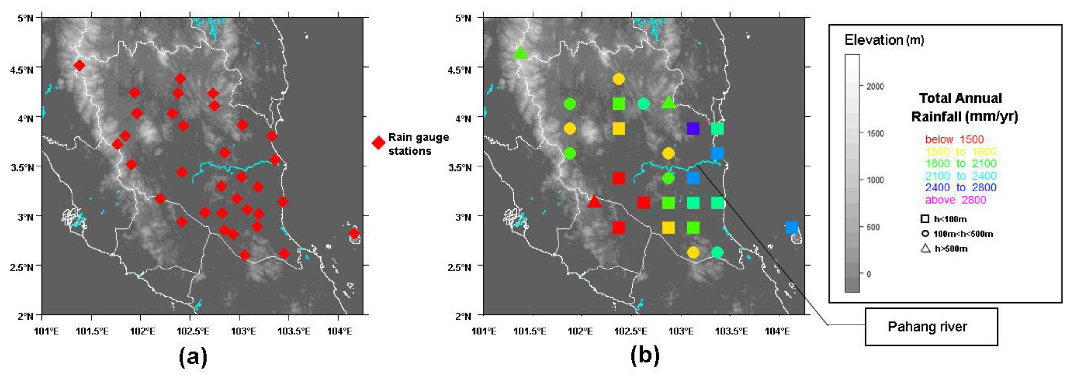
Figure 2.
The performance scores of detection metrics calculated using TRMM using the rain gauge measurement as observed. (a) POD; (b) FAR; (c) POFD; and (d) TS.
Figure 2.
The performance scores of detection metrics calculated using TRMM using the rain gauge measurement as observed. (a) POD; (b) FAR; (c) POFD; and (d) TS.

Figure 3.
The performance scores of volumetric metrics calculated using TRMM using the rain gauge measurement as observed. (a) RMSE; (b) PBIAS; (c) NSE; and (d) CC.
Figure 3.
The performance scores of volumetric metrics calculated using TRMM using the rain gauge measurement as observed. (a) RMSE; (b) PBIAS; (c) NSE; and (d) CC.

Figure 4.
Rainfall volumetric metric performance at different elevation regions. (a) POD; (b) FAR; (c) POFD; (d) TS; (e) RMSE; (f) PBIAS; (g) NSE; and (h) CC.
Figure 4.
Rainfall volumetric metric performance at different elevation regions. (a) POD; (b) FAR; (c) POFD; (d) TS; (e) RMSE; (f) PBIAS; (g) NSE; and (h) CC.

Figure 5.
TRMM performance in terms of percent bias (PBIAS) by each season.

Figure 6.
The performance scores of detection metrics after bias adjustment.
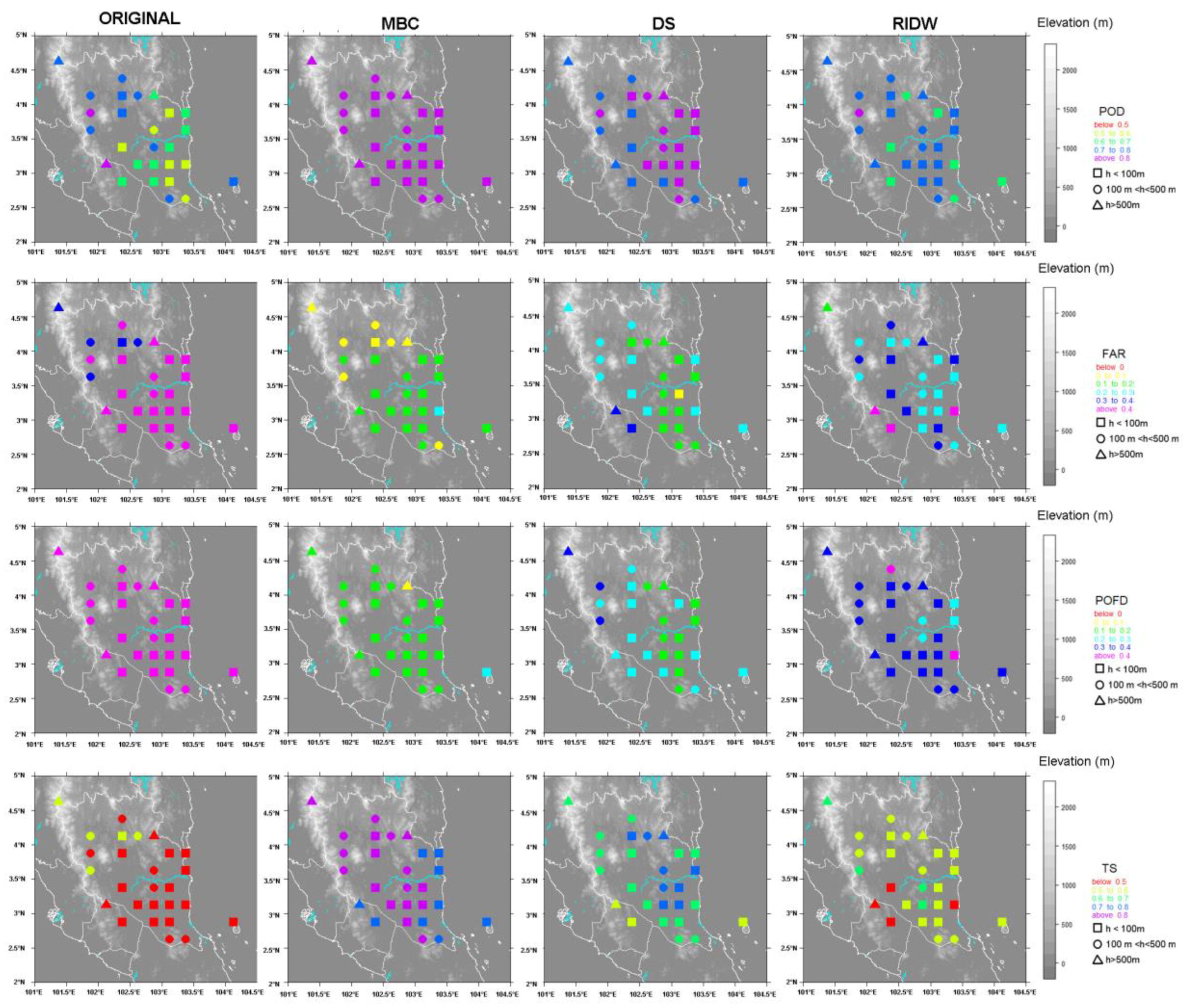
Figure 7.
The performance scores of volume metrics after being bias adjusted.
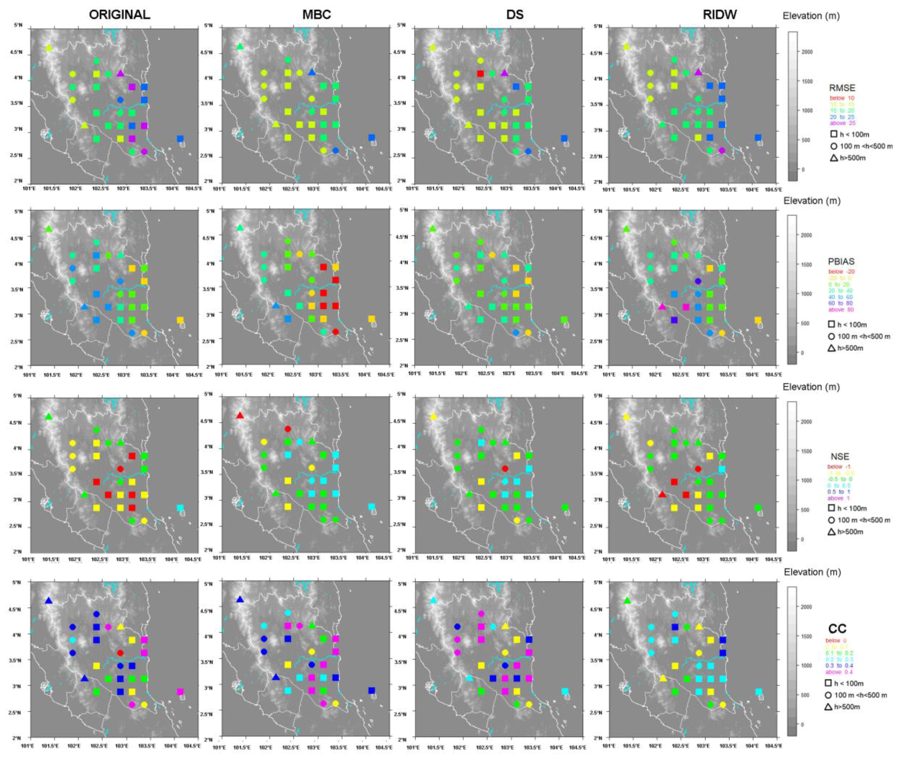
Table 1.
Number of pixel-point pairs.
| No. of Stations | No. of TRMM Pixel- Rain Gauge Point Pairs | No. of Stations Based on the Altitude | ||
|---|---|---|---|---|
| Low-Altitude (h < 100 m) | Mid-Altitude (100 m < h < 500 m) | High-Altitude (h > 500 m) | ||
| 32 | 27 | 15 | 9 | 3 |
Table 2.
Detection metrics to be used in the study (Sakolnakhon (2013)).
| No. | Detection Metrics | Explanation | Equation |
|---|---|---|---|
| 1 | The probability of detection (POD) or the hit rate |
| ** |
| 2 | The false alarm ratio (FAR) |
| ** |
| 3 | The probability of false detection (POFD) or the false alarm rate |
| ** |
| 4 | The threat score (TS) or critical success index (CSI) |
| ** |
Where a, b, c, and d are the numbers of events observed shown in Table 3.
Table 3.
Contingency table for category estimates of a point to point event, where a, b, c, and d are the numbers of events observed (Sakolnakhon (2013)).
Table 3.
Contingency table for category estimates of a point to point event, where a, b, c, and d are the numbers of events observed (Sakolnakhon (2013)).
| Estimate | Observed | Total | |
|---|---|---|---|
| Yes | No | ||
| Yes | a (HIT) | b (FALSE ALARM) | a + b |
| No | c (MISS) | d (CORRECT REJECTION) | c + d |
| Total | a + c | b + d | a + b + c + d = n |
Table 4.
Standard verification indices for evaluating the TRMM rainfall data (Sources: Tan & Duan (2017) [28]; Zambrano-Bigiarini (2014) [29]).
| No. | Methods | Explanation | Equation |
|---|---|---|---|
| 1 | Root Mean Square Error (RMSE) |
| * |
| 2 | Nash Sutcliffe Efficiency (NSE) |
| * |
| 3 | Percentage Bias (PBIAS) |
| * |
| 4 | The correlation coefficient (CC) |
| * |
Where Si is the estimated values, Oi is the observed values and N is the number of samples.
Table 5.
The detection performance scores calculated using TRMM using the rain gauge measurement.
| TRMM PIXEL ID | Station Name | Elevation (m) | COORDINATES | Average Annual Rainfall (mm) | POD | FAR | POFD | TS | |
|---|---|---|---|---|---|---|---|---|---|
| Long | Lat | ||||||||
| 450219 | Gunung Brinchang di C.Highlands | 1736 | 101.375 | 4.625 | 2091.719 | 0.775 | 0.324 | 0.520 | 0.566 |
| 451015 | Kuala Marong | 223 | 101.875 | 3.625 | 2139.778 | 0.749 | 0.366 | 0.572 | 0.523 |
| Bukit Peninjau | |||||||||
| 451016 | Stor JPS Raub | 143 | 101.875 | 3.875 | 1889.919 | 0.807 | 0.450 | 0.548 | 0.486 |
| 451017 | Bukit Betong | 151 | 101.875 | 4.125 | 2018.206 | 0.749 | 0.367 | 0.598 | 0.523 |
| JKR Benta | |||||||||
| 451413 | Simpang Pelangai | 546 | 102.125 | 3.125 | 1495.813 | 0.806 | 0.550 | 0.549 | 0.406 |
| 451812 | Ldg. Glendale | 86 | 102.375 | 2.875 | 1326.756 | 0.651 | 0.596 | 0.529 | 0.332 |
| 451814 | Jps. Temerloh | 43 | 102.375 | 3.375 | 1281.556 | 0.594 | 0.556 | 0.437 | 0.341 |
| 451816 | Rumah Pam Paya Kangsar | 61 | 102.375 | 3.875 | 1901.238 | 0.785 | 0.484 | 0.588 | 0.452 |
| 451817 | Kg. Sg. Yap | 70 | 102.375 | 4.125 | 1932.072 | 0.774 | 0.361 | 0.621 | 0.539 |
| Kg. Merting | |||||||||
| 451818 | Kuala Tahan | 103 | 102.375 | 4.375 | 1848.825 | 0.797 | 0.443 | 0.547 | 0.488 |
| 452213 | Pos Iskandar | 53 | 102.625 | 3.125 | 1410.544 | 0.653 | 0.550 | 0.502 | 0.363 |
| 452217 | Ulu Tekai (A) | 292 | 102.625 | 4.125 | 2524.606 | 0.768 | 0.397 | 0.562 | 0.510 |
| 452612 | Ulu Sg.Chanis | 76 | 102.875 | 2.875 | 1708.791 | 0.671 | 0.452 | 0.644 | 0.432 |
| 452613 | Sg. Kepasing | 78 | 102.875 | 3.125 | 2041.4 | 0.676 | 0.412 | 0.640 | 0.459 |
| Bkt. Ibam | |||||||||
| 452614 | Sg. Cabang Kanan | 157 | 102.875 | 3.375 | 2038.463 | 0.741 | 0.513 | 0.625 | 0.416 |
| 452615 | Pintu Kawalan Paya Kertam | 110 | 102.875 | 3.625 | 1676.019 | 0.572 | 0.533 | 0.477 | 0.346 |
| 452617 | Kawasan ‘B’ Ulu Tekai | 565 | 102.875 | 4.125 | 2178.175 | 0.635 | 0.439 | 0.421 | 0.424 |
| 453011 | Kg. Kedaik | 132 | 103.125 | 2.625 | 1710.381 | 0.774 | 0.504 | 0.552 | 0.433 |
| 453012 | Pecah Batu Bkt. Raidan | 46 | 103.125 | 2.875 | 2209.75 | 0.556 | 0.521 | 0.472 | 0.347 |
| 453013 | Temeris | 40 | 103.125 | 3.125 | 2303.394 | 0.560 | 0.430 | 0.560 | 0.393 |
| 453014 | Kg. Unchang | 27 | 103.125 | 3.375 | 2578.45 | 0.623 | 0.418 | 0.701 | 0.430 |
| Kg. Batu Gong | |||||||||
| 453016 | Sg. Lembing P.C.C.L Mill | 29 | 103.125 | 3.875 | 3073.263 | 0.540 | 0.449 | 0.494 | 0.375 |
| 453411 | Sg. Anak Endau Kg. Mok | 162 | 103.375 | 2.625 | 2463.394 | 0.587 | 0.472 | 0.465 | 0.385 |
| 453413 | Dispensari Nenasi di Pekan | 11 | 103.375 | 3.125 | 2301.631 | 0.551 | 0.622 | 0.610 | 0.289 |
| 453415 | Rumah Pam Pahang Tua di Pekan | 18 | 103.375 | 3.625 | 2762.063 | 0.632 | 0.562 | 0.684 | 0.349 |
| 453416 | Pejabat JPS Negeri Pahang | 0 | 103.375 | 3.875 | 2511.481 | 0.621 | 0.579 | 0.668 | 0.335 |
| 454612 | Takek, Pulau Tioman | 0 | 104.125 | 2.875 | 2619.363 | 0.761 | 0.432 | 0.486 | 0.482 |
Table 6.
The volumetric performance scores calculated using TRMM using the rain gauge measurement.
| TRMM PIXEL ID | Station Name | Elevation (m) | COORDINATES | Average Annual Rainfall (mm) | RMSE (mm/day) | PBIAS (%) | NSE | CC | |
|---|---|---|---|---|---|---|---|---|---|
| Long | Lat | ||||||||
| 450219 | Gunung Brinchang di C.Highlands | 1736 | 101.375 | 4.625 | 2091.719 | 12.801 | 9.4 | −0.238 | 0.379 |
| 451015 | Kuala Marong | 223 | 101.875 | 3.625 | 2139.778 | 14.702 | 32.5 | −0.53 | 0.316 |
| Bukit Peninjau | |||||||||
| 451016 | Stor JPS Raub | 143 | 101.875 | 3.875 | 1889.919 | 15.292 | 50.8 | −0.747 | 0.281 |
| 451017 | Bukit Betong | 151 | 101.875 | 4.125 | 2018.206 | 14.74 | 36.6 | −0.59 | 0.309 |
| JKR Benta | |||||||||
| 451413 | Simpang Pelangai | 546 | 102.125 | 3.125 | 1495.813 | 13.205 | 53.9 | −0.477 | 0.351 |
| 451812 | Ldg. Glendale | 86 | 102.375 | 2.875 | 1326.756 | 15.055 | 54.9 | −0.855 | 0.168 |
| 451814 | Jps. Temerloh | 43 | 102.375 | 3.375 | 1281.556 | 16.836 | 50.6 | −1.124 | 0.033 |
| 451816 | Rumah Pam Paya Kangsar | 61 | 102.375 | 3.875 | 1901.238 | 15.259 | 34.7 | −0.538 | 0.318 |
| 451817 | Kg. Sg. Yap | 70 | 102.375 | 4.125 | 1932.072 | 14.526 | 45.2 | −0.966 | 0.377 |
| Kg. Merting | |||||||||
| 451818 | Kuala Tahan | 103 | 102.375 | 4.375 | 1848.825 | 17.194 | 35.6 | −0.495 | 0.343 |
| 452213 | Pos Iskandar | 53 | 102.625 | 3.125 | 1410.544 | 16.345 | 46.9 | −1.176 | 0.145 |
| 452217 | Ulu Tekai (A) | 292 | 102.625 | 4.125 | 2524.606 | 16.068 | 14.1 | −0.078 | 0.498 |
| 452612 | Ulu Sg.Chanis | 76 | 102.875 | 2.875 | 1708.791 | 14.185 | 37.4 | −0.852 | 0.392 |
| 452613 | Sg. Kepasing | 78 | 102.875 | 3.125 | 2041.4 | 15.974 | 26 | −0.99 | 0.316 |
| Bkt. Ibam | |||||||||
| 452614 | Sg. Cabang Kanan | 157 | 102.875 | 3.375 | 2038.463 | 18.766 | 18.6 | −0.193 | 0.347 |
| 452615 | Pintu Kawalan Paya Kertam | 110 | 102.875 | 3.625 | 1676.019 | 21.307 | 48.6 | −2.149 | -0.004 |
| 452617 | Kawasan ‘B’ Ulu Tekai | 565 | 102.875 | 4.125 | 2178.175 | 29.87 | 30.3 | −0.469 | 0.028 |
| 453011 | Kg. Kedaik | 132 | 103.125 | 2.625 | 1710.381 | 16.486 | 46.2 | −0.282 | 0.459 |
| 453012 | Pecah Batu Bkt. Raidan | 46 | 103.125 | 2.875 | 2209.75 | 25.269 | 18.9 | −1.102 | 0.01 |
| 453013 | Temeris | 40 | 103.125 | 3.125 | 2303.394 | 23.259 | 19.5 | −1.261 | 0.105 |
| 453014 | Kg. Unchang | 27 | 103.125 | 3.375 | 2578.45 | 19.957 | 9.3 | −0.648 | 0.394 |
| Kg. Batu Gong | |||||||||
| 453016 | Sg. Lembing P.C.C.L Mill | 29 | 103.125 | 3.875 | 3073.263 | 27.116 | −4.2 | −1.257 | 0.043 |
| 453411 | Sg. Anak Endau Kg. Mok | 162 | 103.375 | 2.625 | 2463.394 | 28.563 | −4.5 | −0.614 | 0.035 |
| 453413 | Dispensari Nenasi di Pekan | 11 | 103.375 | 3.125 | 2301.631 | 26.936 | 14 | −0.775 | 0.167 |
| 453415 | Rumah Pam Pahang Tua di Pekan | 18 | 103.375 | 3.625 | 2762.063 | 22.502 | −2 | −0.007 | 0.46 |
| 453416 | Pejabat JPS Negeri Pahang | 0 | 103.375 | 3.875 | 2511.481 | 22.924 | 14.8 | −0.366 | 0.405 |
| 454612 | Takek, Pulau Tioman | 0 | 104.125 | 2.875 | 2619.363 | 21.654 | −10.4 | 0.093 | 0.44 |
Table 7.
Average performance scores of pre-corrected TRMM and post-corrected TRMM (MBC, DS, RIDW).
| Pre-Corrected Scores (Original) | Post-Corrected Scores | |||
|---|---|---|---|---|
| MBC | DS | RIDW | ||
| POD | 0.682 | 0.911 | 0.804 | 0.722 |
| FAR | 0.473 | 0.126 | 0.213 | 0.298 |
| POFD | 0.558 | 0.142 | 0.238 | 0.336 |
| TS | 0.423 | 0.806 | 0.662 | 0.552 |
Table 8.
Average performance scores of pre-corrected TRMM and post-corrected TRMM (MBC, DS, RIDW).
| Pre-Corrected Scores (Original) | Post-Corrected Scores | |||
|---|---|---|---|---|
| MBC | DS | RIDW | ||
| RMSE (mm/day) | 19.140 | 15.621 | 15.863 | 17.944 |
| PBIAS (%) | 26.952 | 3.904 | 13.544 | 30.233 |
| NSE | −0.692 | −0.260 | −0.264 | −0.524 |
| CC | 0.264 | 0.307 | 0.289 | 0.186 |
© 2018 by the authors. Licensee MDPI, Basel, Switzerland. This article is an open access article distributed under the terms and conditions of the Creative Commons Attribution (CC BY) license (http://creativecommons.org/licenses/by/4.0/).
Share and Cite
MDPI and ACS Style
Mohd Zad, S.N.; Zulkafli, Z.; Muharram, F.M. Satellite Rainfall (TRMM 3B42-V7) Performance Assessment and Adjustment over Pahang River Basin, Malaysia. Remote Sens. 2018, 10, 388. https://doi.org/10.3390/rs10030388
AMA Style
Mohd Zad SN, Zulkafli Z, Muharram FM. Satellite Rainfall (TRMM 3B42-V7) Performance Assessment and Adjustment over Pahang River Basin, Malaysia. Remote Sensing. 2018; 10(3):388. https://doi.org/10.3390/rs10030388
Chicago/Turabian StyleMohd Zad, Siti Najja, Zed Zulkafli, and Farrah Melissa Muharram. 2018. "Satellite Rainfall (TRMM 3B42-V7) Performance Assessment and Adjustment over Pahang River Basin, Malaysia" Remote Sensing 10, no. 3: 388. https://doi.org/10.3390/rs10030388
Note that from the first issue of 2016, this journal uses article numbers instead of page numbers. See further details here.