Sparse Subspace Clustering-Based Feature Extraction for PolSAR Imagery Classification


1
Key Laboratory of Intelligent Perception and Image Understanding of Ministry of Education, Xidian University, Xi’an 710071, China
2
Joint International Research Laboratory of Intelligent Perception and Computation, Xidian University, Xi’an 710071, China
*
Author to whom correspondence should be addressed.
Remote Sens. 2018, 10(3), 391; https://doi.org/10.3390/rs10030391
Submission received: 8 January 2018
/
Revised: 21 February 2018
/
Accepted: 27 February 2018
/
Published: 2 March 2018
(This article belongs to the Special Issue Classification and Feature Extraction for Remote Sensing Image Analysis)
Abstract
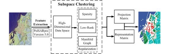
:Features play an important role in the learning technologies and pattern recognition methods for polarimetric synthetic aperture (PolSAR) image interpretation. In this paper, based on the subspace clustering algorithms, we combine sparse representation, low-rank representation, and manifold graphs to investigate the intrinsic property of PolSAR data. In this algorithm framework, the features are projected through the projection matrix with the sparse or/and the low rank characteristic in the low dimensional space. Meanwhile, different kinds of manifold graphs explore the geometry structure of PolSAR data to make the projected feature more discriminative. Those learned matrices, that are constrained by the sparsity and low rank terms can search for a few points from the samples and capture the global structure. The proposed algorithms aim at constructing a projection matrix from the subspace clustering algorithms to achieve the features benefiting for the subsequent PolSAR image classification. Experiments test the different combinations of those constraints. It demonstrates that the proposed algorithms outperform other state-of-art linear and nonlinear approaches with better quantization and visualization performance in PolSAR data from spaceborne and airborne platforms.

1. Introduction
Polarimetric synthetic aperture image (PolSAR) is an actively full polarimetric radar measurement system, which can acquire abundant electromagnetic scattering information according to different transmitting and receiving mechanisms. Due to the comprehensive description of land covers, the received data contains more target information to deal with target detection, recognition, and land cover classification tasks. Recently, a large amount of data from airborne and spaceborne platforms has been produced. However, the development of assistant analysis and automatic decision systems have lagged far behind the production of data sources. The distinctive imaging mechanism and the complexity of imaging conditions make it difficult to automatic interpret and manual adjudge PolSAR data. Then, how to process, analyze, and exploit the large amount of PolSAR data, and how to extract more effective target information have become an key research direction in the field of remote sensing information processing.
In the field of radar polarimetry signal processing, the observation data including polarimetry covariance matrix, coherent matrix, backscattering matrix, Stokes matrix, and Mueller matrix can be calculated through mathematical operation to characterize the polarimetric scattering property. Meanwhile, in order to exploit the distinct physical mechanism, some polarimetric target decomposition mechanisms have been developed to describe the average backscattering of some independent components. In an early example of this, Krogagor carried out a study and resolved the scattering matrix into three components with clear physical mechanism [1]. Cloude [2], Holm and Barnes, and Van Zyl [3] also developed excellent orthogonal component decomposition theorems. Freeman developed a three-components mechanism to capture canopy scatter from a cloud of randomly oriented dipoles, which is usable to estimate the effects of foresee inundations [4]. Furthermore, the helix scattering term taking account of the co-pol and the cross-pol correlations is added as the fourth component in the three components scattering model [5]. Based on H/A/ (Cloude) decomposition, it can initialize and develop the Wishart-distribution based maximum likelihood classifier [6,7]. Those polarimetric characteristics were attempted to improve the classification performance and exploited to discriminate different targets. However, how to select and extract effective features from PolSAR data is still a problem in the PolSAR image processing. This is because the different target decomposition components represent different physical mechanisms, and the same targets or terrains always possess the same scattering mechanism, and vice versa [8]. Some approaches directly extract nine freedom parameters from coherence matrix or covariance matrix to construct a feature vector in machine learning related algorithms. They are also regarded as the representative features for multilook PolSAR image interpretation [9]. The covariance matrix is the Hermitian positive definite matrix lying in the nonlinear manifolds, so some researchers hold that Riemannian geometry is suitable to analyze the PolSAR data, and project the matrix into a higher dimensional kernel Hilbert space [10]. Literatures [11,12] evaluate and compare features for classifying PolSAR imagery, and some also cascade multimodal features to form high-dimensional vectors and reduce those vectors to discriminative features [8,13,14] .
Considering the spatial correlation of pixels in imagery, literature [15] focuses on combining of multimodal features and exploiting the tensor-based techniques to facilitate the PolSAR image classification. Some literatures [16,17] exploit the segmentation steps or the superpixel algorithms to form groups of pixels to represent homogenous regions. Their features can reduce the influence of speckles and the computation complexity. However, there are some problems in the process of features selection and extraction. Different classifiers are suitable for different features owing to different physical and statistical characteristics. So it is difficult to select optimal features in corresponding classification tasks to adapt to different land covers. Then, the conventional methods cascade multimodal features into a high-dimensional space, and project the data into a low-dimensional space. In other words, they are dimensionality reduction process. In the principal component analysis (PCA) and independent component analysis (ICA) algorithms [18,19,20], they mainly focus on investigating the discriminative components of a group of data. In order to test whether it is suitable to construct a whole neighborhood graph, Laplacian eigenmaps (LE) tried to process the features from PolSAR data [8,21]. Graph embedding methods utilize the training samples to calculate the similarity matrix with a linear technology and project the data into a low-dimensional space [13]. However, those embedding or clustering algorithms are all based on eigenvalue decomposition without straightforward extension for out-of-sample examples. To overcome those difficulties, we devote our work to sufficiently exploiting a latent intrinsic subspace and calculating a corresponding projection matrix for extracting the discriminative features.
In the pattern recognition field, no matter whether the process is text, video, document, audio, or images, high-dimensional data problem is inevitable. However, those high-dimensional data often lie in a union of low-dimensional subspace. It is necessary to recover the low-dimensional structures for reducing the computation complexity and improving the performance of algorithm tasks [22]. In many problems, data from the same category can be represented by a union of low-dimensional space. Then the notion of subspace clustering is proposed to focus on finding the number of subspaces, the intrinsic dimension of corresponding subspace, and the basic of subspaces [23]. The subspace clustering algorithms can be mainly divided into four categories: iterative methods, algebraic approaches, statistical methods, and spectral clustering based methods [24,25,26,27,28,29]. Meanwhile, the sparse representation and low-rank based algorithms are proposed to process the subspace cluster problem archiving great success. Those state-of-the-art algorithms include the Sparse Subspace Clustering (SSC) [22,30,31], Low-Rank Subspace Clustering (LRSC) [32,33], Low-Rank Sparse Subspace Clustering (LRSSC) [34], and Laplacian regularized Low Rank Subspace Clustering (LapLRSC) [35] under the constraint of sparsity, low-rank and manifold regularization to find a reasonable representation of data. They could handle the noises and outliers in the dataset without knowing the number of dimension of subspaces. Motivated by those works, we make use of the property of subspace cluster algorithms to explore the intrinsic subspace of the combination high-dimensional feature vectors, and calculate corresponding projection matrix for extracting intrinsic features form the PolSAR data.
In this paper, we propose the novel subspace cluster based methods to process the PolSAR imagery classification. It analyzes the extracted features and classification effect under different constraints, and investigates the algorithm performance in the reproducing kernel Hilbert space. It gives the contribution as follows. First, the related comprehensive feature vectors are extracted from PolSAR data, which come from many target decomposition algorithms including the power of components in coherent (Krogager) [1] and incoherent decompositions (Freeman, Yamaguchi, Van Zyl, Neumann) [4,5,36], and the parameters with definitely physical characteristics from H/A/ [37,38] and Touzi decompositions [39]. Most of them can be easily realized by PolSARpro5.0 software (http://earth.esa.int/polsarpro) [40]. Second, the projection matrix and affinity matrix can be calculated simultaneously under the constraints of sparse representation (SR) [22,41], low rank representation (LLR) [33], and manifold regularizations (MR), or various combinations of those terms [42]. In those terms, the SR acts to select a few points from the same subspace, the LLR captures the global structure of samples, and the MR detects the local manifold structure of data.The algorithm aims at finding groups of data points from different subspace in samples space. Meanwhile, we test the data in high-dimensional Hilbert space. Third, because of the deficiency of training samples in remote sensing data, the unsupervised method is proposed with straightforward extension ability. The projection matrix is optimized directly from the learning algorithm which solves the out-of-sample problem without recomputing eigenvectors.
This paper is organized as follows. In Section 2, We introduce background of the subspace cluster problem and review the related works about SSC, LRSC, and LRSSC. Section 3 introduces the proposed manifold regularized sparse and the latent subspace clustering methods for the PolSAR data. Section 4 presents the experiment results of proposed method and contrast methods, and gives the experiment analysis. Finally, discussion and some conclusions are drawn in Section 5 and Section 6 respectively.
2. Related Work of Proposed Method
In order to search for a few points from the PolSAR samples and capture the global structure of PolSAR data, it is necessary to introduce the background of proposed method, i.e., subspace clustering problem. Subspace clustering is an extension of the traditional clustering method, which localizes the relevant dimensions and looks for the groups of similar samples for clustering. It can be utilized in removing irrelevant and redundant dimensions though analysing the entire dataset. Based on those algorithms, we could evaluate the intrinsic subspaces of the dataset and weed out the redundant information in the multimodal PolSAR features.
The following sentences summarize the subspace clustering problem and briefly introduce the low-rank and sparse subsapce clustering algorithms. Let be a collection of N data points drawn from a group of K independent linear subspace with the dimensionality and the bases . Let be the given union of data points from the subspace i. The target of this problem is to find the number of subspace K, the basis of each subspace, the corresponding dimensions, and the segmentation of the data from a collection of multisubspace data. The specified segmentation data matrix is , in which and denotes the total number of data points and a unknown permutation matrix. Those subspace basis can be chosen from the columns of the data matrix . Some related methods can be employed to find the basis to cluster the signals according to their subspace.
2.1. Sparse Subspace Clustering
As above, the solution can be restricted by the norm to sparsely represent the point in dictionary . Then it can be formulated as:
in which, denotes the representation coefficient of . The constraint eliminates the linear combination to represent the point itself, the sparsity means the nonzero elements in coefficient equal or less than . The dictionary is a self-representation matrix, the points in it can be reconstructed by a combination of other points. To obtain the solution of norm, it needs to be relaxed as a non-convex problem to find the sparse representation of . Then a -norm () is employed to replace norm to minimize the formulation,
which can be solved by some convex relaxation optimization tools. For efficient computing, it covers all data points in matrix form and can be transformed as
in which is the representation coefficient matrix whose i-th column denotes the representation vector of in dictionary . The vector refers to the diagonal elements of equaling to 0, which means data point can’t be self-represented by itself. However, in real applications, some noise, outliers and errors exist in data corrupting process or measurement in the data collection techniques. Then the real data may lie in a union of affine subspace that is regarded as a more general model rather than linear subspace. To deal with this problem, we always consider the fact that in an affine subspace with the dimensionality can be linearly represented by other sample points in subspace [20].
This formulation includes the linear equality constraints, denotes the sum of entries in each representation vector equaling to 1, and means to minimize the power of noise.
2.2. Low-Rank Representation Subspace Clustering
LRR subspace cluster is an important clustering algorithm. It aims at finding the lowest-rank representation of a collection of vectors jointly, which can be better capture the global structure of data [33]. Low rank may be a more appropriate and robust technique to capture the global structure of data. It demands to find a “lowest-rank representation” of data with respect to the dictionary
The above formulization is nonconvex due to the discrete nature property of rank function. Then a convex transformation is provided as follows:
in which is the nuclear norm, i.e., the sum of singular value of the matrix [43]. In order to segment the data into the corresponding subspace, we compute an affinity matrix to encode the pairwise affinities matrix data vectors. Then the sample matrix is utilized as a dictionary to exploit the intrinsic data similarity,
Because of the solution space is , it has the advantage over the spare representation method that there always exists a nontrivial solution without eliminating the sample point itself when optimizing. LLR also confronts the real problem that the observations are corrupted or noisy and sometimes even missing.
2.3. Low-Rank Sparse Subspace Clustering
Considering the sparse and low-rank property coexist in the data space, the authors also study for searching for a representation coefficient matrix with both the sparsity and low-rank property [23]. In the low-rank sparse clustering (LRSSC) algorithm, the sparse and low-rank norms are added into the model and the objective function is as follows:
where the parameters and balance the weighted of the sparse and low-rank norms. The optimization framwork can be solved by the alternative direction method of multipliers (ADMM) [44]. Similar to SSC and LRSSC algorithms, after obtained the representation matrix , we can define the weighted matrix as follows:
3. Latent Subspace Clustering for PolSAR Classification
Considering the lack of the manually labeled samples in PolSAR data, it is necessary to accurately approximate data structure and analyze the intrinsic data dimensionality for subsequent classification and segmentation. For modeling and evaluating the multimodal high-dimensional features, the structure should be considered both in terms of local and global information properties. The global information can be captured by the sparse representation and low-rank approximation model. These algorithms aim at finding a representation matrix of data samples to construct the similarity matrix. However, under the common assumption of the spectral clustering-based method: the nearest neighbors of a sample are in the same subspace of this sample. According to the local similarity to classify the samples in a same category. Both the local and global thoughts have disadvantages. The global representation techniques are sensitive to outliers and noise, while the local spectral algorithms ignore the samples that may be in the same subspace far away form each other.
To resolve these drawbacks and consider the practical applications, a manifold graph is added to the representation framework to capture the local geometry of data, while the LRR or the sparsity enhance the data global description in subspace clustering [45,46]. The manifold graph can actually approximate the nonlinear structures existing in the PolSAR data, which can effective preserve the local geometric structure embedded in the high-dimensional PolSAR data space. Then we resort to making use of the local geometry information in learning techniques for calculating the similarity of each point. How to construct an undirected nearest graph is the basic step to characterize the local structure of PolSAR data. We analyze some manifold graphs from different perspectives to consider the relationship and measure the similarity of PolSAR data points. This is due to the high complexity of eigenvalue decomposition from the spectral based methods. The PolSAR images are preprocessed by the superpixel algorithms to reduce the algorithm complexity in optimization. We select a normalized cut technique based on superpixel algorithms to oversegment PolSAR images and regard one superpixel as a resolution unit in the spectral clustering methods [47].
In PolSAR image classification, it is necessary to search for a suitable graph to characterize the polarimetric property for obtaining better classification performance. In general, the most common ways to define neighborhood graph are k-nearest neighbor mode and -neighbor mode. In this section we will analyze the graph constructed in the k-nearest neighbor mode, and three kinds of methods are employed to form manifold regularization to capture the geometry structure in PolSAR data.
3.1. Manifold Graph Construction for PolSAR Data
The graph idea employed in the subspace clustering is inspired by the spectral clustering algorithms [48]. Given a group of data points , it is necessary to compute the weighted and undirected graph , in which V denotes the vertex set and E denotes the edge set associated with weights . We can build the nearest graph G with the points corresponding to vertexes and the similarity of points corresponding to the weight matrix , respectively. When we have achieved the matrix , we can obtain the degree matrix that is a diagonal matrix measuring the similarity between point i and other points. Then a normalized graph Laplacian matrix can be computed.
a. The similarity is directly measured by the Euclidean distance of the concatenation feature vectors from the PolSAR data, and the matrix of graph can be defined as follows:
b. In order to capture the complex statistical information in PolSAR data, some measures are derived from the complex Wishart distribution in the coherency matrix [49]. Under the three general metric apply conditions: generalized non-negativity, identity of discernible, symmetry and subadditivity, the Bartlett distance and symmetry revised Wishart distance (SRW) are proposed to measure the pairwise similarities between different PolSAR pixels [16]. The SRW distance will be utilized to construct the weighted matrix:
where and is the coherence matrix representing the pixel and , and the K-nearest neighbors are also measured by SRW distance. The parameter is the Gaussian kernel bandwidth.
c. The features are extracted by different methods and may be in different modalities. In order to effectively combine multiple graph layers by laying multiple feature spaces, a Grassmann manifold provided a nature framework to solve this problem [50]. Given a set of points, this can be represented by the feature vectors from Z feature spaces. We first compute the feature space representation matrix by the spectral clustering algorithm, which can be solved through the trace minimization problem:
in which n denotes the number of vertices in the z-th graph, and k denotes the target number of clusters. The graph Laplacian matrix is first computed corresponding to each graph which is represented by the spectral embedding matrix . The column in matrix is the eigenvector corresponding to the i-th largest eigenvalue of the matrix . The philosophy of merging multi-layer graphs is to find a representative space closed to all the individual space and the representation matrix preserving the vertexes connection information in each graph. The merging Laplacian matrix is calculated to represent the multi-layer graphs through mathematical derivation and the Rayleigh-theorem solution [50,51].
where regularization parameter balances the effluence between Graph Laplacian and the spectral embedding matrix .
3.2. Manifold Graph Regularized Low-Rank Subspace Clustering
The similarity measurement and the weighted matrix calculation are the foundations to construct the undirected nearest neighbor graph. A suitable manifold graph construction determines the algorithms to explore the data intrinsic data structure. The manifold information is maintained by the graph regularization in the liner models to model the nonlinear properties of PolSAR data. The local geometric structures of high-dimensional data are also preserved by the Laplacian graph. The manifold graph can be directly utilized in manifold based dimensionality reduction techniques and spectral clustering methods, or computed as a regularized trace term added into the sparsity and LRR framework. Matrix is always regarded as a prior to achieve the uncontaminated data samples [35,52]. Under the assumption that if tow data points i and j are closed in the geometry space, then the representation of two points are also closed to each other [46,53,54]. The regularization can be added to constrain the representation matrix subjecting to the data geometry structure [42,55].
The above related manifold regularizations are incorporated by the term in LRR algorithm, then the Laplacian regularized LRR (LapLRR) model is formulated as follows [42]:
In this model, the global data structure are captured by the nuclear norm . According to different Laplacian regularization construction models, we can combine Equation (14) with three Laplacian regularized models to form three subspace clustering algorithms including Euclidean distance based LapLRSC (LapLRSC-ED), SRW distance based LapLRSC (LapLRSC-SRW), and multi graph model based LapLRSC (LapLRSC-MulG) algorithms.
3.3. Laplacian Manifold Regularized Latent Subspace Clustering
For PolSAR Classification, it also required to investigate the latent subspace distribution in feature space. However, how to process cascaded high dimensional feature vector is also a problem. In this paper, we simultaneously introduce the Laplacian manifold regularization and LRR constraint to capture the data structure and analyze the sparsity of observation samples. Because of the complexity of the PolSAR data, we analyze the feature with some typical subspace clustering algorithms to embed the high-dimensional feature into an intrinsic low-dimensional feature space. Then a Laplacian manifold regularized low-rank sparse subspace (LapLSSC) algorithm formulated as follows aims to explore the low-dimensional latent subspace :
For the large-scale PolSAR classification problem, the projection matrix is exploited to solve the out-of-sample problems. A PCA-like regularization term is added to ensure the projection domain keeping enough information from the original domain. Then the projection matrix and the comprehensive representation matrix can simultaneously computed from the following objective function:
where makes sure that the projection matrix is orthogonal, and it should be normalized to unit norm. Then we can divide this objective function into two parts:
in which,
is a information preservation term to obtain projection matrix. This is similar to the reconstruction error used in LRR, LRSC, SSC, and LapLRSSC algorithms. is a non-regularization parameter that balance the influence of two error terms. is a constraint term constructing by sparse, low-rank, manifold or association of those representation terms. When , the sparse representation is sought and similar to SSC. When , it pursues to a global low-rank representation. It also can be combined with different manifold regularization terms or associated with each other to form similar to LRSSC, or pursuing to manifold regularized low rank representation. In this paper, we also exploit both sparse and low-rank representation with manifold regularization that is done in LapLSSC . Parameter balance the weight of each term to influence the calculation of and .
This formulation is optimized by introducing the auxiliary variables through alternative optimization methods. The optimization process can be divided into two parts: fixed to update , and fixed to update . In order to make this objective function easier to extend to a kernel method, we replace the projection matrix as that t denotes the dimensionality of the low-dimensional embedding space. The formulation can be re-written as follows:
where is similar to a semi-definite kernel Gram matrix, and the constraint can be rewritten as . The objective function will be solved by alternative iteration method, and the overall optimization procedure is shown in Algorithm 1.
(1) Fix to update . Then we only need to select the term including variable to construct a new objective function and solve this sub-optimization problem.
Then this formula is derived through mathematical deduction and solved by the optimization approach in the literature [23,56]. The optimal solution of this objective function is:
| Algorithm 1 Solving Objective Function by Alternative Iteration Method. |
|
and are computed from the eigenvalue decomposition , and is optimized from the following formula. It is a version of the Rayleigh-Ritz theorem.
in which is derived from the following mathematical expression.
(2) Fix to update . Then we should solve the following problem with respect to the variable .
It can be optimized by ADMM method with introducing some auxiliary variables to alternatively optimize this objective function:
Then an augmented Lagrangian function is formed to solve this problem. We can minimize the following equation to obtain the optimum solution.
in which , denotes the multipliers of the constraints, and denotes the penalty parameters. This problem can be divided into five sub-problems. and are the indicator functions meaning to keep the coefficient matrix non-negative and diagonal elements of the matrix zero. and denote the updateable variables. What we need is to update one variables with fixing others to minimize those variables, each of the optimization step is summarized in Algorithm 2.
| Algorithm 2 Optimization Procedure of Equation (26). |
|
4. Experiment and Analysis
In this section, three kinds of PolSAR datasets are utilized to verify the performance of the proposed method. Before processing those datasets, a refined Lee filter [57,58] is employed to reduce the influence of speckle noise form speckle and the complicated imaging mechanism. The multimodal features are extracted from multiple polarimetric target decomposition, which is similar to literature [16] selecting features form software PolSARpro version 5.0 [40]. Those features mainly contain specific parameters and decomposition component coefficients from Van Zyl, Krogager, Yamaguchi, Neumann, TSVM, and H/A/ decompositions. They construct a 80D feature vector to represent a pixel unit.
Three state-of-the-art typical contrast approaches including liner PCA, non-linear Kernel PCA, and LE algorithms obtain low dimensional features for achieving fair comparisons. In contrast experiments, Gaussian kernel is utilized in KPCA, and the size of neighbor in LE is 12. Additional, aiming to test the influence of different constraints, we assemble sparsity and manifold constraints in with a different model to obtain the projection matrix from the constraint from SSC, LRSC, LRSSC, and LapLSSC. Those projection features computed by dimension reduction methods are employed in PolSAR image land cover classification.
We utilize Euclidean and SRW distance exploiting the graph model to compute the data neighborhood structure. The features are divided into three parts based on different target decompositions properties. The coefficients of Freeman, Krogager, Yamaguchi, Neumann, and VanZyl are taken as one modality feature, H/A/ and TSVM parameters are the other two kinds of modalities. Then a 3-layers graph regularization is constructed in Grassmann manifold. We use those manifold regularized low rank representation algorithms, LapLRSC-ED, LapLRSC-SRW, and LapLRSC-MulG to test the influence of manifold term in subspace clustering method. For LapLSSC, we choose Euclidean distance to construct the manifold describing data geometry structure.
Three assessment indicators are utilized to evaluate the performance of those techniques, including average accuracy (AA), overall accuracy (OA), and Kappa coefficient. The NN classifier is utilized to verify the effectiveness of projecting PolSAR data in low-dimensional space. The maximum iteration value of the algorithms is 10.
4.1. Introduction of PolSAR Datasets
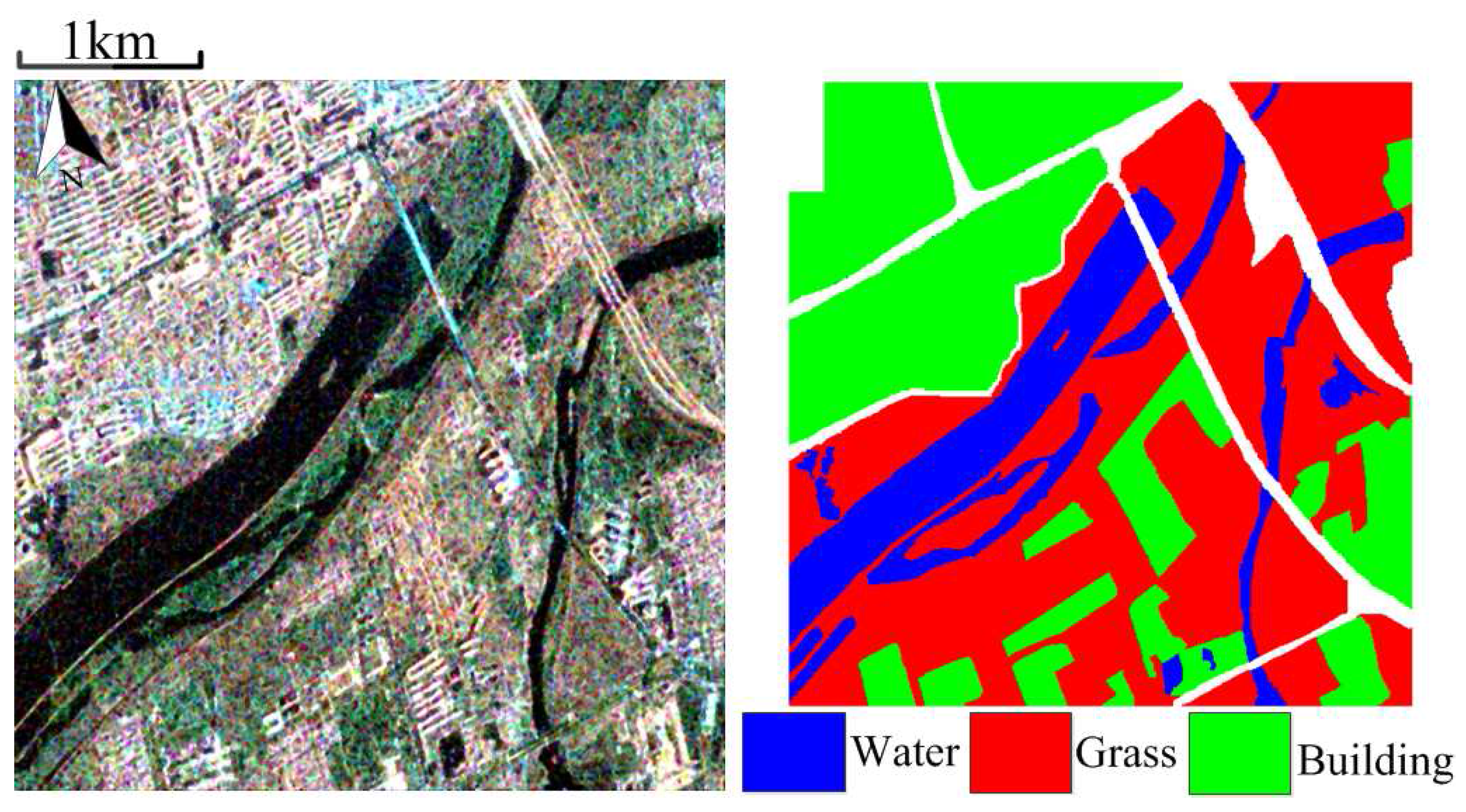
- Dataset 1: This dataset is produced in January 2010 at Fine Quad Polarization model from RADARSAT-2 sensor. This image mainly scans the region covering western Xi’an and Weihe River in Xianyang, Shaanxi Province, China. We choose one subimage with size of points and m resolution. It contains three typical terrains: buildings, grass, and water. Figure 1 shows the Pauli colored image and ground truth. The subspace clustering algorithms are carried out in this image with regularization parameters .
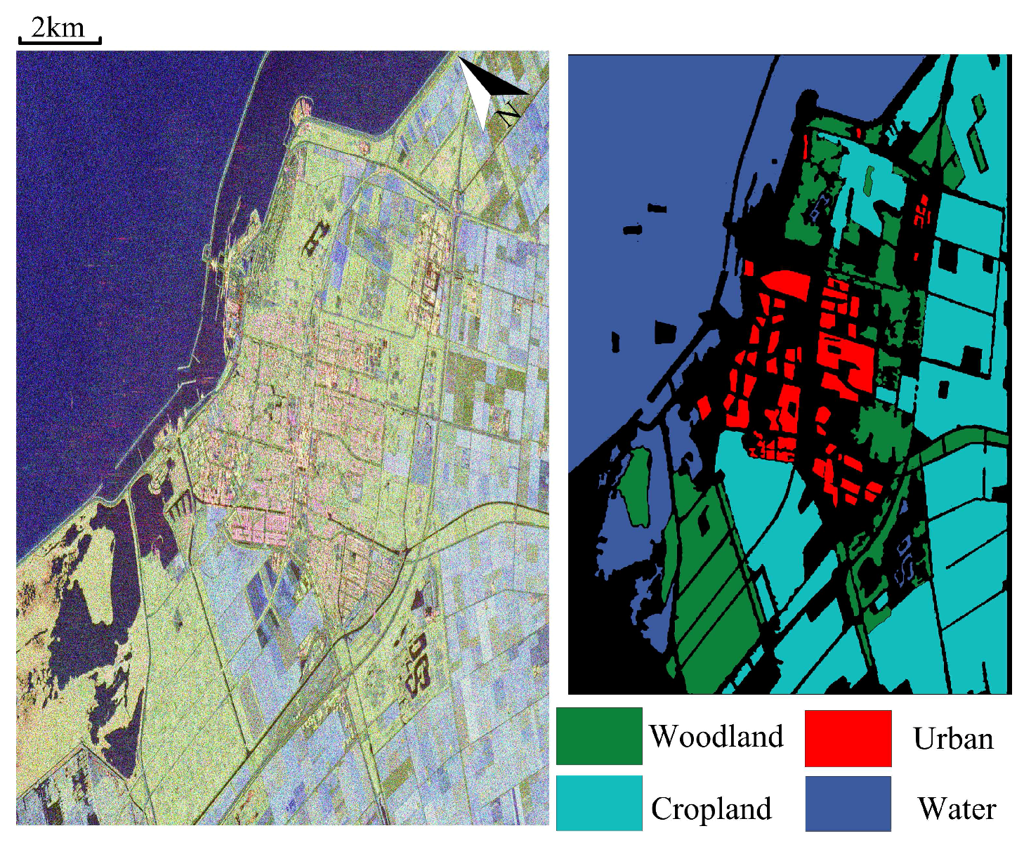
- Dataset 2: This dataset is C-band fully polarimetric data with one quad-pol mode in the RADARSAT-2 aribrone platform. This radar image scans region mainly covers Flevoland, Netherland with the size and resolution m and produced in April 2008, which is shown in Figure 2. It mainly contains four typical land covers including: woodland, cropland, urban area, and water. Those parameters in the subspace clustering based method are set as .
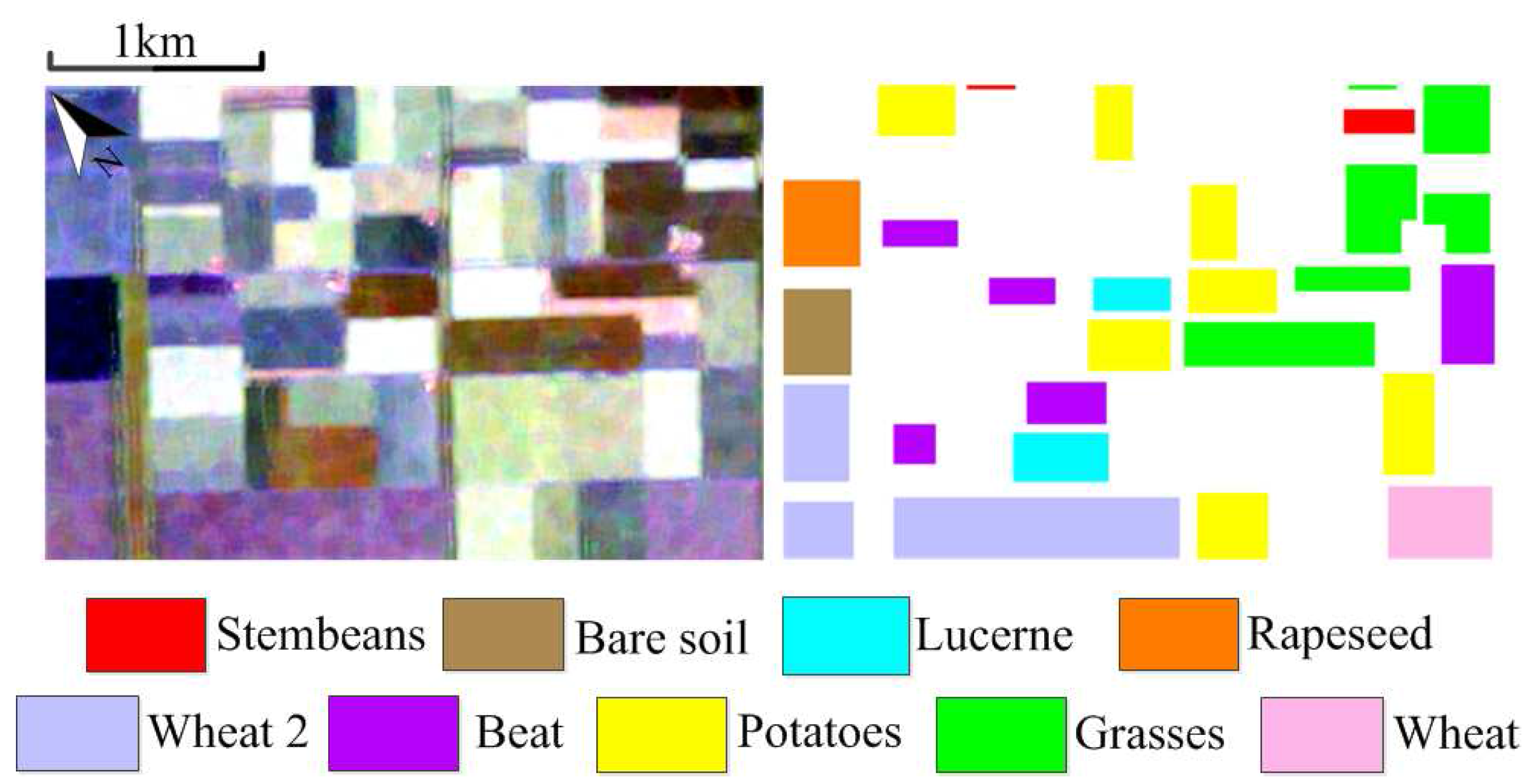
- Dataset 3: The third dataset is one subimage from the well-known AIRSAR L-Band fully polarimetric data shown in Figure 3. It was acquired by the Netherlands on 16 August 1989 during the MAESTRO-1 Campaign. It owns recognized ground truth to test the natural vegetation and land covers. In this subimage, it covers 9 different crops containing: stembeans, bare soil, lucerne, rapeseed, wheat 2, beat, potatoes, grasses, wheat. Those regularization parameters utilized here are set as .
4.2. Analysis of Reduced Dimensions
For testing the performance of the subspace clustering methods, we select RADARSAT-2 Xi’an dataset to verify the effectiveness of features in different reduced low dimensions. We employ different techniques to uniformly reduce high dimensional data into five dimensions for land cover classification. Those typical low dimensions contain 1, 7, 13, 19, and 25. Each of them differs by 6 dimensions. We show OA and Kappa coefficient classification bar chart in Figure 4.
The low dimensional projection number is an important parameter in dimensional reduction techniques. It can be seen that the performances of OA and kappa coefficient increase with the dimension increasing in a certain extent. When the dimensions exceed 13, there is no improvement in performance. This is because, when the dimension exceeded a specific value, the components in PCA related algorithms would obtain enough discriminative information. The features extracted from the subspace clustering based methods also achieve projection information. It can be assumed that the intrinsic dimension of PolSAR data is less than 13 and greater than 7. Nevertheless, the OA in subspace clustering methods have reached 88%, and is better than LE and PCA contrast methods. This means that, under a proper constraint, the sparsity and manifold regularized would preferably mine the polarimetric data information and obtain an effective projection matrix.
4.3. Quantitative Evaluation and Classification Result
In this part, the quantization and visualization classification performance are tested in west Xi’an data and RADARSAT-2 Flevoland data. In order to prove the universality, the kNN algorithm is utilized to classify the low dimension features. The number of the supervised samples is selected related to the number of oversegmentation resolution units. In the two datasets, the training samples used 20–40 samples per class. The low dimensional projection number is set to 9 for those two datasets.
The experiment results of west Xi’an data are shown in Figure 5 and Table 1. In this figure, the LE algorithm shows the worst visualization classification result. From the black rectangle area, it misclassifies lots of buildings as water region, and performs the lowest quantitation result in OA, AA, and kappa coefficient. Compared to subspace clustering based algorithms, PCA and KPCA do not show strong visual inferiority, because the PolSAR dataset has a few categories. Moreover, there is not much difference between subspace clustering based methods in the visualization performance. Compared to contrast methods, features form the proposed methods are sensitive to water and building regions. From the classification indicators of subspace clustering methods, the OA of the water region is almost greater than 79% and Kappa coefficient better than 0.80. This demonstrated that the proposed methods have advantages in quantitation and visualization classification for local regions and the whole area in PolSAR images.
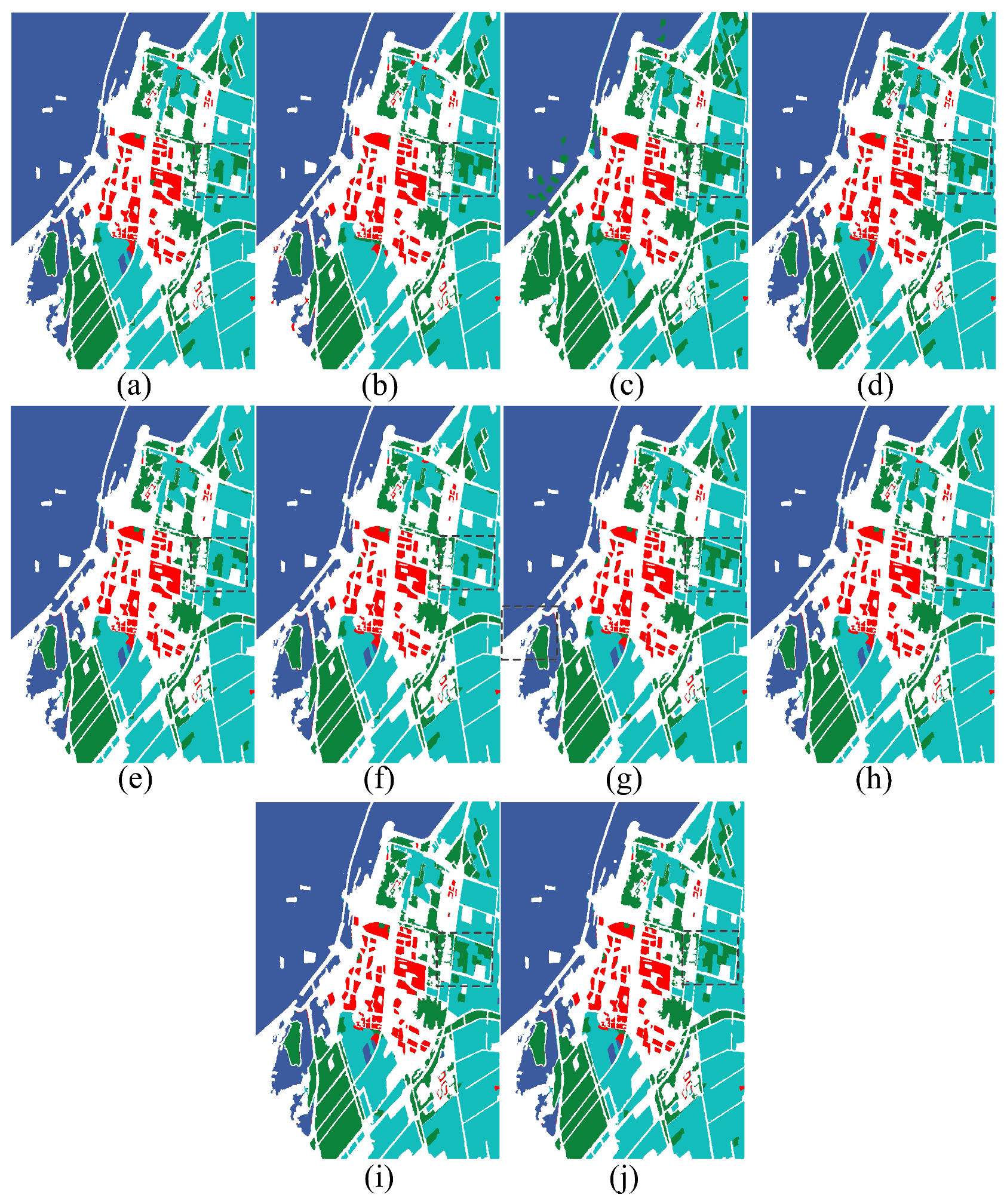
Figure 6 and Table 2 show the classification result of RADARSAT-2 Flevoland dataset. Similar to west Xi’an dataset, all techniques are not sensitive to grass region that always be misclassified as wood regions as shown in the black rectangle. PCA and subspace clustering based algorithms show better classification performance, OA all greater than 90%. Since polarimetric data cannot construct a whole connected graph, the LE algorithm presents the worst result and it is not suitable for the dimensional reduction of PolSAR features.
From the sparse subspace algorithms regularized form the different manifold constraints, it is possible to observe that there exist some differences in LapLRSC_ED, LapLRSC_MulG, and LapLRSC_SRW. This is because the method of constructing the manifold graph regularization influences the feature extraction performance in the proposed methods. In three of the manifold regularized algorithms, LapLRSC_ED achieves the best classification result. Its OA exceeds 97% and kappa coefficients is greater than 0.95, which precede the LapLRSC_ED and LapLRSC_MulG. This shows that the modalities division of multiple features in multi-graph construction is not reasonable. For different dataries and machine learning algorithms, the statistical information derived manifold sometimes also shows a poor performance. Then the manifold graph terms in subspace clustering based method can provide information from different perspectives reflecting the PolSAR data property.
4.4. The Contrasts of Kernelized Methods
For many subspace clustering based methods, it may not be suitable to directly project original features into low dimensional space. Then it is necessary to test the non-linearity property in the PolSAR feature. We employ the kernel function to transform the data into a high dimensional feature space. It can make the non-linear data linearly separable and in same distribution. Then a positive semidefinite kernel Gram matrix is denoted as:
In this paper, the polynomial kernels are utilized to transform the feature matrix to a Hilbert space . We transform the SSC, LRSC, LapLSSC algorithms into the kernelized version as NLLRSC, NLSSC, NLLapLSSC with parameters and . The original feature are projected into a 3-dimnensonal space by linear and nonlinear subspace clustering based methods. Classification performances are reported in Table 3 and Figure 7.
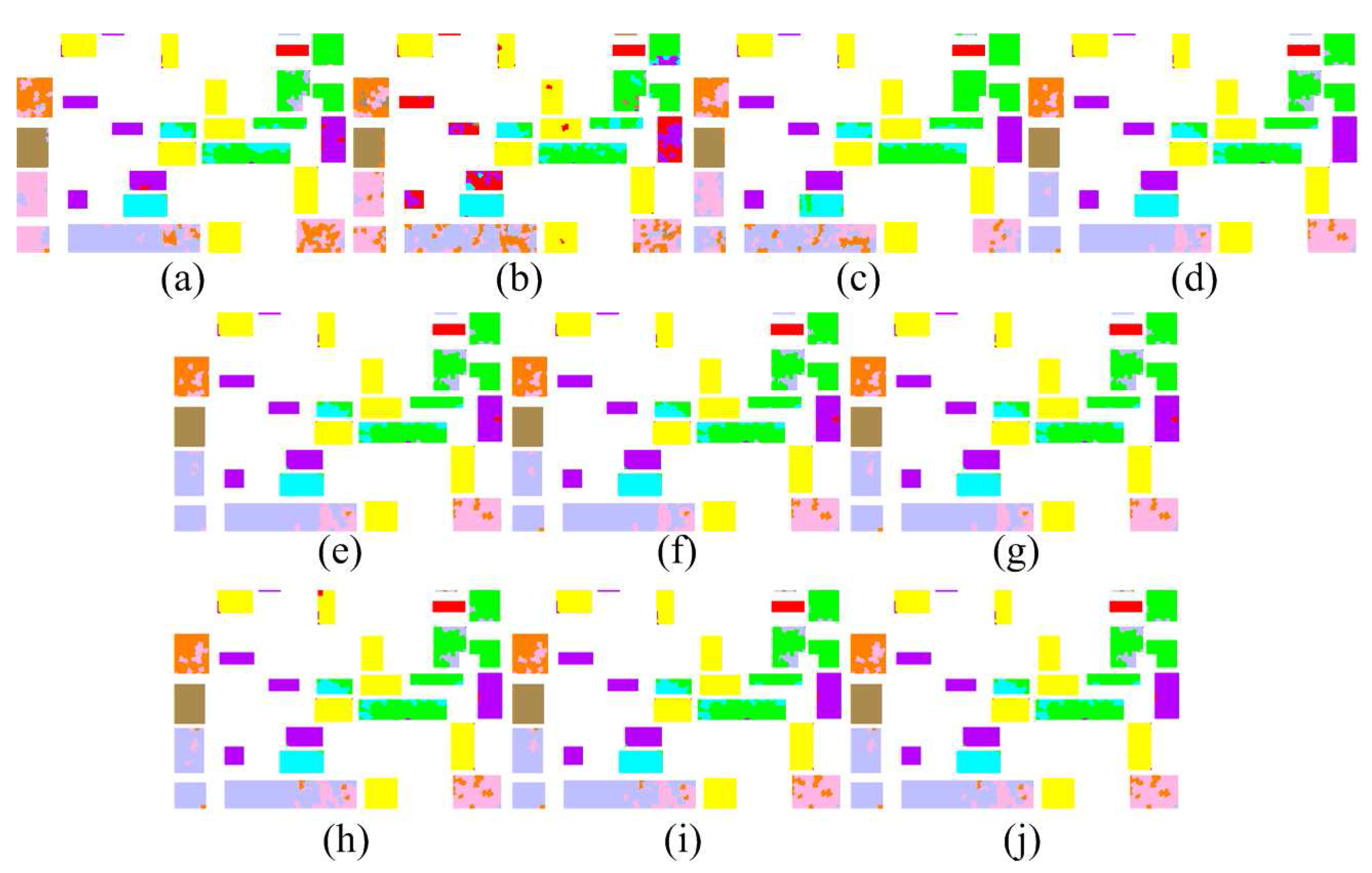
From the classification results, the proposed methods can achieve better performance with more categories. The linear subspace algorithms show higher quantitative results that OA is more than 90% and Kappa coefficient exceeds 0.90. Compared to PCA, LE, and KPCA, they have great improvement in classification. For the regions with low discrimination, the contrast methods have clear disadvantages in wheat and bare oil. Especially for PCA related methods, OA does not reach 60%, and those methods present some confusion in classification images. Some subspace clustering based methods show little difference and all of them present superior visualization and quantitation results. However, kernelized methods do not perform well in the PolSAR dataset, because the low-rank and sparse representation can capture the compact data structure enough in the linear model. The unnecessary nonlinear operations will reduce the sensitivity of model to PolSAR data. It may not improve the model capacity to the specific data. Generally, the proposed methods could obtain discriminative features for the subsequent classification.
5. Discussion
For PolSAR Classification, features extraction and classifier design are two significant steps in machine learning methods. In the proposed method, we construct some combinations of sparsity, low rank, and manifold graph constraints to investigate the intrinsic property of PolSAR data. In order to improve the classification performance, the projection matrix is computed to extract discriminative information by fusing the multi-modal features. The experiments analyze the visualization and quantization results and demonstrate that the features extracted from the subspace clustering based methods are superior to other contrasting methods.
The performance varies from 1D to 25D, the OA and Kappa coefficients are shown in Figure 4. This shows that the proposed algorithm achieves more discriminative features in different dimensions constrained by corresponding terms from the multi-modal observations. There is not too much difference in the performance of the subspace clustering based algorithms. This is due to the intrinsic dimension near to the number of free variables in the coherency matrix of PolSAR data.
In order to demonstrate the effectiveness of the subspace clustering methods, the quantization and visualization performance are simultaneously evaluated. In Figure 5, the subspace clustering methods have the capacity to identify the water region in the black rectangle, and Table 1 presents the same performance as well. We also see from Figure 6 and Table 2 that it is important to explore the geometry structure of data. After being regularized by manifold graph terms, LapLRSC_SRW, LapLRSC_ED, and LapLRSC_MulG can exploit the geometry structure from different perspectives. They can actually reflect the data property in a subspace clustering framework.
The subspace clustering algorithms are also kernelized to a high-dimensional Hilbert space, which is utilized to test the performance of nonlinear version of subspace clustering algorithms in PolSAR data. With a polynomial kernel, NLLRR, NLSSC, and NLLapLSSC is formed. However, those nonlinear methods do not perform well in a PolSAR dataset because the proposed methods have enough capacity to capture the PolSAR data structure. The OA and Kappa coefficients of proposed methods exceed 90% and 0.90 respectively. This is vastly superior to the contrast methods in Table 3. This demonstrates that sparse constrained algorithms can detect the intrinsic samples’ property, especially if the processed PolSAR dataset has more categories. In summary, those subspace clustering methods can obtain an effective projection matrix to achieve more discriminative features for the subsequent classification.
6. Conclusions
In this paper, we present algorithms based on subspace clustering methods to investigate the intrinsic structure of PolSAR data. In this proposed framework, the sparsity term aims at searching for a few of points from each same subspace. Low rank and manifold terms are utilized to detect the local and global geometry structure of data. First, some comprehensive features are extracted from PolSAR data. They mainly cover some physical information and parameters from target decompositions, which can be realized by PolSARpro5.0 software. Secondly, the projection matrix and affinity matrix can be obtained from framework constrained by different combinations of those terms. Finally, experiments on three datasets from airborne and spaceborne platforms demonstrate that the features from subspace clustering method outperform to several contrast methods. Overall, the projection matrix from the proposed algorithms under the constrained of those terms can extract more promising features for the subsequent PolSAR land cover classification. In future work, we mainly focus on extracting comprehensive feature from the PolSAR data, and constructing the deep leaning structure models for exploiting more abstract features. This requires us to develop a parallel structure to improve the calculation efficiency of the eigen-value calculation in algorithms.
Acknowledgments
The authors would like to thanks the helpers in reviewing and editing. Especially, we thanks for the works about subspace clustering from Vishal M. Patel and Ehsan Elhamifar, which give us motivations to explore the PolSAR data. The codes of SSC, LRSC, and LRSSC related algorithms can be obtained from their homepage [59,60]. This work was supported in part by the National Natural Science Foundation of China under Grant No. 61671350; the Project supported the Foundation for Innovative Research Groups of the National Natural Science Foundation of China under Grant No. 61621005; and the Major Research Plan of the National Natural Science Foundation of China under Grant No. 91438201. [grant number 61671350, 61621005, and 91438201].
Author Contributions
Bo Ren theoretically proposed this original method and test on PolSAR data. Jin Zhao gave the mathematically help in formula derivation. Biao Hou and Licheng Jiao gave some suggestions.
Conflicts of Interest
The authors declare no conflict of interest.
Abbreviations
The following abbreviations are used in this manuscript:
| PolSAR | Polarimetric synthetic aperture image |
| ICA | Independent component analysis |
| SSC | Sparse subspace clustering |
| LRSC | Low rank subspace clustering |
| LRSSC | Low rank sparse subspace clustering |
| LLRSC | Laplacian regularized low rank subspace clustering |
| SP | Sparse representation |
| LLR | Low rank representation |
| MR | Manifold regularizations |
| ADMM | Alternative direction method of multipliers |
| SRW | Symmetry revised Wishart |
| LapLRR | Laplacian regularized low rank representation |
| LapLRSC-ED | Euclidean distance based LapLRSC |
| LapLRSC-SRW | SRW distance based LapLRSC |
| LapLRSC-MulG | Multi graph model based LapLRSC |
| LapLSSC | Laplacian manifold regularized low-rank sparse subspace |
| NLSSC | Nonlinear Sparse subspace clustering |
| NLLSC | Nonlinear Low rank subspace clustering |
| NLLapLSSC | Nonlinear Laplacian regularized low rank representation |
| AA | Average accuracy |
| OA | Overall accuracy |
| NN | Nearest Neighbor |
References
- Krogager, E. New decomposition of the radar target scattering matrix. Electron. Lett. 1990, 26, 1525–1527. [Google Scholar] [CrossRef]
- Cloude, S.R. Uniqueness of target decomposition theorems in radar polarimetry. In Direct and Inverse Methods in Radar Polarimetry; Springer: Dordrecht, The Netherlands, 1992; pp. 267–296. [Google Scholar]
- Vanzyl, J.J. Application of Cloude’s target decomposition theorem to polarimetric imaging radar data. In Proceedings of the SPIE—The International Society for Optical Engineering, San Diego, CA, USA, 12 February 1993. [Google Scholar]
- Freeman, A.; Durden, S.L. A three-component scattering model for polarimetric SAR data. IEEE Trans. Geosci. Remote Sens. 1998, 36, 963–973. [Google Scholar] [CrossRef]
- Yamaguchi, Y.; Moriyama, T.; Ishido, M.; Yamada, H. Four-component scattering model for polarimetric SAR image decomposition. IEEE Trans. Geosci. Remote Sens. 2005, 43, 1699–1706. [Google Scholar] [CrossRef]
- Lee, J.S.; Grunes, M.R.; Kwok, R. Classification of multi-look polarimetric SAR imagery based on complex Wishart distribution. Int. J. Remote Sens. 1994, 15, 2299–2311. [Google Scholar] [CrossRef]
- Lee, J.S.; Grunes, M.R.; Ainsworth, T.L.; Du, L.J.; Schuler, D.L.; Cloude, S.R. Unsupervised classification using polarimetric decomposition and the complex Wishart classifier. IEEE Trans. Geosci. Remote Sens. 1999, 37, 2249–2258. [Google Scholar]
- Tu, S.T.; Chen, J.Y.; Yang, W.; Sun, H. Laplacian eigenmaps-based polarimetric dimensionality reduction for SAR image classification. IEEE Trans. Geosci. Remote Sens. 2012, 50, 170–179. [Google Scholar] [CrossRef]
- Zhang, L.; Sun, L.; Zou, B.; Moon, W.M. Fully polarimetric SAR image classification via sparse representation and polarimetric features. IEEE J. Sel. Top. Appl. Earth Obs. Remote Sens. 2015, 8, 3923–3932. [Google Scholar] [CrossRef]
- Song, H.; Yang, W.; Zhong, N.; Xu, X. Unsupervised classification of PolSAR imagery via kernel sparse subspace clustering. IEEE Geosci. Remote Sens. Lett. 2016, 13, 1487–1491. [Google Scholar] [CrossRef]
- Chen, L.; Yang, W.; Liu, Y.; Sun, H. Feature evaluation and selection for polarimetric SAR image classification. In Proceedings of the 2010 IEEE 10th International Conference on Signal Processing (ICSP), Beijing, China, 22–28 October 2010; pp. 2202–2205. [Google Scholar]
- Zou, T.; Yang, W.; Dai, D.; Sun, H. Polarimetric SAR image classification using multifeatures combination and extremely randomized clustering forests. EURASIP J. Adv. Signal Process. 2010, 2010, 4. [Google Scholar] [CrossRef]
- Shi, L.; Zhang, L.; Yang, J.; Zhang, L.; Li, P. Supervised graph embedding for polarimetric SAR image classification. IEEE Geosci. Remote Sens. Lett. 2013, 10, 216–220. [Google Scholar] [CrossRef]
- Loosvelt, L.; Peters, J.; Skriver, H.; De Baets, B.; Verhoest, N.E. Impact of reducing polarimetric SAR input on the uncertainty of crop classifications based on the random forests algorithm. IEEE Trans. Geosci. Remote Sens. 2012, 50, 4185–4200. [Google Scholar] [CrossRef]
- Tao, M.; Zhou, F.; Liu, Y.; Zhang, Z. Tensorial independent component analysis-based feature extraction for polarimetric SAR data classification. IEEE Trans. Geosci. Remote Sens. 2015, 53, 2481–2495. [Google Scholar] [CrossRef]
- Ersahin, K.; Cumming, I.G.; Ward, R.K. Segmentation and classification of polarimetric SAR data using spectral graph partitioning. IEEE Trans. Geosci. Remote Sens. 2010, 48, 164–174. [Google Scholar] [CrossRef]
- Hou, B.; Kou, H.; Jiao, L. Classification of polarimetric SAR images using multilayer autoencoders and superpixels. IEEE J. Sel. Top. Appl. Earth Obs. Remote Sens. 2016, 9, 3072–3081. [Google Scholar] [CrossRef]
- Licciardi, G.; Avezzano, R.G.; Del Frate, F.; Schiavon, G.; Chanussot, J. A novel approach to polarimetric SAR data processing based on Nonlinear PCA. Pattern Recognit. 2014, 47, 1953–1967. [Google Scholar] [CrossRef]
- Tannous, O.; Kasilingam, D. Independent component analysis of polarimetric SAR data for separating ground and vegetation components. In Proceedings of the 2009 IEEE International Geoscience and Remote Sensing Symposium (IGARSS), Cape Town, South Africa, 12–17 July 2009; Volume 4, pp. IV-93–IV-96. [Google Scholar]
- Totir, F.; Vasile, G.; Gay, M.; Anton, L.; Ilie, G. ICA-based information extraction method for PolSAR images. In Proceedings of the 2010 8th International Conference on Communications (COMM), Bucharest, Romania, 10–12 June 2010; pp. 149–152. [Google Scholar]
- Ainsworth, T.L.; Lee, J.S. Polarimetric SAR image classification-exploiting optimal variables derived from multiple-image datasets. In Proceedings of the 2004 IGARSS’04 IEEE International Geoscience and Remote Sensing Symposium, Anchorage, AK, USA, 20–24 September 2004; Volume 1. [Google Scholar]
- Elhamifar, E.; Vidal, R. Sparse subspace clustering: Algorithm, theory, and applications. IEEE Trans. Pattern Anal. Mach. Intell. 2013, 35, 2765–2781. [Google Scholar] [CrossRef] [PubMed]
- Patel, V.M.; Van Nguyen, H.; Vidal, R. Latent space sparse and low-rank subspace clustering. IEEE J. Sel. Top. Signal Process. 2015, 9, 691–701. [Google Scholar] [CrossRef]
- Ho, J.; Yang, M.H.; Lim, J.; Lee, K.C.; Kriegman, D. Clustering appearances of objects under varying illumination conditions. In Proceedings of the 2003 IEEE Computer Society Conference on Computer Vision and Pattern Recognition, Madison, WI, USA, 18–20 June 2003; Volume 1, pp. I-11–I-18. [Google Scholar]
- Gear, C.W. Multibody grouping from motion images. Int. J. Comput. Vis. 1998, 29, 133–150. [Google Scholar] [CrossRef]
- Tipping, M.E.; Bishop, C.M. Mixtures of probabilistic principal component analyzers. Neural Comput. 1999, 11, 443–482. [Google Scholar] [CrossRef] [PubMed]
- Sugaya, Y.; Kanatani, K.I. Geometric Structure of Degeneracy for Multi-Body Motion Segmentation; ECCV Workshop SMVP; Springer: New York, NY, USA, 2004; pp. 13–25. [Google Scholar]
- Yan, J.; Pollefeys, M. A general framework for motion segmentation: Independent, articulated, rigid, non-rigid, degenerate and non-degenerate. In European Conference on Computer Vision; Springer: New York, NY, USA, 2006; pp. 94–106. [Google Scholar]
- Goh, A.; Vidal, R. Segmenting motions of different types by unsupervised manifold clustering. In Proceedings of the 2007 CVPR’07 IEEE Conference on Computer Vision and Pattern Recognition, Minneapolis, MN, USA, 17–22 June 2007; pp. 1–6. [Google Scholar]
- Elhamifar, E.; Vidal, R. Clustering disjoint subspaces via sparse representation. In Proceedings of the 2010 IEEE International Conference on Acoustics Speech and Signal Processing (ICASSP), Dallas, TX, USA, 14–19 March 2010; pp. 1926–1929. [Google Scholar]
- Soltanolkotabi, M.; Candes, E.J. A geometric analysis of subspace clustering with outliers. Ann. Stat. 2012, 40, 2195–2238. [Google Scholar] [CrossRef]
- Vidal, R.; Favaro, P. Low rank subspace clustering (LRSC). Pattern Recognit. Lett. 2014, 43, 47–61. [Google Scholar] [CrossRef]
- Liu, G.; Lin, Z.; Yan, S.; Sun, J.; Yu, Y.; Ma, Y. Robust recovery of subspace structures by low-rank representation. IEEE Trans. Pattern Anal. Mach. Intell. 2013, 35, 171–184. [Google Scholar] [CrossRef] [PubMed]
- Wang, Y.X.; Xu, H.; Leng, C. Provable Subspace Clustering: When LRR Meets SSC; Advances in Neural Information Processing Systems: Cambridge, MA, USA, 2013; pp. 64–72. [Google Scholar]
- Song, Y.; Wu, Y. Laplacian regularized low rank subspace clustering. arXiv, 2016; arXiv:1610.07488. [Google Scholar]
- Van Zyl, J.J. Unsupervised classification of scattering behavior using radar polarimetry data. IEEE Trans. Geosci. Remote Sens. 1989, 27, 36–45. [Google Scholar] [CrossRef]
- Cloude, S.R. Target decomposition theorems in radar scattering. Electron. Lett. 1985, 21, 22–24. [Google Scholar] [CrossRef]
- Cloude, S.R.; Pottier, E. An entropy based classification scheme for land applications of polarimetric SAR. IEEE Trans. Geosci. Remote Sens. 1997, 35, 68–78. [Google Scholar] [CrossRef]
- Touzi, R. Target scattering decomposition in terms of roll-invariant target parameters. IEEE Trans. Geosci. Remote Sens. 2007, 45, 73–84. [Google Scholar] [CrossRef]
- ESA. PolSARPro V5.0. Available online: http://earth.esa.int/polsarpro (accessed on 1 March 2018).
- You, C.; Vidal, R. Subspace-sparse representation. arXiv, 2015; arXiv:1507.01307. [Google Scholar]
- Liu, J.; Chen, Y.; Zhang, J.; Xu, Z. Enhancing low-rank subspace clustering by manifold regularization. IEEE Trans. Image Process. 2014, 23, 4022–4030. [Google Scholar] [CrossRef] [PubMed]
- Fazel, M. Matrix Rank Minimization with Applications. Ph.D. Thesis, Stanford University, Stanford, CA, USA, 2002. [Google Scholar]
- Boyd, S.; Parikh, N.; Chu, E.; Peleato, B.; Eckstein, J. Distributed optimization and statistical learning via the alternating direction method of multipliers. Found. Trends Mach. Learn. 2011, 3, 1–122. [Google Scholar] [CrossRef]
- Seung, H.S.; Lee, D.D. The manifold ways of perception. Science 2000, 290, 2268–2269. [Google Scholar] [CrossRef] [PubMed]
- He, X.; Niyogi, P. Locality Preserving Projections. Adv. Neural Inf. Process. Syst. 2003, 16, 186–197. [Google Scholar]
- Ren, X.; Malik, J. Learning a classification model for segmentation. Proc. Int. Conf. Comput. Vis. 2003, 2, 10–17. [Google Scholar]
- Shi, J.; Malik, J. Normalized cuts and image segmentation. IEEE Trans. Pattern Anal. Mach. Intell. 2000, 22, 888–905. [Google Scholar]
- Anfinsen, S.N.; Jenssen, R.; Eltoft, T. Spectral clustering of polarimetric SAR data with Wishart-derived distance measures. In Proc. POLinSAR 2007, 7, 1–9. [Google Scholar]
- Dong, X.; Frossard, P.; Vandergheynst, P.; Nefedov, N. Clustering on multi-layer graphs via subspace analysis on Grassmann manifolds. IEEE Trans. Signal Process. 2014, 62, 905–918. [Google Scholar] [CrossRef]
- Von Luxburg, U. A tutorial on spectral clustering. Stat. Comput. 2007, 17, 395–416. [Google Scholar] [CrossRef]
- Zhang, L.; Zhang, Q.; Zhang, L.; Tao, D.; Huang, X.; Du, B. Ensemble manifold regularized sparse low-rank approximation for multiview feature embedding. Pattern Recognit. 2015, 48, 3102–3112. [Google Scholar] [CrossRef]
- Cai, D.; He, X.; Han, J.; Huang, T.S. Graph regularized nonnegative matrix factorization for data representation. IEEE Trans. Pattern Anal. Mach. Intell. 2011, 33, 1548–1560. [Google Scholar] [PubMed]
- Wang, C.; He, X.; Bu, J.; Chen, Z.; Chen, C.; Guan, Z. Image representation using Laplacian regularized nonnegative tensor factorization. Pattern Recognit. 2011, 44, 2516–2526. [Google Scholar] [CrossRef]
- Ren, B.; Hou, B.; Zhao, J.; Jiao, L. Unsupervised classification of polarimetirc SAR image via improved manifold regularized low-rank representation with multiple features. IEEE J. Sel. Top. Appl. Earth Obs. Remote Sens. 2017, 10, 580–595. [Google Scholar] [CrossRef]
- Patel, V.M.; Vidal, R. Kernel sparse subspace clustering. In Proceedings of the 2014 IEEE International Conference on Image Processing (ICIP), Paris, France, 27–30 October 2014; pp. 2849–2853. [Google Scholar]
- Lee, J.S. Digital image enhancement and noise filtering by use of local statistics. IEEE Trans. Pattern Anal. Mach. Intell. 1980, PAMI-2, 165–168. [Google Scholar] [CrossRef]
- Lee, J.S. Speckle suppression and analysis for synthetic aperture radar images. Opt. Eng. 1986, 25, 255636. [Google Scholar] [CrossRef]
- Patel, V.M. Homepage. Available online: http://www.ccs.neu.edu/home/eelhami/codes.htm (accessed on 1 March 2018).
- Elhamifar, E. Homepage. Available online: http://www.umiacs.umd.edu/~pvishalm/Research.html (accessed on 1 March 2018).
Figure 1.
RADARSAT-2 Xi’an dataset.

Figure 2.
RADARSAT-2 Flevoland dataset.

Figure 3.
AIRSAR Flevoland dataset.

Figure 4.
Classification performance variation from dimensions in Xi’an dataset.
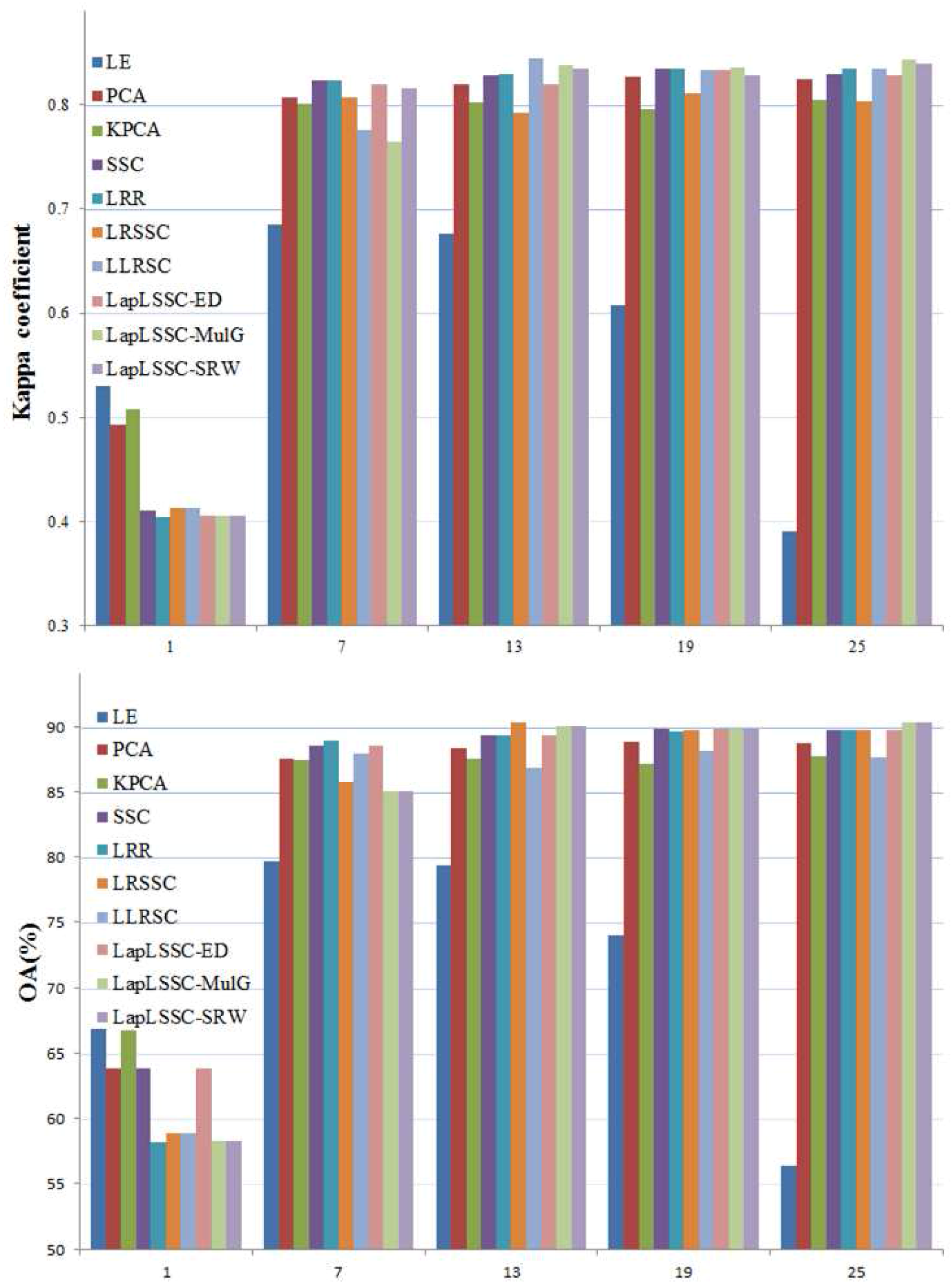
Figure 5.
RADARSAT-2 West Xi’an dataset classification result. (a) PCA; (b) KPCA; (c) LE; (d) SSC; (e) LRSC; (f) LRSSC; (g) LapLSSC; (h) LapLRSC_ED; (i) LapLRSC_SRW; (j) LapLRSC_MulG.
Figure 5.
RADARSAT-2 West Xi’an dataset classification result. (a) PCA; (b) KPCA; (c) LE; (d) SSC; (e) LRSC; (f) LRSSC; (g) LapLSSC; (h) LapLRSC_ED; (i) LapLRSC_SRW; (j) LapLRSC_MulG.
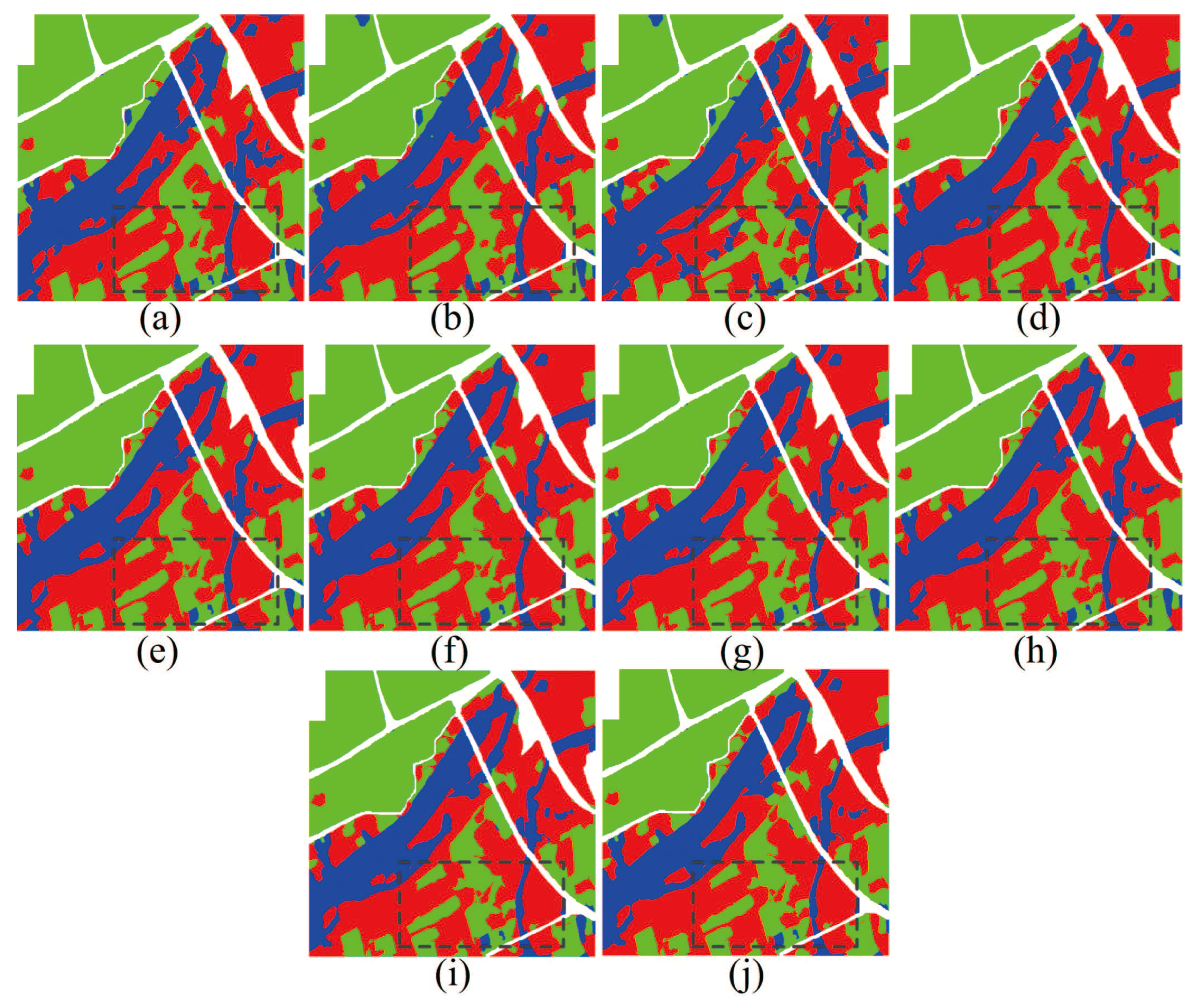
Figure 6.
RADARSAT-2 Flevoland classification result. (a) PCA; (b) KPCA; (c) LE; (d) SSC; (e) LRSC; (f) LRSSC; (g) LapLSSC; (h) LapLRSC_ED; (i) LapLRSC_SRW; (j) LapLRSC_MulG.
Figure 6.
RADARSAT-2 Flevoland classification result. (a) PCA; (b) KPCA; (c) LE; (d) SSC; (e) LRSC; (f) LRSSC; (g) LapLSSC; (h) LapLRSC_ED; (i) LapLRSC_SRW; (j) LapLRSC_MulG.

Figure 7.
AIRSAR Flevoland 3D classification result. (a) PCA ; (b) KPCA; (c) LE; (d) SSC; (e) LRSC; (f) LRSSC; (g) LapLSSC; (h) NLSSC; (i) NLLRR; (j) NLLLR_SCC.
Figure 7.
AIRSAR Flevoland 3D classification result. (a) PCA ; (b) KPCA; (c) LE; (d) SSC; (e) LRSC; (f) LRSSC; (g) LapLSSC; (h) NLSSC; (i) NLLRR; (j) NLLLR_SCC.


Table 1.
RADARSAT-2 Xi’an 9 dimension classification result.
| Algorithms | Grass | Buildings | Water | OA | AA | Kappa |
|---|---|---|---|---|---|---|
| PCA | 96.02 | 97.38 | 73.87 | 85.51 | 89.09 | 0.7729 |
| LE | 97.12 | 95.77 | 70.38 | 83.38 | 87.76 | 0.7418 |
| KPCA | 96.84 | 96.86 | 77.64 | 87.32 | 90.45 | 0.7922 |
| SSC | 96.78 | 96.11 | 79.56 | 88.00 | 90.82 | 0.8092 |
| LRSC | 96.78 | 96.15 | 79.58 | 88.02 | 90.84 | 0.8095 |
| LRSSC | 96.75 | 96.16 | 79.56 | 88.59 | 90.82 | 0.8090 |
| LapLSSC | 96.75 | 96.16 | 79.56 | 88.01 | 90.82 | 0.8093 |
| LapLRSC_ED | 96.78 | 96.16 | 79.58 | 88.61 | 90.84 | 0.8096 |
| LapLRSC_MulG | 96.78 | 96.11 | 79.67 | 88.59 | 90.86 | 0.8099 |
| LapLRSC_SRW | 96.78 | 96.16 | 79.51 | 88.69 | 90.82 | 0.8091 |
Table 2.
RADARSAT-2 Flevoland 9 dimension classification result.
| Algorithms | Water | Grass | Wood | Building | OA | AA | Kappa |
|---|---|---|---|---|---|---|---|
| PCA | 98.35 | 92.78 | 98.77 | 96.30 | 96.69 | 96.55 | 0.9490 |
| LE | 99.51 | 81.88 | 85.17 | 97.65 | 86.92 | 91.05 | 0.8106 |
| KPCA | 98.60 | 92.20 | 98.82 | 98.01 | 96.29 | 96.91 | 0.9445 |
| SSC | 98.52 | 92.08 | 99.15 | 96.57 | 96.29 | 96.58 | 0.9444 |
| LRSC | 98.60 | 93.98 | 99.15 | 97.02 | 97.03 | 97.19 | 0.9554 |
| LRSSC | 98.63 | 94.17 | 99.17 | 97.02 | 97.12 | 97.25 | 0.9567 |
| LapLSSC | 98.51 | 91.89 | 99.15 | 97.14 | 96.25 | 96.67 | 0.9438 |
| LapLRSC_ED | 98.61 | 94.10 | 99.17 | 96.91 | 97.08 | 97.20 | 0.9561 |
| LapLRSC_MulG | 98.52 | 91.97 | 99.15 | 97.14 | 96.28 | 96.69 | 0.9443 |
| LapLRSC_SRW | 98.56 | 92.35 | 99.15 | 97.01 | 96.42 | 96.77 | 0.9463 |
Table 3.
AIRSAR Flevoland 3D classification result
| Algorithms | Potato | Wheat | Grass | Beat | Wheat 2 | Lucer Ne | Rapese Ed | Bare Soil | Stem beans | OA | AA | Kappa |
|---|---|---|---|---|---|---|---|---|---|---|---|---|
| PCA | 87.63 | 81.64 | 98.18 | 95.62 | 56.73 | 88.89 | 72.23 | 50.87 | 99.50 | 80.49 | 81.25 | 0.7966 |
| LE | 84.84 | 92.21 | 98.10 | 99.48 | 55.41 | 88.64 | 69.08 | 78.59 | 99.53 | 84.10 | 85.10 | 0.8336 |
| KPCA | 88.99 | 77.54 | 94.13 | 33.86 | 43.81 | 100.0 | 63.52 | 57.32 | 97.90 | 69.42 | 73.01 | 0.6813 |
| SSC | 84.77 | 83.91 | 99.92 | 99.55 | 86.38 | 88.64 | 82.49 | 86.27 | 99.50 | 90.70 | 90.16 | 0.9030 |
| LRSC | 86.13 | 83.91 | 99.92 | 98.61 | 85.86 | 88.89 | 82.49 | 87.56 | 99.50 | 90.64 | 90.32 | 0.9023 |
| LRSSC | 84.77 | 83.97 | 99.92 | 98.61 | 86.38 | 88.89 | 82.49 | 86.27 | 99.50 | 90.61 | 90.09 | 0.9020 |
| LapLSSC | 84.77 | 83.97 | 99.92 | 98.61 | 86.73 | 88.89 | 82.49 | 86.27 | 99.50 | 90.69 | 90.13 | 0.9029 |
| NLLapLSSC | 87.22 | 84.32 | 99.92 | 99.16 | 83.00 | 88.89 | 78.75 | 81.24 | 99.46 | 89.61 | 89.11 | 0.8916 |
| NLSSC | 87.22 | 84.20 | 99.92 | 99.16 | 82.81 | 88.89 | 80.22 | 81.24 | 98.94 | 89.50 | 89.18 | 0.8905 |
| NLLRR | 87.22 | 84.32 | 99.92 | 99.16 | 83.00 | 88.89 | 80.15 | 81.24 | 99.46 | 89.68 | 89.26 | 0.8923 |
© 2018 by the authors. Licensee MDPI, Basel, Switzerland. This article is an open access article distributed under the terms and conditions of the Creative Commons Attribution (CC BY) license (http://creativecommons.org/licenses/by/4.0/).
Share and Cite
MDPI and ACS Style
Ren, B.; Hou, B.; Zhao, J.; Jiao, L. Sparse Subspace Clustering-Based Feature Extraction for PolSAR Imagery Classification. Remote Sens. 2018, 10, 391. https://doi.org/10.3390/rs10030391
AMA Style
Ren B, Hou B, Zhao J, Jiao L. Sparse Subspace Clustering-Based Feature Extraction for PolSAR Imagery Classification. Remote Sensing. 2018; 10(3):391. https://doi.org/10.3390/rs10030391
Chicago/Turabian StyleRen, Bo, Biao Hou, Jin Zhao, and Licheng Jiao. 2018. "Sparse Subspace Clustering-Based Feature Extraction for PolSAR Imagery Classification" Remote Sensing 10, no. 3: 391. https://doi.org/10.3390/rs10030391
Note that from the first issue of 2016, this journal uses article numbers instead of page numbers. See further details here.