Impact of Sea Ice Drift Retrieval Errors, Discretization and Grid Type on Calculations of Ice Deformation


1
The Alfred Wegener Institute, Helmholtz Centre for Polar and Marine Research, Bussestraße 24, 27570 Bremerhaven, Germany
2
Center for Integrated Remote Sensing and Forecasting for Arctic Operations, Arctic University of Norway, Sykehusvegen 21, 9019 Tromsø, Norway
*
Author to whom correspondence should be addressed.
Remote Sens. 2018, 10(3), 393; https://doi.org/10.3390/rs10030393
Submission received: 6 February 2018
/
Revised: 27 February 2018
/
Accepted: 2 March 2018
/
Published: 3 March 2018
(This article belongs to the Section Ocean Remote Sensing)
Abstract
:We studied two issues to be considered in the calculation of parameters characterizing sea ice deformation: the effect of uncertainties in an automatically retrieved sea ice drift field, and the influence of the type of drift vector grid. Sea ice deformation changes the local ice mass balance and the interaction between atmosphere, ice, and ocean, and constitutes a hazard to marine traffic and operations. Due to numerical effects, the results of deformation retrievals may predict, e.g., openings and closings of the ice cover that do not exist in reality. We focus specifically on fields of ice drift obtained from synthetic aperture radar (SAR) imagery and analyze the Propagated Drift Retrieval Error (PDRE) and the Boundary Definition Error (BDE). From the theory of error propagation, the PDRE for the calculated deformation parameters can be estimated. To quantify the BDE, we devise five different grid types and compare theoretical expectation and numerical results for different deformation parameters assuming three scenarios: pure divergence, pure shear, and a mixture of both. Our findings for both sources of error help to set up optimal deformation retrieval schemes and are also useful for other applications working with vector fields and scalar parameters derived therefrom.
1. Introduction
The deformation of sea ice is a key process in sea ice dynamics due to its significant effect on ice production, ice thickness evolution, ice decay, and melting. Deformed sea ice is a potential hazard for logistical operations in the Polar Regions. Sea ice is deformed by mechanical forces generated by wind, ocean currents, internal ice stress, and blocking effects at obstacles such as coastlines, islands, or icebergs. Satellites equipped with, for example, optical scanners or imaging radars can be used to monitor sea ice deformation over regions of smaller and larger extensions, with different spatial and temporal resolutions. In this paper we focus specifically on the use of synthetic aperture radar (SAR) since this instrument type is not affected by cloud cover and darkness. An overview of the use of SAR for sea ice remote sensing and sea ice properties that need to be considered in this context can be found in, e.g., Dierking [1]. Two methods are established to derive sea ice deformation from SAR images:
For both methods, the detectability of deformation features depends mainly on the spatial resolution of the images, the radar frequency used for image acquisition, and the season (freezing versus melting conditions) [11,12,13]. For the retrieval of ice drift, the temporal stability of ice features is an important criterion [14]. In our work presented here we only consider the application of drift detection algorithms to derive sea ice deformation from SAR images.
Drift detection algorithms provide displacement vectors which are approximated from straight lines between the positions of visible sea ice patterns or single features detected in the sequential SAR images. By taking the time passed between the two acquisitions into account, these displacement vectors can be considered as approximations to the path of the ice drift. For pattern matching, it is a common approach to construct a regular Cartesian grid in which the origins of drift vectors lie on the grid vertices. Since prominent ice features are usually irregularly distributed over a region, the drift vectors retrieved from feature tracking are also irregularly spaced and the vector field is unstructured. The spatial and temporal resolutions of the drift vectors depend on the SAR sensor configuration and the time passed until an area is imaged a second time. The derived sea ice deformation is computed from the invariants of the strain rate tensor, which is a function of the partial derivatives of the retrieved drift field [15]. Errors in the computed deformation parameters arise from uncertainties in magnitude and direction of the drift vectors and as a result of the discretization in a grid. Both sources of errors are treated in this paper. Our results are useful for other applications that retrieve or produce sea ice drift data to derive deformation parameters. This includes drift fields from models predicting sea ice conditions as well as data obtained using other observation methods (e.g., buoy arrays).
- Propagated drift retrieval error (PDRE): Based on the theory of error propagation one can estimate the statistical uncertainties of the deformation parameters caused by the uncertainties of the drift vectors [16]. For characterizing deformation, the three invariants divergence, shear, and vorticity are calculated based on the line integral around the boundary of a predefined grid cell. According to Lindsay and Stern [16], the error of the invariants is proportional to the error in area change caused by erroneous drift vectors. It depends on the number of drift vectors used for the calculation of the line integral, the size of the deformation cell, and the acquisition time gap of the successive SAR images. Lindsay and Stern [16], for example, estimated an error in divergence of 0.005 (0.5%) per day for a drift field given at a spatial resolution of 10 by 10 km and with a time gap between image acquisitions of 3 days (both typical for the RADARSAT Geophysical Processor System, RGPS), assuming a drift detection error of 0.1 km. Here, it should be noticed that the deformation error can be much higher when difficult tracking conditions are present or the temporal and spatial resolution changes. This is addressed in the discussion below.
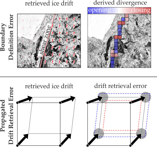
- Boundary definition error (BDE): In the case of sea ice, deformation features often appear as distinct discontinuities in the drift field. Shear zones, e.g., are linear boundaries between ice floes drifting antiparallel relative to one other (see Figure 1). Pressure ridges occur if ice floes move towards each other. Vorticity reflects curvilinear motion and may indicate rotations of single ice floes. With only a few points defining the deformation cell, errors in the computed deformation parameters may be significant because boundaries between different drift zones in the presence of localized deformations such as leads or ridges may not be adequately represented [16]. This results in artificial deformation rates and a loss of invariance [16,17]. Figure 1 shows how the BDE results in artificial opening and closing when a shear zone runs through a regular deformation grid. The BDE may lead to misinterpretations of the derived deformation processes and affect statistics decisively.
The aim of our work is to quantify the uncertainties when deformation is derived from a field of drift vectors retrieved from SAR images on different grids, considering the effect of discretization. To this end we apply analytical expressions based on error propagation (PDRE) and perform numerical experiments (BDE). We present results of these experiments by giving examples and a general overview. Additionally, we visualize a simplified form of the equations expressing the PDRE. Finally, we discuss both error types, their origin, the impact on the computed sea ice deformation, and methods of improvement.
2. Methods
2.1. Deformation Grid and Computation
We obtained the deformation parameters shear, divergence, and vorticity directly from the spatial derivatives of the retrieved drift field:
The derivatives are calculated using the line integral around the boundaries of a grid cell. For this purpose, grids need to be defined, where each grid vertex represents the origin of a drift vector.
The simplest case is implemented as regularly distributed origins of drift vectors on a grid of squares (Q1, Figure 2a). A grid of right-angled triangles can vary in the individual orientation of the triangles (T1 and T2, Figure 3c,d). For spatially irregularly distributed drift vector origins (as in the case of feature tracking), we used paving or triangulation algorithms to create a grid of quadrangles or triangles (Q2 and T3, Figure 2b,e). These algorithms maximize the individual internal angles of the grid cells.
The partial derivatives of the drift vector field are calculated from a line integral, which for discrete values is approximated by using the trapezoidal rule (e.g., ∂u/∂x):
where A is the area of the cell, which is obtained from Gauss’s area formula. The other partial derivatives were determined analogously by the following equations:
2.2. Propagated Drift Retrieval Error
The standard uncertainty of the deformation parameters (vorticity, shear, and divergence) as a result of the drift retrieval uncertainties can be derived using the theory of error propagation. The variances for the velocity gradients ux,, uy, vx, and vy are obtained from calculating the derivatives for A, ui, and yi (e.g., ):
Since we are working in a fixed grid, with the origins of the drift vectors on the vertices, the positions (xi, yi) and the size of the grid cells are known exactly; hence, we can set Ex = 0, Ey = 0, and EA = 0. For the remaining term we obtain
Combining the gradients according to Equation (2) and assuming the same error in the x and y components (Eu = Ev = EU), the variance of divergence calculated for a polygon is
Applying the theory of error propagation for the different deformation parameters (Equations (1)–(4)), the following relationship is obtained for their uncertainties:
In the following sections, the errors of the invariants given above are jointly denoted as “PDRE”. In a grid consisting of squares with sides of length L, the expression for the standard deviation of the invariants is [16]
For right-angled triangles with two equally long legs each of length L, one obtains
where ∆t is the time between the acquisitions of the image pair from which the displacement is retrieved, and the tracking (displacement) error is related to the error of the drift velocity via EU = Etr/∆t. The difficult part is to determine the tracking error Etr. The most commonly applied method to determine this error is a comparison of the automatically retrieved sea ice displacement by using reference data obtained from drifting buoys or from visually tracking ice displacement in an image pair.
2.3. Boundary Definition Error
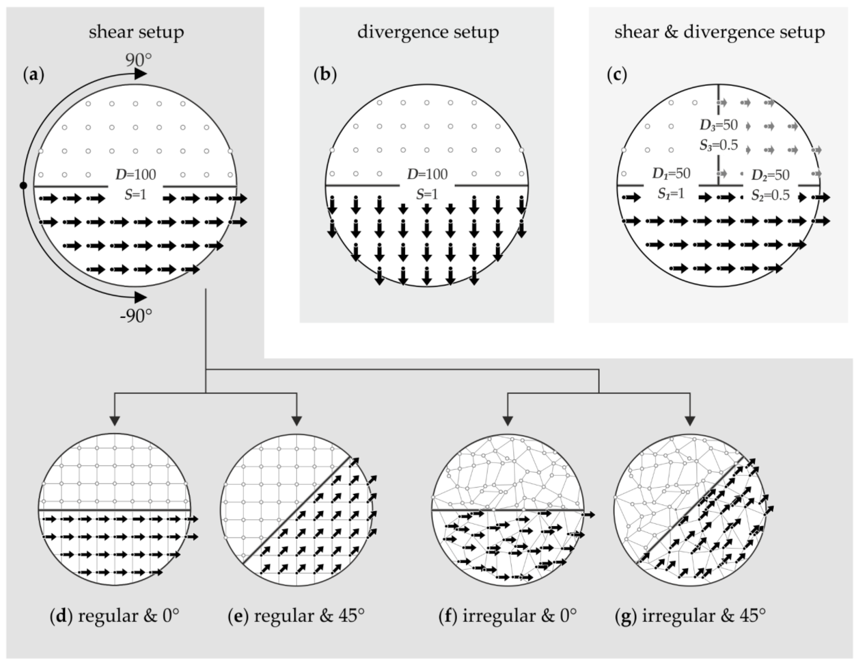
In order to quantify the boundary definition error (BDE) of the computed deformation parameters we performed numerical experiments. We defined three test setups based on simple deformation mechanisms (shear, opening, and a combination of both; Figure 3). The test setups were circularly arranged drift/displacement fields with a diameter of 100 length units and 502 × π vectors (~8000 vectors with components u and v).
Discontinuities in the vector field represent the selected sea ice deformation type (Figure 3). Each test setup comprises two different vector distributions in space, namely regular and irregular. The displacement vector length was set to 0.0 (white), 0.5 (gray), and 1.0 (black) length units L in the various regions separated by a crack (Figure 3). Here, the length unit L is the distance between the adjacent drift vector origins in a regular spatial distribution and correspond to the side length of a squared grid cell.
With the objective to investigate the dependency of the BDE on the angles between the cell boundaries and the discontinuity, we changed the orientation of the discontinuities relative to the x-axis by an angle ϕ in all 15 setups (three mechanisms and five grid layouts). The corresponding drift vectors were rotated by the same angle, whereas the grid vertex positions (i.e., the origins of the vectors) were kept constant. We varied the angle ϕ from 90° to −90° in 1° increments, hence covering the entire possible range of angles.
Note that in some cases the discontinuity has to be separated into different segments. The length of each segment, Dj, and the relative displacement along a corresponding discontinuity segment (denoted as the sliding distance S) are both given in length units L—the former as multiples of L, the latter as a fraction of L. The shear and the divergence setup consist of only one discontinuity for which the sliding distance is constant, whereas in the shear and divergence setup the discontinuity has to be separated into three segments with three corresponding sliding distances (see examples in Figure 3a–c). The sum of the products of the discontinuity segment length D and the sliding distance S was constant for all three test setups ( = 100 L²).
In all numerical experiments we calculated the deformation parameters (divergence, shear, vorticity, and total deformation) for each grid cell using Equations (1)–(4). Additionally, we subdivided the divergence into closing (convergence: ) and opening (divergence: ) components and added both separately. In order to make our results comparable, we carried out the following steps: For each parameter and each orientation angle of the discontinuity, we calculated the mean deformation rate by adding (“cumulating”) the contribution of all cells, and normalized the result by the sum of the products of the discontinuity segment length D and the sliding distance S as given above:
where N is the number of grid cells, M is the number of discontinuity segments, and denotes the “mean deformation rate per unit crack and fraction of sliding distance”, in the following evaluated for the different deformation parameters according to Equations (1)–(4). The sum of the deformation rates was calculated over the entire grid; however, only the grid cells at the discontinuity contribute with values > 0. The reason for normalizing is to facilitate the comparison between different grid types. The BDE is reflected in the deviation of from the corresponding theoretical value :
The theoretical deformation rate was easily obtained for a regular grid of squares that are aligned with respect to the discontinuity (ϕ = 0°) but is valid also for any orientation and the other used grid types. Thus, the theoretical values for the divergence setup, for instance, are , , , and per unit crack and fraction of sliding distance. The theoretical values of the other deformation setups are shown in Section 3.2. To facilitate comparison between the different numerical experiments, we also calculated the mean absolute BDE and the root mean square BDE by integrating BDE(ϕ) over 180°:
These statistical values may be used if the BDE has to be given for several cracks that are randomly oriented. Because of the normalization carried out using Equation (15), the BDE is given per unit crack and fraction of sliding distance.
3. Results
3.1. Propagated Drift Retrieval Error
Figure 4 shows the PDRE per day in a grid of squares (Equation (13)) for typical time intervals between SAR image acquisitions over sea ice. The tracking error Etr is given as a normalized value with respect to the spatial resolution L (distance between the vertices of the grid). It is shown that the PDRE can reach high values when the temporal resolution or the relative tracking error is high (e.g., ∆t < 1 day or Etr,rel > 0.1). Here it should be noticed that a higher temporal resolution generally leads to a lower tracking error Etr because the tracked sea ice patterns are more stable over short time intervals. On the other hand, displacements may be small and, hence, their accuracy prone to effects of discretization (not to be mixed up with the BDE regarding deformation). Nevertheless, tracking errors of more than 0.1 of the spatial resolution are not unlikely (e.g., [18,19]) and, as a result, PDRE values of more than 0.1 are possible.
3.2. Boundary Definition Error
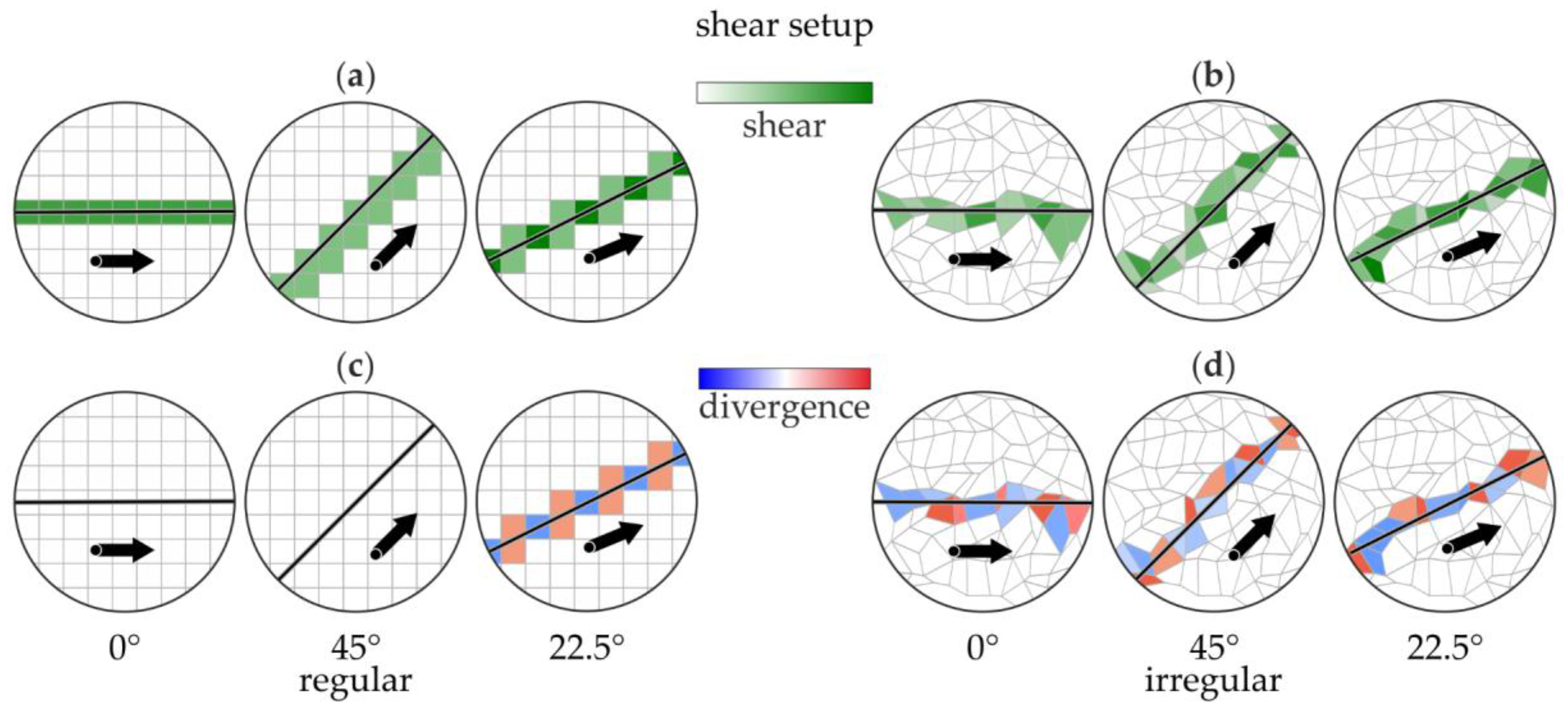
In Figure 5, one result of our numerical experiments is depicted. For this experiment, the shear setup was used. The shown parameters comprise shear deformation (Figure 5a,b) and divergence (Figure 5c,d) at three rotation angles (0°, 22.5°, and 45°). As a manifestation of the purely numerically generated BDE, we observe alternating deformation patterns at particular rotation angles. In this setup with no divergent motion, artificial openings and closings are generated. In irregular grids the occurrence of the BDE is independent from the rotation angle, whereas in regular grids the BDE in this example is only present at the 22.5° rotation angle.
Figure 6 presents a graphical overview of the numerical experiments, showing the normalized cumulative deformation rates and their dependency on the rotation angle for the three described test setups and five grid layouts. As described in Section 2.3, the BDE is reflected in the deviation of the cumulative deformation rate from the corresponding theoretical rate (first row in Figure 6) and is given per unit crack and fraction of sliding distance.
For openings and closings, for example, a BDE of, e.g., 0.2 (Q1 and 22.5°) means that there is an uncertainty of 20% of the sliding distance per unit crack. Thus, for a 100 km long crack and a sliding distance of 1 km the artificial opening (and closing) would be 20 km2, which corresponds to the case reported in Bouillon and Rampal [17]. We observe the highest BDE for the shear setup and the grid layout T1, e.g., at a rotation angle of −45°, where the mean total deformation rate per unit crack and fraction of sliding distance is 1.7. Because we obtain a theoretical total deformation rate of 1.0 for the shear setup, the BDE is 0.7 or 70% of the sliding distance per unit crack. In the irregular grids (Q2 and T3) the deviation between the normalized mean deformation rates and the corresponding theoretical values is constant over the rotation angle (see Figure 5), but is nevertheless not negligible (values Q2 and T3). In summary, all numerical experiments show that except for certain rotation angles at regular grid layouts (e.g., 0° in Q1, T1, and T2) one needs to consider the BDE. Consequently, deformation parameters are generally overestimated. In our numerical experiments only the vorticity, the divergence, and the divergence components (opening and closing) in the divergence setup behave as theoretically expected; i.e., here the BDE is zero.
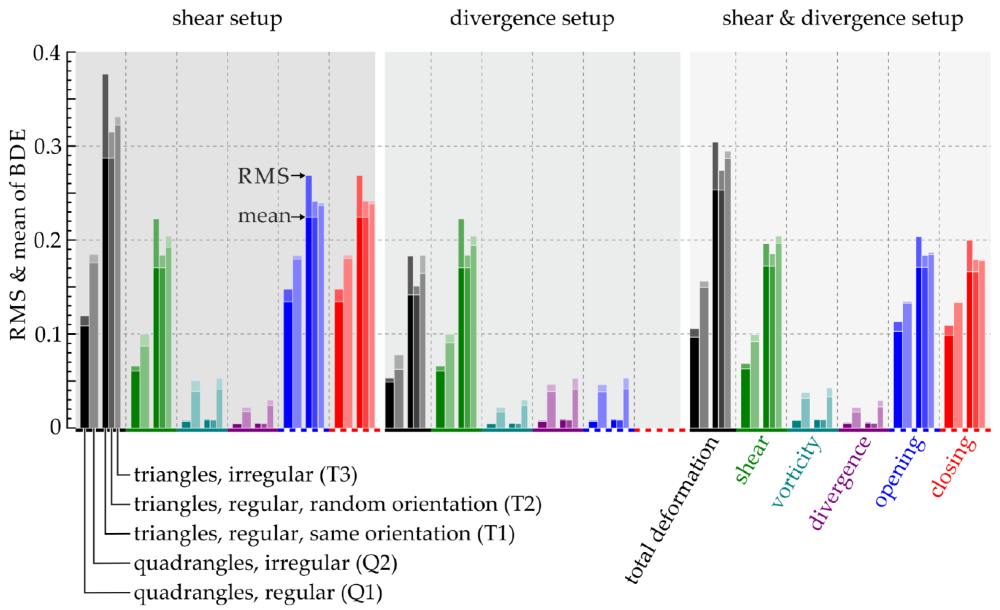
Figure 7 shows the mean absolute BDE and the root mean square BDE (Equations (17) and (18)) for the described setups and grids. We found a much higher BDE for the grids of triangles (T1, T2, and T3) than for the grids of quadrangles (Q1 and Q2), and the lowest BDE for the regular grid layout (Q1). In addition, we observe a BDE in the shear parameter of the same magnitude in all three setups. The error of the divergence components (opening and closing) is high for the shear and shear and divergence setup, but very low for pure divergence. The total divergence and the vorticity show no significant error in all three test setups.
4. Discussion
Both error types (PDRE and BDE) can have a large impact on the computed deformation parameters and their statistics. The drift detection errors that propagate into the calculations of deformation can lead to an error that can be as large as the magnitude of the deformation parameters. Thus, a high accuracy (low error level) of the drift detection algorithm is required when sea ice deformation is derived from the drift vectors. In this context, methods to improve drift detection algorithms considering discontinuities due to deformation zones are very important (e.g., [18]). A displacement error of 0.1 km, as reported in Lindsay and Stern [16], for example, reflects a comparatively high accuracy and, thus, the given PDRE of 0.005 (0.5%) per day is not generally applicable. As indicated in the introduction, adverse conditions such as low contrasts and lacking structures in the SAR intensity images which are used to retrieve the displacement may lead to unreliable results (e.g., [14]). However, up to now, a robust method to quantify the resulting tracking error has not been published.
Equations (13) and (14) mean that a short time interval and a small grid cell size increase the PDRE of the deformation parameters. However, it should be noted that the time interval corresponds to the temporal gap between the acquisitions of the SAR images and is a scaling parameter, from which the error in displacement is converted into an error of velocity. The increase of the time interval only makes sense if the trackable sea ice patterns or features are temporally stable. In addition, Equations (13) and (14) should be interpreted in terms of the ratio between a given drift retrieval error and the cell size: the PDRE is large if the drift retrieval error is large relative to the given cell dimension (see Figure 4).
The layout of the deformation grid plays a key role and affects both error types. For the PDRE, Equations (13) and (14) provide examples. The BDE depends on how well the real path of a discontinuity can be approximated in a given grid.
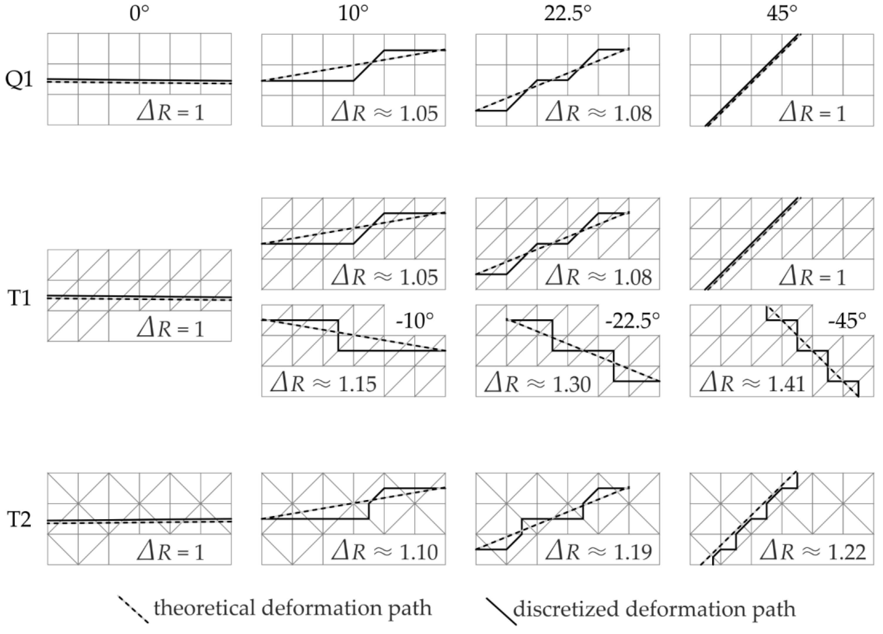
Figure 8 explains the reason for having a BDE and how it changes with the rotation angle in regular grids. Due to the discretization, the precise progression of the deformation, indicated by the dashed line, cannot be pictured. Instead, one obtains a stepped pattern (solid line). As a result, the path of the deformation feature is quantized from grid cell to grid cell, which means, e.g., that the length of the feature is larger than the real one, except in a few cases (in Figure 8 those for which solid and dashed lines are parallel). The difference in length between the theoretical and discretized path is proportional to the change in the deformation rate of the shear component in the shear setup (). In irregular grids the BDE is equally distributed over all rotation angles because the discretization results in an unsystematic change of the deformation path.
The observed lack of symmetry of the BDE magnitude in the regular triangle grid T1 (Figure 6) can also be explained considering the angle between deformation structure and grid cell boundary. As shown in Figure 8 (T1 at 45 ° and −45 °), the orientation of the triangles forming the grid affects the actual path of the discretized deformation feature and, thus, the deformation rate and the BDE crucially.
The artificial opening and closing observed in Figure 6 is also a result of the discretized path of the deformation. As shown in Figure 9 the discretization produces an artificial angle between the deformation feature and the direction of the drift vector at most rotation angles. Thus, the deformation feature and the drift vectors are not parallel and artificial openings and closings are computed, which appear as alternating patterns.
At the expense of a coarser spatial resolution it is possible to reduce the BDE (especially the artificial opening and closing). An averaging over multiple grid cells after the deformation calculation (e.g., [17]) or enlarging the deformation cell to increase the number of points on the line integral (e.g., Equation (16) in Lindsay and Stern [16]) reduce the BDE, approximately by the same magnitude. Βy using our numerical test setups and an averaging kernel of 2 × 2 grid cells or a line integral calculated using eight instead of four points, the BDE reduces in both cases by 40%–70% depending on the deformation parameter and the grid layout.
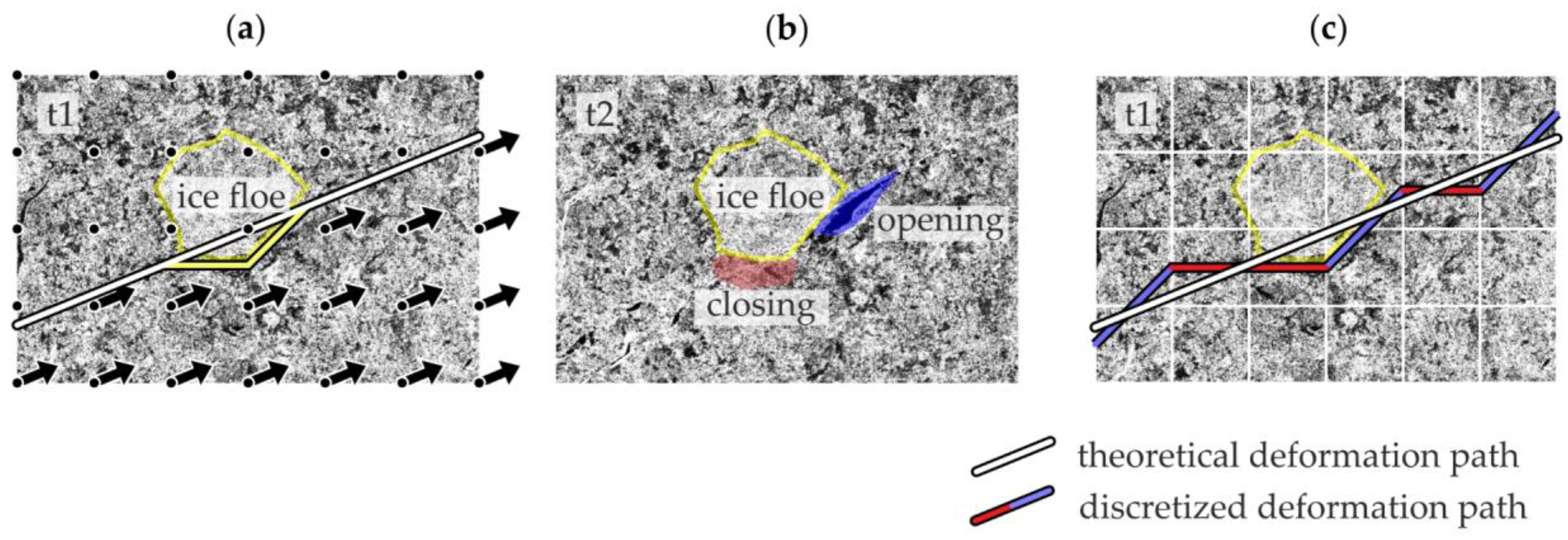
However, it should be noted that not all alternating patterns are artificially generated. Figure 10 shows that in real-world situations, the curve representing the deformation feature often has to be composed of segments of different directions. A straight shear deformation is interrupted by an ice floe, which covers only four cells of the grid (white lines visible in Figure 10c). In this example the discrete deformation path at the location of the floe is closer to reality than the theoretical path and the alternating patterns of opening and closing around the ice floe are real and need to be preserved. To our knowledge, a corresponding adaptive method has not yet been devised.
5. Conclusions
In this study we investigated how two main types of errors affect the calculation of the deformation parameters divergence, shear, vorticity, and total deformation from a field of drift (displacement) vectors. The latter are retrieved from a pair of SAR intensity images. The first error type (denoted PDRE, Propagated Drift Retrieval Error) is caused by propagation of the error in the estimation of the displacement vectors from which the drift is obtained (tracking error). This error is assumed to be random. The second type of error (Boundary Definition Error BDE) arises from discretizing a line integral on the grid of drift vectors.
For the first type we presented equations from which the standard uncertainty of the respective deformation parameter can be evaluated. We found that the PDRE can be of the same order of magnitude as the deformation parameter itself. The major problem, however, is to obtain a robust estimate of the drift retrieval error (tracking error) which may vary spatially and temporally.
For studying the BDE, we performed numerical experiments on regular and irregular grids consisting of triangles or quadrangles, and simulated pure shear, pure divergence/convergence, and a mixture of both. We showed that the BDE depends on the orientation of the deformation feature relative to the grid boundaries. Thus, the spatial invariance of the deformation parameters is not strictly valid because of discretization. The lowest BDE is obtained on square grids but they reveal a dependency on the orientation of the deformation feature relative to the grid. This is also the case for triangles, for which the error is larger than for the squares. The dependency on orientation of the deformation zone is avoided when irregular grids (triangles, quadrangles) are used. For those grids, however, the error is larger compared with regular grids. Thus, the preferential grid layout to minimize the BDE is a regular distributed grid of squares with as much drift information as possible on the cell boundary (e.g., eight points on the line integral instead of four).
The BDE depends on the orientation, length, and type of deformation. The mean BDE (over all possible orientations) per unit crack is between 0.1 and 0.3 of the sliding distance. We confirmed the error reported in Lindsay and Stern [16], which is 0.15 (15%) for the opening and closing component in a shear setup and grid of squares (see Figure 7). For a grid of triangles we get a much higher BDE (0.24) than that given by Bouillon and Rampal [17] (0.18). The reason for this is the larger range of rotation angles considered in our study.
We did not carry out a direct comparison of both error types, since they depend on different highly variable parameters which largely influence the ratio between both types. However, the presented equations and results enable the reader to estimate errors for specific cases. For studies of deformation it is important to understand that the effect of uncertainties in a sea ice drift field and the influence of the grid layout can have a large impact on the computed parameters and their statistics and must always be considered.
Acknowledgments
Jakob Griebel was funded by the Helmholtz Alliance “Remote Sensing and Earth System Dynamics”, WP-C5, which we gratefully acknowledge. We used Copernicus Sentinel-1 data and an Envisat ASAR image pair provided by ESA, Cat-1 project C1P.5024.
Author Contributions
Jakob Griebel developed and performed the numerical experiments and prepared the results for the paper. Wolfgang Dierking worked on the analytical part of error propagation and contributed to the conception of the work. Both authors wrote the text.
Conflicts of Interest
The authors declare no conflict of interest.
References
- Dierking, W. Sea Ice Monitoring by Synthetic Aperture Radar. Oceanography 2013, 26, 100–111. [Google Scholar] [CrossRef]
- Fily, M.; Rothrock, D.A. Opening and closing of sea ice leads: Digital measurements from synthetic aperture radar. J. Geophys. Res. 1990, 95. [Google Scholar] [CrossRef]
- Dierking, W.; Dall, J. Sea-Ice Deformation State From Synthetic Aperture Radar Imagery—Part I: Comparison of C- and L-Band and Different Polarization. IEEE Trans. Geosci. Remote Sens. 2007, 45, 3610–3622. [Google Scholar] [CrossRef]
- Linow, S.; Hollands, T.; Dierking, W. An assessment of the reliability of sea-ice motion and deformation retrieval using SAR images. Ann. Glaciol. 2015, 56, 229–234. [Google Scholar] [CrossRef]
- Pedersen, L.T.; Saldo, R.; Fenger-Nielsen, R. Sentinel-1 results: Sea ice operational monitoring. In Proceedings of the 2015 IEEE International Geoscience and Remote Sensing Symposium (IGARSS), Milan, Italy, 26–31 July 2015. [Google Scholar]
- Li, S.; Cheng, Z.; Weeks, W.F. A grid-based algorithm for the extraction of intermediate-scale sea-ice deformation descriptors from SAR ice motion products. Int. J. Remote Sens. 1995, 16, 3267–3286. [Google Scholar]
- Thomas, M.; Geiger, C.A.; Kambhamettu, C. High resolution (400 m) motion characterization of sea ice using ERS-1 SAR imagery. Cold Reg. Sci. Technol. 2008, 52, 207–223. [Google Scholar] [CrossRef]
- Stern, H.L.; Moritz, R.E. Sea ice kinematics and surface properties from RADARSAT synthetic aperture radar during the SHEBA drift. J. Geophys. Res. 2002, 107. [Google Scholar] [CrossRef]
- Muckenhuber, S.; Korosov, A.A.; Sandven, S. Open-source feature-tracking algorithm for sea ice drift retrieval from Sentinel-1 SAR imagery. Cryosphere 2016, 10, 913–925. [Google Scholar] [CrossRef]
- Korosov, A.; Rampal, P. A Combination of Feature Tracking and Pattern Matching with Optimal Parametrization for Sea Ice Drift Retrieval from SAR Data. Remote Sens. 2017, 9, 258. [Google Scholar] [CrossRef]
- Melling, H. Detection of features in first-year pack ice by synthetic aperture radar (SAR). Int. J. Remote Sens. 1998, 19, 1223–1249. [Google Scholar] [CrossRef]
- Vesecky, J.F.; Smith, M.P.; Samadani, R. Extraction Of Lead And Ridge Characteristics From SAR Images Of Sea Ice. IEEE Trans. Geosci. Remote Sens. 1990, 28, 740–744. [Google Scholar] [CrossRef]
- Linow, S.; Dierking, W. Object-Based Detection of Linear Kinematic Features in Sea Ice. Remote Sens. 2017, 9, 493. [Google Scholar] [CrossRef]
- Hollands, T.; Linow, S.; Dierking, W. Reliability Measures for Sea Ice Motion Retrieval From Synthetic Aperture Radar Images. IEEE J. Sel. Top. Appl. Earth Obs. Remote Sens. 2015, 8, 67–75. [Google Scholar] [CrossRef] [Green Version]
- Thorndike, A.S.; Colony, R. Sea ice motion in response to geostrophic winds. J. Geophys. Res. 1982, 87. [Google Scholar] [CrossRef]
- Lindsay, R.W.; Stern, H.L. The RADARSAT Geophysical Processor System: Quality of Sea Ice Trajectory and Deformation Estimates. J. Atmos. Ocean. Technol. 2003, 20, 1333–1347. [Google Scholar] [CrossRef]
- Bouillon, S.; Rampal, P. On producing sea ice deformation data sets from SAR-derived sea ice motion. Cryosphere 2015, 9, 663–673. [Google Scholar] [CrossRef]
- Griebel, J.; Dierking, W. Method to Improve High-Resolution Sea Ice Drift Retrievals in the Presence of Deformation Zones. Remote Sens. 2017, 9, 718. [Google Scholar] [CrossRef]
- Muckenhuber, S.; Sandven, S. Open-source sea ice drift algorithm for Sentinel-1 SAR imagery using a combination of feature tracking and pattern matching. Cryosphere 2017, 11, 1835–1850. [Google Scholar] [CrossRef]
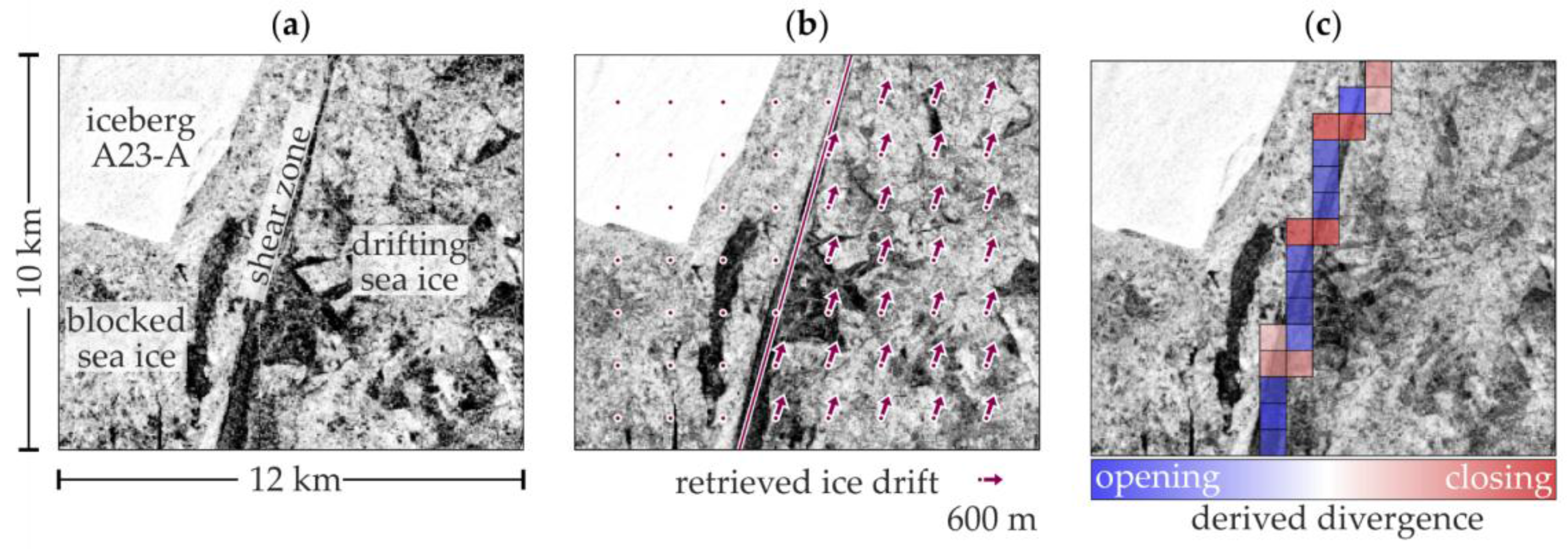
Figure 1.
Envisat ASAR (Advanced Synthetic Aperture Radar) scene acquired in the Weddell Sea showing the artificial opening and closing as a result of the boundary definition error (BDE). (a) The ice on the left side is blocked by an iceberg; hence, a shear zone is formed between stationary and drifting ice. (b) Ice drift vectors determined with a pattern matching approach described in Thomas et al. [7]. (c) Divergence calculated from the drift vectors, revealing both opening and closing of the ice (although the expected divergence is zero).

Figure 2.
Regular (a) and irregular (b) deformation grids of squares. For triangles, three different constellations used in our study are shown: regular ((c) and (d)) and irregular (e). The positions of grid vertices correspond to the origins of the drift vectors.
Figure 2.
Regular (a) and irregular (b) deformation grids of squares. For triangles, three different constellations used in our study are shown: regular ((c) and (d)) and irregular (e). The positions of grid vertices correspond to the origins of the drift vectors.
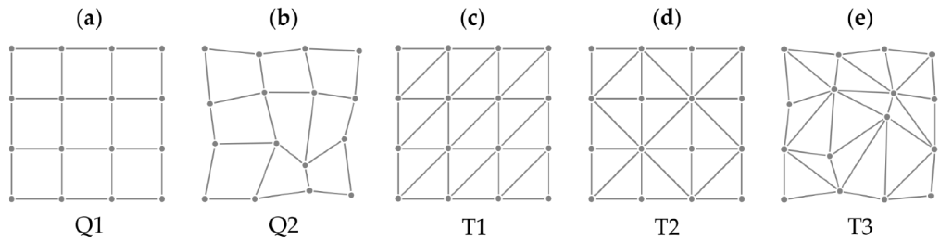
Figure 3.
Test setups for the numerical experiments. (a) Shear setup, (b) divergence setup, and (c) shear and divergence setup with the various regions separated by the deformation feature (black line). At the bottom: The two vector distributions, regular (d) and irregular (f), and examples for rotation ((e,g)). D is the length of the discontinuity segment and S is the sliding distance (relative displacement) along the corresponding discontinuity segment.

Figure 4.
Propagated drift retrieval error (PDRE) per day (in a grid consisting of squares with sides of length L) for typical time gaps between synthetic aperture radar (SAR) image pairs used for deriving sea ice drift, given a realistic range of tracking errors. The PDRE of deformation parameters derived from RGPS (RADARSAT Geophysical Processor System) data reported in Lindsay and Stern [16] is marked by a cross.
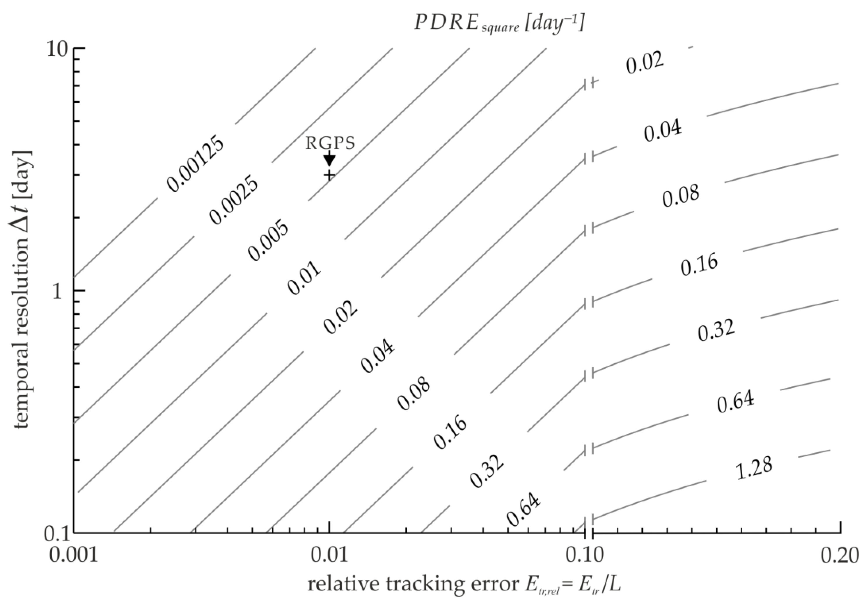
Figure 5.
Example from results of the numerical shear experiment, here at rotation angles 0°, 22.5°, and 45°. Parameters shear and divergence in a regular (a and c) and an irregular (b and d) grid, respectively. Openings are shown in blue and closings in red.
Figure 5.
Example from results of the numerical shear experiment, here at rotation angles 0°, 22.5°, and 45°. Parameters shear and divergence in a regular (a and c) and an irregular (b and d) grid, respectively. Openings are shown in blue and closings in red.

Figure 6.
Mean deformation rate per unit crack and fraction of sliding distance for parameters total deformation, shear, vorticity, and divergence (including separation between opening and closing) as a function of the rotation angle. The corresponding theoretical rates are depicted in the uppermost plots.
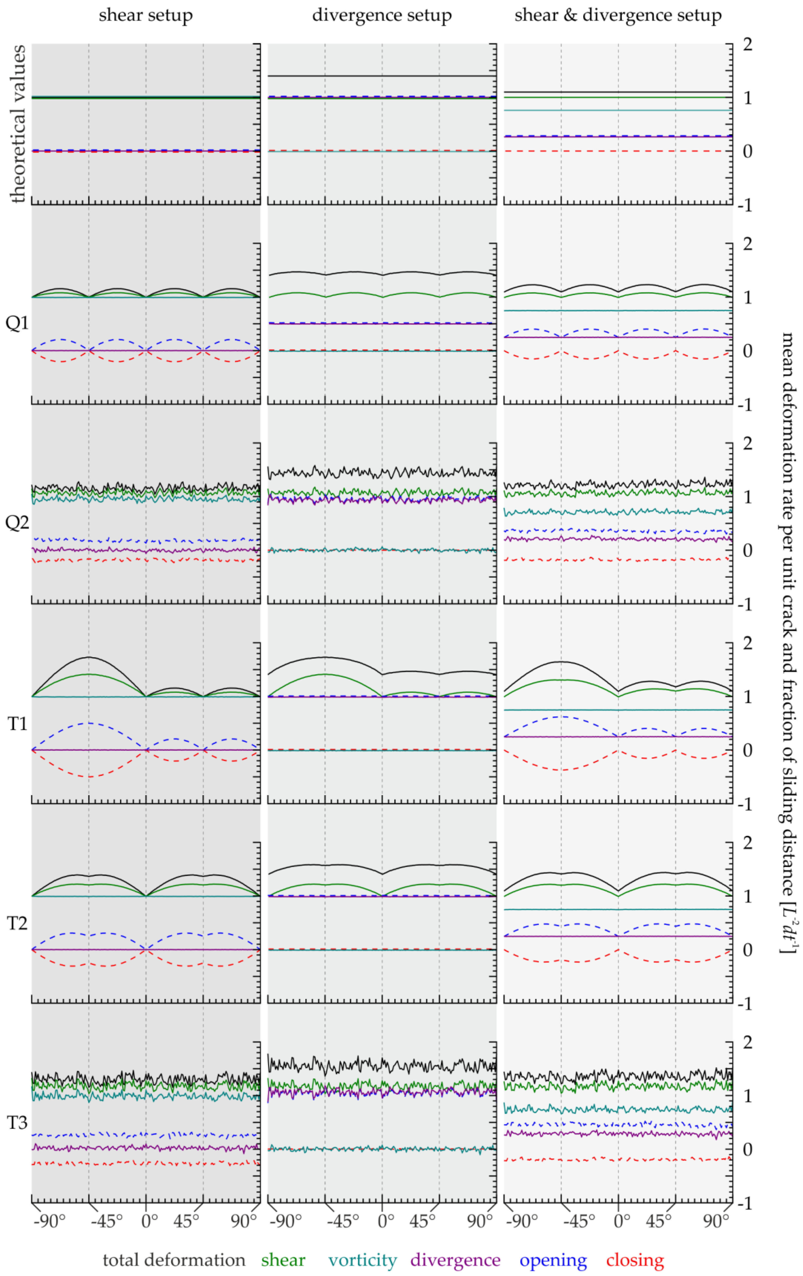
Figure 7.
The RMS and mean of BDE for all deformation parameters and grid layouts, integrated over all rotation angles (Equations (17) and (18)).
Figure 7.
The RMS and mean of BDE for all deformation parameters and grid layouts, integrated over all rotation angles (Equations (17) and (18)).

Figure 8.
Discretized (solid line) and theoretical (dashed) path of a deformation feature, here shown for two grids with different arrangements of triangles.
Figure 8.
Discretized (solid line) and theoretical (dashed) path of a deformation feature, here shown for two grids with different arrangements of triangles.

Figure 9.
Artificial patterns of opening and closing generated by the discretization of the deformation path and the resulting angle between deformation feature and drift vectors.
Figure 9.
Artificial patterns of opening and closing generated by the discretization of the deformation path and the resulting angle between deformation feature and drift vectors.
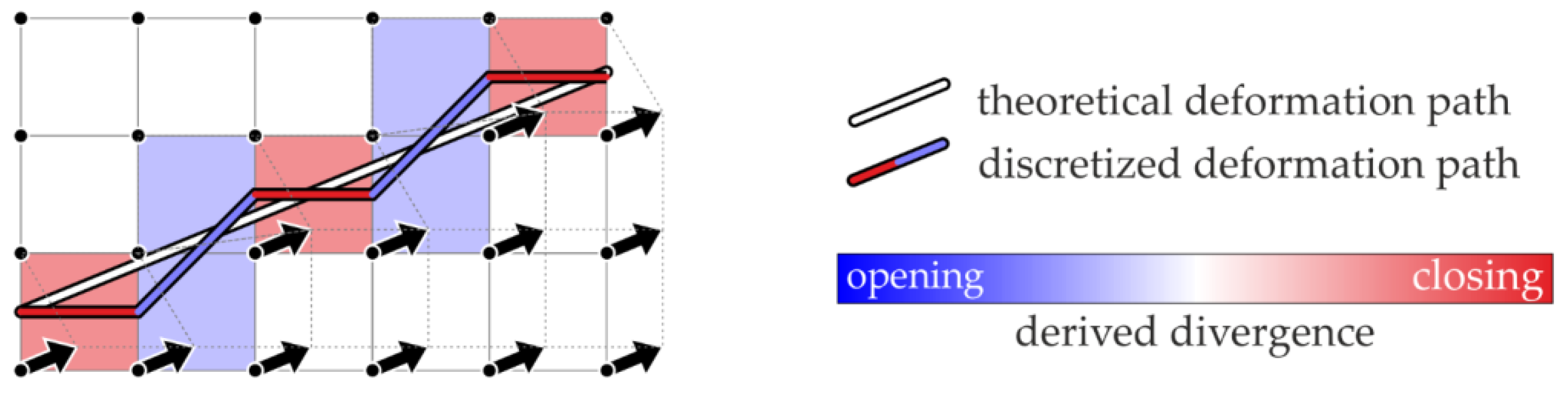
Figure 10.
Sentinel-1 image acquired over Arctic sea ice showing an example of a small ice floe locally changing the path of the discontinuity (a). The calculated opening and closing are real, which can be recognized at the margin of the ice floe (b). The discrete deformation path at the location of the floe is closer to reality than the theoretical path (c).

© 2018 by the authors. Licensee MDPI, Basel, Switzerland. This article is an open access article distributed under the terms and conditions of the Creative Commons Attribution (CC BY) license (http://creativecommons.org/licenses/by/4.0/).
Share and Cite
MDPI and ACS Style
Griebel, J.; Dierking, W. Impact of Sea Ice Drift Retrieval Errors, Discretization and Grid Type on Calculations of Ice Deformation. Remote Sens. 2018, 10, 393. https://doi.org/10.3390/rs10030393
AMA Style
Griebel J, Dierking W. Impact of Sea Ice Drift Retrieval Errors, Discretization and Grid Type on Calculations of Ice Deformation. Remote Sensing. 2018; 10(3):393. https://doi.org/10.3390/rs10030393
Chicago/Turabian StyleGriebel, Jakob, and Wolfgang Dierking. 2018. "Impact of Sea Ice Drift Retrieval Errors, Discretization and Grid Type on Calculations of Ice Deformation" Remote Sensing 10, no. 3: 393. https://doi.org/10.3390/rs10030393
Note that from the first issue of 2016, this journal uses article numbers instead of page numbers. See further details here.