Hyperspectral Classification Based on Texture Feature Enhancement and Deep Belief Networks


1
The State Key Lab. of Integrated Service Networks, School of Telecommunications Engineering, Xidian University, Xi’an 710071, China
2
The Department of Electronic and Computer Engineering, Mississippi State University, Starkville, MS 39762, USA
*
Author to whom correspondence should be addressed.
Remote Sens. 2018, 10(3), 396; https://doi.org/10.3390/rs10030396
Submission received: 2 January 2018
/
Revised: 14 February 2018
/
Accepted: 2 March 2018
/
Published: 4 March 2018
(This article belongs to the Special Issue Hyperspectral Imaging and Applications)
Abstract
:With success of Deep Belief Networks (DBNs) in computer vision, DBN has attracted great attention in hyperspectral classification. Many deep learning based algorithms have been focused on deep feature extraction for classification improvement. Multi-features, such as texture feature, are widely utilized in classification process to enhance classification accuracy greatly. In this paper, a novel hyperspectral classification framework based on an optimal DBN and a novel texture feature enhancement (TFE) is proposed. Through band grouping, sample band selection and guided filtering, the texture features of hyperspectral data are improved. After TFE, the optimal DBN is employed on the hyperspectral reconstructed data for feature extraction and classification. Experimental results demonstrate that the proposed classification framework outperforms some state-of-the-art classification algorithms, and it can achieve outstanding hyperspectral classification performance. Furthermore, our proposed TFE method can play a significant role in improving classification accuracy.

1. Introduction
Hyperspectral imagery with hundreds of narrow spectral channels provides wealthy spectral information. With very high spectral resolution, hyperspectral data has been of great interest in many practical applications, such as in agriculture, environment, surveillance, medicine [1,2,3,4] etc. Hyperspectral classification is a key technique employed in aforementioned applications. A majority of classification methods have been promoted in the last several decades to distinguish physical objects and classify each pixel into a unique land-cover label, such as maximum likelihood [5], minimum distance [6], K-nearest neighbors [7,8], random forests [9], Bayesian models [10,11], neural networks, etc., and their improvements [12,13,14,15]. Among these supervised classifiers, one of the most important classifiers is kernel-based support vector machine (SVM), which can also be considered as a kind of neural network. It can achieve superior hyperspectral classification accuracy via building an optimal hyperplane to best separate training samples.
In addition, sparse representation based on an over-complete signal dictionary has gained great attention in the literature. Sparse representation-based classification (SRC) [16,17,18] and collaborative representation classification (CRC) [19,20] are proposed from a different aspect: they do not adopt the traditional training–testing fashion. Such classification methods do not need any prior knowledge about probability density distribution of the data. To further enhance the performance of SRC and CRC, Du and Li [21] utilized a diagonal weight matrix to adaptively adjust the regularization parameter. To address the issues of Hughes phenomenon in hyperspectral classification, majority of feature extraction and selection algorithms are utilized to delete redundant features from the original data. To further improve performance of hyperspectral classification, multi-features are extracted and employed for classification. For instance, Kang et al. combined spectral and spatial features through a guided filter to process pixel-wise classification map in each class [22]. Several studies [23,24,25] focused on integrating spatial and spectral information in hyperspectral imagery. In addition, texture features are considered to assist hyperspectral classification [26], and modeling of hyperspectral image textures is significant for classification and material identification.
Recent research has highlighted deep learning with deep neural networks, which can learn high-level features hierarchically. They have demonstrated their potential in image classification, which also motivated successful applications of deep models on hyperspectral image classification. The classic deep learning method is convolutional neural networks (CNN), which plays a dominant role in visual-based issues. The local receptive fields of CNN can extract spatial-related features at high levels. Fukushima [27] introduced the motivations of CNNs. Ciresan and Lee et al. [28,29] depicted the invariants of CNNs. Chen et al. proposed 2-D CNN and 3-D CNN [30] to capture deep abstract and robust features, yielding superior hyperspectral classification performance. Although CNNs are typical supervised models, a massive training dataset is needed to trigger their powers. Unfortunately, a limited number of labeled samples are usually given in hyperspectral imagery. Deep belief networks (DBNs) [31] and stacked autoencoders (SAEs) [32] are also very promising deep learning methods for hyperspectral classification with limited training samples.
In this paper, we mainly investigate the DBN for its suitability and practicality to hyperspectral classification. A novel hyperspectral classification framework is proposed based on an optimum DBN. To acquire desirable performance, we also promote an advanced algorithm to enhance the texture features of hyperspectral imagery. The main contributions of this paper are summarized below.
- We first promote a band group method to separate the bands of hyperspectral data into different band groups. Multi-texture features are used to select a sample band in each band group.
- We propose a novel algorithm to enhance the texture features of hyperspectral data. We advocate the use of guided filter to complete the procedure of texture feature enhancement (TFE).
- An optimal DBN structure is proposed with consideration of learning and deep features extraction. The learned features are exploited in Softmax to address the classification problem. Furthermore, with enhanced texture features, accurate classification maps can be generated by considering spatial information.
The rest of the paper is organized into four sections. Section 2 is a brief description of related work. In Section 3, we detail our proposed DBN model. Datasets and parameters setting are demonstrated in Section 4. Experimental results and discussions are depicted in Section 5. Section 6 draws the conclusion of this paper.
2. The Related Work
A deep belief network (DBN) is a model that is first pre-trained in an unsupervised way, and then the available labeled training samples are used to fine-tune the pre-trained model through optimizing a cost function defined over the labels of training samples and their predictions.
The original DBN, published in Science [33], uses a generative model in the pre-training procedure, and uses back-propagation in the fine-tuning stage. This is very useful when the number of training samples is limited, such as in the case of hyperspectral remote sensing. DBN can be efficiently trained in an unsupervised, layer-by-layer manner where the layers are typically made of restricted Boltzmann machines (RBM). Thus, to explain the structure and theory of the DBN, we first describe its main component, the RBM.
2.1. Restricted Boltzmann Machines (RBM)
An RBM generally uses unsupervised learning, which can be interpreted as stochastic neural networks. It was originally developed to form a distributed representation. It is a two layer-wise network, which is composed of visible and hidden units. Learning RBM only allows the full connection between visible and hidden units, and does not allow connection between two visible units or connections between two hidden units. With the given visible units, hidden units can be obtained via mapping of visible units. The activations of each neuron in hidden layers are independent. Meanwhile, with the given hidden units, visible units have the same effects. A typical RBM structure is depicted in Figure 1.
The visible units can be represented as , and the hidden units can be expressed as . The RBM model is a kind of energy-based models in which the joint distribution of the layers can be expressed as Boltzmann distribution. Energy-based probabilistic models define a probability distribution through an energy function as:
where the normalization constant is called the partition function by analogy with physical systems:
A joint configuration of the units has an energy given by:
where ; represents the weight connecting the visible unit i and the hidden unit j; and denote the bias terms of visible and hidden layers, respectively; n and m are the total visible and hidden unit numbers; and and represent the states of visible unit i and hidden unit j.
Due to the specific structure of RBMs, visible and hidden units are conditionally independent, as given by:
where is the logistic function defined as
Overall, an RBM has five parameters: , , , and , where , and are achieved via learning, is input, and is output. , and can be learned and updated via the contrastive divergence (CD) method as
where denotes the learning rate, represents the reconstructed probability distribution, and and are the reconstruction of visible and hidden unit, respectively. Once the states of hidden units are chosen, the visible units can be reconstructed via the hidden units sampled via Gibbs method. Then, the states of hidden units are updated through the visible units, so that the hidden units demonstrate the features of reconstruction. The distribution of visible units approximates the distribution of the real data. The learning ability of an RBM depends on whether the hidden units contain enough information of the input data.
2.2. Deep Belief Learning
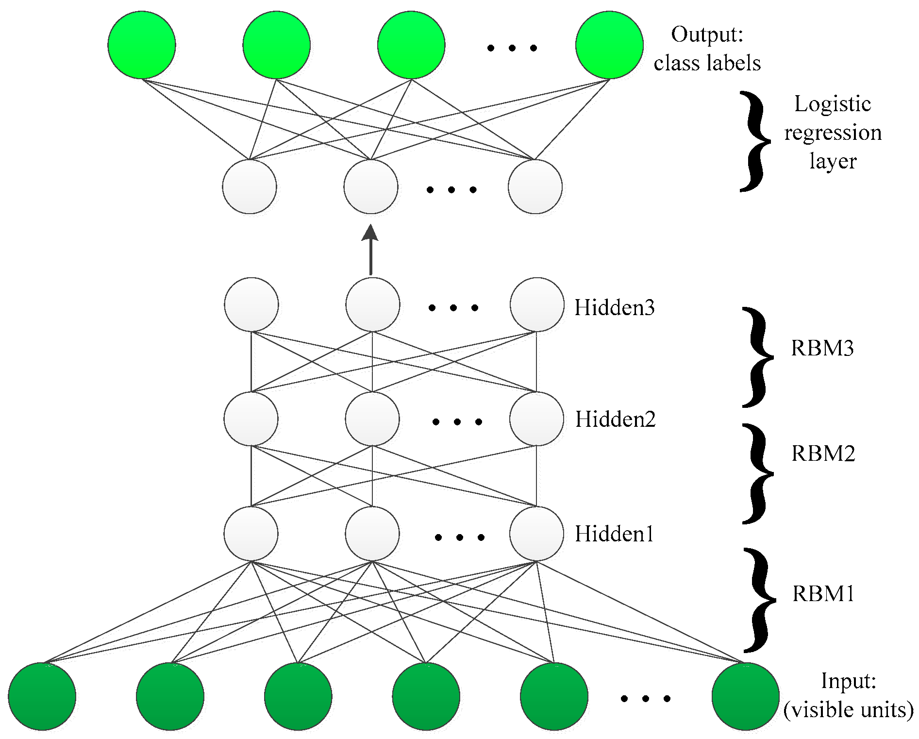
The learning ability of a single hidden layer is limited. To capture the comprehensive information of data, the hidden units of the RBM can be feed as the input (visible units) of another RBM. This kind of layer-by-layer learning structure trained in a greedy manner forms so-called Deep Belief Networks. In this way, DBN can extract deep features of image data. The structure of three-layer DBN is depicted in Figure 2.
The process of training of DBN consists of two parts: pre-training and fine-tuning. The pre-training is an unsupervised training stage that initializes the model in such a way to enhance the efficiency of supervised training. The fine-tuning process can be realized as supervised training stage, which adjusts the classifier’s prediction to match the ground truth of the data.
3. The Proposed Framework
To extract more powerful and invariant features, we propose a novel DBN hyperspectral classification algorithm based on TFE. DBN is composed of several layers of latent factors, which can be deemed as neurons of neural networks. However, the limited training samples in the real hyperspectral image classification task usually lead to many “dead” (never responding) or “potential over-tolerant” (always responding) latent factors (neurons) in the trained DBN. Our proposed framework mainly consists of three steps: band grouping and sample band selection, TFE, and DBN-based classification.
3.1. Band Grouping and Sample Band Selection
Compared to multispectral imagery, hyperspectral imagery with hundreds of spectral bands has relatively narrow bandwidths. The correlation between spectral bands needs to be considered. In our framework, we calculated all the pair wise correlation coefficient of bands, and then utilized the correlations between adjacent bands. The spectral correlation coefficients in different datasets are depicted in Figure 3.
We can obtain the correlation coefficient between adjacent bands as:
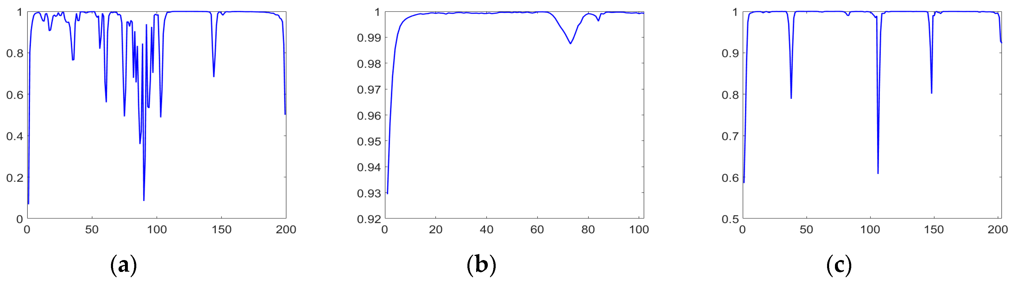
where cov is covariance and var means variance. and represent the -th and -th band channels, respectively. . Here, L denotes the number of bands of the hyperspectral dataset. Based on Equation (9), the correlation coefficients between adjacent bands in different datasets are calculated, as shown in Figure 4. We can see that the highest correlation coefficient in Indian Pines is 0.9997, and the lowest correlation coefficient is 0.0686. The spectral bands of university of Pavia have strong correlations overall, where the highest correlation coefficient is 0.9998, and the lowest correlation coefficient is 0.9294. The highest correlation coefficient in Salinas is 0.9999, and the lowest correlation coefficient is 0.5856.
Here, we design an algorithm for grouping bands rationally.
Firstly, calculate the average correlation coefficients of the adjacent bands, denoted as , which is utilized as the threshold in the following steps. It can be calculated through:
where . If the correlation coefficients of adjacent bands are greater than , these two bands are considered to have strong correlation.
Second, search local minimum values from the correlation coefficients between the adjacent bands, denoted as , where . All the elements in are compared with . If the inequality is satisfied, it indicates that the correlation between the -th band and the -th band is lower than the average correlation value, and the correlation between these two bands is considered to be weak. Then, the corresponding index group {i, j} is recorded and added to the set .
Third, band grouping depends on the stored index pairs in . For instance, with regard to index pair {i, j}, the i-th band is set as the end band of the former band group and the j-th band is set as the first band of the next band group. Thus, based on the aforementioned rules, all the bands are divided into different band groups .
After dividing all the bands of hyperspectral dataset into different band groups, a sample band with the strongest and clearest texture features is searched and selected from each group.
To extract texture features, the gray level co-occurrence matrix (GLCM) has been employed successfully. GLCM [34] is defined as a matrix of frequencies which can extract second order statistics from a hyperspectral image. The distribution in the matrix depends on the angular and distance relationship between pixels. After the GLCM is created, it can be used to compute various features. We choose the five most commonly used features in Table 1 to select a sample band from each band group. The texture feature score of each band can be calculated by Equation (11):
The sample band in each band group can be selected through:
where represents the -th band group of the dataset, , is the number of bands in the -th band group, and represent the -th band in the -th band group. Finally, the sample band set are comprised of .
3.2. Texture Feature Enhancement
As an effective edge-preserving filter, guided filter (GF) was proposed by He in 2012. It can enhance the detail of an image. Texture feature is a kind of important spatial characteristics and also has long history in image processing. In this paper, we utilize the GF in each band group to enhance the texture features of the image.
The general guided image filtering was designed for gray-scale images or color images. It is very easy to extend to multi-channel image. Firstly, the guidance image in our proposed framework is multi-channel image, denoted as , which is comprised of the copies of the band with the strongest texture features in each band group. We assume is a linear transform of in a window centered at the pixel k, and the multi-channel guided filter model can be expressed as
where is a vector, and is the channel number of the input image, is a coefficient vector, and and are scalars. The guided filter for multi-channel guidance image becomes
where is the covariance matrix of in , is an identity matrix, denotes a filtering input image which is given beforehand according to the application, is the mean of in , is the mean of in , and represents the number of pixels in .
Then, the extending guided image filtering for multi-channel images will be applied to each band group. For instance, each channel of the guidance image in Equation (14) for the -th band group is the copy of the sample band selected previously.
After guided filtering for all groups is completed, the output bands are restored to a hyperspectral image cube according to the band number. Finally, the reconstructed image data with enhanced texture features are obtained through the aforementioned steps. Figure 5 demonstrates the procedure of band grouping and TFE. We can see that, after sample bands with strongest textures are obtained, the reconstructed image data with enhanced texture feature can be achieved through the GF process.
3.3. DBN Classification Model
In this section, a DBN-based framework for hyperspectral classification with feature enhanced data is developed.
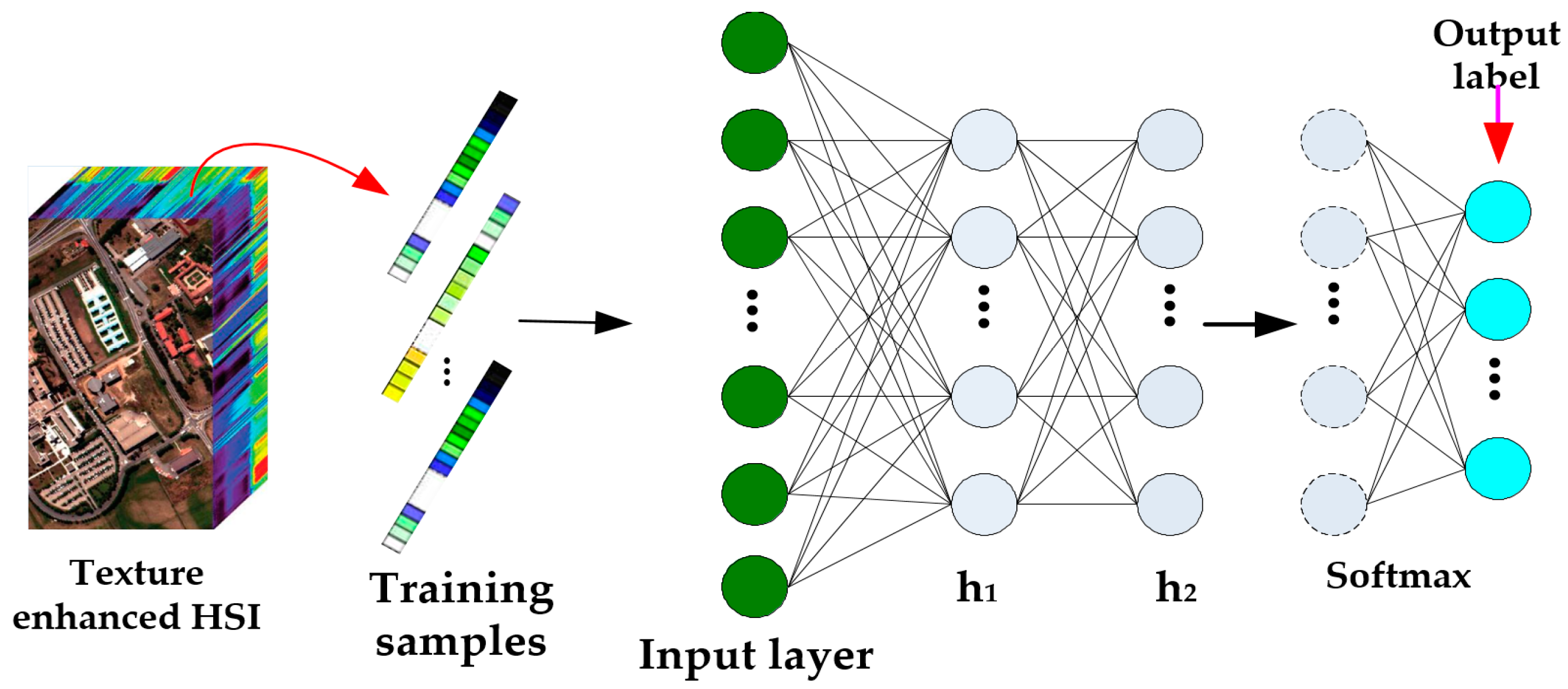
Spectral information is the most significant and direct feature, and can be directly utilized for classification. Architectures of existing methods, such as SVM and KNN, can extract spectral features but not deep enough. Therefore, only a deep architecture can make full use of the texture enhanced hyperspectral image characteristics. However, as the training samples are limited, the overfitting problem often occurs if the network is too deep, so we advocate a novel DBN framework, which has only two hidden layers (Figure 6).
The input data consist of training samples that are one-dimensional (1-D) vectors, and each pixel of a training sample is collected from the texture enhanced HSI data. For ease of description, the first hidden layer is denoted as and the second . The first layer is learned for extracting features from the input data, and the learned features are preserved in . Then, to pursue refined and abstract features, using the features contained in as the visible data of the second layer, keeps the refined features. This procedure is generally called recursive greedy learning for pre-training a DBN.
In practice, learning each layer is often performed through the -step CD, and the weights are updated using Equations (6)–(8).
To fine-tune the DBN and accomplish classification, a Softmax layer is added to the end of the network.
Now, let be a set of training samples and be the corresponding labels, where is the spectral signature of the -th sample with bands. Utilizing the maximum likelihood method, the objective function can be written as
where is the number of training samples, means the distribution of when given with the parameters of the Softmax layer, and denotes the output of the Softmax layer of the -th training sample, that is
where is the number of the hidden layers, which is set to 2 in our proposed framework, and is the number of the classes. and are the parameter vectors for the -th and -th unit of the softmax layer, respectively. is the output of the -th hidden layer, which is calculated via the input data, the weights and bias from the first layer to the -th hidden layer. To optimize the objective function, the stochastic gradient descent (SGD) algorithm is used. Finally, the label of each testing pixel is determined via the weights and biases from aforementioned steps.
4. Experiments
4.1. Datasets
In this section, three typical hyperspectral datasets, namely Indian Pines, University of Pavia and Salinas, are employed to compare the proposed DBN classification method with other state-of-the-art methods. In these experiments, we randomly select 300 labeled pixels per class for training, of which 20 samples are utilized for validation. The remaining pixels of labeled data are used for testing. Furthermore, each pixel is uniformly scaled to the range of −1 to 1.
The first experiment is Indian Pines dataset, which was gathered by Airborne Visible/Infrared Imaging Spectrometer (AVIRIS) sensor in northwestern Indiana. There are 220 spectral channels in 0.4 to 2.45 μm region with spatial resolution of 20 m. It consists of 145 × 145 pixels with 200 bands after removing 20 noisy and water absorption bands. Here, we employ 8 large classes in this experiment. The numbers of training and testing samples are listed in Table 2.
The second dataset with 610 × 340 pixels is the University of Pavia, which was acquired by the Reflective Optics System Imaging Spectrometer (ROSIS) during a flight campaign over Pavia, northern Italy. The ROSIS sensor cover 115 spectral bands from 0.43 to 0.86 μm and the geometric resolution is 1.3 m. Each pixel has 103 bands after discarding bad bands. There are 9 ground-truth classes with the number of labeled samples shown in Table 3.
The third experiment is on Salinas dataset, which was also collected by the AVIRIS sensor, capturing an area over Salinas Valley, California, with a spatial resolution of 3.7 m. The area comprises 512 × 217 pixels with 204 bands after removing noisy and water absorption bands. It mainly contains vegetables, bare soils, and vineyard fields. There are 16 different ground-truth classes, and the numbers of training and testing samples are listed in Table 4.
Our experiments are implemented using Matlab 2015b which is manufactured by Mathworks in Massachusetts, US. The CPU we employed is Intel Core i5-3470. The basic frequency is 3.200 GHz. The operation system is Win7 with 64 bits.
4.2. Parameters Tuning and Analysis
In our proposed framework, we have several parameters that need to be adjusted: the number of hidden units, the learning rate, the max epoch and the number of hidden layers. In this section, some tuning experimental results are listed for selecting proper values. Both the number of hidden layers and the number of hidden units in hidden layers play an important role in classification performance. A suitable number of hidden layers and neurons can make full use of texture enhanced hyperspectral data without over-training, and can support a fitting mapping from original hyperspectral data to hyperspectral features. In the training process of DBN, the learning rate controls the pace of learning. It implies that a too large learning rate will lead an unstable output of training, and a too small learning rate will lead a longer training process. Therefore, an appropriate learning rate can expedite our training procedure with satisfactory performance.
In Figure 7, we can see that our proposed framework achieves best classification accuracy with 200 hidden neurons in each hidden layer. It demonstrates that 200 is a suitable number of hidden neurons. Figure 8 depicts the relationship between accuracies and the learning rates. It can be seen that the values of learning rate from 0.15 to 0.2 can obtain better performance. Therefore, we select 0.15 for the first RBM, and 0.2 for the second RBM. To determine the max epoch, we set the range of max epoch from 50 to 500. Figure 9 demonstrates that, when max epoch reaches 300, our proposed framework can achieve best classification performance. Consequently, the max epoch is set to 300. Table 5 lists the accuracies achieved with different numbers of hidden layers in DBN. When employing two hidden layers, the classification performance of DBN can achieve superior results. Thus, in our proposed framework, we set the number of hidden layers to 2.
In our paper, we utilize Graycomatrix function in Matlab to calculate the GLCM. The parameters used in experiments are “NumLevels” and “Offset”, and they are set to 8 and [0, 3; −3, 3; −3, 0; −3, −3], respectively.
4.3. Evaluation Criteria
The evaluation criteria used in our paper are overall accuracy (OA), average accuracy (AA), precision, and Kappa. Especially, OA, Precision and Kappa are highlighted for assessment of the proposed framework.
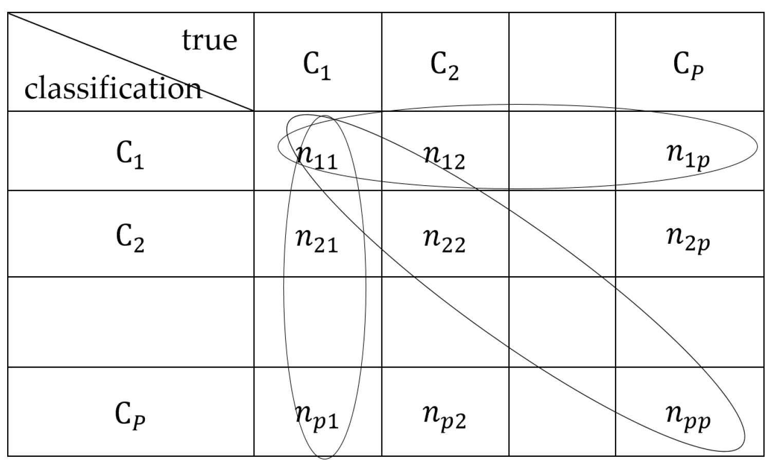
Figure 10 demonstrates a p-class confusion matrix. Based on Figure 10, AA and precision can be derived as [35]
where p is the number of classes. N is the total number of the hyperspctral image data samples and . nii is the number of hyperspectral image samples in the i-th class to be classified into the i-th class, and nji is the number of hyperspectral image samples in the i-th class to be classified into the j-th class.
We also take the nonparametric McNemar’s test based on the standardized normal test statistic to evaluate the statistical significance in the improvement of OA with different hyperspectral classification algorithms. The McNemar’s test statistic for two different algorithms noted as Algorithm 1 and Algorithm 2 can be calculated as [36]:
where denotes the number of samples misclassified using Algorithm 2 but not Algorithm 1, and means the number of samples misclassified using Algorithm 1 but not Algorithm 2. is the absolute value of . For 5% level of significance, the value is 1.96. If a value is greater than this quantity, the two classification algorithms have significant discrepancy.
5. Experimental Results and Discussion
In this section, the proposed TFE and the novel classification framework will be evaluated and the relevant results will be summarized and discussed in detail.
5.1. Compared Methods and Band Groups
To analyze and evaluate our proposed algorithm, which combines the TFE and the optimal DBN efficiently, existing algorithm, such as SVM with Radial Basis Function kernel (SVM-RBF), the Radical Basis Function neural network (RBFNN) and CNN, are employed for comparison purpose. Besides, we also compare with a state-of-the-art spectral–spatial algorithm called EPF-G-c [22]. All these algorithms are widely used with excellent performance in hyperspectral image classification tasks, especially EPF-G-c. In addition, for evaluating our proposed texture feature enhancement (TFE) algorithm, we also applied TFE algorithm on the traditional SVM-RBF and RBFNN. All experiments are repeated 10 times with the average classification results demonstrated for comparison.
According to our proposed band grouping solution, the bands of Indian Pines can be divided into 41 groups: 1, 2, 3, 4–17, 18, 19–33, 34, 35, 36, 37–56, 57, 58–60, 61, 62, 63–74, 75, 76, 77–82, 83, 84, 85, 86, 87, 88, 89, 90, 91, 92–93, 94, 95, 96–97, 98–102, 103, 104, 105, 106–143, 144, 145, 146–198, 199 and 200. The bands of University of Pavia can be divided into 19 groups: 1, 2, 3, 4, 5, 6, 7, 8–68, 69, 70, 71, 72, 73, 74, 75, 76, 77, 78–84 and 85–103. The bands of Salinas can be divided into 21 groups: 1, 2, 3, 4, 5–35, 36, 37, 38, 39, 40, 41–104, 105–106, 107, 108, 109–146, 147, 148, 149–201, 202, 203 and 204. All these band groups are employed in the TFE algorithm.
5.2. Discussion on Effectiveness of the Proposed TFE
Figure 11 demonstrates the reconstructions of border and inner pixels of four classes after TFE in Indian Pines dataset. The first image of each row depicts the locations of border and inner pixels. The reconstruction and reconstructed error of the border pixel are demonstrated in the second image of each row. Meanwhile, the reconstruction and reconstructed error of the inner pixel are demonstrated in the third image.
In hyperspectral classification, some spectra of the hyperspectral image are distorted through imaging noise or low spatial resolution, especially border-pixels, therefore the difficulty of hyperspectral classification primarily focuses on the correct classification of the border pixels. In Figure 11, it can be seen that, by utilizing TFE, the reconstructed border pixels become different from the original border pixels, and the reconstructed inner pixels are nearly the same as the original inner pixels, which implies that TFE plays an important role for border pixels. TFE can make border pixels distinct with its characteristics and more similar to their original spectra. Hence, the texture feature of the hyperspectral image become more obvious and clear. Consequently, the pixels that are difficult to distinguish can be recognized more easily than before with clearer texture feature. In other words, TFE has a positive effect for enhancing hyperspectral classification performance.
5.3. Discussion on Classification Results and Statistical Test
Table 6 provides the classification performance on Indian Pines achieved by different classification algorithms: SVM, RBFNN, optimal DBN (O_DBN), SVM combined with TFE (SVM_TFE), RBFNN combined with TFE (RBFNN_TFE), CNN, EFP-G-c and our proposed framework. O_DBN denotes the optimal DBN we proposed but without TFE. The SVM_TFE and RBFNN_TFE are two algorithms combined with the TFE method. The classification accuracy of each class is also listed in this table. In Table 6, we can see that our proposed framework can obtain the superior performance compared with other algorithms. Meanwhile, the optimal DBN has the best classification accuracy compared to the other algorithms without TFE, such as SVM and RBFNN. Although EFP-G-c is an outstanding spectral–spatial hyperspectral classification algorithm, our proposed framework utilizing TFE still has slightly better classification accuracy. Besides, SVM_TFE and RBFNN_TFE outperform SVM and RBFNN, respectively. The OA of SVM_TFE is 5.06% greater than SVM, and the OA of RBFNN_TFE is 8.97% higher than RBFNN. Compared with O_DBN, the OA obtained via our proposed framework improved by 8.08% and the Kappa increased by 9.98%. All these facts indicate the successful effects of TFE and demonstrates that our proposed framework and TFE have good influence on Indian Pines in hyperspectral classification.
Table 7 lists the classification precision achieved via these different classification algorithms. In Table 7, we can see that the precision of our proposed algorithm outperforms SVM, RBFNN, O_DBN, SVM_TFE, RBFNN_TEF, CNN and EPF-G-c. In addition, the methods associated with TFE have better classification precision than without TFE.
Table 8 and Table 10 present the classification accuracy acquired via different algorithms for University of Pavia and Salinas datasets. Meanwhile, Table 9 and Table 11 also list the precisions obtained through our proposed model and other classification algorithms on different datasets. It is obvious in Table 8 and Table 10 that our proposed framework has better performance than other classification methods. Especially, we can see that all algorithms that integrate TFE outperform those without TFE. By employing the TFE, the performance of SVM increased by 5.78% in University of Pavia and 1.75% in Salinas, while the performance of RBFNN improved by 6.8% in University of Pavia and 1.55% in Salinas. The OA achieved by the proposed framework is 6.55% higher than the OA achieved via optimal DBN in University of Pavia and 3.94% larger than the OA achieved via optimal DBN in Salinas. Furthermore, the proposed classification framework has better performance than CNN and EPF-G-c. As for kappa coefficients, we can see that our proposed framework has better consistency. The possible reason is the ability of our proposed framework, as a deep network, to extract high-level features of data is stronger than the RBFN and the SVM, as shallow networks, thus the description ability of our proposed framework is more stable. In Table 9 and Table 11, the precisions obtained through our proposed model on different datasets are better than precisions achieved via other algorithms. Furthermore, our proposed TFE has a positive effect on classification accuracy.
Figure 12, Figure 13 and Figure 14 demonstrate the classification maps obtained in Indian Pines, University of Pavia and Salinas, respectively. Clearly, the classification maps shown in Figure 12, Figure 13 and Figure 14 achieved by our proposed framework are the smoothest and clearest. The classification accuracy of border pixels in these datasets is improved greatly and the boundaries of different classes are more distinct. Compared to other classification algorithms, the results of our proposed framework are better because they contain less salt-and-pepper noise.
Table 12 presents the average values achieved from Indian Pines, Pavia University and Salinas of the proposed classification framework as well as other classification algorithms. A “yes” here denotes the two classification algorithms in McNemar’s test have significant performance discrepancy. Obviously, the proposed classification framework is statistically different from its counterparts with 5% significance level.
6. Conclusions
In this paper, we investigate a novel hyperspectral classification framework based on an optimal DBN algorithm. In our proposed framework, we develop a new TFE algorithm that employs multi-texture features and band grouping method. The resulting classification framework can offer better classification accuracy than other classic algorithms. To further test our proposed TFE algorithm, a series of experiments based on the combination of the state-of-the-art algorithms and the TFE algorithm are applied on the three classic hyperspectral datasets. Experimental results demonstrate that the algorithms with TFE outperform those without TFE, which implies that our proposed TFE can play an important role in improving hyperspectral classification performance. We believe that the proposed hyperspectral classification framework based on the optimal DBN and TFE is more suitable to process hyperspectral data in practical applications when training samples are limited.
Acknowledgments
This work was partially supported by the National Nature Science Foundation of China (Nos. 61571345, 91538101, 61501346, 61502367 and 61701360) and the 111 project (B08038). It was also partially supported by the Fundamental Research Funds for the Central Universities JB170109, the Natural Science Basic Research Plan in Shaanxi Province of China (No. 2016JQ6023) and General Financial Grant from the China Postdoctoral Science Foundation (No. 2017M623124).
Author Contributions
L.J. and L.Y.S. conceived and designed the study; L.J. performed the experiments; X.B. analyzed the data; L.J. and X.B. wrote the paper; and W.K.Y. and D.Q. reviewed and edited the manuscript. All authors read and approved the manuscript.
Conflicts of Interest
The authors declare no conflict of interest. The funding sponsors had no role in the design of the study; in the collection, analyses, or interpretation of data; in the writing of the manuscript, and in the decision to publish the results.
References
- Adão, T.; Hruška, J.; Pádua, L.; Bessa, J.; Peres, E.; Morais, R.; Sousa, J.J. Hyperspectral Imaging: A Review on UAV-Based Sensors, Data Processing and Applications for Agriculture and Forestry. Remote Sens. Agric. Veg. 2017, 9, 1110. [Google Scholar] [CrossRef]
- Yokoya, N.; Chan, J.C.W.; Segl, K. Potential of Resolution-Enhanced Hyperspectral Data for Mineral Mapping Using Simulated EnMAP and Sentinel-2 Images. Remote Sens. 2016, 8, 172. [Google Scholar] [CrossRef]
- Merentitis, A.; Debes, C.; Heremans, R. Ensemble Learning in Hyperspectral Image Classification: Toward Selecting a Favorable Bias-Variance Tradeoff. IEEE J. STARS 2014, 7, 1089–1102. [Google Scholar] [CrossRef]
- He, J.; He, Y.; Zhang, C. Determination and Visualization of Peimine and Peiminine Content in Fritillaria thunbergii Bulbi Treated by Sulfur Fumigation Using Hyperspectral Imaging with Chemometrics. Molecules 2017, 22, 1402. [Google Scholar] [CrossRef] [PubMed]
- Richards, J.A.; Jia, X. Using Suitable Neighbors to Augment the Training Set in Hyperspectral Maximum Likelihood Classification. IEEE Geosci. Remote Sens. Lett. 2008, 5, 774–777. [Google Scholar] [CrossRef]
- Leonenko, G.; Los, S.O.; North, P.R.J. Statistical Distances and Their Applications to Biophysical Parameter Estimation: Information Measures, M-Estimates, and Minimum Contrast Methods. Remote Sens. 2013, 5, 1355–1388. [Google Scholar] [CrossRef]
- Zhang, J.; Mani, I. KNN Approach to Unbalanced Data Distributions: A Case Study Involving Information Extraction. In Proceedings of the ICML 2003 Learning Imbalanced Datasets, Washington, DC, USA, 21–24 August 2003. [Google Scholar]
- Mathew, J.; Luo, M.; Pang, C.K.; Chan, H.L. Kernel-based SMOTE for SVM classification of imbalanced datasets. In Proceedings of the IECON 2015 41st Annual Conference of the IEEE Industrial Electronics Society, Yokohama, Japan, 9–12 November 2015; pp. 001127–001132. [Google Scholar]
- Immitzer, M.; Atzberger, C.; Koukal, T. Tree Species Classification with Random Forest Using Very High Spatial Resolution 8-Band WorldView-2 Satellite Data. Remote Sens. 2012, 4, 2661–2693. [Google Scholar] [CrossRef]
- Dobigeon, N.; Tourneret, J.Y.; Chang, C.I. Semi-Supervised Linear Spectral Unmixing Using a Hierarchical Bayesian Model for Hyperspectral Imagery. IEEE Trans. Signal Process. 2008, 56, 2684–2695. [Google Scholar] [CrossRef] [Green Version]
- Zhang, L.; Wei, W.; Zhang, Y.; Li, F.; Yan, H. Structured sparse BAYESIAN hyperspectral compressive sensing using spectral unmixing. In Proceedings of the 2014 6th Workshop on Hyperspectral Image and Signal Processing: Evolution in Remote Sensing (WHISPERS), Lausanne, Switzerland, 24–27 June 2014. [Google Scholar]
- Yu, H.; Gao, L.; Li, J.; Li, S.S.; Zhang, B.; Benediktsson, J.A. Spectral-Spatial Hyperspectral Image Classification Using Subspace-Based Support Vector Machines and Adaptive Markov Random Fields. Remote Sens. 2016, 8, 355. [Google Scholar] [CrossRef]
- Chen, H.M.; Wang, H.C.; Chai, J.W.; Chen, C.C.C.; Xue, B.; Wang, L.; Yu, C.; Wang, Y.; Song, M.; Chang, C.I. A Hyperspectral Imaging Approach to White Matter Hyperintensities Detection in Brain Magnetic Resonance Images. Remote Sens. 2017, 9, 1174. [Google Scholar] [CrossRef]
- Kayabol, K. Bayesian Gaussian mixture model for spatial-spectral classification of hyperspectral images. In Proceedings of the 2015 23rd European Signal Processing Conference (EUSIPCO), Nice, France, 31 August–4 September 2015; pp. 1805–1809. [Google Scholar]
- Ramo, R.; Chuvieco, E. Developing a Random Forest Algorithm for MODIS Global Burned Area Classification. Remote Sens. 2017, 9, 1193. [Google Scholar] [CrossRef]
- Starck, J.; Elad, M.; Donoho, D. Image decomposition via the combination of sparse representation and a variational approach. IEEE Trans. Image Process. 2005, 14, 1570–1582. [Google Scholar] [CrossRef] [PubMed]
- Wright, J.; Yang, A.Y.; Ganesh, A.; Sastry, S.S.; Ma, Y. Robust face recognition via sparse representation. IEEE Trans. Pattern Anal. Mach. Intell. 2009, 31, 210–226. [Google Scholar] [CrossRef] [PubMed]
- Zhang, L.; Zhou, W.D.; Chang, P.C.; Yan, Z.; Wang, T.; Li, F.Z. Kernel Sparse Representation-Based Classifier. IEEE Trans. Signal Process. 2012, 60, 1684–1695. [Google Scholar] [CrossRef]
- Chen, Y.; Nasrabadi, N.M.; Tran, T.D. Hyperspectral image classification using dictionary-based sparse representation. IEEE Trans. Geosci. Remote Sens. 2011, 49, 3973–3985. [Google Scholar] [CrossRef]
- Chen, Y.; Nasrabadi, N.M.; Tran, T.D. Hyperspectral image classification via kernel sparse representation. IEEE Trans. Geosci. Remote Sens. 2013, 51, 217–231. [Google Scholar] [CrossRef]
- Li, W.; Tramel, E.W.; Prasad, S.; Fowler, J.E. Nearest regularized subspace for hyperspectral classification. IEEE Trans. Geosci. Remote Sens. 2014, 52, 477–489. [Google Scholar] [CrossRef]
- Kang, X.; Li, S.; Benediktsson, J.A. Spectral–Spatial Hyperspectral Image Classification with Edge-Preserving Filtering. IEEE Trans. Geosci. Remote Sens. 2014, 52, 2666–2677. [Google Scholar] [CrossRef]
- Chen, C.; Li, W.; Su, H.; Liu, K. Spectral-Spatial Classification of Hyperspectral Image Based on Kernel Extreme Learning Machine. Remote Sens. 2014, 6, 5795–5814. [Google Scholar] [CrossRef]
- Wang, T.; Zhang, H.; Lin, H.; Fang, C. Textural–Spectral Feature-Based Species Classification of Mangroves in Mai Po Nature Reserve from Worldview-3 Imagery. Remote Sens. 2016, 8, 24. [Google Scholar] [CrossRef]
- Zhong, Y.; Jia, T.; Zhao, J.; Wang, X.; Jin, S. Spatial-Spectral-Emissivity Land-Cover Classification Fusing Visible and Thermal Infrared Hyperspectral Imagery. Remote Sens. 2017, 9, 910. [Google Scholar] [CrossRef]
- Peng, B.; Li, W.; Xie, X.; Du, Q.; Liu, K. Weighted-Fusion-Based Representation Classifiers for Hyperspectral Imagery. Remote Sens. 2015, 7, 14806–14826. [Google Scholar] [CrossRef]
- Fukushima, K. Neocognitron: A hierarchical neural network capable of visual pattern recognition. Neural Netw. 1988, 1, 119–130. [Google Scholar] [CrossRef]
- Ciresan, D.C.; Meier, U.; Masci, J.; Gambardella, L.M.; Schmidhuber, J. Flexible, high performance convolutional neural networks for image classification. In Proceedings of the Joint Conference Artificial Intelligence (IJCAI ’11), Barcelona, Catalonia, Spain, 16–22 July 2011; pp. 1237–1242. [Google Scholar]
- Lee, H.; Kwon, H. Going Deeper with Contextual CNN for Hyperspectral Image Classification. IEEE Trans. Image Process. 2017, 26, 4843–4855. [Google Scholar] [CrossRef] [PubMed]
- Chen, Y.; Jiang, H.; Li, C.; Jia, X.; Ghamisi, P. Deep Feature Extraction and Classification of Hyperspectral Images Based on Convolutional Neural Networks. IEEE Trans. Geosci. Remote Sens. 2016, 54, 6232–6251. [Google Scholar] [CrossRef]
- Chen, Y.; Zhao, X.; Jia, X. Spectral–Spatial Classification of Hyperspectral Data Based on Deep Belief Network. IEEE J. STARS 2015, 8, 2381–2392. [Google Scholar] [CrossRef]
- Özdemir, A.O.B.; Gedik, B.E.; Çetin, C.Y.Y. Hyperspectral classification using stacked autoencoders with deep learning. In Proceedings of the 2014 6th Workshop on Hyperspectral Image and Signal Processing: Evolution in Remote Sensing (WHISPERS), Lausanne, Switzerland, 24–27 June 2014. [Google Scholar]
- Hinton, G.E.; Slakhutdinov, R.R. Reducing the Dimensionality of Data with Neural Networks. Science 2006, 313, 504–507. [Google Scholar] [CrossRef] [PubMed]
- Ohanian, P.P.; Dubes, R.C. Performance evaluation for four classes of textural features. Pattern Recognit. 1992, 25, 819–833. [Google Scholar] [CrossRef]
- Xue, B.; Yu, C.; Wang, Y.; Song, M.; Li, S.; Wang, L. A subpixel target detection approach to hyperspectral image classification. IEEE Trans. Geosci. Remote Sens. 2017, 55, 5093–5114. [Google Scholar] [CrossRef]
- Foody, G.M. Thematic map comparison: Evaluating the statistical significance of differences in classification accuracy. Photogramm. Eng. Remote Sens. 2004, 70, 627–633. [Google Scholar] [CrossRef]
Figure 1.
Architecture of Restricted Boltzmann Machines.
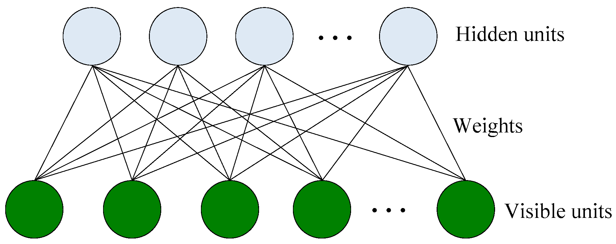
Figure 2.
An illustration of three-layer DBN with logistic regression.

Figure 3.
The maps of correlation coefficients of spectral bands in different datasets: (a) Indian Pines; (b) University of Pavia; and (c) Salinas.
Figure 3.
The maps of correlation coefficients of spectral bands in different datasets: (a) Indian Pines; (b) University of Pavia; and (c) Salinas.

Figure 4.
The correlation coefficients of adjacent spectral bands in different datasets: (a) Indian Pines; (b) University of Pavia; and (c) Salinas.
Figure 4.
The correlation coefficients of adjacent spectral bands in different datasets: (a) Indian Pines; (b) University of Pavia; and (c) Salinas.

Figure 5.
The procedure of band grouping and texture features enhancement.
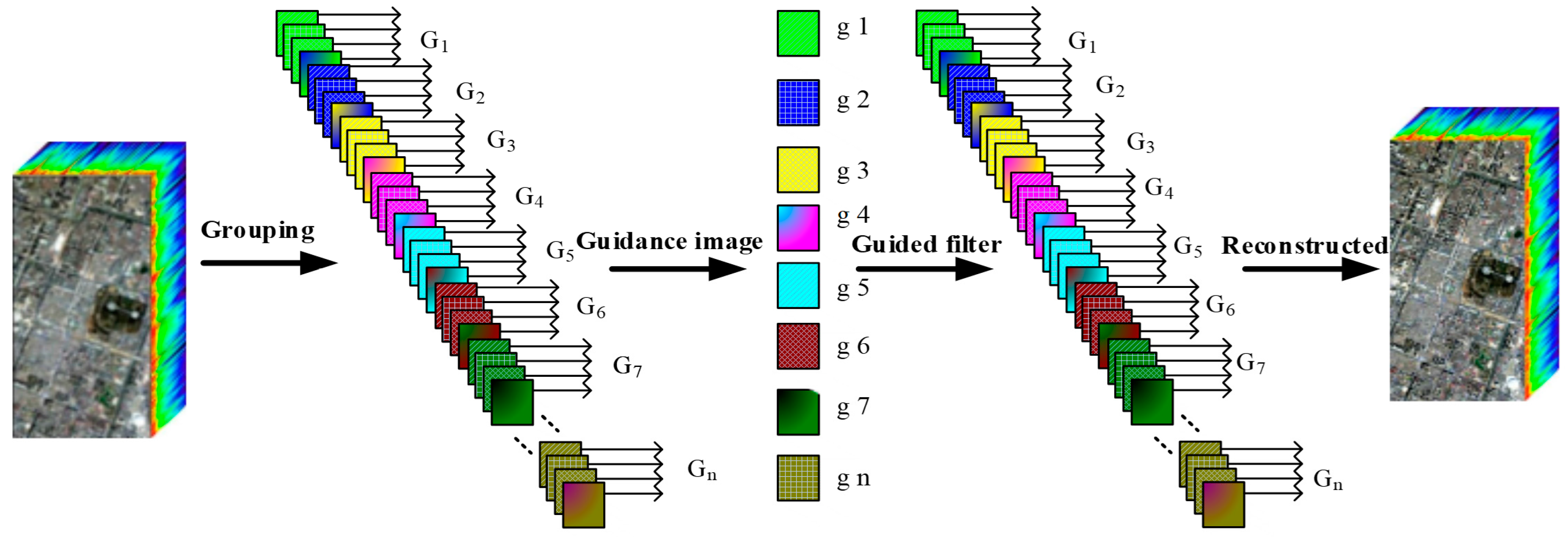
Figure 6.
Our proposed DBN network for classification.

Figure 7.
The relationship between accuracies and the number of hidden units in different datasets: (a) Indian Pines; (b) University of Pavia; and (c) Salinas.
Figure 7.
The relationship between accuracies and the number of hidden units in different datasets: (a) Indian Pines; (b) University of Pavia; and (c) Salinas.

Figure 8.
The relationship between accuracies and the learning rates in different datasets: (a) Indian Pines; (b) University of Pavia; and (c) Salinas.
Figure 8.
The relationship between accuracies and the learning rates in different datasets: (a) Indian Pines; (b) University of Pavia; and (c) Salinas.
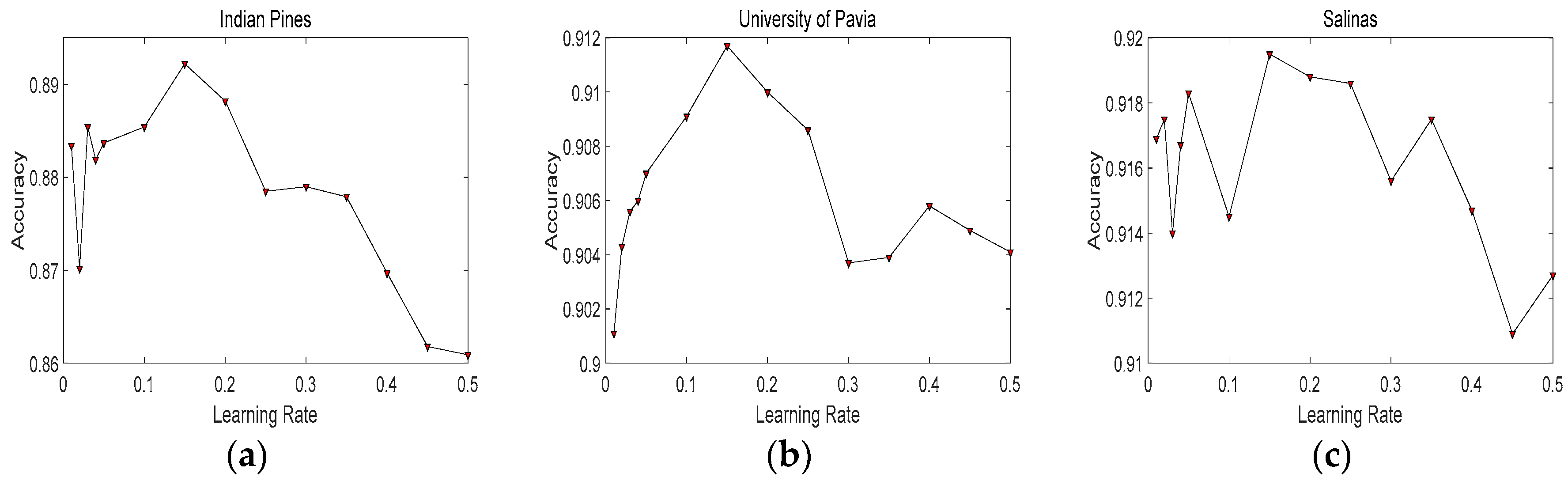
Figure 9.
The relationship between accuracies and the numbers of Max epoch in different datasets: (a) Indian Pines; (b) University of Pavia; and (c) Salinas.
Figure 9.
The relationship between accuracies and the numbers of Max epoch in different datasets: (a) Indian Pines; (b) University of Pavia; and (c) Salinas.
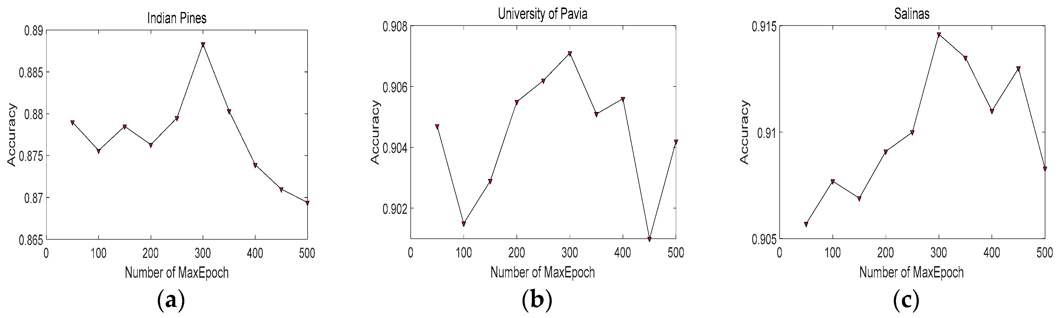
Figure 10.
P-class confusion matrix.

Figure 11.
The reconstructions of the border-pixels and inner-pixels of different classes in Indian Pines. First row is the reconstruction information of Class 2, second row is the reconstruction information of Class 4, third row is the reconstruction information of Class 6 and last row is the reconstruction information of Class 8.
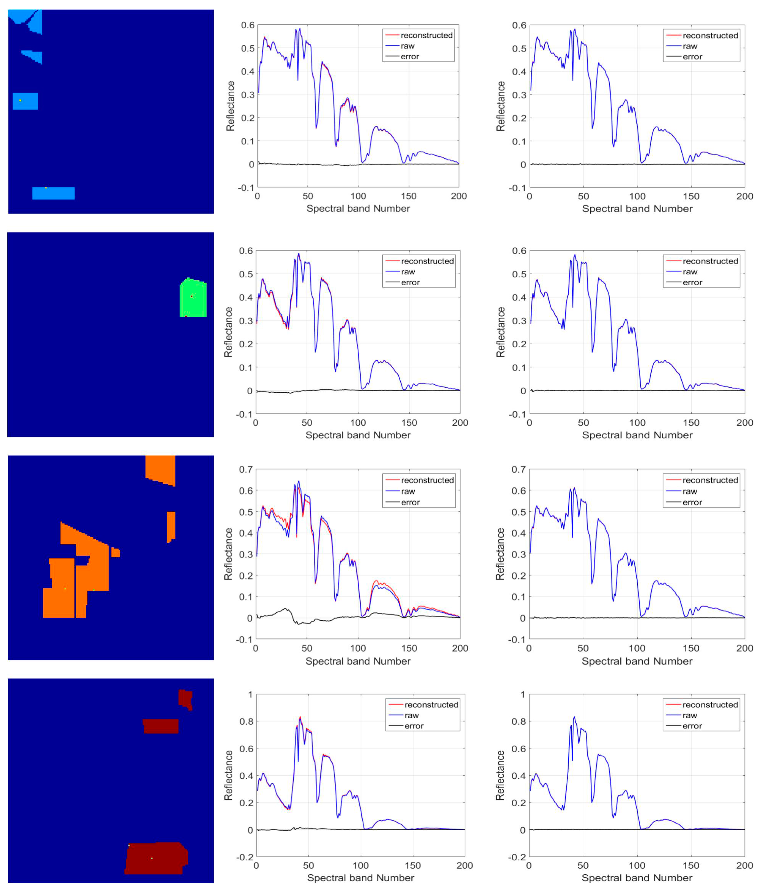
Figure 12.
The classification maps obtained via different algorithms in Indian Pines: (a) Ground truth; (b) SVM; (c) RBFNN; (d) O_DBN; (e) SVM_TFE; (f) RBFNN_TFE; (g) CNN; (h) EFP-G-c; and (i) the proposed framework.
Figure 12.
The classification maps obtained via different algorithms in Indian Pines: (a) Ground truth; (b) SVM; (c) RBFNN; (d) O_DBN; (e) SVM_TFE; (f) RBFNN_TFE; (g) CNN; (h) EFP-G-c; and (i) the proposed framework.
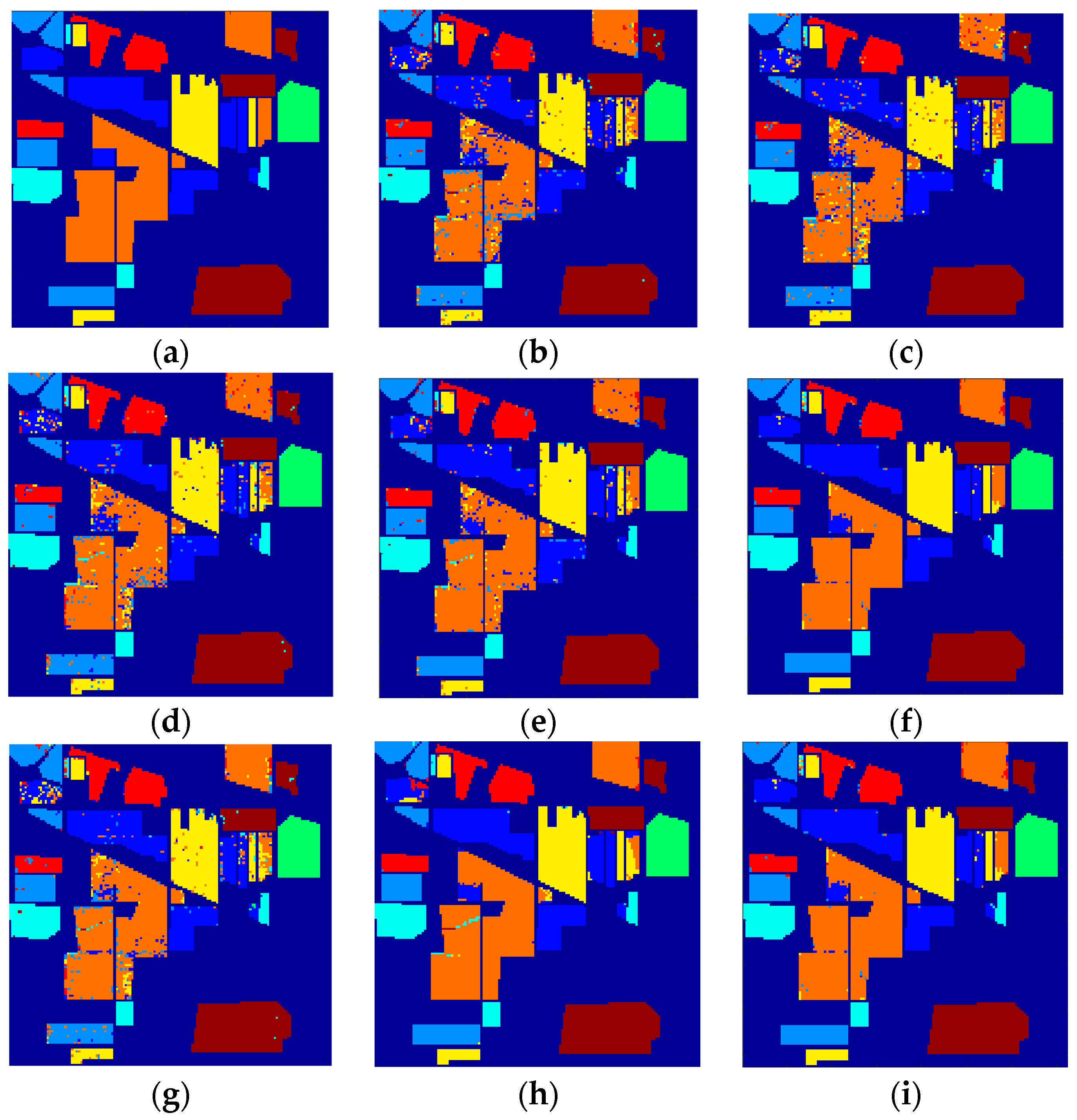
Figure 13.
The classification maps obtained via different algorithms in University of Pavia: (a) Ground truth, (b) SVM, (c) RBFNN, (d) O_DBN, (e) SVM_TFE, (f) RBFNN_TFE, (g) CNN, (h) EFP-G-c and (i) the proposed framework.
Figure 13.
The classification maps obtained via different algorithms in University of Pavia: (a) Ground truth, (b) SVM, (c) RBFNN, (d) O_DBN, (e) SVM_TFE, (f) RBFNN_TFE, (g) CNN, (h) EFP-G-c and (i) the proposed framework.
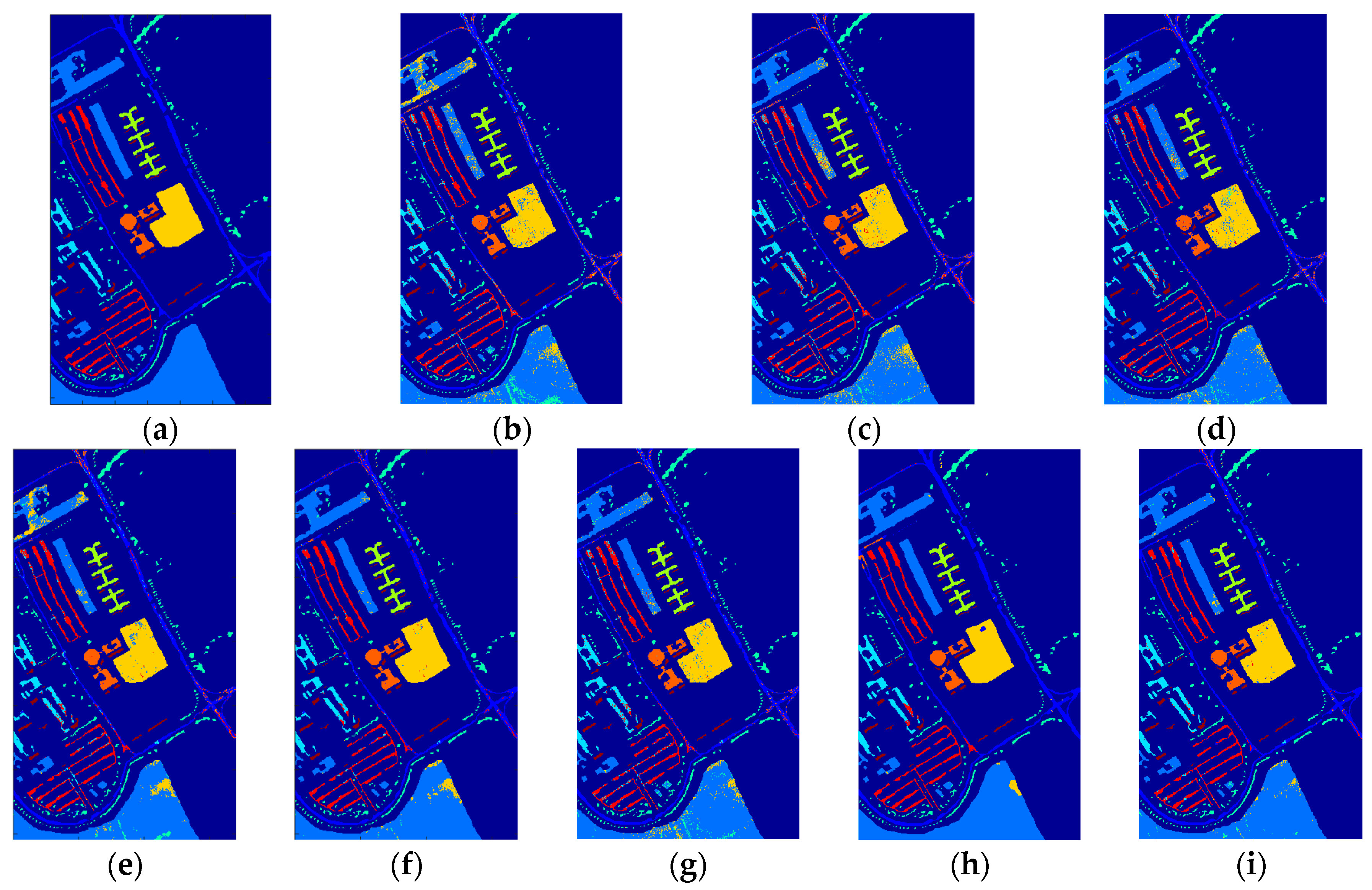
Figure 14.
The classification maps obtained via different algorithms in Salinas Dataset: (a) Ground truth, (b) SVM, (c) RBFNN, (d) O_DBN, (e) SVM_TFE, (f) RBFNN_TFE, (g) CNN, (h) EFP-G-c and (i) the proposed framework.
Figure 14.
The classification maps obtained via different algorithms in Salinas Dataset: (a) Ground truth, (b) SVM, (c) RBFNN, (d) O_DBN, (e) SVM_TFE, (f) RBFNN_TFE, (g) CNN, (h) EFP-G-c and (i) the proposed framework.


Table 1.
Feature calculated from the normalized co-occurrence matrix .
| No. | Feature | Formula |
|---|---|---|
| Energy | ||
| Entropy | ||
| Contrast | ||
| Mean | ||
| Homogeneity |
Table 2.
Number of training and testing samples used in the Indian Pines dataset.
| No. | Classes | Training | Testing |
|---|---|---|---|
| 1 | Corn-notill | 300 | 1160 |
| 2 | Corn-mintill | 300 | 534 |
| 3 | Grass-pasture | 300 | 197 |
| 4 | Hay-windrowed | 300 | 189 |
| 5 | Soybean-notill | 300 | 668 |
| 6 | Soybean-mintill | 300 | 2168 |
| 7 | Soybean-clean | 300 | 314 |
| 8 | Woods | 300 | 994 |
| Total | 2400 | 6224 |
Table 3.
Number of training and testing samples used in the Pavia University dataset.
| No. | Classes | Training | Testing |
|---|---|---|---|
| 1 | Asphalt | 300 | 6331 |
| 2 | Meadows | 300 | 18,349 |
| 3 | Gravel | 300 | 1799 |
| 4 | Trees | 300 | 2764 |
| 5 | Painted metal sheets | 300 | 1045 |
| 6 | Bare Soil | 300 | 4729 |
| 7 | Bitumen | 300 | 1030 |
| 8 | Self-Blocking Bricks | 300 | 3382 |
| 9 | Shadows | 300 | 647 |
| Total | 2700 | 40,076 |
Table 4.
Number of training and testing samples used in the Salinas dataset.
| No. | Classes | Training | Testing |
|---|---|---|---|
| 1 | Brocoli_green_weeds_1 | 300 | 1709 |
| 2 | Brocoli_green_weeds_2 | 300 | 3426 |
| 3 | Fallow | 300 | 1676 |
| 4 | Fallow_rough_plow | 300 | 1094 |
| 5 | Fallow_smooth | 300 | 2378 |
| 6 | Stubble | 300 | 3659 |
| 7 | Celery | 300 | 3279 |
| 8 | Grapes_untrained | 300 | 10,971 |
| 9 | Soil_vinyard_develop | 300 | 5903 |
| 10 | Corn_senesced_green_weeds | 300 | 2978 |
| 11 | Lettuce_romaine_4wk | 300 | 768 |
| 12 | Lettuce_romaine_5wk | 300 | 1627 |
| 13 | Lettuce_romaine_6wk | 300 | 616 |
| 14 | Lettuce_romaine_7wk | 300 | 770 |
| 15 | Vinyard_untrained | 300 | 6968 |
| 16 | Vinyard_vertical_trellis | 300 | 1507 |
| Total | 4800 | 49,329 |
Table 5.
The accuracies obtained via different numbers of hidden layers in DBN.
| Datasets | 1 Layer | 2 Layers | 3 Layers | 4 Layers |
|---|---|---|---|---|
| Indian Pines | 0.8919 | 0.8948 | 0.8892 | 0.8432 |
| University of Pavia | 0.9090 | 0.9123 | 0.9065 | 0.8994 |
| Salinas | 0.9123 | 0.9228 | 0.9104 | 0.9064 |
Table 6.
Classification accuracy of different algorithms on Indian Pines.
| Class | SVM | RBFNN | O_DBN | SVM_TFE | RBFNN_TFE | CNN | EPF-G-c | Our Proposed |
|---|---|---|---|---|---|---|---|---|
| 1 | 0.8578 | 0.8672 | 0.8562 | 0.9069 | 0.9638 | 0.9107 | 0.9757 | 0.9690 |
| 2 | 0.9251 | 0.9288 | 0.9532 | 0.9625 | 0.9944 | 0.7783 | 0.9736 | 0.9888 |
| 3 | 0.9391 | 0.9543 | 0.9594 | 0.9594 | 0.9949 | 0.8462 | 0.9314 | 0.9594 |
| 4 | 0.9841 | 1 | 0.9947 | 1 | 1 | 0.9793 | 0.9793 | 1 |
| 5 | 0.9162 | 0.9237 | 0.9172 | 0.9506 | 0.9910 | 0.7842 | 0.9268 | 0.9880 |
| 6 | 0.8054 | 0.7975 | 0.8189 | 0.8962 | 0.9553 | 0.9348 | 0.9855 | 0.9613 |
| 7 | 0.9363 | 0.9459 | 0.9490 | 0.9522 | 0.9809 | 0.8442 | 0.9873 | 0.9682 |
| 8 | 0.9940 | 0.9950 | 0.9909 | 1 | 1 | 0.9929 | 0.9881 | 1 |
| OA | 0.8837 | 0.8854 | 0.8948 | 0.9343 | 0.9751 | 0.8983 | 0.9754 | 0.9756 |
| AA | 0.9197 | 0.9265 | 0.9270 | 0.9535 | 0.9850 | 0.8838 | 0.9685 | 0.9793 |
| Kappa | 0.8559 | 0.8582 | 0.8617 | 0.9180 | 0.9688 | 0.8736 | 0.9692 | 0.9694 |
Table 7.
Classification precision of different algorithms on Indian Pines.
| Class | SVM | RBFNN | O_DBN | SVM_TFE | RBFNN_TFE | CNN | EPF-G-c | Our Proposed |
|---|---|---|---|---|---|---|---|---|
| 1 | 0.8585 | 0.8643 | 0.8563 | 0.9132 | 0.9646 | 0.8440 | 0.9474 | 0.9571 |
| 2 | 0.7577 | 0.7631 | 0.7496 | 0.8877 | 0.9620 | 0.9270 | 0.9606 | 0.9661 |
| 3 | 0.9113 | 0.9353 | 0.8400 | 0.8873 | 0.9849 | 0.9492 | 0.9645 | 0.9692 |
| 4 | 0.9688 | 0.9844 | 0.9495 | 0.9895 | 1 | 1.0000 | 1 | 1 |
| 5 | 0.7917 | 0.7434 | 0.8037 | 0.8675 | 0.9272 | 0.9087 | 0.965 | 0.9396 |
| 6 | 0.9307 | 0.9341 | 0.9417 | 0.9643 | 0.9862 | 0.8538 | 0.9686 | 0.9836 |
| 7 | 0.7861 | 0.8710 | 0.8466 | 0.8617 | 0.9716 | 0.9490 | 0.9936 | 0.9882 |
| 8 | 0.9930 | 0.9940 | 0.9970 | 0.9990 | 1 | 0.9909 | 1 | 1 |
| Precision | 0.8747 | 0.8862 | 0.8731 | 0.9213 | 0.9746 | 0.9278 | 0.9750 | 0.9755 |
Table 8.
Classification accuracy of different algorithms on University of Pavia.
| Class | SVM | RBFNN | O_DBN | SVM_TFE | RBFNN_TFE | CNN | EPF-G-c | Our Proposed |
|---|---|---|---|---|---|---|---|---|
| 1 | 0.7466 | 0.7733 | 0.8650 | 0.8534 | 0.9029 | 0.9758 | 0.9579 | 0.9458 |
| 2 | 0.8442 | 0.8980 | 0.9281 | 0.9058 | 0.9601 | 0.9832 | 0.9993 | 0.9728 |
| 3 | 0.8533 | 0.8377 | 0.8410 | 0.8922 | 0.9305 | 0.7795 | 0.9511 | 0.9550 |
| 4 | 0.9801 | 0.9602 | 0.9765 | 0.9772 | 0.9787 | 0.9096 | 0.9677 | 0.9881 |
| 5 | 0.9990 | 0.9990 | 0.9990 | 0.9981 | 0.9971 | 0.9830 | 0.9372 | 0.9990 |
| 6 | 0.9108 | 0.9492 | 0.9125 | 0.9558 | 0.9903 | 0.8153 | 0.9263 | 0.9873 |
| 7 | 0.9456 | 0.9583 | 0.8990 | 0.9544 | 0.9932 | 0.6680 | 0.9885 | 0.9893 |
| 8 | 0.8430 | 0.8628 | 0.8613 | 0.9101 | 0.9571 | 0.8562 | 0.9421 | 0.9438 |
| 9 | 1 | 1 | 0.9985 | 1 | 1 | 0.9985 | 0.9895 | 1.0000 |
| OA | 0.8555 | 0.8888 | 0.9123 | 0.9133 | 0.9568 | 0.9211 | 0.9671 | 0.9696 |
| AA | 0.9025 | 0.9154 | 0.9201 | 0.9385 | 0.9678 | 0.8855 | 0.9622 | 0.9757 |
| Kappa | 0.8103 | 0.8525 | 0.8824 | 0.8845 | 0.9418 | 0.8943 | 0.9590 | 0.9590 |
Table 9.
Classification precision of different algorithms on University of Pavia.
| Class | SVM | RBFNN | O_DBN | SVM_TFE | RBFNN_TFE | CNN | EPF-G-c | Our Proposed |
|---|---|---|---|---|---|---|---|---|
| 1 | 0.9795 | 0.9798 | 0.9675 | 0.9836 | 0.9877 | 0.8531 | 0.9822 | 0.9837 |
| 2 | 0.9720 | 0.9841 | 0.9763 | 0.9869 | 0.9980 | 0.9341 | 0.9756 | 0.9978 |
| 3 | 0.6657 | 0.6905 | 0.7568 | 0.7803 | 0.8876 | 0.8766 | 0.9711 | 0.9261 |
| 4 | 0.7657 | 0.8906 | 0.8207 | 0.9122 | 0.9808 | 0.9678 | 0.9642 | 0.9437 |
| 5 | 0.9831 | 0.9981 | 0.9849 | 0.9943 | 1 | 0.9981 | 0.9900 | 0.9877 |
| 6 | 0.6714 | 0.7388 | 0.7735 | 0.7456 | 0.8639 | 0.9484 | 0.9450 | 0.9189 |
| 7 | 0.5084 | 0.5583 | 0.6515 | 0.7567 | 0.8575 | 0.9592 | 0.9157 | 0.9586 |
| 8 | 0.8312 | 0.8028 | 0.8645 | 0.8394 | 0.8772 | 0.8752 | 0.9864 | 0.9117 |
| 9 | 1 | 1 | 0.9985 | 0.9985 | 1 | 0.9985 | 0.8779 | 0.9969 |
| Precision | 0.8197 | 0.8492 | 0.8660 | 0.8886 | 0.9392 | 0.9345 | 0.9565 | 0.9583 |
Table 10.
Classification accuracy of different algorithms on Salinas Dataset.
| Class | SVM | RBFNN | O_DBN | SVM_TFE | RBFNN_TFE | CNN | EPF-G-c | Our Proposed |
|---|---|---|---|---|---|---|---|---|
| 1 | 0.9965 | 0.9971 | 0.9947 | 0.9982 | 0.9988 | 1.0000 | 1.0000 | 0.9947 |
| 2 | 0.9947 | 0.9947 | 1 | 0.9956 | 0.9950 | 0.9933 | 0.9994 | 0.9962 |
| 3 | 0.9976 | 0.9988 | 0.9976 | 0.9976 | 0.9982 | 0.9589 | 0.9994 | 0.9976 |
| 4 | 0.9963 | 0.9963 | 0.9963 | 0.9954 | 0.9954 | 0.9838 | 0.9973 | 0.9973 |
| 5 | 0.9886 | 0.9849 | 0.9811 | 0.9874 | 0.9899 | 0.9898 | 0.9992 | 0.9853 |
| 6 | 0.9981 | 0.9986 | 0.9978 | 0.9981 | 0.9981 | 0.9995 | 0.9984 | 0.9973 |
| 7 | 0.9970 | 0.9963 | 0.9957 | 0.9960 | 0.9966 | 0.9988 | 0.9989 | 0.9963 |
| 8 | 0.8606 | 0.8567 | 0.8315 | 0.8761 | 0.8893 | 0.8379 | 0.8690 | 0.9085 |
| 9 | 0.9934 | 0.9985 | 0.9939 | 0.9942 | 0.9966 | 0.9896 | 0.9911 | 0.9949 |
| 10 | 0.9661 | 0.9758 | 0.9426 | 0.9698 | 0.9775 | 0.8848 | 0.9715 | 0.9614 |
| 11 | 0.9987 | 0.9961 | 0.9961 | 0.9987 | 0.9987 | 0.8919 | 1 | 1 |
| 12 | 0.9994 | 1 | 1 | 0.9994 | 1 | 0.9685 | 0.9992 | 0.9994 |
| 13 | 0.9968 | 0.9951 | 0.9984 | 0.9951 | 0.9951 | 0.9534 | 0.9987 | 0.9968 |
| 14 | 0.9792 | 0.9857 | 0.9948 | 0.9857 | 0.9805 | 0.9159 | 0.9978 | 0.9948 |
| 15 | 0.6972 | 0.7336 | 0.7646 | 0.7941 | 0.7916 | 0.7673 | 0.8856 | 0.9127 |
| 16 | 0.9920 | 0.9900 | 0.9854 | 0.9920 | 0.9914 | 0.9695 | 1 | 0.9887 |
| OA | 0.9212 | 0.9266 | 0.9228 | 0.9387 | 0.9421 | 0.9155 | 0.9543 | 0.9622 |
| AA | 0.9658 | 0.9687 | 0.9669 | 0.9733 | 0.9746 | 0.9439 | 0.9816 | 0.9826 |
| Kappa | 0.9114 | 0.9175 | 0.9133 | 0.9312 | 0.9350 | 0.9051 | 0.9486 | 0.9575 |
Table 11.
Classification precision of different algorithms on Salinas Dataset.
| Class | SVM | RBFNN | O_DBN | SVM_TFE | RBFNN_TFE | CNN | EPF-G-c | Our Proposed |
|---|---|---|---|---|---|---|---|---|
| 1 | 0.9988 | 0.9994 | 0.9971 | 0.9994 | 1 | 0.9801 | 1 | 1 |
| 2 | 0.9985 | 0.9985 | 0.9980 | 0.9994 | 0.9994 | 0.9947 | 0.9995 | 0.9991 |
| 3 | 0.9744 | 0.9721 | 0.9489 | 0.9830 | 0.9824 | 0.9976 | 0.9782 | 0.9682 |
| 4 | 0.9909 | 0.9864 | 0.9847 | 0.9918 | 0.9900 | 0.9973 | 0.9991 | 0.9900 |
| 5 | 0.9941 | 0.9970 | 0.9978 | 0.9920 | 0.9895 | 0.9315 | 0.9987 | 0.9924 |
| 6 | 0.9995 | 0.9997 | 0.9884 | 0.9992 | 0.9995 | 0.9978 | 0.9997 | 0.9940 |
| 7 | 0.9966 | 1 | 1 | 0.9951 | 1 | 0.9957 | 0.9991 | 0.9973 |
| 8 | 0.8209 | 0.8372 | 0.8592 | 0.8729 | 0.8726 | 0.8952 | 0.9162 | 0.9415 |
| 9 | 0.9956 | 0.9916 | 0.9898 | 0.9931 | 0.9927 | 0.9810 | 0.9475 | 0.9926 |
| 10 | 0.9517 | 0.9735 | 0.8699 | 0.9534 | 0.9674 | 0.9325 | 0.9627 | 0.9487 |
| 11 | 0.9808 | 0.9922 | 0.8242 | 0.9935 | 0.9948 | 0.9831 | 0.9994 | 0.9785 |
| 12 | 0.9909 | 0.9897 | 0.9748 | 0.9933 | 0.9921 | 1.0000 | 0.9987 | 0.9933 |
| 13 | 0.9777 | 0.9919 | 0.9935 | 0.9871 | 0.9839 | 0.9968 | 0.9920 | 0.9731 |
| 14 | 0.8737 | 0.9245 | 0.8235 | 0.9256 | 0.8945 | 0.9506 | 0.9359 | 0.8899 |
| 15 | 0.7803 | 0.7747 | 0.7344 | 0.8187 | 0.8341 | 0.5128 | 0.7777 | 0.8559 |
| 16 | 0.9701 | 0.9920 | 0.9861 | 0.9658 | 0.9953 | 0.9854 | 0.9946 | 0.9900 |
| Precision | 0.9559 | 0.9638 | 0.9356 | 0.9665 | 0.9680 | 0.9458 | 0.9687 | 0.9690 |
Table 12.
( values/Siginificant?) in the McNemar’s Test.
| Algorithms | Indian Pines | Pavia University | Salinas |
|---|---|---|---|
| SVM | 31.16/Yes | 68.33/Yes | 41.19/Yes |
| RBFNN | 31.34/Yes | 69.27/Yes | 41.39/Yes |
| O_DBN | 2.78/Yes | 3.74/Yes | 3.32/Yes |
| SVM_TFE | 31.95/Yes | 73.29/Yes | 41.21/Yes |
| RBFNN_TFE | 32.82/Yes | 74.84/Yes | 42.49/Yes |
| CNN | 3.50/Yes | 3.00/Yes | 4.49/Yes |
| EPF_G_c | 32.16/Yes | 75.13/Yes | 41.21/Yes |
Note: 5% significance level is selected.
© 2018 by the authors. Licensee MDPI, Basel, Switzerland. This article is an open access article distributed under the terms and conditions of the Creative Commons Attribution (CC BY) license (http://creativecommons.org/licenses/by/4.0/).
Share and Cite
MDPI and ACS Style
Li, J.; Xi, B.; Li, Y.; Du, Q.; Wang, K. Hyperspectral Classification Based on Texture Feature Enhancement and Deep Belief Networks. Remote Sens. 2018, 10, 396. https://doi.org/10.3390/rs10030396
AMA Style
Li J, Xi B, Li Y, Du Q, Wang K. Hyperspectral Classification Based on Texture Feature Enhancement and Deep Belief Networks. Remote Sensing. 2018; 10(3):396. https://doi.org/10.3390/rs10030396
Chicago/Turabian StyleLi, Jiaojiao, Bobo Xi, Yunsong Li, Qian Du, and Keyan Wang. 2018. "Hyperspectral Classification Based on Texture Feature Enhancement and Deep Belief Networks" Remote Sensing 10, no. 3: 396. https://doi.org/10.3390/rs10030396
Note that from the first issue of 2016, this journal uses article numbers instead of page numbers. See further details here.