Improving the Quality of Satellite Imagery Based on Ground-Truth Data from Rain Gauge Stations


1
Department of Statistics and Operations Research, Public University of Navarre, 31006 Pamplona, Spain
2
Institute for Advanced Materials (InaMat), Public University of Navarre, 31006 Pamplona, Spain
3
Department of Mathematics, UNED Pamplona, 31006 Pamplona, Spain
*
Author to whom correspondence should be addressed.
Remote Sens. 2018, 10(3), 398; https://doi.org/10.3390/rs10030398
Submission received: 22 December 2017
/
Revised: 11 February 2018
/
Accepted: 27 February 2018
/
Published: 5 March 2018
(This article belongs to the Special Issue Analysis of Multi-temporal Remote Sensing Images)
Abstract
:Multitemporal imagery is by and large geometrically and radiometrically accurate, but the residual noise arising from removal clouds and other atmospheric and electronic effects can produce outliers that must be mitigated to properly exploit the remote sensing information. In this study, we show how ground-truth data from rain gauge stations can improve the quality of satellite imagery. To this end, a simulation study is conducted wherein different sizes of outlier outbreaks are spread and randomly introduced in the normalized difference vegetation index (NDVI) and the day and night land surface temperature (LST) of composite images from Navarre (Spain) between 2011 and 2015. To remove outliers, a new method called thin-plate splines with covariates (TpsWc) is proposed. This method consists of smoothing the median anomalies with a thin-plate spline model, whereby transformed ground-truth data are the external covariates of the model. The performance of the proposed method is measured with the square root of the mean square error (RMSE), calculated as the root of the pixel-by-pixel mean square differences between the original data and the predicted data with the TpsWc model and with a state-space model with and without covariates. The study shows that the use of ground-truth data reduces the RMSE in both the TpsWc model and the state-space model used for comparison purposes. The new method successfully removes the abnormal data while preserving the phenology of the raw data. The RMSE reduction percentage varies according to the derived variables (NDVI or LST), but reductions of up to 20% are achieved with the new proposal.

1. Introduction
The presence of clouds, atmospheric absorption, weather effects and sensor-introduced noise can be important causes of distorted and missing data in satellite imagery. Therefore, numerous gap-filling and smoothing techniques have been developed in the past few years. Next, we cite some of these techniques. Timesat [1,2] and Hants [3] are very popular because of their good performance and free access. Both methods are mathematical procedures based on filtering and harmonic analysis and use multitemporal imagery for filling gaps, but do not use external auxiliary information. These approaches can be applied to long series of data and smooth complete series of images without any prior specification of the gaps to be filled. The moving weighted harmonic analysis (MWHA) [4] is another method based on a modification of the previous cited Hants technique that incorporates a moving support domain to assign the weights for all the points, therein greatly simplifying the determination of the frequency number. The spatially- and temporally-weighted regression (STWR) method [5] is more strongly focused on filling cloud gaps. This approach requires a one-by-one identification of the gaps and utilizes a simple least-squares linear regression to capture the temporal trends characterizing invariant similar pixels. Vuolo et al. [6] developed a proposal for smoothing and gap-filling high-resolution multi-spectral time series using the Whittaker smoother and derived information about the neighborhood. Gapfill [7] is a recent alternative that uses specific ordering among images and quantile regression for the gap-filling process. This technique achieves a great performance because it produces smoothed images of high quality; however, it is slow when filling large gaps, and it needs a prior specification of the gaps to be filled.
The MODIS and LANDSAT missions are carrying out similar programs for processing common remote sensing data derived from multi-temporal series of images in a routine manner. The normalized difference vegetation index (NDVI) and the day and night land surface temperature (LST) are two examples of such data. Smoothing NDVI is frequently conducted with the maximum value composite (MVC) procedure [8]. It assigns the maximum value of the time series of pixels across the composite period. Alternative techniques include the use of a bidirectional reflectance distribution function (BRDF-C), the constrained maximum value composite (CV-MVC) [9], the mean value iteration filter (MVI), the changing-weight filter (CW) and the interpolation for data reconstruction (IDR) technique [10]. For day and night LST, it is common to average the cloud-free pixels over the composite period [11]. Composite images are then of weekly or biweekly temporal resolution. However, even after the composition process, residual noise can still arise in images, and therefore, a smoothing procedure using high-spatio-temporal-resolution ground-truth data is proposed in this paper. Frequently, remote sensing data are proxy variables in mathematical or statistical models for improving the predictions of ground-truth data. For example, land surface temperature from MODIS MOD11A2 was used as a proxy variable in a spatio-temporal regression model for smoothing temperatures in Croatia [12], but used a reduced number of images and rain gauge stations. To improve the estimation of the area occupied by olive trees, a unit level linear mixed model was proposed, whereby the auxiliary variable came from multispectral Landsat 7 ETM images [13]. Different geostatistical models were checked with soil data collected with automated sensor networks to provide the spatio-temporal interpolation of soil water, temperature and electrical conductivity in the Cook Agronomy Farm dataset [14]. A distributed lag model for assessing the impact of current and previous 16-day rainfall anomalies was proposed based on the enhanced vegetation index as a proxy for above-ground net productivity in South Africa [15]. A complete reconstruction of time series of daily LST data in central Europe from 2003 to 2016 was achieved in [16], where remote sensing emissivity and elevation were used as external covariates in the spatio-temporal interpolation process. The authors used air temperature ground-truth data to check the predicted values. In this case, various remote sensing data were the explanatory variables of the models used for improving the predictions in other remote sensing data. Research wherein ground-truth data are used as proxy variables wherein remote sensing data including the target variable are more scarce. Only recently, we have found a cubic spline model that has been combined with a weighted least squares regression [17] for extracting the seasonality characterizing the land surface temperature and a space-state model (SSM) that has been introduced for detecting changes in trends of surfaces occupied by different categories of NDVI in continental Spain during 2011, 2012, and 2013 [18].
In this work, we propose to merge multi-temporal remote sensing data with ground-truth data using a thin plate spline smoothing method with external auxiliary variables. Thin plate splines can be seen as a generalization of a regression model wherein the linear relationship between the response variable and the coordinates is substituted by a non-parametric function providing a more flexible fitting [19]. Under certain conditions, the thin-plate splines are formally equivalent to kriging [20], and because the measure of smoothness is invariant under the rotation of the coordinates, thin-plate splines are specially suited for spatial data. The thin-plate splines have an important advantage with regard to universal kriging because they do not need to fit variograms. Moreover, the estimators of the thin-plane splines can be obtained in a closed form by solving a linear system of n equations, where n is the number of data points. The approach used here is based on fitting second-order splines to the anomalies obtained from the median of the target gap image neighborhood, therein using the temporal and spatial dependences of the previous and subsequent images across different years for smoothing potential outliers. Using only the coordinates, but without external covariates, the performance of thin-plate splines for filling gaps was evaluated in a simulation study, which showed that this technique is faster and more accurate than Timesat, Hants and Gapfill when filling different sizes of gaps in day and night LST and is equally competitive when filling NDVI gaps [21]. Here, we improve this proposed method by including auxiliary variables from ground-truth data, which must be fitted at the same spatio-temporal resolution as remote sensing data. We also focus on smoothing outliers instead of filling gaps, and we compare the performance of the newly-proposed method with a spatio-temporal state-space model using the same ground-truth data. We check the performance through a simulation study whereby time series of three different remote sensing datasets are altered and later smoothed with these models.
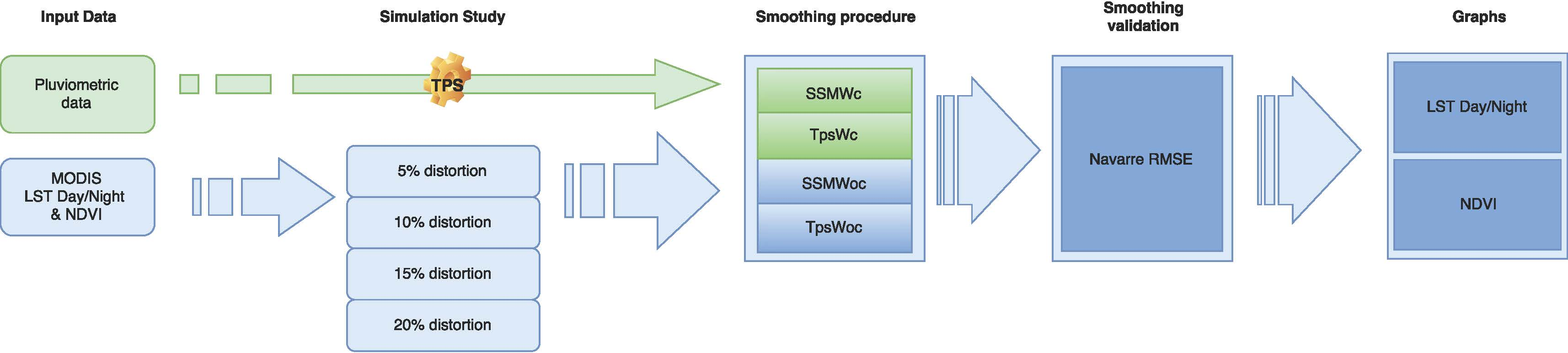
Figure 1 shows the flowchart of the paper. First, meteorological and remote sensing data are taken. Second, daily ground-truth information needs to be averaged over eight- and 16-day periods to match the corresponding day and night LST and NDVI time periods. These data are interpolated in the study region of Navarre (Spain) (see Figure 2) through a thin-plate spline model with altitude as the external covariate. This is a preliminary task because these data are a small discrete set, and greater spatial resolution is recommended for predicting. For the simulation study, remote sensing data are altered with different sizes of distortions, i.e., 5%, 10%, 15% and 20%, and different magnitudes are used according to the derived variables. Third, we fit different models for every outlier outbreak: a state-space model with covariates (SSMWc), a thin-plate spline model with covariates (TpsWc), a state-space model without covariates (SSMWoc) and a thin-plate spline model without covariates (TpsWoc). All of these methods provide multi-temporal smoothed series of the three remote sensing datasets. Finally, to compare model performances, we obtain the square root of the mean squared prediction error, which will be summarized in graphs and tables.
2. Data
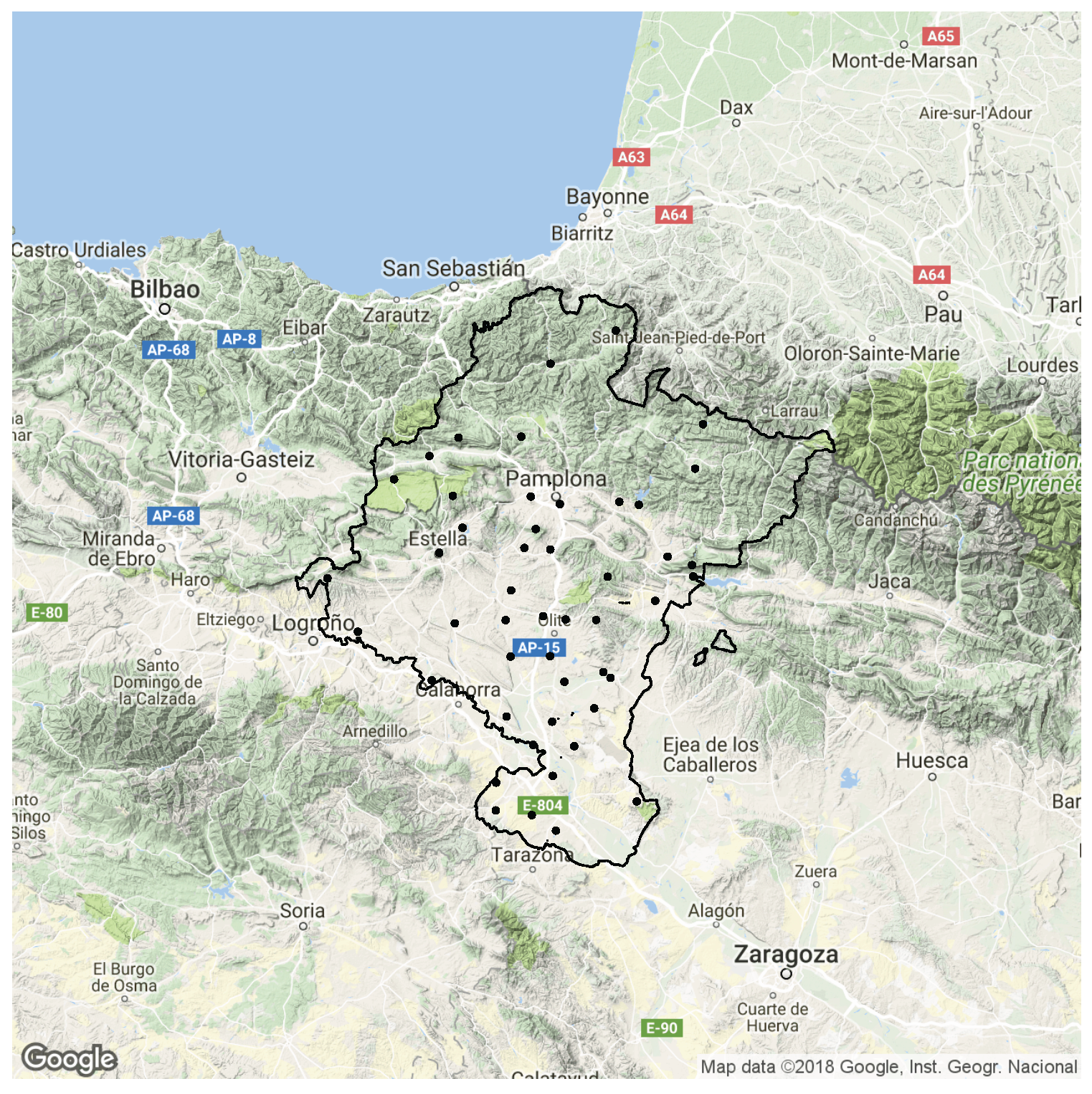
Navarre is a region of approximately 10,000 km located in the north of Spain (see Figure 2). Elevations vary between 200 and 2500 meters in the highest zone of the Pyrenees, located in Northeastern Navarre. Valleys and mountains are ubiquitous in the north, and small hills are common in the central part of the province. The northwest of Navarre is humid, but not highly so, and the northeast is a mountainous region with elevations between 1459 m and 2438. The central area is characterized by a temperate Mediterranean climate, with a tendency towards a continental climate. The south is mainly flat; the climate is Mediterranean and continental with dry summers; temperatures exhibit large annual variations; there is minimal and irregular rainfall; and northerly winds are frequent. Clearly, the climate varies across the province, and large weather differences can be experienced on the same day.
In this study, we have drawn classical variables, such as the maximum temperature and humidity, from 48 rain gauge stations. The data are of daily temporal resolution, from which weekly and biweekly mean data are derived. The average distance among rain gauge stations is approximately 15 km.
The Moderate Resolution Imaging Spectroradiometer (MODIS) provided the day and night LST composite images from Version-5 MOD11A2 (Terra) and the NDVI composite images from both Version-5 MOD13A2 (Terra) and Version-5 MYD13A2 (Aqua); see the URL [9] for details. We have focused on composite images of the Navarre region from the 2011 to 2015 time period. Each of the day LST and night LST remote sensing datasets require 230 tiles for enclosing Navarre. These datasets correspond to 46 scenes with a temporal resolution of 8 days every year for 5 years. Terra and Aqua have different starting dates each year because Terra starts on the first day of January and Aqua starts on the ninth day of January. Therefore, to achieve two composite NDVI images per month every year, we have retrieved 23 images from Aqua and one image from Terra, fitted to November. In total, 120 scenes with a 16-day temporal resolution have been captured across 5 years of study. The spatial resolution of each tile is equal to (25,564) pixels of approximately 1 km. Inside the Navarre borders, 11,691 pixels are enclosed. All images have been downloaded from [22] in Hierarchical Data Format (HDF). This format helps catalog geo-referenced images, but makes data processing more difficult. Then, all images were transformed into TIFF format to be processed by the R software [23].
NDVI is a very useful index for agricultural mapping, yield monitoring and measuring changes in ecosystems, land use and climate at both global and regional scales [24,25,26]. It is obtained in two important bands, the red (R) and near-infrared (NIR), and is calculated as [27]. NDVI has a theoretical maximum of one, and its relationship to vegetation characteristics, such as biomass, productivity, percent cover and leaf area index, is asymptotically nonlinear as it approaches one. NDVI is less sensitive to ground characteristics at higher values and essentially saturates when the leaf area index is greater than one [28]. Barren land, sand and snow usually present very low NDVI values, and sparse vegetation presents values of approximately between 0.2 and 0.5. High NDVI values, roughly from 0.6 to 0.9, correspond to dense vegetation from crops at their peak growth stage and tropical vegetation.
The MODIS LST product is derived from two thermal infrared (TIR) channels: 31 (10.78 to 11.28 m) and 32 (11.77 to 12.27 m). More information can be found in [29]. Assuming that the signal difference in the two TIR bands is caused by differential absorption of radiation in the atmosphere, the correction of atmospheric effects is performed with the split-window algorithm [30]. Using prior knowledge of the land cover type classification based on the MODIS land cover product (MOD12C1), this algorithm corrects for emissivity effects. Uncertainty in LST estimates increases when significant variations in temperature occur at the 5-km scale [31]. Errors in LST retrieval may be larger in bare soil and highly heterogeneous areas due to large uncertainties in surface emissivities and when the column water vapor content is high [31]. An eight-day composite period was chosen because twice this period is the exact ground track repeat period of the Terra platform. LST over eight days is the averaged LSTs of the MOD11A2 product for eight days. Processing these images will preserve the original temperature in Kelvin, but the day and night LST figures given in this work will be expressed in Celsius.
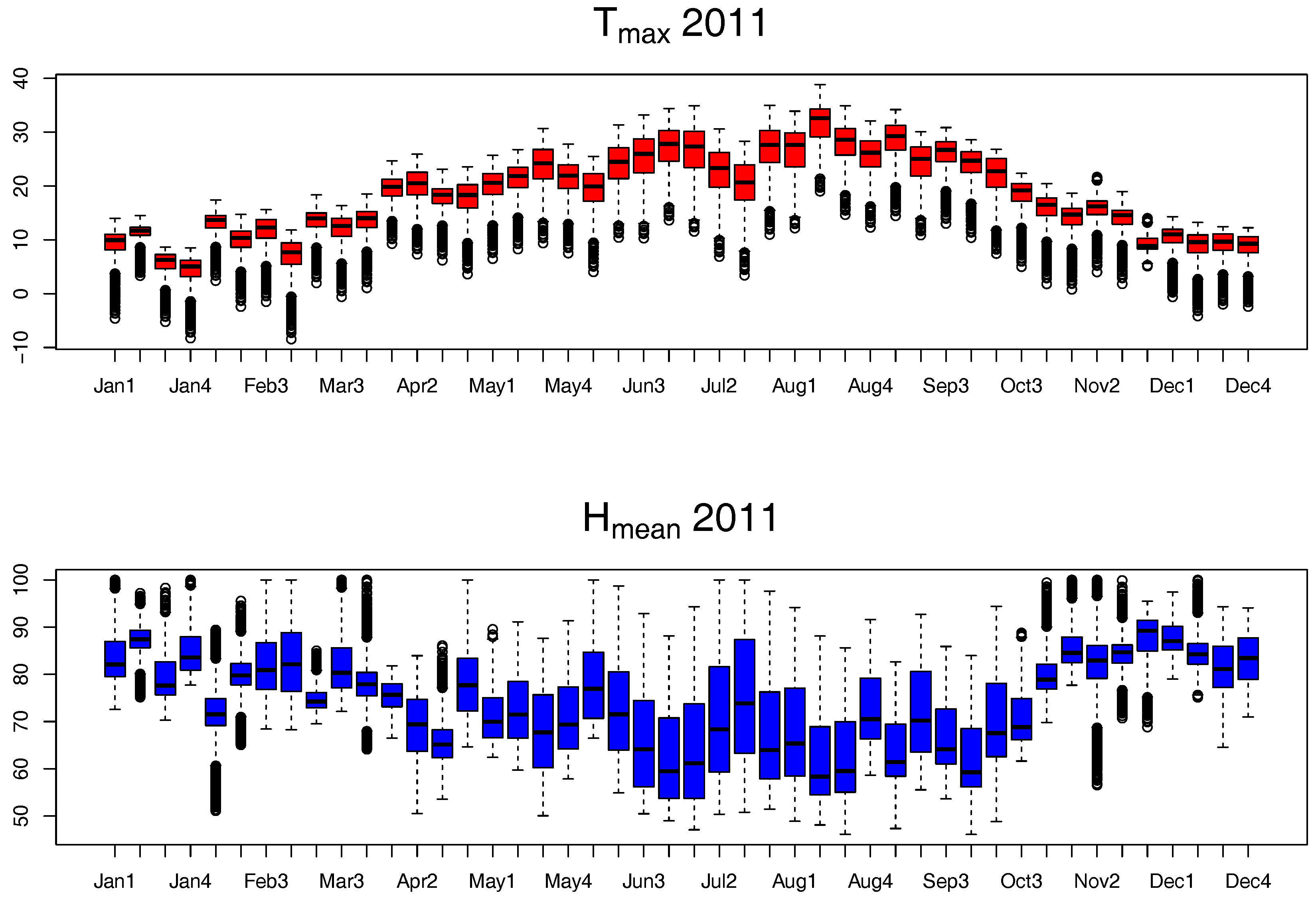
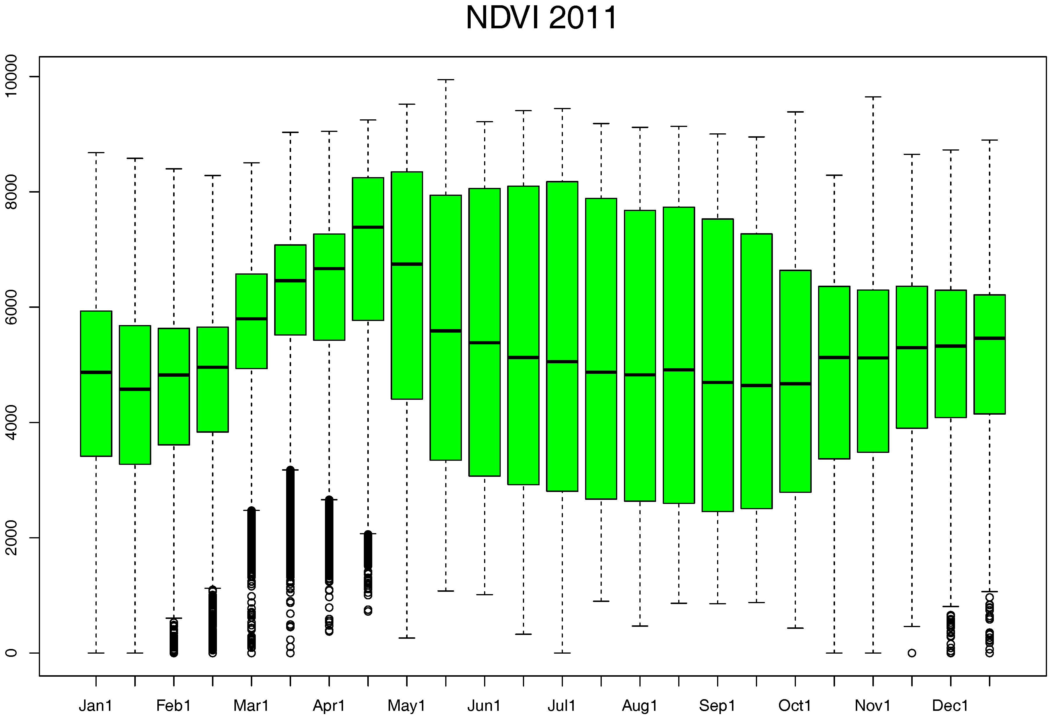
Both derived variables come from composite images, meaning that they have been pre-processed to reduce noise coming from atmospheric and electronic effects and that their accuracy has also been checked via ground-truth data at a coarse spatial resolution. However, when downscaling these data to small regions and comparing them with ground-truth data, we can observe, in some seasons, typically in autumn and winter, some abnormal results. Figure 3 shows from the top to bottom the boxplots of the day LST and night LST remote sensing data and those of the mean maximum temperature () and the mean humidity () in Navarre during 2011 for 46 time periods. Each boxplot depicts the median in the horizontal line and the dispersion of every image in a particular stage. Within each box, data between the first and third quantiles are plotted. Dots outside vertical extensions might be, but are not necessarily outliers. The meteorological variables and have been chosen because they are the most highly correlated with day and night LST and NDVI during the time periods. Figure 4 shows the boxplots of NDVI in the 24 time periods of 2011. In Figure 3 and Figure 4, all the variables show a clear pattern of seasonality, yet in , larger variability is observed. Day and night LST and show a parallel concave shape and therefore a positive correlation across time periods; is more convex, showing a negative correlation with day and night LST. NDVI presents a different seasonality pattern, which is negatively correlated with and positively correlated with across the time periods. In summer, all the variables are more stable and show less variability. Similar phenology patterns are found across the study period of 2011- to 2015.
Figure 5 shows Navarre images in the third week of 2011. At the top, day LST and (in Celsius) are shown, and at the bottom, night LST (in Celsius) and (in percentages) are presented. We can also see the large similarity among these patterns on these dates. The dots on the right images correspond to the rain gauge stations used as ground-truth data. Figure 6 shows the altitude of Navarre and the NDVI on the second fortnight of February 2014 because NDVI includes 24 periods. In this figure, we can also check why similar patterns correspond to a high correlation.
3. Methods
Filling gaps and removing abnormal observations in satellite imagery are traditionally performed by mathematical or statistical procedures based on modeling similarities of the same historical series of images. Few methods use external information. The newly-proposed method in this paper, named TpsWc, uses additional auxiliary data from external sources, and it is compared with a state-space model that uses the same auxiliary variables or covariates.
3.1. The Thin-Plate Spline Model with Covariates
First, we fix the target image to be smoothed and define its neighborhood. Let us assume that we have an day LST target image. In this case, images are available every year from (), which should be arranged into a matrix, where the rows of the matrix correspond to different years. In the NDVI case, images are available each year; they should be arranged into a matrix. All the images in the same column correspond to the same time period, but different years. They share a neighbor composed of this column and the previous and subsequent columns of images; therefore, the neighbor of every target image consists of 15 images. In the first time period of 2011 and in the last time period of 2015, previous and subsequent images are also needed, but they do not correspond to the years under study. The second step of this procedure is to compute the median image out of those 15 images and obtain the corresponding anomalies for the target image. The anomalies could come from the mean or median. It is more convenient to calculate them from the mean in the gap-filling process because the mean can be obtained without missing values; calculating from the median should be performed when smoothing altered pixels, because it is more robust, and we are likely not aware of altered pixels.
In greater detail, let us denote as the derived variable in location , , where 25,564 is the total number of pixels in the target image for year r. Then, the -th pixel of the median image of time g across the years is defined over the 15 images involved in its neighborhood, i.e.,
and the anomalies are obtained as the differences between the original values and the median:
Next, a thin-plate spline model (Tps) is applied to a 5-times lower resolution of the anomalies inside Navarre obtained through a median aggregation. Therefore, the median can be calculated within the tile of 25,564 pixels, but the model will be constrained to the 11,691 pixels inside Navarre because that is where we possess ground-truth data. The reduction factor is recommended because it speeds up the running process and facilitates the previous image smoothing, but this can vary depending on the computer speed and memory. The thin-plate spline additive model for every image in a fixed time period g and year r with covariates is expressed as a non-parametric function of the coordinates plus the sum of three transformed external covariates: the altitude , maximum mean temperature and mean humidity . Then,
where is the vector of locations, is a non-parametric function of the coordinates and are the model coefficients associated with the covariates. They need to be estimated from the data because, later, we will be able to calculate the smoothed images. For every year r and stage g, is the vector of remote sensing anomalies, and () are the transformed covariates of their original covariates: altitude , maximum temperature and mean humidity .
This transformation is needed to preserve the correlation between the response variable calculated as median anomalies of the remote sensing data and the transformed covariates of , and altitude. This is because day LST, night LST and NDVI remote sensing data are correlated with , and altitude, respectively, but their anomalies are not necessarily correlated with these. Therefore, a simple transformation that consists of subtracting the remote sensing median from the covariates is needed. The error vector has zero mean and variance . The thin-plate spline prediction is obtained as a weighted average of the observed data because the optimal estimate is linear in the observations. Finally, the predictions are computed over the pixels of the original resolution. Model (3) with covariates (TpsWc) and without covariates (TpsWoc) is run for all time periods, the three remote sensing datasets and the four sizes of distortions for the simulation study. The R package fields [32] estimates second-order thin-plate spline models by fitting a surface to irregularly-spaced data.
3.2. The State-Space Model with Covariates
This model is a stochastic spatio-temporal model (SSM) [33] widely used for dynamical systems [18,34,35]. The model includes two equations: the transition Equation (4) and the state Equation (5). The first equation explains a linear regression between the response variable and the covariates. In this example, the response variable is the remote sensing data (day and night LST and NDVI), and the covariates are the meteorological variables , and altitude. The second equation expresses the temporal dependence. The stochastic process at locations and time points is represented by , where can be day and night LST or NDVI, and . The value of depends on both the remote sensing data and the m-th climatological season. In winter (January, February and March) and summer (July, August and September), there are day and night LST composite images, and in spring (April, May and June) and fall (October, November and December), there are day and night LST composite images. When using NDVI, there are images in each climatological season.
In this application, we consider locations obtained by defining a km grid inside Navarre. The state-space model with covariates (SSMWc) is given by:
where now are the model coefficients to be estimated. The first covariate is time invariant and corresponds to the altitude of the gridded locations. The remainder of the covariates, and , are the spatio-temporal meteorological covariates: maximum temperature () and mean humidity () depending on the location s and time t. The unobservable latent temporal process, , considers the temporal dynamics of data through an autoregressive process. This means that the current state depends on the previous state in the state equation through a transition matrix G. The initial state vector is assumed to be normally distributed with mean and covariance .
This state-space model is fitted in the R statistical software using the Stem package [36]. In this application, state-space models with covariates (SSMWc) and without covariates (SSMWoc) are estimated for the three remote sensing datasets, the four types of outlier outbreaks and all images between 2011 and 2015.
4. Results and Discussion
To check the contribution of the ground-truth data for improving the quality of satellite imagery, a simulation study is conducted in Navarra using 120 composite images of NDVI, 230 composite images of day LST and 230 composite images of night LST between 2011 and 2015. In this simulation study, we randomly include four different sizes of outlier outbreaks with and abnormal observations in each image. The distortion consists of altering 50% of the NDVI raw data, 5% of the day LST raw data and 5% of the night LST raw data. The distortion percentages look different, but all represent approximately 50% of the range of the three remote sensing datasets used in this paper. The performance of the methods is evaluated with the square root of the mean squared prediction error, defined by:
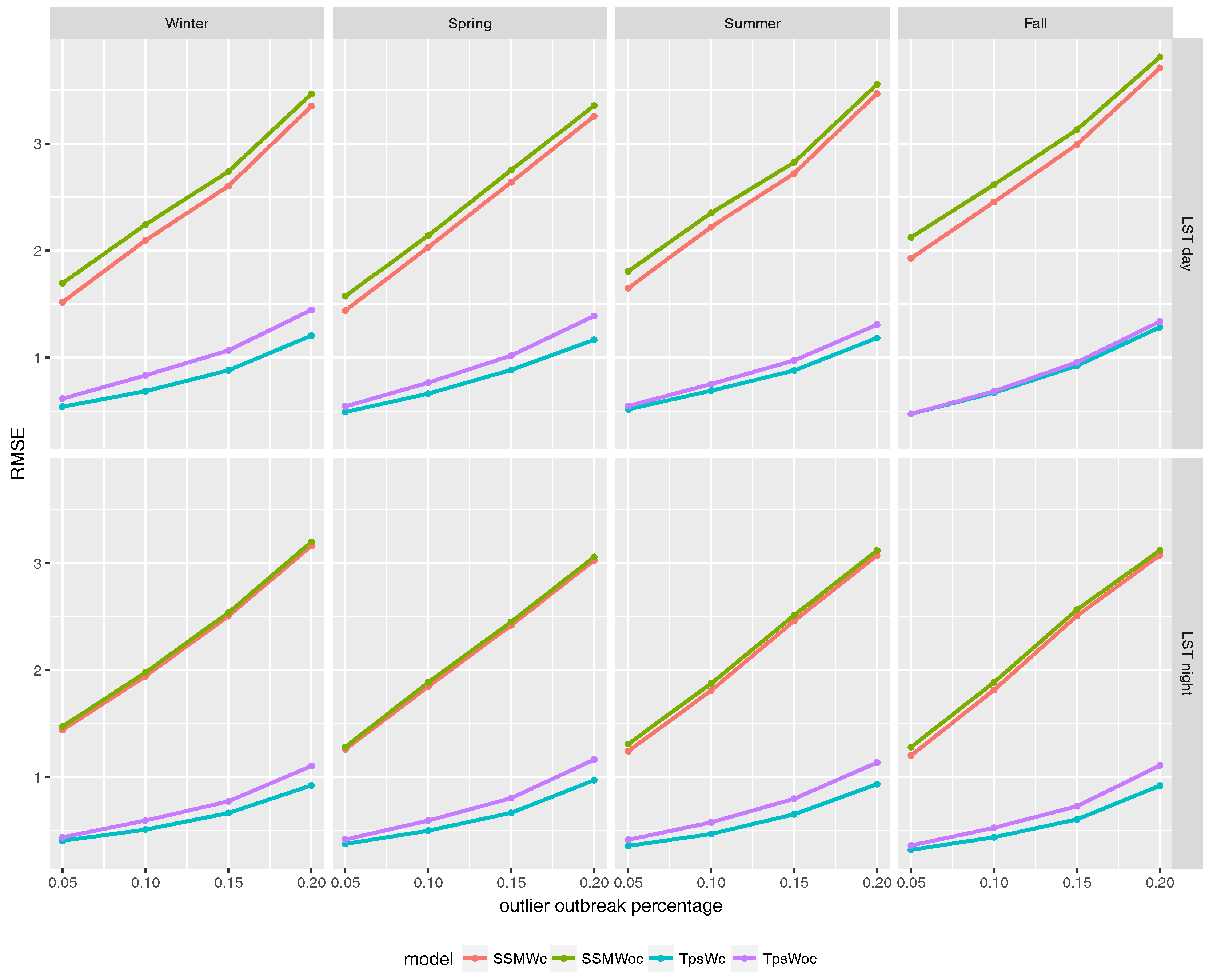
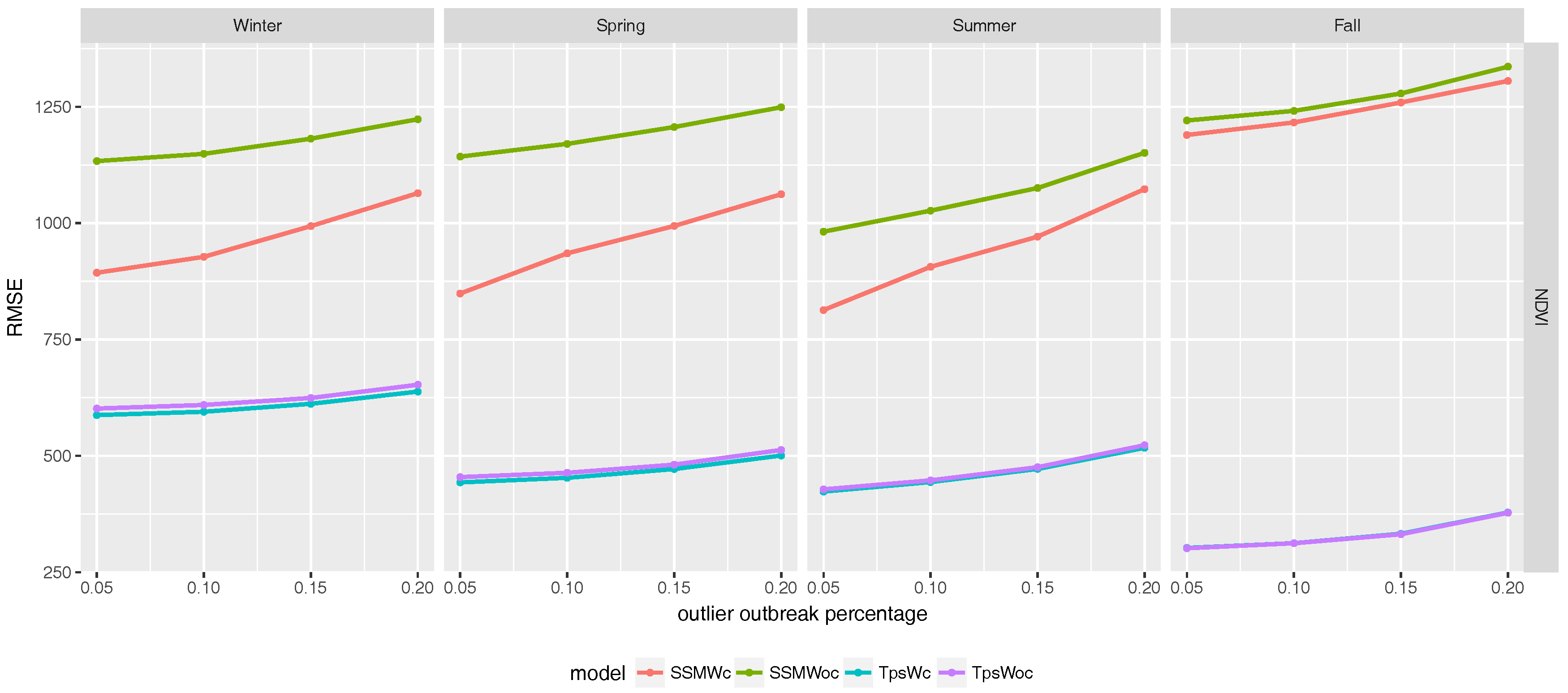
where and are the original and predicted derived variables, respectively; 11,691 is the number of pixels inside the Navarre borders; and is the number of images in the m-th climatological season across the five years (see Section 3.2). The index indicates the type of model; k is the type of distortion; and l is the type of derived variable. is calculated and plotted in Figure 7 and Figure 8. Figure 7 depicts the RMSE of day LST and night LST for the two versions of Tps, i.e., TpsWc (blue with covariates) and TpsWoc (purple without covariates), and SSM, i.e., SSMWc (red with covariates) and SSMWoc (green without covariates). In all cases, TpsWc outperforms the remaining models, as it achieves the lowest RMSE. Figure 8 shows the RMSE obtained after smoothing NDVI. TpsWc is again the best method in all the climatological seasons and again presents a greater difference with regard to the SSM with and without covariates (SSMWc and SSMWoc). Nevertheless, differences between thin-plate splines with and without covariates are apparently less important than in day LST and night LST, but only because the range of the NDVI variable is smaller than that of LST. Summarizing, all the figures show lower RMSE when using covariates in both thin-plate splines (Tps) and state-space models (SSM). Table 1 shows the RMSE reduction percentage when both models include ground-truth information compared to when not including this information. The maximum percentage reduction is approximately 20% in night LST for TpsWc and in NDVI for SSMWc; however, TpsWc clearly provides the lowest values of RMSE with and without covariates.
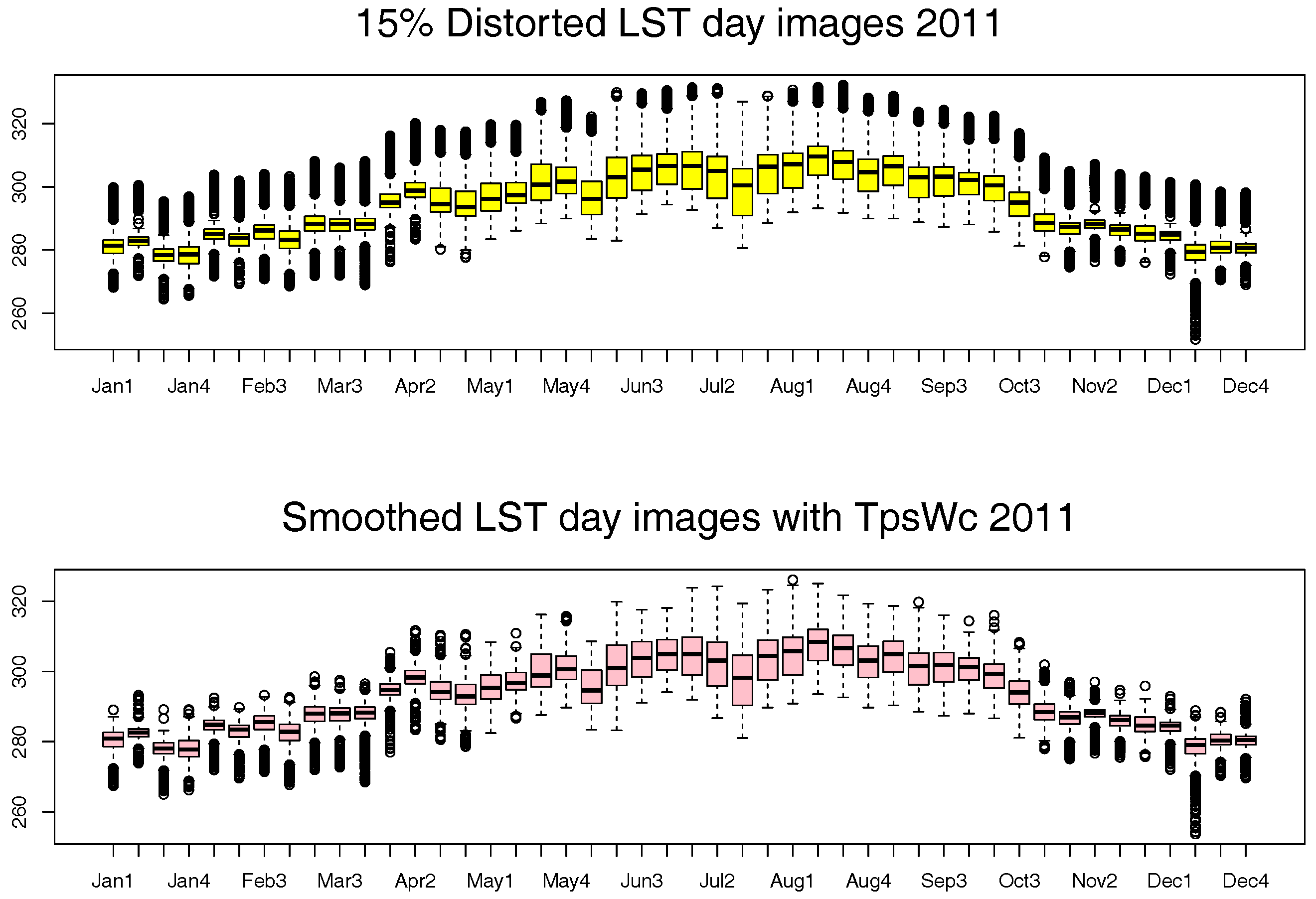
Figure 9 shows the effects of distorting the images and smoothing them in the fourth time period of November 2011. At the top and from left to right, we see the distorted image of LST with an outlier outbreak of 5%, the TpsWc smoothed image and the SSMWc smoothed image with altitude, and as the ground-truth covariates. At the bottom, the distorted image with an outlier outbreak of 20% in the same time period and the derived smoothed images are shown. Both models remove distorted data, and SSMWc seemingly better smooths the images, but TpsWc better preserves the original image pattern. The top of Figure 10 shows the boxplots of the distorted images, and at the bottom, the boxplots of the smoothed images in the 46 periods of 2011 are shown. We can see how the phenology of the remote sensing data is preserved after smoothing.
The simulation study shows an important decrease in the RMSE calculated with both the TpsWc and SSMWc methods; however, unless we alter the ground-truth data, we cannot evaluate what occurs in terms of RMSE when the covariates exhibit higher or lower correlations with the dependent variable. This is why we have defined a new artificial covariate linearly correlated with the remote sensing data. This correlation takes on values of and 1. After introducing at random 20% abnormal observations in the time series of raw images, we smoothed them using TpsWc and SSMWc with the artificial covariate. When the correlation increases, a greater reduction in the RMSE is observed, although specific values are not shown here to preserve space. On average, each time we increase the linear correlation of the artificial variable with the remote sensing data by one tenth, a 3 to 4% RMSE reduction in the TpsWc and SSMWc models is observed. Therefore, using ground-truth data for increasing the quality of composite images is a recommended option in both models, although TpsWc achieves better results, as it has the lowest RMSE. The mean running time of day and night LST for processing 230 images is approximately 13 min with TpsWc and 11 min with SSWc on a PC with an Intel Core i7-4790 (Intel Corporation, Santa Clara, CA, USA) 3.60 GHz with 4 cores and 16 GB of RAM; therefore, both models are very fast models.
5. Conclusions
In this work, we propose to increase the quality of satellite images through the use of ground-truth data from rain gauge stations in different stochastic models. A preliminary analysis for assessing the quality of day LST, night LST and NDVI remote sensing data in Navarre (Spain) during 2011 to 2015 has revealed that these composite images preserve the temporal and seasonal patterns for each year; however, fall and winter represent the most likely periods whereby these data could be more vulnerable to atmospheric and electronic errors, and some atypical observations can emerge. One way of avoiding abnormal values in remote sensing data is accommodating ground-truth data at high temporal and spatial resolutions when applying statistical models for smoothing. However, models involving both types of data and that are able to manage spatial and temporal stochastic dependences remain scarce. In this study, we propose a new method called TpsWc that is based on smoothing the median anomalies of the remote sensing data with a thin-plate spline model wherein the anomalies of the ground-truth data are the external covariates. The method is compared with a version without covariates (TpsWoc) and a state-space model with (SSMWc) and without covariates (SSMWoc).
The new approach (TpsWc) encompasses the temporal dependence among multi-temporal satellite images because it smooths the anomalies of the previous and subsequent images across years, and it accommodates the spatial dependence fitting non-parametric functions of the coordinates with a thin-plate spline. Ground-truth data are included as external covariates in the model after subtracting the median. We have conducted a simulation study wherein different outlier outbreaks have been randomly introduced in the original images. The study finds that TpsWc is the best option for all the variables, although SSWc presents a greater reduction in the RMSE for NDVI when using covariates. Moreover, we have found that when the covariates are more strongly correlated with the remote sensing data, a greater reduction in the root mean squared prediction error is achieved. Finally, the phenology of all the variables is preserved, but the potential outliers are removed in all the remote sensing data.
The thin-plate splines and state-space models used in this paper are applied in time-consuming procedures, and the running time increases when we increase the spatial and temporal resolutions of the images. Therefore, improving these procedures from a computational point of view remains a matter of further research, because there are many alternatives for improving the quality of the satellite images, but only a few such methods utilize ground-truth data.
Acknowledgments
The authors would like to thank both the Editor and the referees for the constructive comments that led to the great improvement of this paper. This research was supported by the Spanish Ministry of Economy, Industry and Competitiveness (project MTM2017-82553-R) jointly financed with the European Regional Development Fund (FEDER), the Government of Navarre (PI015-2016 and PI043-2017 projects) and the Fundación CAN-Obra Social Caixa-UNEDPamplona 2016 and 2017.
Author Contributions
Unai Pérez-Goya made and ran the statistical programs. M. Dolores Ugarte has contributed to the design of this research, as well as to writing the manuscript. Ana F. Militino proposed and organized the research.
Conflicts of Interest
The authors declare no conflict of interest.
Abbreviations
The following abbreviations are used in this manuscript:
| EM | Expectation-maximization |
| Mean humidity | |
| LST | Land surface temperature |
| MVC | Maximum value compositing |
| NDVI | Normalized difference vegetation index |
| Maximum mean temperature | |
| Tps | Thin-plate splines |
| TpsWc | Thin-plate splines with covariates |
| TpsWoc | Thin-plate splines without covariates |
| SSMWc | State-space model |
| SSMWc | State-space model with covariates |
| SSMWoc | State-space model without covariates |
| UTM | Universal Transverse Mercator |
References
- Eklundh, L.; Jönsson, P. TIMESAT 3.2 with parallel processing-Software Manual; Lund University: Lund, Sweden, 2012. [Google Scholar]
- Jönsson, P.; Eklundh, L. TIMESAT a program for analyzing time-series of satellite sensor data. Comput. Geosci. 2004, 30, 833–845. [Google Scholar] [CrossRef]
- Verhoef, W.; Menenti, M.; Azzali, S. Cover A colour composite of NOAA-AVHRR-NDVI based on time series analysis (1981–1992). Int. J. Remote Sens. 1996, 17, 231–235. [Google Scholar] [CrossRef]
- Yang, G.; Shen, H.; Zhang, L.; He, Z.; Li, X. A moving weighted harmonic analysis method for reconstructing high-quality SPOT VEGETATION NDVI time-series data. IEEE Trans. Geosci. Remote Sens. 2015, 53, 6008–6021. [Google Scholar] [CrossRef]
- Chen, B.; Huang, B.; Chen, L.; Xu, B. Spatially and temporally weighted regression: A novel method to produce continuous cloud-free Landsat imagery. IEEE Trans. Geosci. Remote Sens. 2017, 55, 27–37. [Google Scholar] [CrossRef]
- Vuolo, F.; Ng, W.T.; Atzberger, C. Smoothing and gap-filling of high resolution multi-spectral time series: Example of Landsat data. Int. J. Appl. Earth Obs. Geoinf. 2017, 57, 202–213. [Google Scholar] [CrossRef]
- Gerber, F.; Furrer, R.; Schaepman-Strub, G.; de Jong, R.; Schaepman, M.E. Predicting missing values in spatio-temporal satellite data. arXiv, 2016; arXiv:1605.01038. [Google Scholar]
- Holben, B.N. Characteristics of maximum-value composite images from temporal AVHRR data. Int. J. Remote Sens. 1986, 7, 1417–1434. [Google Scholar] [CrossRef]
- MODIS. Moderate Resolution Imaging Spectroradiometer. Available online: https://modis.gsfc.nasa.gov/about/ (accessed on 23 January 2018).
- Geng, L.; Ma, M.; Wang, X.; Yu, W.; Jia, S.; Wang, H. Comparison of eight techniques for reconstructing multi-satellite sensor time-series NDVI data sets in the Heihe river basin, China. Remote Sens. 2014, 6, 2024–2049. [Google Scholar] [CrossRef]
- Vancutsem, C.; Ceccato, P.; Dinku, T.; Connor, S.J. Evaluation of MODIS land surface temperature data to estimate air temperature in different ecosystems over Africa. Remote Sens. Environ. 2010, 114, 449–465. [Google Scholar] [CrossRef]
- Hengl, T.; Heuvelink, G.B.; Tadić, M.P.; Pebesma, E.J. Spatio-temporal prediction of daily temperatures using time-series of MODIS LST images. Theor. Appl. Climatol. 2012, 107, 265–277. [Google Scholar] [CrossRef]
- Militino, A.; Ugarte, M.; Goicoa, T.; González-Audícana, M. Using small area models to estimate the total area occupied by olive trees. J. Agric. Biol. Environ. Stat. 2006, 11, 450–461. [Google Scholar] [CrossRef]
- Gasch, C.K.; Hengl, T.; Gräler, B.; Meyer, H.; Magney, T.S.; Brown, D.J. Spatio-temporal interpolation of soil water, temperature, and electrical conductivity in 3D+ T: The Cook Agronomy Farm data set. Spat. Stat. 2015, 14, 70–90. [Google Scholar] [CrossRef]
- Udelhoven, T.; Stellmes, M.; Röder, A. Assessing Rainfall-EVI Relationships in the Okavango Catchment Employing MODIS Time Series Data and Distributed Lag Models. In Remote Sensing Time Series; Springer: Berlin, Germany, 2015; pp. 225–245. [Google Scholar]
- Metz, M.; Andreo, V.; Neteler, M. A New Fully Gap-Free Time Series of Land Surface Temperature from MODIS LST Data. Remote Sens. 2017, 9, 1333. [Google Scholar] [CrossRef]
- Wongsai, N.; Wongsai, S.; Huete, A.R. Annual Seasonality Extraction Using the Cubic Spline Function and Decadal Trend in Temporal Daytime MODIS LST Data. Remote Sens. 2017, 9, 1254. [Google Scholar] [CrossRef]
- Militino, A.F.; Ugarte, M.D.; Pérez-Goya, U. Stochastic Spatio-Temporal Models for Analysing NDVI Distribution of GIMMS NDVI3g Images. Remote Sens. 2017, 9, 76. [Google Scholar] [CrossRef]
- Wahba, G. Spline Models for Observational Data; CBMS-NSF Regional Conference Series in Applied Mathematics; Society for Industrial and Applied Mathematics (SIAM): Philadelphia, PA, USA, 1990. [Google Scholar]
- Hutchinson, M.; Gessler, P. Splines—More than just a smooth interpolator. Geoderma 1994, 62, 45–67. [Google Scholar] [CrossRef]
- Militino, A.F.; Ugarte, M.D.; Pérez-Goya, U. Filling Gaps with Thin Plate Splines in Satellite Images. Remote Sens. Environ. 2017. under review. [Google Scholar]
- USGS. U.S. Geological Survey. Available online: https://earthexplorer.usgs.gov/ (accessed on 23 January 2018).
- R Core Team. R: A Language and Environment for Statistical Computing; R Foundation for Statistical Computing: Vienna, Austria, 2017. [Google Scholar]
- Sellers, P.J. Canopy reflectance, photosynthesis and transpiration. Int. J. Remote Sens. 1985, 6, 1335–1372. [Google Scholar] [CrossRef]
- Slayback, D.A.; Pinzon, J.E.; Los, S.O.; Tucker, C.J. Northern hemisphere photosynthetic trends 1982–99. Glob. Chang. Biol. 2003, 9, 1–15. [Google Scholar] [CrossRef]
- Tucker, C.J.; Pinzon, J.E.; Brown, M.E.; Slayback, D.A.; Pak, E.W.; Mahoney, R.; Vermote, E.F.; El Saleous, N. An extended AVHRR 8-km NDVI dataset compatible with MODIS and SPOT vegetation NDVI data. Int. J. Remote Sens. 2005, 26, 4485–4498. [Google Scholar] [CrossRef]
- Rouse, J., Jr.; Haas, R.; Schell, J.; Deering, D. Monitoring vegetation systems in the Great Plains with ERTS. NASA Spec. Publ. 1974, 351, 309–317. [Google Scholar]
- Van Wijk, M.T.; Williams, M. Optical instruments for measuring leaf area index in low vegetation: Application in arctic ecosystems. Ecol. Appl. 2005, 15, 1462–1470. [Google Scholar] [CrossRef] [Green Version]
- Benali, A.; Carvalho, A.; Nunes, J.; Carvalhais, N.; Santos, A. Estimating air surface temperature in Portugal using MODIS LST data. Remote Sens. Environ. 2012, 124, 108–121. [Google Scholar] [CrossRef]
- Wan, Z.; Dozier, J. A generalized split-window algorithm for retrieving land-surface temperature from space. IEEE Trans. Geosci. Remote Sens. 1996, 34, 892–905. [Google Scholar]
- Wan, Z.; Li, Z.L. A physics-based algorithm for retrieving land-surface emissivity and temperature from EOS/MODIS data. IEEE Trans. Geosci. Remote Sens. 1997, 35, 980–996. [Google Scholar]
- Nychka, D.; Furrer, R.; Paige, J.; Sain, S. Fields: Tools for Spatial Data; R Package Version 9.0; R Foundation for Statistical Computing: Vienna, Austria, 2015. [Google Scholar]
- Durbin, J.; Koopman, S.J. Time Series Analysis by State Space Methods; Oxford University Press: Oxford, UK, 2012. [Google Scholar]
- Amisigo, B.; Van De Giesen, N. Using a spatio-temporal dynamic state-space model with the EM algorithm to patch gaps in daily riverflow series. Hydrol. Earth Syst. Sci. Discuss. 2005, 9, 209–224. [Google Scholar] [CrossRef]
- Militino, A.; Ugarte, M.; Goicoa, T.; Genton, M. Interpolation of daily rainfall using spatiotemporal models and clustering. Int. J. Climatol. 2015, 35, 1453–1464. [Google Scholar] [CrossRef]
- Cameletti, M. Stem: Spatio-Temporal Models in R; R Package Version 1.0; R Foundation for Statistical Computing: Vienna, Austria, 2012. [Google Scholar]
Figure 1.
Flowchart of the process for evaluating the performance of the smoothing methods: state-space model with covariates (SSMWc), Tps with covariates (TpsWc), state-space model without covariates (SSMWoc) and Tps without covariates (TpsWoc).
Figure 1.
Flowchart of the process for evaluating the performance of the smoothing methods: state-space model with covariates (SSMWc), Tps with covariates (TpsWc), state-space model without covariates (SSMWoc) and Tps without covariates (TpsWoc).
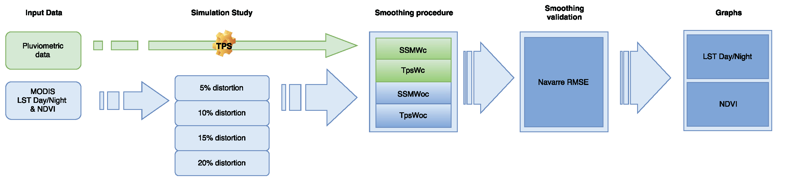
Figure 2.
Map of Navarre region, located in the north of Spain and with a common border to the south of France. Black dots correspond to the rain gauge stations used in this study.
Figure 2.
Map of Navarre region, located in the north of Spain and with a common border to the south of France. Black dots correspond to the rain gauge stations used in this study.

Figure 3.
From the top to bottom, boxplots of day LST (in Celsius), night LST (in Celsius), (in Celsius) and (in percentages) for the 46 time periods of 2011.
Figure 3.
From the top to bottom, boxplots of day LST (in Celsius), night LST (in Celsius), (in Celsius) and (in percentages) for the 46 time periods of 2011.
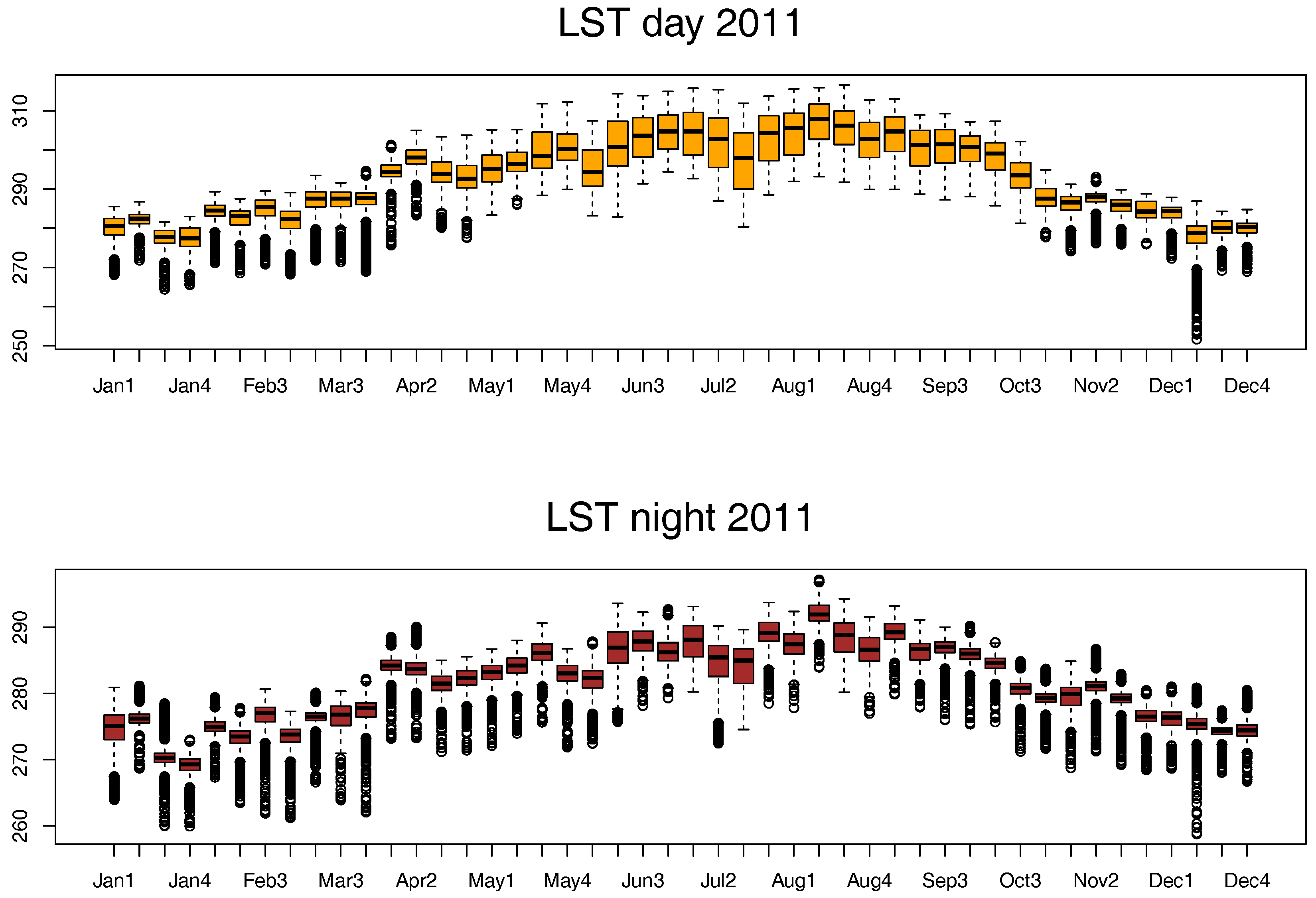

Figure 4.
Boxplots of NDVI (with a zero to 10,000 scale) in the 24 time periods of 2011.

Figure 5.
Images of Navarre for the third week of February 2014. At the top, day LST and images (in Celsius) are presented, and at the bottom, night LST (in Celsius) and (in percentages) are shown. These images show similar patterns. Black dots represent rain gauge stations.
Figure 5.
Images of Navarre for the third week of February 2014. At the top, day LST and images (in Celsius) are presented, and at the bottom, night LST (in Celsius) and (in percentages) are shown. These images show similar patterns. Black dots represent rain gauge stations.
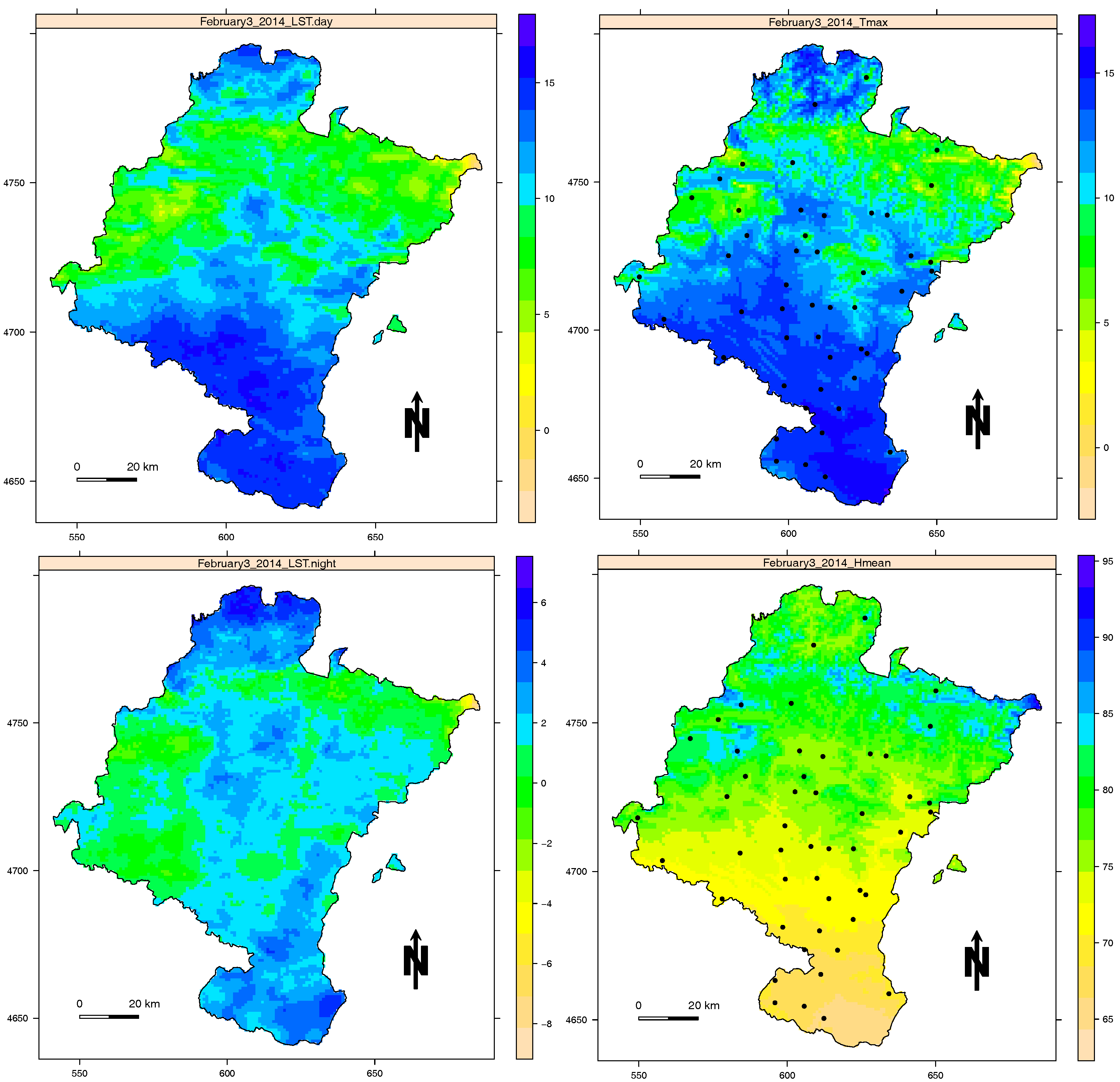
Figure 6.
On the left is the altitude map, and on the right is the NDVI image of Navarre on the second fortnight of February 2014. Both figures show similar patterns because they are highly correlated.
Figure 6.
On the left is the altitude map, and on the right is the NDVI image of Navarre on the second fortnight of February 2014. Both figures show similar patterns because they are highly correlated.
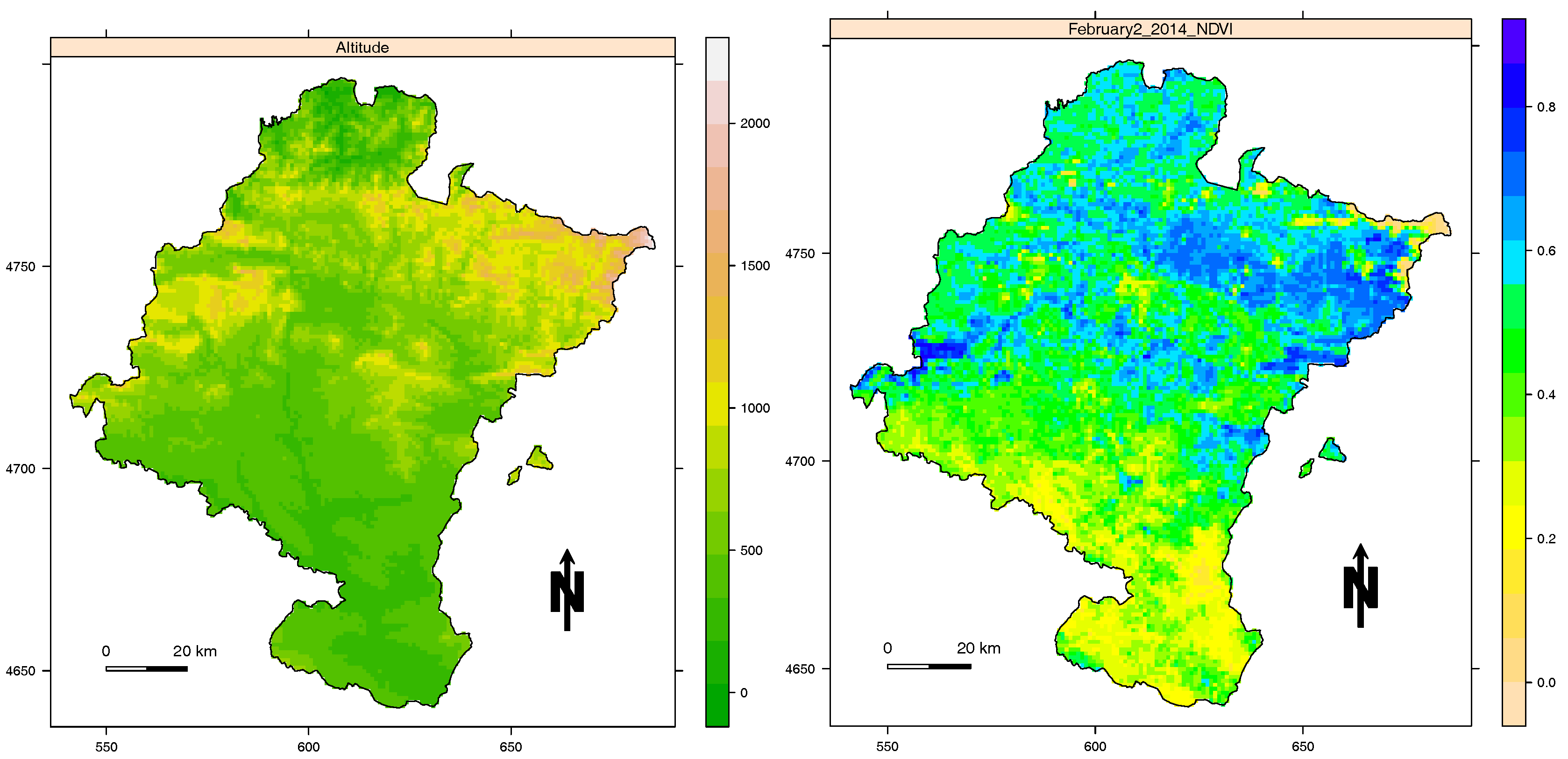
Figure 7.
Root mean square prediction error versus outlier outbreak percentage obtained for day (on the top) and night (at the bottom). Land surface temperature (LST) by climatological seasons with the four models: space-state model (SSM) with and without covariates (SSWc in red and SSMWoc in green) and Tps with and without covariates (TpsWc in blue and TpsWoc in purple).

Figure 8.
Root mean square error versus outlier outbreak percentage obtained for the normalized difference vegetation index (NDVI) by climatological season.
Figure 8.
Root mean square error versus outlier outbreak percentage obtained for the normalized difference vegetation index (NDVI) by climatological season.

Figure 9.
LST Navarra image in the fourth week of November 2011. In the upper row and from left to right, the 5% distorted image, the thin-plate spline (TpsWc) and the state-space (SSMWc) smoothed images with covariates. In the lower row and from left to right, the 20% distorted image and their respective TpsWc and SSMWc smoothed images with covariates.
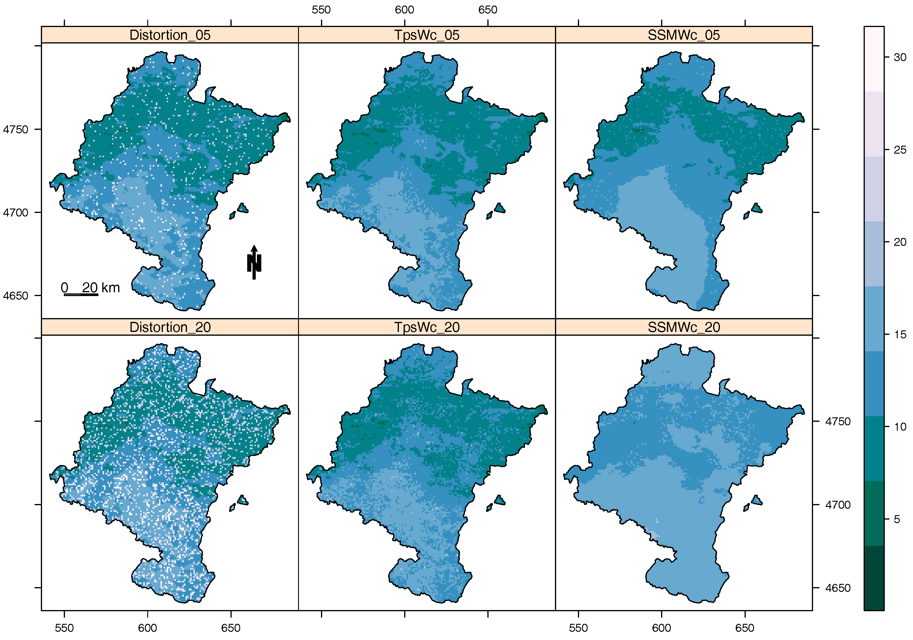
Figure 10.
At the top, boxplots of the 15% distorted images of day LST in the 46 time periods of 2011 are shown, and the bottom presents the boxplots of the smoothed day LST images by TpsWc in the same time periods.
Figure 10.
At the top, boxplots of the 15% distorted images of day LST in the 46 time periods of 2011 are shown, and the bottom presents the boxplots of the smoothed day LST images by TpsWc in the same time periods.


Table 1.
Reduction percentage of the RMSE in SSM and Tps smoothing procedures with and without covariates for day LST, night LST and NDVI for different sizes of outlier outbreaks.
Table 1.
Reduction percentage of the RMSE in SSM and Tps smoothing procedures with and without covariates for day LST, night LST and NDVI for different sizes of outlier outbreaks.
| SSM | Tps | ||||||
|---|---|---|---|---|---|---|---|
| Outlier | RMSE | RMSE | |||||
| Derived Variable | Out. % | Without Covariates | With Covariates | Reduction % | Without Covariates | With Covariates | Reduction % |
| Day | 5 | 1.80 | 1.63 | 10.19 | 0.54 | 0.51 | 7.75 |
| LST | 10 | 2.33 | 2.20 | 6.21 | 0.76 | 0.68 | 12.09 |
| 15 | 2.86 | 2.74 | 4.47 | 1.00 | 0.89 | 12.56 | |
| 20 | 3.54 | 3.44 | 2.89 | 1.37 | 1.21 | 13.31 | |
| Night | 5 | 1.34 | 1.29 | 3.90 | 0.41 | 0.37 | 11.89 |
| LST | 10 | 1.91 | 1.85 | 2.83 | 0.57 | 0.48 | 19.70 |
| 15 | 2.52 | 2.47 | 1.73 | 0.78 | 0.65 | 19.94 | |
| 20 | 3.12 | 3.08 | 1.28 | 1.13 | 0.94 | 20.36 | |
| NDVI | 5 | 0.11 | 0.09 | 19.59 | 0.04 | 0.04 | 1.68 |
| 10 | 0.11 | 0.10 | 15.11 | 0.05 | 0.05 | 1.61 | |
| 15 | 0.12 | 0.11 | 12.43 | 0.05 | 0.05 | 1.31 | |
| 20 | 0.12 | 0.11 | 10.08 | 0.05 | 0.05 | 1.56 | |
© 2018 by the authors. Licensee MDPI, Basel, Switzerland. This article is an open access article distributed under the terms and conditions of the Creative Commons Attribution (CC BY) license (http://creativecommons.org/licenses/by/4.0/).
Share and Cite
MDPI and ACS Style
Militino, A.F.; Ugarte, M.D.; Pérez-Goya, U. Improving the Quality of Satellite Imagery Based on Ground-Truth Data from Rain Gauge Stations. Remote Sens. 2018, 10, 398. https://doi.org/10.3390/rs10030398
AMA Style
Militino AF, Ugarte MD, Pérez-Goya U. Improving the Quality of Satellite Imagery Based on Ground-Truth Data from Rain Gauge Stations. Remote Sensing. 2018; 10(3):398. https://doi.org/10.3390/rs10030398
Chicago/Turabian StyleMilitino, Ana F., M. Dolores Ugarte, and Unai Pérez-Goya. 2018. "Improving the Quality of Satellite Imagery Based on Ground-Truth Data from Rain Gauge Stations" Remote Sensing 10, no. 3: 398. https://doi.org/10.3390/rs10030398
Note that from the first issue of 2016, this journal uses article numbers instead of page numbers. See further details here.