Calibration of GLONASS Inter-Frequency Code Bias for PPP Ambiguity Resolution with Heterogeneous Rover Receivers

1
Institute of Urban Smart Transportation & Safety Maintenance , Shenzhen University, Shenzhen 518060, China
2
GNSS Research Center, Wuhan University, Wuhan 430079, China
*
Author to whom correspondence should be addressed.
Remote Sens. 2018, 10(3), 399; https://doi.org/10.3390/rs10030399
Submission received: 9 January 2018
/
Revised: 9 February 2018
/
Accepted: 16 February 2018
/
Published: 5 March 2018
(This article belongs to the Special Issue Multi-Constellation Global Navigation Satellite Systems: Methods and Applications)
Abstract
:Integer ambiguity resolution (IAR) is important for rapid initialization of precise point positioning (PPP). Whereas many studies have been limited to Global Positioning System (GPS) alone, there is a strong need to add Globalnaya Navigatsionnaya Sputnikovaya Sistema (GLONASS) to the PPP-IAR solution. However, the frequency-division multiplexing of GLONASS signals causes inter-frequency code bias (IFCB) in the receiving equipment. The IFCB causes GLONASS wide-lane uncalibrated phase delay (UPD) estimation with heterogeneous receiver types to fail, so GLONASS ambiguity is therefore traditionally estimated as float values in PPP. A two-step method of calibrating GLONASS IFCB is proposed in this paper, such that GLONASS PPP-IAR can be performed with heterogeneous receivers. Experimental results demonstrate that with the proposed method, GLONASS PPP ambiguity resolution can be achieved across a variety of receiver types. For kinematic PPP with mixed receiver types, the fixing percentage within 10 min is only 33.5% for GPS-only. Upon adding GLONASS, the percentage improves substantially, to 84.9%.
1. Introduction
With precise satellite orbit and clock corrections, precise point positioning (PPP) can provide decimeter- to centimeter-level kinematic positioning results directly referenced to the global reference frame. Such positioning does not require a dense reference network and has proven to be a powerful tool in a number of applications, such as those pertaining to geophysics and meteorology [1,2]. Integer carrier-phase ambiguity resolution (IAR) is important to shorten the initialization time and improve the precision of traditional PPP. In contrast to relative positioning, because only one receiver is involved in PPP, the uncalibrated phase delay (UPD) will be absorbed by the ambiguity estimates, which makes it impossible to fix the ambiguities to integers [3]. UPDs must therefore be separated from precise satellite clock products and applied in PPP to fix the ambiguities. Mervart et al. [4] proposed a phase-only method for PPP-IAR. Ge et al. [5] estimated the single-difference between-receiver wide-lane (WL) and narrow-lane (NL) frequency code biases (FCBs), achieving PPP-IAR over a global network. Later, Collins et al. [6] and Laurichesse et al. [7] used satellite clock estimates to absorb the un-differenced (UD) NL FCBs. In contrast, Bertiger et al. [8] delivered all UD ambiguity estimates that contain the FCBs to users for PPP ambiguity resolution. The traditional PPP model requires a few tens of minutes to get the first ambiguity-fixed solution [9]. In Network Real-Time Kinematic (NRTK) positioning, because atmospheric delays can be modeled precisely, rapid ambiguity resolution can be achieved. Li et al. [10] showed that if one uses precise atmospheric delays to augment PPP IAR, instantaneous PPP IAR can be also achieved. Even for Galileo and BeiDou, which do not have complete constellations, initial results of PPP-IAR have already been obtained, in [11,12]. Additionally, Liu et al. [13] showed that using GPS + BeiDou can significantly improve the fixing percentage of GPS-only PPP. Meanwhile, Globalnaya Navigatsionnaya Sputnikovaya Sistema (GLONASS), which was declared fully operational globally with 24 satellites at the end of 2011, still faces obstacles to realizing PPP-IAR, owing to its frequency-division-multiple-access signals.
Currently, the 24-satellite constellation of GLONASS uses 14 frequency channels, and only satellites at antipodal slots of an orbital plane can share the same frequency. Commonly tracked GLONASS satellites thus have slightly different frequencies, which produces both inter-frequency code bias (IFCB) and inter-frequency phase bias (IFPB) [14,15,16]. Generally, GLONASS IFPB is a linear function of frequency, which can be calibrated with the model given in [16] or estimated in real time [17]. The IFCB behaves abnormally, varying not only with receiver type but also possibly antennas, domes, and firmware. Currently, there is no general model to correct IFCB [15,18,19,20,21]. Although IFCBs have little effect on short-baseline differential ambiguity resolution [16,20,22], they totally undermine ambiguity resolution in PPP, because PPP relies on the Hatch–Melbourne–Wübbena (HMW) combination [23,24,25] of code and carrier phase observations to resolve WL ambiguity. The presence of IFCB results in a biased WL ambiguity estimation, thereby causing PPP ambiguity resolution to fail.
Liu et al. [26] used a network of homogeneous receivers to perform GLONASS UPD estimation and PPP-IAR, obtaining a preliminary result for GLONASS-only static PPP. Banville [27] formed an ionosphere-free combination with wavelength ~5 cm for GLONASS PPP ambiguity resolution. However, very limited improvements were achieved in shortening the initialization time for kinematic PPP-IAR, owing to the relatively short wavelength. Reussner and Wanninger [15] proposed the use of a precise ionospheric model to directly fix WL ambiguity with the WL combination of L1 and L2 carrier-phase observations. However, this method depends on a precise ionospheric delay model (precise enough to fix the WL ambiguity with a wavelength of ~86 cm), which devalues its application. Geng and Bock [28] adopted this idea and found that 92.4% of all fractional parts of GLONASS WL ambiguities agreed well within ±0.15 cycles, but the efficiency of PPP-IAR for GLONASS is lower than that for the GPS; only 63% of hourly solutions were fixed for GLONASS while 97% were fixed for the GPS. Geng and Shi [29] used a regional network of receivers with mutual separation 300 km to calculate ionospheric corrections to aid this method. Results showed that the GPS + GLONASS fixing percentage with observation length 10 min could be improved to 87.50%. Yi et al. [30] calibrated the odd cycle in the HMW combination to achieve GLONASS PPP-IAR, showing that the positioning accuracy of GPS + GLONASS PPP could be improved substantially after ambiguity fixing. Liu et al. [31] compared WL phase-combination-based GLONASS PPP-IAR with HMW-combination-based GLONASS PPP-IAR, proposing that the HMW-based method is independent of the ionosphere model and therefore far superior to the latter over large areas, where one cannot obtain a precise ionosphere model.
According to the reviews in the previous paragraphs, it is still a challenge to resolve the GLONASS PPP ambiguity with heterogeneous receivers. In the present study, we propose a method for calibrating GLONASS P1/P2 IFCBs to achieve PPP-IAR using the HMW method over heterogeneous rover receivers. The proposed method is validated first with the same dataset of homogeneous receivers used by Liu et al. [31] as a reference, to check its efficiency. We then use a network of mixed receivers in France to examine their efficiency over heterogeneous receivers. The remainder of the paper is organized as follows. We first describe the method for UPD estimation at the server. We then introduce the proposed method for GLONASS IFCB estimation in detail. We use a network of homogeneous receivers and a network of heterogeneous receivers to validate the method. Finally, discussion and concluding remarks are presented based on our findings.
2. Methods
After correcting the IFPB with a linear model [16], the code and phase observations of frequency can be written as
where and denote a satellite and receiver respectively, and and are code and carrier phase observations with corresponding wavelength and frequency . is the nondispersive delay that includes geometric delay, tropospheric delay, satellite and receiver clock biases, and any other delay that affects all observations identically. The quotient denotes the slant ionospheric delay, the integer ambiguity, and the code IFB. Finally, and denote un-modeled code and carrier phase errors including multipath effects and noise. The phase center correction and phase windup effect [32] must be considered in modeling. To eliminate the first-order ionosphere delay, the well-known ionospheric-free (IF) combination is usually used for PPP [2]:
where ; and . The related float ionosphere-free ambiguity is usually expressed as the combination of WL and NL integer ambiguities and their UPDs:
where and are the integer WL and NL ambiguities, respectively, with corresponding wavelengths and . and are the receiver and satellite NL UPDs, respectively.
2.1. GLONASS UPD Estimation Strategy
The NL code and WL carrier phase observation can be defined as
where is the NL IFCB (in meters) and is the WL ambiguity with corresponding wavelength . Thus, we obtain the WL ambiguity as
with
where and are the receiver and satellite WL UPDs, respectively. is the receiver WL IFCB (in cycles).
According to Equation (6), the existence of the receiver-and-satellite-dependent WL IFCB will undermine the WL UPD estimation [15,26]. If we use receivers with identical IFCBs, the WL IFCB for a particular satellite will be the same for all involved receivers and can be absorbed into the satellite UPD estimates. Equation (5) can thus be rewritten as
where . With this reformulation, we have eliminated the effect of the receiver WL IFCB, and GLONASS PPP ambiguity fixing can therefore be carried out in a straightforward manner. According to Equations (3) and (7), GLONASS un-differenced WL and NL UPDs can be generated with the strategy proposed in [7].
2.2. Rover IFCB Correction Method
Equation (7) shows that the estimated WL UPD contains the IFCB of the reference stations, and is thus only be suitable for receivers with the same IFCB. Otherwise, we must correct the IFCB difference with respect to the reference stations. As a result of the ionosphere delay, we propose the two-step correction method described in the following.
2.2.1. Correcting the Large Part
Given a receiver to be calibrated, we can select the nearest reference station to ensure the largest number of commonly observed satellites. We can then write the between-station-differenced NL code observation and the IF code and carrier phase observation equations as
where represents the single difference between stations. and denote the NL and IF IFCB difference with respect to the reference station. In the first and second equations of (8), the IFCB parameters strongly depend on the corresponding receiver clocks, so we add a zero-mean constraint on all NL and IF IFCB estimates.
We obtain the NL and IF IFCB corrections by daily static baseline processing using (8). Since we have used homogeneous receivers as the reference stations, one can select three or more surrounding reference stations to estimate the IFCB and use average values. With the NL and IF IFCB estimates, we can attain the P1 and P2 IFCB corrections:
Because of the residual ionosphere delays that have not been eliminated, the estimated IFCB correction is biased and it is not possible to fix the WL ambiguities. We thus need to further refine the IFCB estimates.
2.2.2. Correcting the Fractional Part
We first process daily static PPP using the WL and NL UPD products generated from the reference stations. The estimated WL and NL ambiguities have been corrected with the satellite UPD products. The P1 and P2 IFCB corrections have also been applied to the code observations. Therefore, considering the IFCB residuals, the WL ambiguity can be expressed as
where represents the residual WL IFCB. Not that, the integer part is not separable from the integer ambiguity, thus we only have to further estimate the fractional part of the residual WL IFCB.
Assuming that m GLONASS satellites can be observed and there are two continuous tracking arcs for each satellite, and we have fixed all WL ambiguities in Equation (10), we then get
where and represent the float WL ambiguities for the two arcs of satellite m, and and are for the fixed integers. Given Equation (11), the WL IFCB residuals can be estimated in a least-squares manner. The WL ambiguity fixing procedure is described as follows.
- (a)
- Select the ambiguity with the longest tracking arc, assume the WL IFCB residual is zero for the satellite, and fix the WL and NL ambiguities by rounding. The receiver UPD can thus be separated from all WL and NL float ambiguities.
- (b)
- Select another WL and NL ambiguity pair. First round down the WL ambiguity and if the corresponding NL ambiguity can be fixed, fix the WL ambiguity as the rounded-down value. If not, round up the WL ambiguity and if the corresponding NL ambiguity can be fixed, fix the WL ambiguity as the rounded-up value.
- (c)
- Repeat (b) for all remaining WL and NL ambiguity pairs.
After obtaining the accurate fractional part of the WL IFCB correction, we can get the NL IFCB correction with (6), which can be used to correct the initial value obtained via (8) and get the final P1 and P2 IFCB estimates using (9). Although we only estimate the fractional part of the residual WL IFCB, Equation (9) reveals that the P1 and P2 IFCB estimates both satisfy the WL ambiguity resolution and the high-precision of IF code observation. Thus, the proposed IFCB calibration method will not be affected by the ionospheric residuals, so we do not need a dense reference network.
3. Data and Processing Strategy
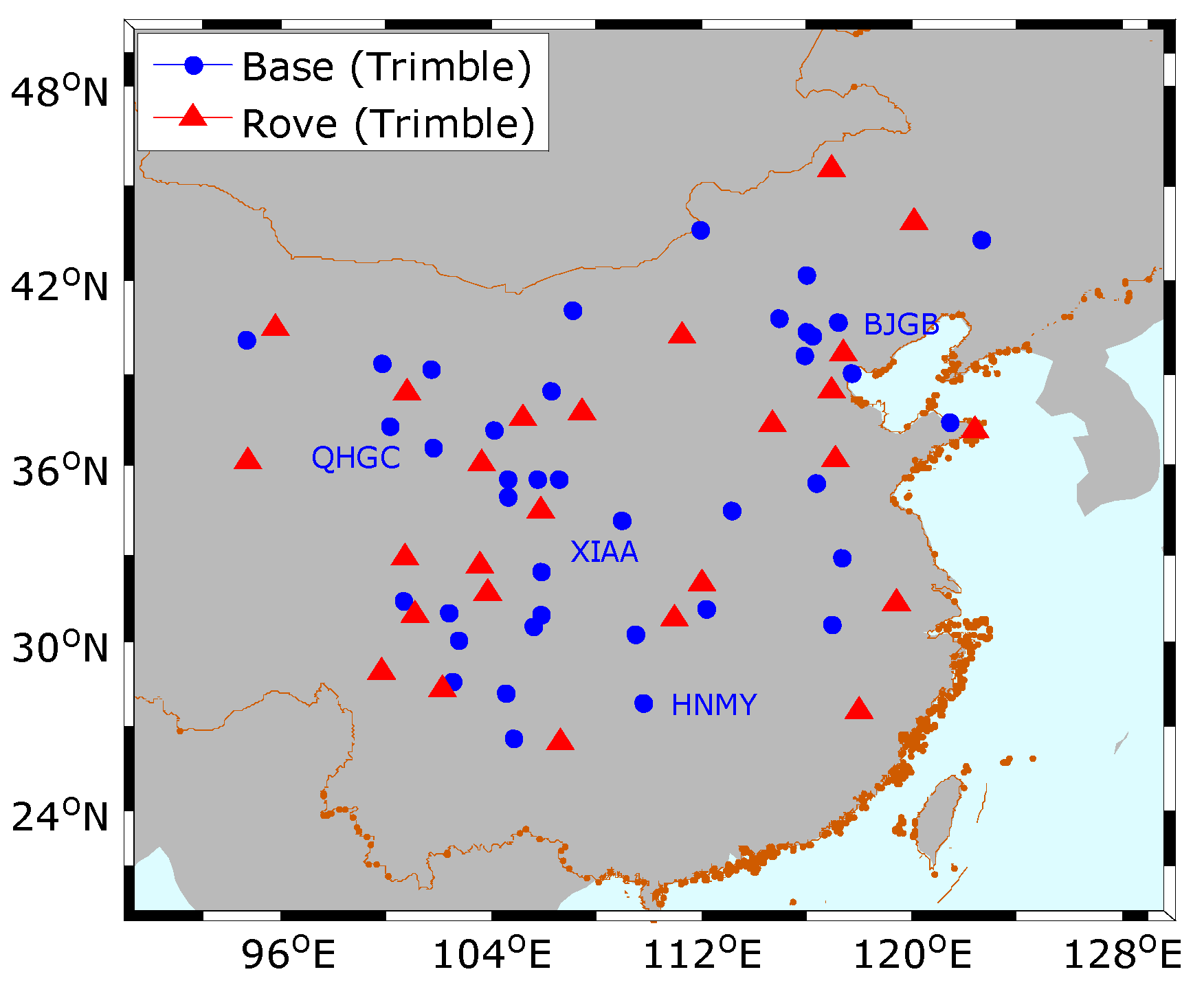
We first assessed the proposed method using 66 stations with identical hardware configurations from the Crustal Movement Observation Network of China [26]. All these stations are equipped with the same receiver (Trimble NetR8, Sunnyvale, California, USA) and antenna (TRM59800.00 SCIS, Sunnyvale, California, USA) types. Therefore, after neglecting the unit variations, we can assume that these receivers have comparable code IFB, and GLONASS PPP-IAR can thus be performed without considering IFCB corrections. This allows a control-group experiment to assess the proposed IFCB estimation strategy. Three weeks (covering days of year (DOY) 1–21 in 2013) of data collected at sampling interval 30 s were processed. 26 stations were used as base stations to generate the UPD products and the remaining 40 stations were used as rover stations to perform PPP-IAR. Figure 1 shows the distribution of these stations.
We also selected 18 base stations with the same hardware configuration to generate UPDs, and 28 rover stations with diverse hardware configurations to assess the performance of the proposed method. Both the base and rover stations are located in France. All base stations are equipped with Trimble NetR5 receivers, whereas the rover stations have Trimble, Leica and TPS receivers plus a variety of antennas, domes, and firmware versions. Detailed information about the base and rover stations is given in Table 1. The distribution of the stations is shown in Figure 2. Data covering DOY 1–21 in 2013 with sampling interval 30 s were processed.
The proposed strategy was implemented in Positioning and Navigation Data Analyst (PANDA) software [33], developed at Wuhan University, to process GPS + GLONASS data. The absolute phase center correction, phase wind-up effects, and station displacement models proposed by IERS conventions 2003 were applied. The a priori tropospheric zenith delays were calculated with the Saastamoinen model [34] and mapped into the slant ones with the global mapping function [35]. Eclipsing GPS and GLONASS satellites were deleted to avoid the effect of poorly modeled satellite attitudes. The final GPS/GLONASS orbit and clock products from the European Space Agency/European Space Operations Centre IGS analysis center [36] were fixed in both the UPD estimation and PPP-IAR.
A priori precisions of 1 and 0.01 m were used for the IF code and carrier phase observations respectively. A cutoff angle of 7° was set for the GPS and GLONASS, and an elevation-dependent weighting strategy was used to weight measurements. Owing to inter-system bias, we estimated the individual receiver clock for GPS and GLONASS. The common zenith tropospheric delay was estimated as a piecewise constant every 60 min. We used C1 and P2 code observations for GLONASS for the reference network, whereas for the rover receivers either C1 or P1 can be used with P2 observations.
We divided the daily observations into 24 pieces of hourly sets, and PPP-IAR was performed using a simulated kinematic model for each hourly dataset. Daily static PPP-IAR was first performed for each rover station to attain the “true” ambiguity, which could be used to assess the correctness of hourly PPP-IAR in the kinematic model. The LAMBDA method was used to search for integer NL ambiguity, and the ratio test used to validate ambiguity resolution with a threshold of 2 [31]. The initial fixing time in each hourly session was recorded and analyzed. We further calculated the cumulative distribution of the initial fixing time, obtaining the fixing rate for different observation durations. To fully assess the effectiveness of the proposed method for different receiver types, we analyzed the fixing percentage as a function of the conducted stations. Since we used only one day of data to generate the IFCB corrections, to analyze its effectiveness, we also analyzed the fixing percentage on each of the 21 days.
4. Results and Validation
In this section, we first assess the proposed method with the first network of homogeneous receivers. The other network of heterogeneous receivers is then used to further validate the method.
4.1. Assessment of Homogeneous Receivers
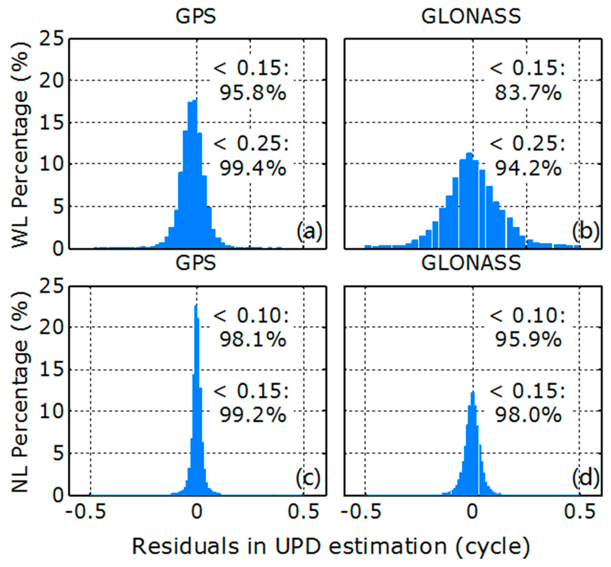
We first check the quality of the WL and NL UPD products, which are critical for PPP ambiguity resolution. This can be done by examining the a posteriori residuals of the float WL and NL ambiguities. Figure 3 shows a statistical histogram of these residuals. The figure shows that for the WL ambiguity, 95.8% of residuals are within 0.15 cycles of the nearest integer for the GPS, whereas only 83.7% are within 0.15 cycles for GLONASS. However, 94.2% of GLONASS WL residuals are within 0.25 cycles, which satisfies the WL ambiguity resolution. For the NL ambiguity, more than 95% of residuals are within 0.1 cycles for GPS and GLONASS, and more than 98% are within 0.15 cycles for both. The proposed WL IFCB calibration method only relies on the NL UPD, which has the same high quality as that of the GPS, so the lower quality of GLONASS WL UPD will not affect the proposed IFCB calibration method.
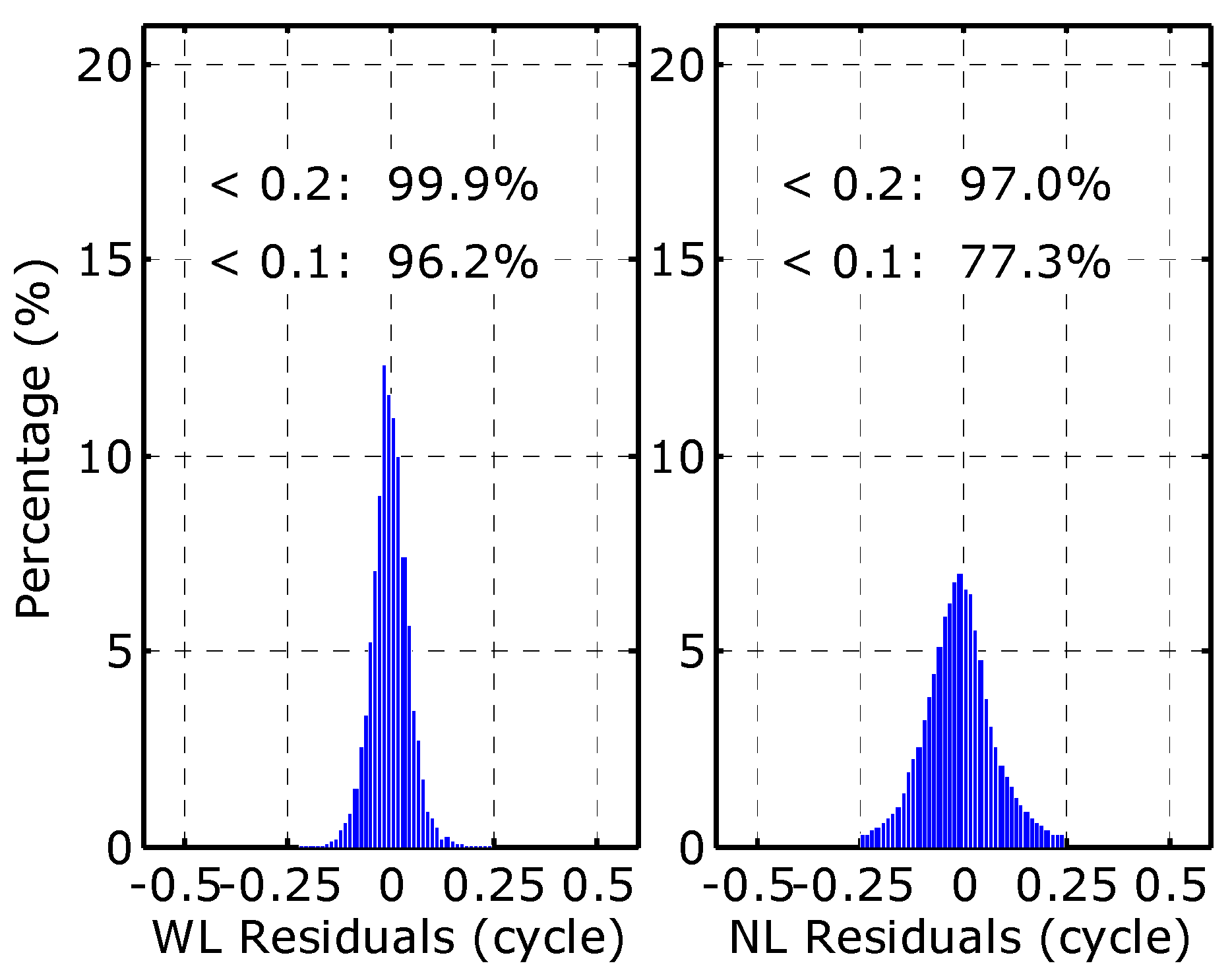
The quality of the IFCB estimates can be checked by examining residuals of the WL and NL ambiguities in the estimation. Figure 4 shows a statistical histogram of these residuals. For some satellites, there is only one ambiguity and the WL residual is thus zero; we deleted the WL residuals for these satellites. The figure shows that for the NL ambiguity, 77.3% of residuals are within 0.1 cycles and 97.0% are within 0.2 cycles, which means that 97.0% of all GLONASS ambiguities were used for WL IFCB estimation. For the WL ambiguity, 96.2% and 99.9% of residuals are within 0.1 and 0.2 cycles, respectively. The WL residuals are smaller than the NL residuals because of the much longer WL wavelengths (~0.84 m). These statistics confirm that the IFCB estimates are of good quality.
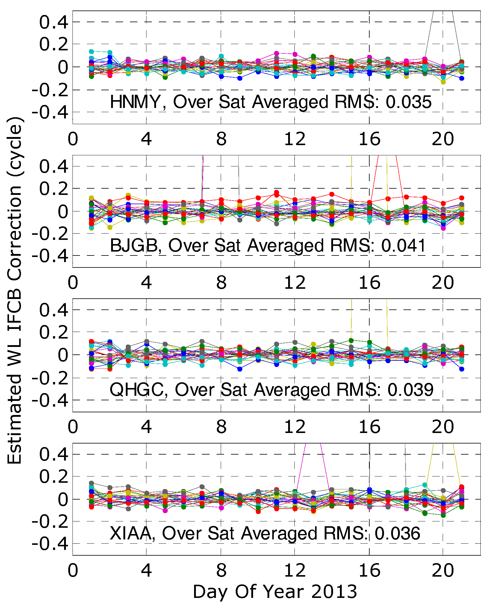
To assess the stability of IFCB estimates, we selected four representative stations distributed evenly across the network. Figure 5 portrays time series of their WL IFCB estimates because they are critical for WL ambiguity fixing. It is seen that estimates of the WL IFCB are relatively stable, and values for different days agree with each other to better than 0.05 cycles (root-mean-square or RMS value). The IFCB can, therefore, be calibrated at update intervals of several days or even longer. Thus, in the following analysis, the IFCB estimates on the first day were used for PPP-IAR.
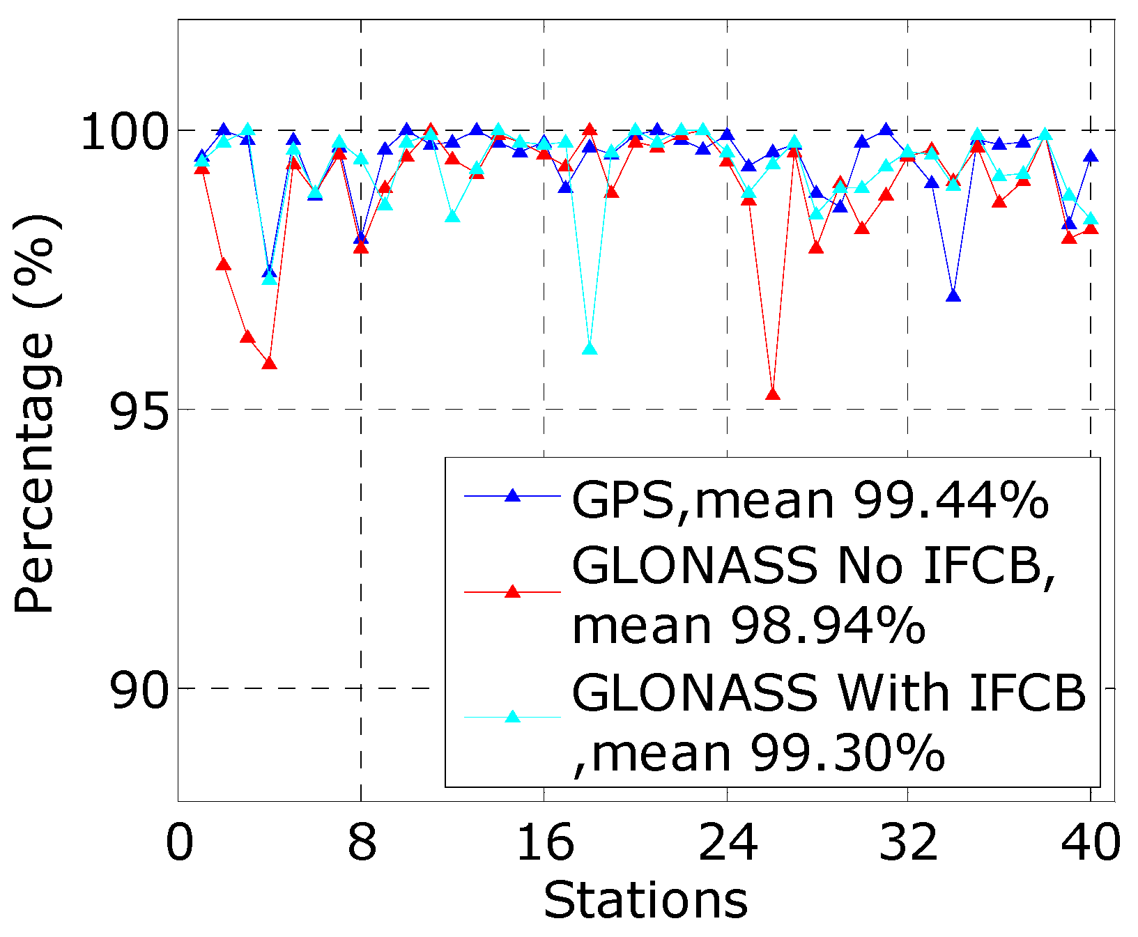
To further validate the quality of the IFCB corrections, we processed GPS + GLONASS daily static PPP-IAR for each rover station. We attempted to fix ambiguities with a tracking arc longer than 30 min by rounding with the criterion of 0.2 cycles. Figure 6 shows the average daily fixing percentage for each station. For all stations, the fixing percentage is over 97.1% and 95.3% for the GPS and GLONASS, respectively, with averages 99.4% and 98.9%. Upon applying the IFCB corrections, the average fixing percentage for GLONASS improves to 99.3%. For GLONASS, 32 stations show improvement. Among the degraded stations, two stations have degradations of 3.9% and 1.0%, whereas the others have degradation within 0.4%.
To comprehensively analyze the efficiency of the IFCB calibration method, we performed kinematic PPP-IAR for all hourly observations of the 40 rover stations using three models, i.e., GPS-only PPP, combined GPS + GLONASS PPP without IFCB calibration, and combined GPS + GLONASS PPP with IFCB calibration.
We first calculated the IFCB corrections using data of 3 days, and compared improvement in fixing percentage with respect to the one-day IFCB corrections. Results are shown in Figure 7. The figure shows that for an observation time shorter than 10 min, the fixing percentage improves almost equally using either one-day IFCB or three-day IFCB corrections. For an observation time longer than 25 min, improvement in the one-day IFCB is within −0.007 to −0.004% while that in the three-day IFCB within −0.002 to 0.001%. The improvement in fixing percentage achieved using three-day IFCB corrections is thus very little, less than 0.005%. Therefore, we propose that one-day IFCB estimates may be adequate for GLONASS PPP-IAR, although multi-day data would allow more reliable IFCB estimates.
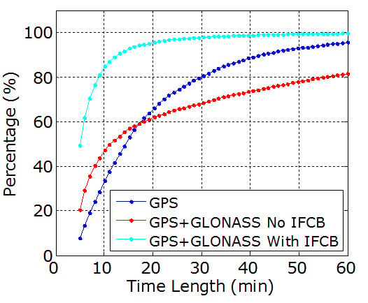
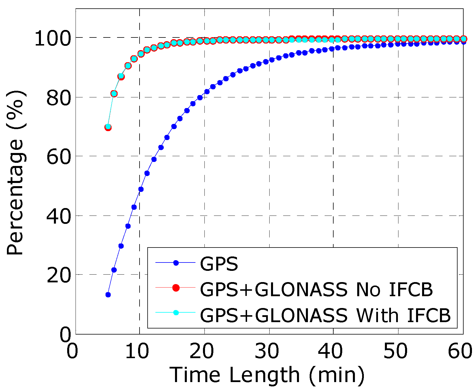
We performed simulated kinematic PPP-IAR for all the hourly datasets of the 40 rover stations, and got the fixing percentage as a function of observation duration, which is shown in Figure 8; while Table 2 gives typical values for observation durations 5, 10 and 15 min. It is seen that upon adding GLONASS, the fixing percentage for the GPS-only solution can be improved for different observation durations. By further applying IFCB calibration, the fixing percentage barely improves, i.e., the improvement is only 0.28% and 0.01% for observation durations 5 and 10 min, respectively. The small improvements mean that the IFCBs are slightly different even in the receivers with the same type. For observation duration of 15 min, the fixing percentage even degrades, by 0.04%. This might be because IFCB estimates obtained using only one day of data are not perfect, but the effect on the fixing percentage is so small that it may be neglected.
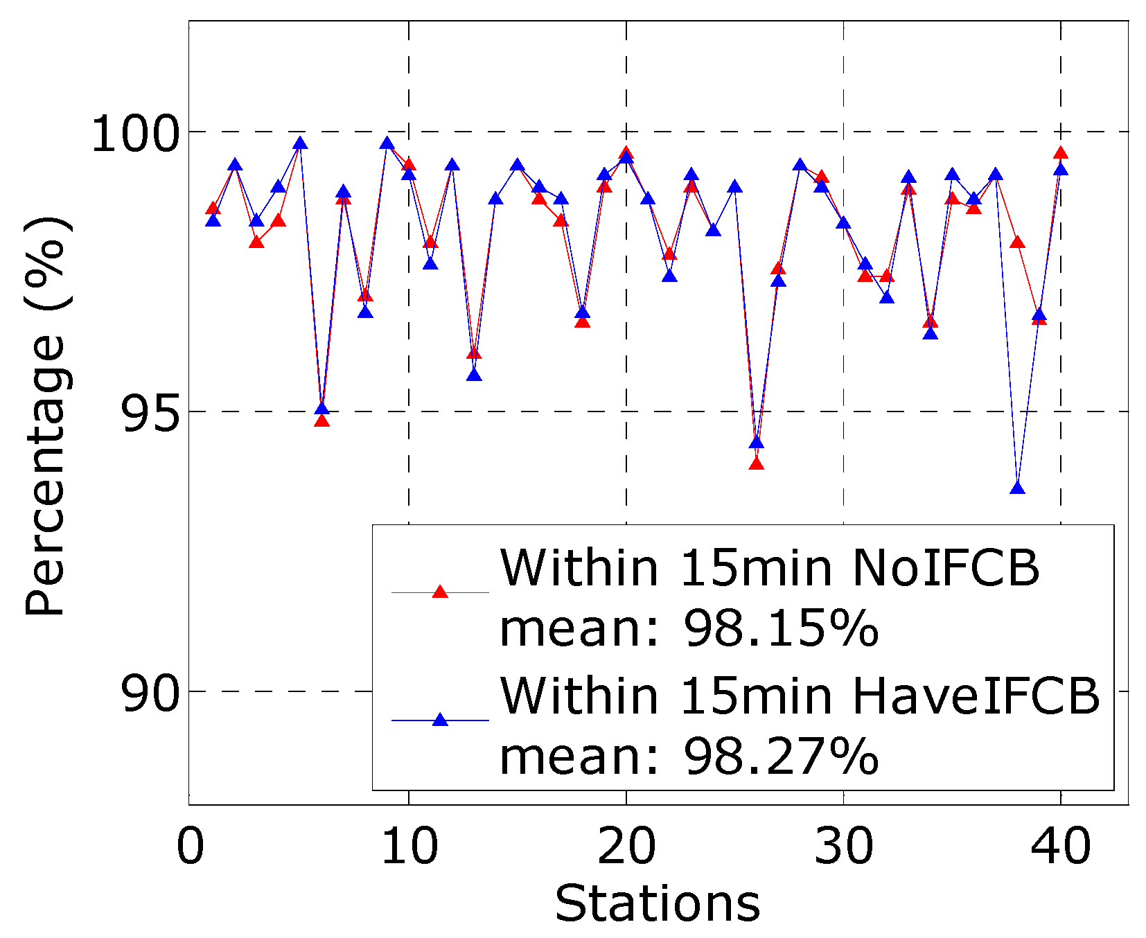
Figure 9 shows the fixing percentage for GPS + GLONASS kinematic PPP, with and without IFCB calibration, for observation duration of 15 min for each station. Among the 40 rover stations, 13 show little degradation upon applying the IFCB corrections. The degraded fixing percentages are within 0.39% except for the 38th station, for which it was 4.3%. For all remaining 27 stations, the improvements in fixing percentages by IFCB corrections are below 0.59%. The over-station average fixing percentage improves from 98.15 to 98.27%.
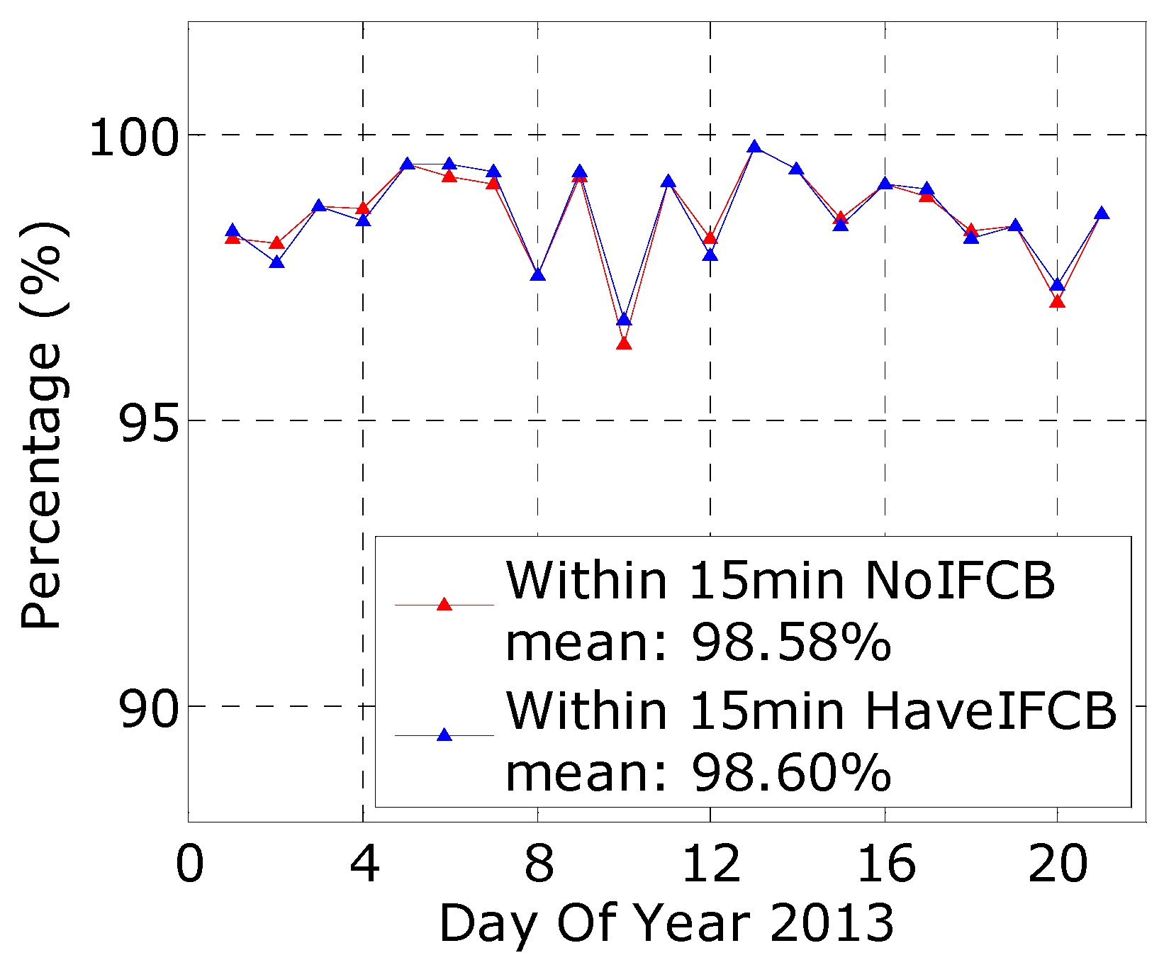
We also calculated the fixing percentage for GPS + GLONASS kinematic PPP, with and without IFCB calibration, for observation duration of 15 min on each day (Figure 10). The figure shows that among the 21 days, the fixing percentages are degraded on 5 days but the maximum degradation was within 0.31%. For the remaining 16 days, the fixing percentages improve but by less than 0.43%. The over-day-averaged fixing percentage improves from 98.58 to 98.60%.
These statistics reflect two findings. First, the IFCB of selected rover stations agrees well with that of the base stations used to calculate the WL and NL UPDs. Second, the proposed method can even achieve better performance than the homogeneous receivers.
4.2. Assessment of Heterogeneous Receivers
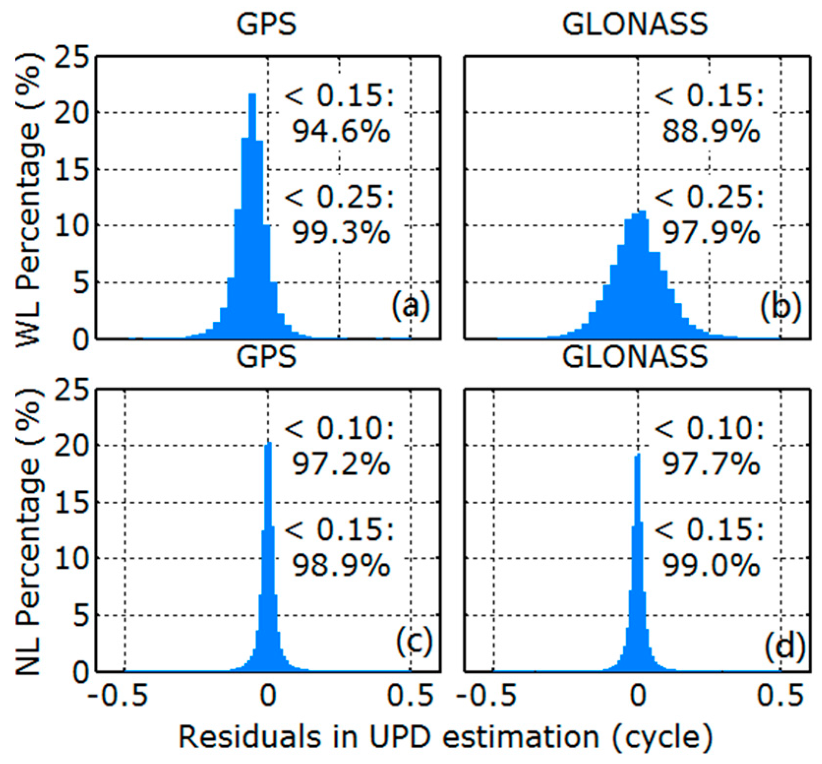
We first performed UPD estimation using the 18 base stations in the second network. The quality of the UPD products was first checked by examining the a posteriori residuals of the float WL and NL ambiguities, the statistical histogram for which is shown in Figure 11. For the WL ambiguity, 94.6% of GPS residuals are within 0.15 cycles, whereas only 88.9% of GLONASS residuals are within 0.15 cycles. However, 97.9% of GLONASS WL residuals are within 0.25 cycles. For the NL residuals, more than 97% and 98% are within 0.1 and 0.15 cycles for GPS and GLONASS, respectively. The UPD products, therefore, have the same quality as those calculated using Trimble NetR8 receivers.
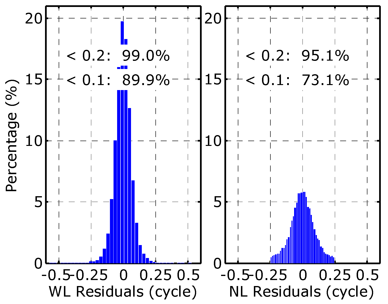
Figure 12 shows a histogram of the residuals of the WL and NL ambiguities in the WL IFCB estimation. We deleted the WL residuals for satellites that have only one arc. The figure shows that 73.1% of the NL residuals are within 0.1 cycles, while and 95.1% within 0.2 cycles. For the WL ambiguity, 89.9% and 99.0% of residuals are within 0.1 and 0.2 cycles, respectively. These statistics reveal that the proposed IFCB calibration method works well for heterogeneous receiver types.
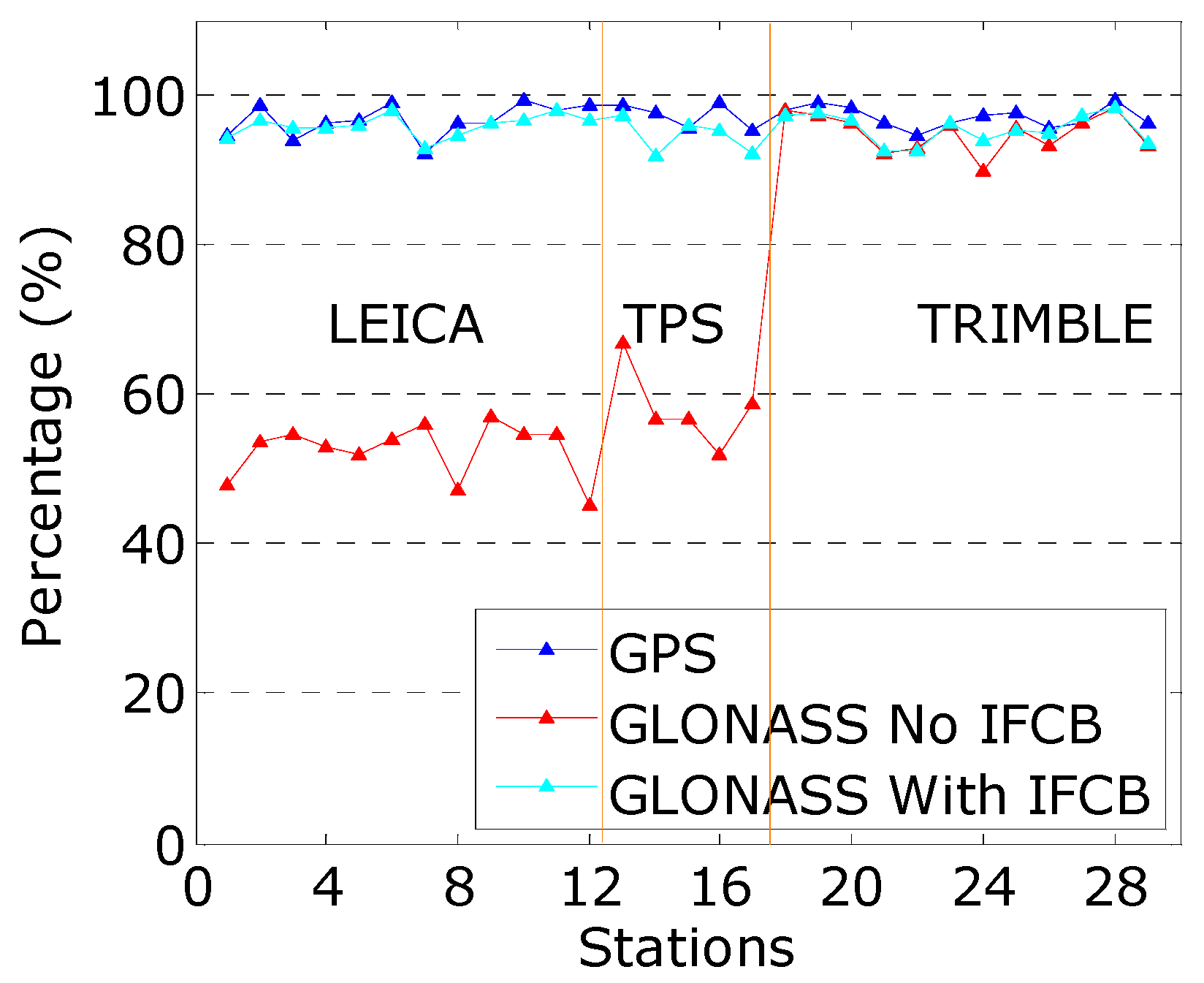
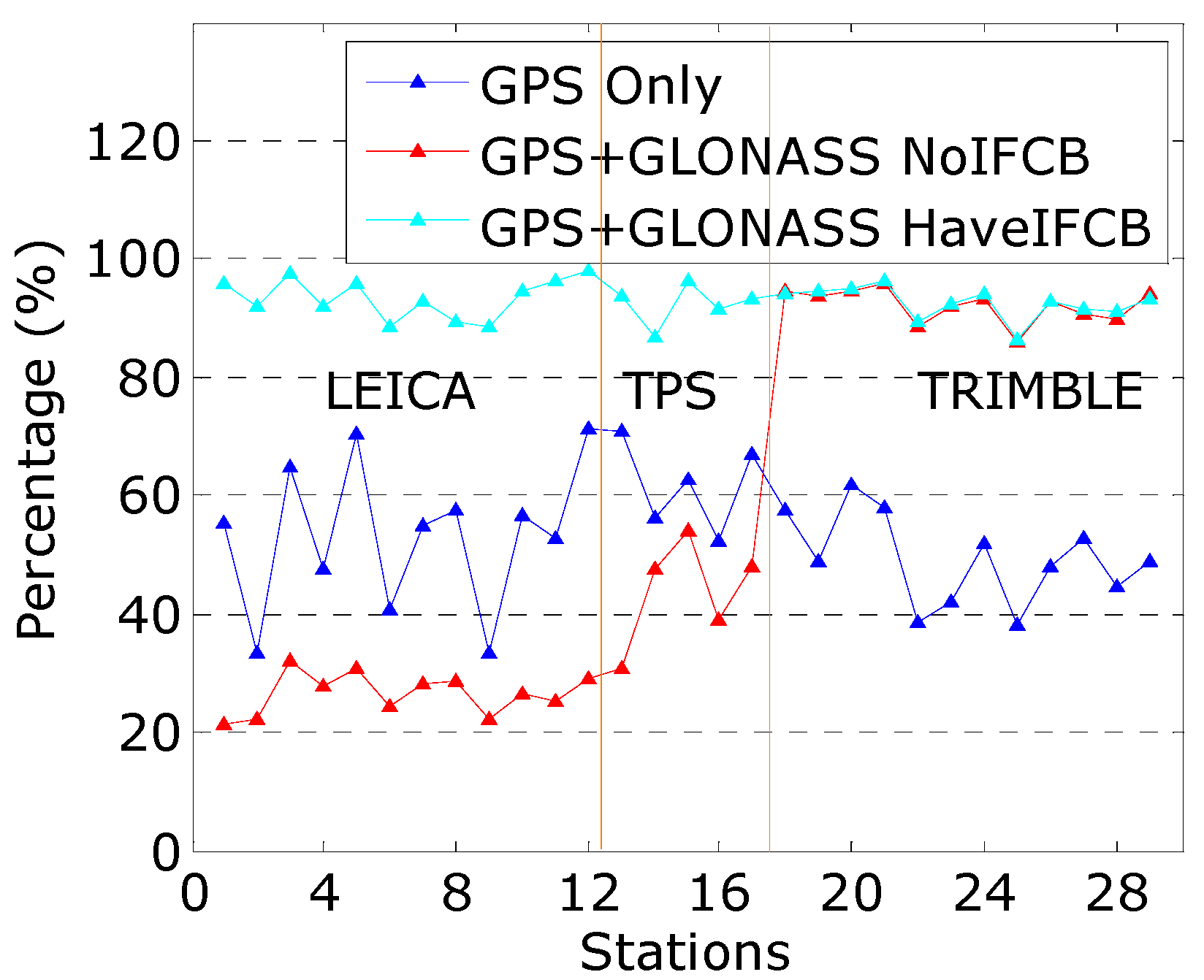
To validate the quality of the IFCB corrections, we processed GPS + GLONASS daily static PPP-IAR for each rover station. The processing strategy is the same as that shown in Figure 5. The average daily fixing percentage for each station is shown in Figure 13, and the over-manufacturer-averaged daily fixing percentage is summarized in Table 3. The fixing percentages of the GPS exceed 92.2% for all stations and average 96.6%, 97.3% and 97.1% for Leica, TPS, and Trimble receivers, respectively. For GLONASS without IFCB corrections, the fixing percentage is below 66% for the 17 Leica and TPS receivers, and over 89.9% for the 12 Trimble receivers. Upon applying the IFCB corrections, they exceed 91.9% for all 29 receivers and average 95.9%, 94.5% and 95.5% for Leica, TPS, and Trimble receivers.
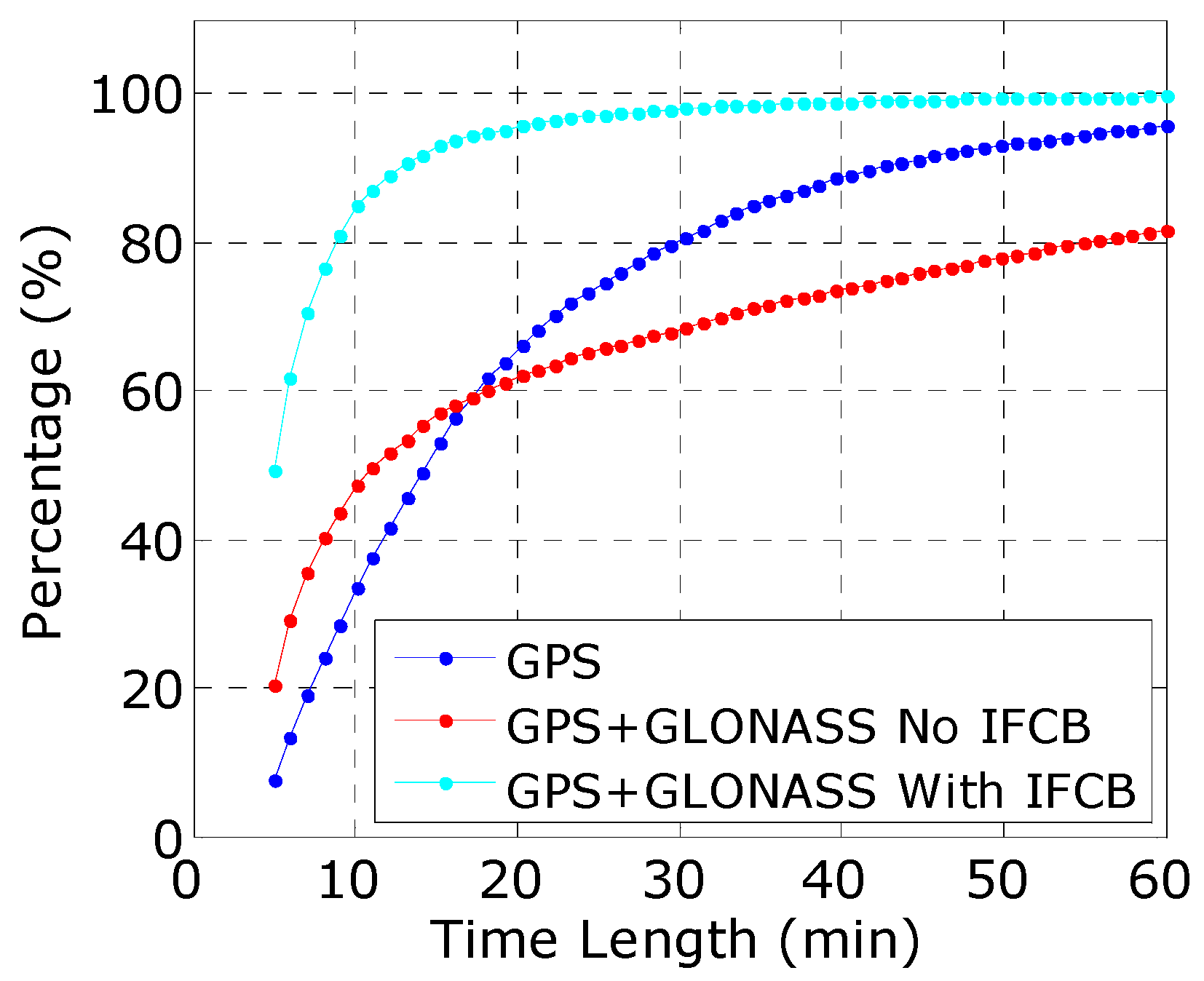
Kinematic precise point positioning-integer ambiguity resolution (PPP-IAR) was also performed for all hourly datasets of the 29 rover stations using the three models. The fixing percentage of all hourly solutions for different observation durations was calculated and is shown in Figure 14, and typical values for observation durations of 5, 10 and 15 min are given in Table 4. The fixing percentages for GPS-only for observation durations 5, 10 and 15 min are very small. Upon adding GLONASS without considering IFCB corrections, the fixing percentages are even lower than that of the GPS-only solution when the observation durations exceeded 17 min. The fixing percentage improves significantly by considering IFCB corrections.
The fixing percentage in Figure 14 is smaller than that in Figure 8. We believe this may be attributed to the data quality in the network being lower than that corresponding to Figure 7. This can be inferred by two findings. First, the fixing percentage of GPS-only for observation durations 5, 10 and 15 min is lower than that obtained from the first network, by 5.8%, 15.5%, and 17.1%, respectively. Second, a comparison of Figure 6 and Figure 13 shows that the fixing percentage of static PPP is lower than that for the first network. To further validate our speculation, we applied kinematic PPP-IAR to the 18 base stations and calculated the fixing percentage as shown in Figure 15. Since there is no “base station” to calculate the P1 and P2 IFCBs, we only calculated WL IFCB for the base stations. It is seen that the fixing percentage for the base stations is similar to that calculated using the rover stations. The difference is within 3%, 1.3% and 1% for observation durations 5, 10 and 15 min, respectively. It is thus confirmed that the smaller fixing percentage in Figure 14 is from the poorer data quality of the network and not a problem with the method.
To present the improvement achieved upon applying IFCB corrections for each receiver type, Figure 16 shows the fixing percentage of kinematic PPP for different processing strategies for observation duration of 15 min for each station. The over-manufacturer-average fixing percentage is summarized in Table 5. The figure shows that the fixing percentage for GPS-only is below 71% for each station. For GPS + GLONASS without IFCB corrections, the fixing percentage is 30% for the 12 Leica receivers and below 55% for the five TPS receivers; all values are smaller than the corresponding GPS-only solutions. Upon applying the IFCB corrections, the fixing percentage for GPS + GLONASS improves to over 88% for these 17 stations. For the 12 Trimble stations, because they have an IFCB similar to that of the base stations, the improvement was not appreciable upon applying the IFCB corrections; all improvements are below 1.2% and there is even small degradation for two stations (0.2% and 0.6%).
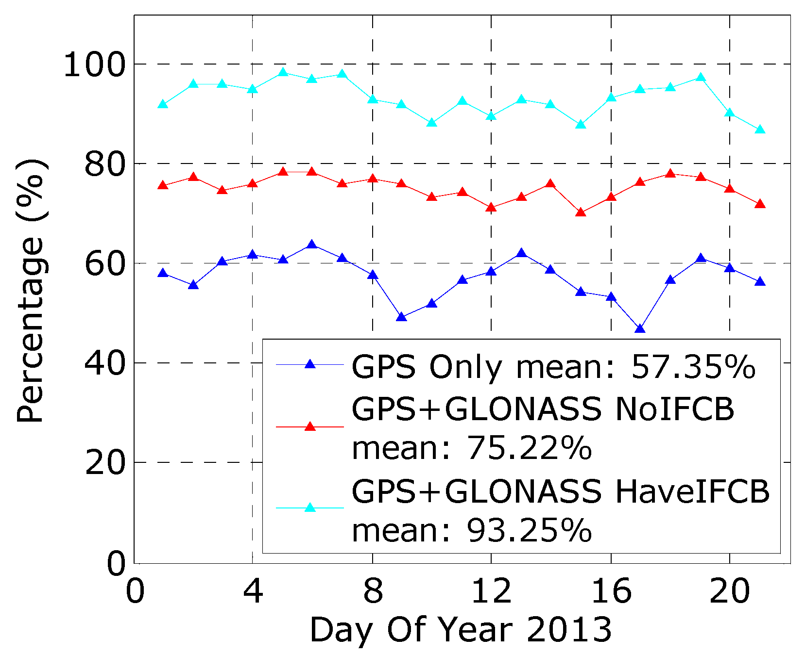
The fixing percentage for kinematic PPP using different processing strategies for observation duration of 15 min on each day is shown in Figure 17. The fixing percentage is between 47% and 63% on each day for GPS-only and between 70.2% and 78.5% for GPS + GLONASS without IFCB corrections. Upon applying IFCB corrections, the fixing percentages exceed 86.9% for all days and average 93.3%.
We calculated the position RMS of each fixed epoch, and the results are shown in Table 6. For GPS + GLONASS PPP, because the ambiguity fixing percentage is very small without IFCB correction, we only calculated the RMS with IFCB calibration. On average, the position RMS is 0.80, 0.68 and 2.79 cm for GPS-only in the north, east and up directions, respectively, whereas it degrades to 0.66, 0.60 and 2.45 cm for GPS + GLONASS, with improvements of 17.5%, 11.8% and 12.1%.
The above results confirm that the proposed IFCB calibration method is efficient for GPS + GLONASS PPP-IAR with heterogeneous receivers.
5. Discussion
Although there have been several published studies on the topic of GLONASS PPP ambiguity resolution, the problem caused by the IFCB in WL ambiguity fixing has not been well resolved. The shortcomings in the current studies are: they require homogeneous receivers for both UPD estimation and PPP-IAR [26,31]; or require a very high-precise ionosphere model [15,29]; or use an extra-narrow-lane combination with a short wavelength of only about 5 cm [27]. It’s revealed by Liu et al. [31] that, we should use the HMW method for GLONASS PPP-IAR, because it is independent on the precise ionosphere model and has a relatively long wavelength. In this study, we proposed a strategy for calibrating the GLONASS IFCB to achieve rapid GPS + GLONASS PPP-IAR with heterogeneous receivers over a large area. Experiment results show that the proposed IFCB calibration method is efficient for heterogeneous receivers and can even achieve better performance than the homogeneous receivers.
The presented method is limited in its application to existing networks, in that it requires a reference network of homogeneous receivers. However, rapid PPP ambiguity fixing is only required in industrial applications provided by commercial companies, who tend to establish their own reference network rather than rely on existing global navigation satellite system networks with few homogeneous receivers. For example, both Trimble (Sunnyvale, California, USA) and Fugro (Leidschendam, The Netherlands) have their own reference network of homogeneous receivers [37,38]. Furthermore, because the proposed IFCB calibration method does not rely on a dense reference network of homogeneous receivers, it is easy for commercial companies to deploy a sparse network of homogeneous receivers at intervals 500–1000 km to provide a GPS + GLONASS rapid PPP ambiguity fixing service in an area.
6. Conclusions
Using multi-GNSS can substantially improve the fixing percentage of PPP-IAR. GLONASS is the second worldwide positioning system, and the use of GPS + GLONASS will contribute greatly to the performance of PPP-IAR. However, IFCB prevents GLONASS ambiguity fixing with heterogeneous receivers. This paper proposes a method of calibrating GLONASS IFCB, such that PPP-IAR can be performed across heterogeneous rover receivers. This will make it possible to provide commercial real-time PPP service with rapid ambiguity resolution using multi-GNSS constellations.
We first assessed the efficiency of the method with 21-day data collected by a network of 66 Trimble NetR8 receivers. As homogeneous receivers are used for both UPD estimation and PPP-IAR, PPP-IAR can be performed without considering the IFCB effect and can be used to assess the performance of the IFCB calibration method. The results show that we need only one day of data to estimate the IFCB, and the estimated daily IFCB for different days is consistent for better than 0.05 cycles (RMS). Upon adding GLONASS without IFCB correction, the fixing percentage within 5 min improves from 13.23 to 69.94%. We then further applied the IFCB calibration and found that the percentage can even be slightly improved by 0.28%.
We then used a network of 29 heterogeneous rover receivers to validate the method and the data collection also extended over 21 days. Before applying the IFCB calibration, the fixing percentage for GPS + GLONASS is even smaller than the GPS-only solution. Upon applying the IFCB calibration, the fixing percentage improves for receivers from each manufacturer. The average fixing percentage within 15 min for the 12 Leica, 5 TPS, and 12 Trimble receivers is 93.4%, 92.3%, and 92.6%, respectively. These values are comparable to results for reference stations of homogeneous receivers. Upon adding GLONASS, the positioning accuracy of ambiguity-fixed PPP solutions improves by 17.5%, 11.8%, and 12.1% for the north, east, and upward directions. These results confirm that the proposed IFCB calibration method is efficient for GPS + GLONASS PPP-IAR with heterogeneous rover receivers.
Acknowledgments
We thank the Crustal Movement Observation Network of China (CMONOC), IGN and ESA for providing the observation data and precise products. This work was partially supported by the National Key Research and Development Program of China (Nos. 2016YFB0800405, 2016YFB0502203, 2016YFB0501802), National Natural Science Foundation of China (Nos. 41704033, 41074008, 41504028, 41374034, 41404010, 41301511, 41604028, 41604017, 41401444), National 973 Program of China (No. 2012CB957701), and Shenzhen future industry development funding program (No. 201507211219247860).
Author Contributions
Yanyan Liu conceptualized the initial idea and experimental design. Shengfeng Gu performed the experiments and wrote the main manuscript text. Qingquan Li helped with data collection and results analysis.
Conflicts of Interest
The authors declare no conflict of interest.
References
- Kouba, J.; Héroux, P. Precise point positioning using IGS orbit and clock products. GPS Solut. 2001, 5, 12–28. [Google Scholar] [CrossRef]
- Zumberge, J.; Heflin, M.; Jefferson, D.; Watkins, M.; Webb, F. Precise point positioning for the efficient and robust analysis of GPS data from large networks. J. Geophys. Res. 1997, 102, 5005–5017. [Google Scholar] [CrossRef]
- Gabor, M.J.; Nerem, R.S. GPS carrier phase AR using satellite-satellite single difference. In Proceedings of the ION GNSS-1999, Nashville, TN, USA, 14–17 September 1999; pp. 1569–1578. [Google Scholar]
- Mervart, L.; Lukes, Z.; Rocken, C.; Iwabuchi, T. Precise Point Positioning with ambiguity resolution in real-time. In Proceedings of the ION GNSS-2008, Savannah, GA, USA, 16–19 September 2008; pp. 397–405. [Google Scholar]
- Ge, M.; Gendt, G.; Rothacher, M.; Shi, C.; Liu, J. Resolution of GPS carrier phase ambiguities in precise point positioning (PPP) with daily observations. J. Geodesy 2008, 82, 389–399. [Google Scholar] [CrossRef]
- Collins, P.; Lahaye, F.; Héroux, P.; Bisnath, S. Precise point positioning with AR using the decoupled clock model. In Proceedings of the ION GNSS-2008, Savannah, GA, USA, 16–19 September 2008; pp. 1315–1322. [Google Scholar]
- Laurichesse, D.; Mercier, F.; Berthias, J.P.; Broca, P.; Cerri, L. Integer ambiguity resolution on undifferenced GPS phase measurements and its application to PPP and satellite precise orbit determination. Navigation 2009, 56, 135–149. [Google Scholar] [CrossRef]
- Bertiger, W.; Desai, S.D.; Haines, B.; Harvey, N.; Moore, A.W.; Owen, S.; Weiss, J.P. Single receiver phase ambiguity resolution with GPS data. J. Geodesy 2010, 84, 327–337. [Google Scholar] [CrossRef]
- Geng, J.; Teferle, F.N.; Meng, X.; Dodson, A.H. Towards PPP-RTK: Ambiguity resolution in real-time precise point positioning. Adv. Space Res. 2011, 47, 1664–1673. [Google Scholar] [CrossRef]
- Li, X.; Zhang, X.; Ge, M. Regional reference network augmented precise point positioning for instantaneous ambiguity resolution. J. Geodesy 2011, 85, 151–158. [Google Scholar] [CrossRef]
- Gu, S.; Lou, Y.; Shi, C.; Liu, J. BeiDou phase bias estimation and its application in precise point positioning with triple-frequency observable. J. Geodesy 2015, 89, 979–992. [Google Scholar] [CrossRef]
- Tegedor, J.; Liu, X.; Jong, K.; Goode, M.; Øvstedal, O.; Vigen, E. Estimation of Galileo Uncalibrated Hardware Delays for Ambiguity-Fixed Precise Point Positioning. Navigation 2016, 63, 173–179. [Google Scholar] [CrossRef]
- Liu, Y.; Ye, S.; Song, W.; Lou, Y.; Chen, D. Integrating GPS and BDS to shorten the initialization time for ambiguity-fixed PPP. GPS Solut. 2016. [Google Scholar] [CrossRef]
- Felhauer, T. On the Impact of RF Front-end Group Delay Variations on GLONASS Pseudorange Accuracy. In Proceedings of the International Technical Meeting of the Satellite Division of the Institute of Navigation 1997, Tampa, FL, USA, 8–12 September 1997. [Google Scholar]
- Reussner, N.; Wanninger, L. GLONASS Inter-frequency Biases and Their Effects on RTK and PPP Carrier phase Ambiguity Resolution. In Proceedings of the ION GNSS-2011, Portland, Oregon, 19–23 September 2011; pp. 712–716. [Google Scholar]
- Wanninger, L. Carrier phase inter-frequency biases of GLONASS receivers. J. Geodesy 2012, 86, 139–148. [Google Scholar] [CrossRef]
- Tian, Y.; Ge, M.; Neitzel, F. Particle filter-based estimation of inter-frequency phase bias for real-time glonass integer ambiguity resolution. J. Geodesy 2015, 89, 1145–1158. [Google Scholar] [CrossRef]
- Al-Shaery, A.; Zhang, S.; Rizos, C. An enhanced calibration method of GLONASS inter-channel bias for GNSS RTK. GPS Solut. 2013, 17, 165–173. [Google Scholar] [CrossRef]
- Song, W.; Yi, W.; Lou, Y.; Shi, C.; Yao, Y.; Liu, Y.; Mao, Y.; Xiang, Y. Impact of glonass pseudorange inter-channel biases on satellite clock corrections. GPS Solut. 2014, 18, 323–333. [Google Scholar] [CrossRef]
- Kozlov, D.; Tkachenko, M.; Tochilin, A. Statistical characterization of hardware biases in GPS + GLONASS receivers. In Proceedings of the ION GNSS 2000, Institute of Navigation, Salt Lake City, UT, USA, 19–22 September 2000; pp. 817–826. [Google Scholar]
- Yamada, H.; Takasu, T.; Kubo, N.; Yasuda, A. Evaluation and calibration of receiver inter-channel biases for RTK-GPS/GLONASS. In Proceedings of the ION GNSS-2010, Portland, Oregon, 21–24 September 2010; pp. 1580–1587. [Google Scholar]
- Wang, J.; Leick, A.; Rizos, C.; Stewart, M.P. GPS and GLONASS integration: Modeling and ambiguity resolution issues. GPS Solut. 2001, 5, 55–64. [Google Scholar] [CrossRef]
- Hatch, R. The synergism of GPS code and carrier measurements. In Proceedings of the Third International Symposium on Satellite Doppler Positioning at Physical Sciences Laboratory of New Mexico State University, Las Cruces, NM, USA, 8–12 February 1982; Volume 2, pp. 1213–1231. [Google Scholar]
- Melbourne, W.G. The case for ranging in GPS-based geodetic systems. In Proceedings of the First International Symposium on Precise Positioning with the Global Positioning System, Rockville, MD, USA, 15–19 April 1985. [Google Scholar]
- Wübbena, G. Software developments for geodetic positioning with GPS using TI-4100 code and carrier measurements. In Proceedings of the First International Symposium on Precise Positioning with the Global Positioning System, Rockville, MD, USA, 15–19 April 1985. [Google Scholar]
- Liu, Y.; Song, W.; Lou, Y.; Ye, S.; Zhang, R. Glonass phase bias estimation and its ppp ambiguity resolution using homogeneous receivers. GPS Solut. 2016. [Google Scholar] [CrossRef]
- Banville, S. GLONASS ionosphere-free ambiguity resolution for precise point positioning. J. Geodesy 2016, 90, 1–10. [Google Scholar] [CrossRef]
- Geng, J.; Bock, Y. GLONASS fractional-cycle bias estimation across inhomogeneous receivers for PPP ambiguity resolution. J. Geodesy 2016, 90, 379–396. [Google Scholar] [CrossRef]
- Geng, J.; Shi, C. Rapid initialization of real-time PPP by resolving undifferenced GPS and GLONASS ambiguities simultaneously. J. Geodesy 2017, 91, 1–14. [Google Scholar] [CrossRef]
- Yi, W.; Song, W.; Lou, Y.; Shi, C.; Yao, Y. A method of undifferenced ambiguity resolution for GPS + GLONASS precise point positioning. Sci. Rep. 2016, 6, 26334. [Google Scholar] [CrossRef] [PubMed]
- Liu, Y.; Ye, S.; Song, W.; Lou, Y.; Gu, S.; Li, Q. Rapid PPP Ambiguity Resolution Using GPS + GLONASS Observations. J. Geodesy 2016. [Google Scholar] [CrossRef]
- Wu, J.; Wu, S.; Hajj, G.; Bertiger, W.; Lichten, S. Effects of antenna orientation on GPS carrier phase. Manuscr. Geod. 1993, 18, 91–98. [Google Scholar]
- Liu, J.; Ge, M. PANDA software and its preliminary result of positioning and orbit determination. Wuhan Univ. J. Nat. Sci. 2003, 8, 603–609. [Google Scholar]
- Saastamoinen, J. Contributions to the theory of atmospheric refraction. Bull. Géodésique 1972, 105, 279–298. [Google Scholar] [CrossRef]
- Boehm, J.; Niell, A.; Tregoning, P.; Schuh, H. Global mapping function (GMF): A new empirical mapping function based on numerical weather model data. Geophys. Res. Lett. 2006, 33, L07304. [Google Scholar] [CrossRef]
- Loyer, S.; Perosanz, F.; Mercier, F.; Capdeville, H.; Soudarin, L. CNES-CLS IGS Analysis Centre products: Evaluation and recent improvements. In Proceedings of the AGU Fall Meeting. AGU Fall Meeting Abstracts, San Francisco, CA, USA, 14–18 December 2009. [Google Scholar]
- Landau, H.; Brandl, M.; Chen, X.; Drescher, R.; Glocker, M.; Nardo, A.; Nitschke, M.; Salazar, D.; Weinbach, U.; Zhang, F. Towards the inclusion of Galileo and BeiDou/Compass satellites in Trimble CenterPoint RTX. In Proceedings of the 26th International Technical Meeting of the Satellite Division of the Institute of Navigation (ION GNSS+ 2013), Nashville, TN, USA, 16–20 September 2013; pp. 1215–1223. [Google Scholar]
- Geng, T.; Xie, X.; Zhao, Q.; Liu, X.; Liu, J. Improving BDS integer ambiguity resolution using satellite-induced code bias correction for precise orbit determination. GPS Solut. 2017, 21, 1191–1201. [Google Scholar] [CrossRef]
Figure 1.
Distribution of homogeneous stations used in China.

Figure 2.
Distribution of 18 base stations and 29 rover stations used in France.
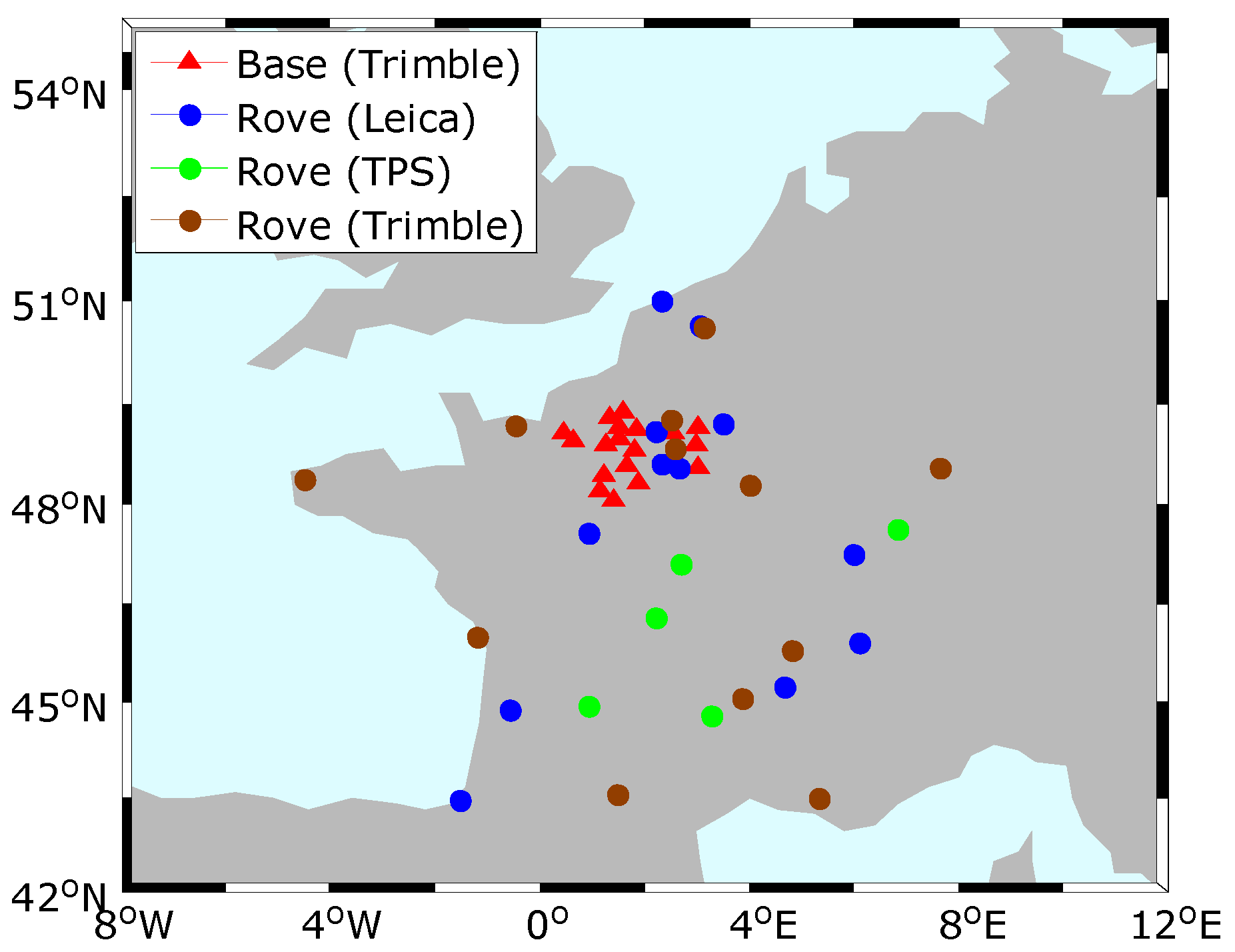
Figure 3.
Distribution of a posteriori residuals of the wide-lane (WL) (a,b) and narrow-lane (NL) (c,d) float ambiguities for Global Positioning System (GPS) and Globalnaya Navigatsionnaya Sputnikovaya Sistema (GLONASS) ((a,c) to (b,d)) in uncalibrated phase delay (UPD) estimation with reference stations.

Figure 4.
Distribution of a posteriori residuals of the WL and NL float ambiguities when performing GLONASS WL inter-frequency code bias (IFCB) calibration. Receivers with homogeneous type are used as rover sites.
Figure 4.
Distribution of a posteriori residuals of the WL and NL float ambiguities when performing GLONASS WL inter-frequency code bias (IFCB) calibration. Receivers with homogeneous type are used as rover sites.

Figure 5.
Stability of daily WL IFCB estimates of all 24 GLONASS satellites for four representative stations. Different color represents different satellites. Outliers correspond to there being no IFCB estimate for this satellite on this day.
Figure 5.
Stability of daily WL IFCB estimates of all 24 GLONASS satellites for four representative stations. Different color represents different satellites. Outliers correspond to there being no IFCB estimate for this satellite on this day.

Figure 6.
Fixing percentage of daily static precise point positioning (PPP) with different strategies for each rover station. Receivers with homogeneous type are used as rover sites.
Figure 6.
Fixing percentage of daily static precise point positioning (PPP) with different strategies for each rover station. Receivers with homogeneous type are used as rover sites.

Figure 7.
Improvement in fixing percentage for various observation durations using one-day and three-day IFCB estimates.
Figure 7.
Improvement in fixing percentage for various observation durations using one-day and three-day IFCB estimates.
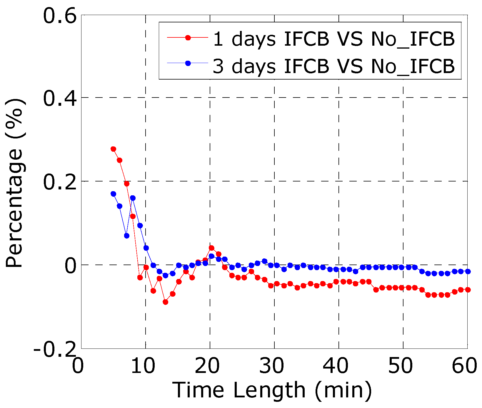
Figure 8.
Fixing percentage with various observation durations for kinematic PPP with different strategies. Receivers with homogeneous type are used as rover sites.
Figure 8.
Fixing percentage with various observation durations for kinematic PPP with different strategies. Receivers with homogeneous type are used as rover sites.

Figure 9.
Fixing percentage of kinematic PPP with different strategies for an observation duration of 15 min for each station. Receivers with homogeneous type are used as rover sites.
Figure 9.
Fixing percentage of kinematic PPP with different strategies for an observation duration of 15 min for each station. Receivers with homogeneous type are used as rover sites.

Figure 10.
Fixing percentage for kinematic PPP with different strategies for an observation duration of 15 min on each day. Receivers with homogeneous type are used as rover sites.
Figure 10.
Fixing percentage for kinematic PPP with different strategies for an observation duration of 15 min on each day. Receivers with homogeneous type are used as rover sites.

Figure 11.
Distribution of a posteriori residuals of WL (a,b) and NL (c,d) float ambiguities for GPS and GLONASS ((a,c) to (b,d)) in UPD estimation using reference stations.
Figure 11.
Distribution of a posteriori residuals of WL (a,b) and NL (c,d) float ambiguities for GPS and GLONASS ((a,c) to (b,d)) in UPD estimation using reference stations.

Figure 12.
Distribution of a posteriori residuals of WL and NL float ambiguities in GLONASS WL IFCB calibration. Receivers with heterogeneous types are used rover sites.
Figure 12.
Distribution of a posteriori residuals of WL and NL float ambiguities in GLONASS WL IFCB calibration. Receivers with heterogeneous types are used rover sites.

Figure 13.
Fixing percentage of daily static PPP with various strategies for each rover station. Receivers with heterogeneous types are used rover sites, which are grouped according to the manufacturer.
Figure 13.
Fixing percentage of daily static PPP with various strategies for each rover station. Receivers with heterogeneous types are used rover sites, which are grouped according to the manufacturer.

Figure 14.
Fixing percentage for various observation durations for kinematic PPP with different strategies. Receivers with heterogeneous types are used rover sites.
Figure 14.
Fixing percentage for various observation durations for kinematic PPP with different strategies. Receivers with heterogeneous types are used rover sites.

Figure 15.
Fixing percentage for various observation durations for kinematic PPP with different strategies for base station.
Figure 15.
Fixing percentage for various observation durations for kinematic PPP with different strategies for base station.
Figure 16.
Fixing percentage for kinematic PPP with various strategies for observation duration 15 min for each station; rover stations are grouped according to the manufacturer.
Figure 16.
Fixing percentage for kinematic PPP with various strategies for observation duration 15 min for each station; rover stations are grouped according to the manufacturer.

Figure 17.
Fixing percentage for kinematic PPP with different strategies for observation duration 15 min on each day.
Figure 17.
Fixing percentage for kinematic PPP with different strategies for observation duration 15 min on each day.


Table 1.
Detailed information about hardware configuration for 18 base stations and 29 rover stations.
Table 1.
Detailed information about hardware configuration for 18 base stations and 29 rover stations.
| Manufacturer | Receiver | Antenna | Dome | Firmware | Number | |
|---|---|---|---|---|---|---|
| Base | Trimble | NETR5 | TRM55971.00 | NONE | 4.41 | 18 |
| Rover | Trimble (Sunnyvale, California, USA) | NETR5 | TRM55971.00 | NONE | 4.19 | 1 |
| 4.48 | 3 | |||||
| 4.42 | 3 | |||||
| NETR8 | TRM55971.00 | NONE | 4.48 | 1 | ||
| NETR9 | TRM57971.00 | NONE | 4.61 | 1 | ||
| 4.60 | 2 | |||||
| TRM59800.00 | NONE | 4.60 | 1 | |||
| Leica (Heerbrugg, Switzerland) | GR10 | LEIAS10 | NONE | 1.10 | 2 | |
| 2.00/4.007 | 1 | |||||
| GRX1200 + GNSS | LEIAR25 | LEIT | 7.8 | 1 | ||
| TPSCR.G3 | TPSH | 8.51 | 1 | |||
| GRX1200GGPRO | LEIAR25 | LEIT | 7.5 | 4 | ||
| 8.51 | 1 | |||||
| LEIAT504GG | LEIS | 2.62 | 1 | |||
| GX1230GG | LEIAT504GG | LEIS | 5.10 | 1 | ||
| TPS (Tokyo, Japan) | NETG3 | TPSCR.G3 | TPSH | 4.0 | 3 | |
| 3.4 | 2 |
Table 2.
Fixing percentage with various observation durations for kinematic PPP with different strategies.
Table 2.
Fixing percentage with various observation durations for kinematic PPP with different strategies.
| Time (min) | GPS Only (%) | GPS + GLONASS | |
|---|---|---|---|
| No IFCB (%) | With IFCB (%) | ||
| 05 | 13.23 | 69.94 | 70.22 |
| 10 | 48.98 | 94.80 | 94.81 |
| 15 | 70.03 | 98.27 | 98.23 |
Table 3.
Over-manufacturer-averaged fixing percentage of daily static PPP with various strategies.
| Manufacture | GPS Only (%) | GPS + GLONASS | |
|---|---|---|---|
| No IFCB (%) | With IFCB (%) | ||
| LEICA | 96.69 | 52.52 | 95.91 |
| TPS | 97.33 | 58.11 | 94.53 |
| TRIMBLE | 97.08 | 94.97 | 95.49 |
Table 4.
Fixing percentage for various observation durations for kinematic PPP with different strategies.
Table 4.
Fixing percentage for various observation durations for kinematic PPP with different strategies.
| Time (min) | GPS Only (%) | GPS + GLONASS | |
|---|---|---|---|
| No IFCB (%) | With IFCB (%) | ||
| 05 | 7.43 | 20.41 | 49.14 |
| 10 | 33.52 | 47.14 | 84.88 |
| 15 | 52.92 | 56.92 | 92.86 |
Table 5.
Over-manufacturer-average fixing percentage with different strategies for observation duration 15 min.
Table 5.
Over-manufacturer-average fixing percentage with different strategies for observation duration 15 min.
| Manufacture | GPS Only (%) | GPS + GLONASS | |
|---|---|---|---|
| No IFCB (%) | With IFCB (%) | ||
| LEICA | 53.19 | 26.51 | 93.44 |
| TPS | 61.83 | 43.90 | 92.34 |
| TRIMBLE | 49.18 | 92.15 | 92.58 |
Table 6.
Position RMS (cm) for kinematic ambiguity fixed PPP solutions.
| Solution Type | North | East | Up |
|---|---|---|---|
| GPS Only | 0.80 | 0.68 | 2.79 |
| GPS + GLONASS With IFCB | 0.66 | 0.60 | 2.45 |
© 2018 by the authors. Licensee MDPI, Basel, Switzerland. This article is an open access article distributed under the terms and conditions of the Creative Commons Attribution (CC BY) license (http://creativecommons.org/licenses/by/4.0/).
Share and Cite
MDPI and ACS Style
Liu, Y.; Gu, S.; Li, Q. Calibration of GLONASS Inter-Frequency Code Bias for PPP Ambiguity Resolution with Heterogeneous Rover Receivers. Remote Sens. 2018, 10, 399. https://doi.org/10.3390/rs10030399
AMA Style
Liu Y, Gu S, Li Q. Calibration of GLONASS Inter-Frequency Code Bias for PPP Ambiguity Resolution with Heterogeneous Rover Receivers. Remote Sensing. 2018; 10(3):399. https://doi.org/10.3390/rs10030399
Chicago/Turabian StyleLiu, Yanyan, Shengfeng Gu, and Qingquan Li. 2018. "Calibration of GLONASS Inter-Frequency Code Bias for PPP Ambiguity Resolution with Heterogeneous Rover Receivers" Remote Sensing 10, no. 3: 399. https://doi.org/10.3390/rs10030399
Note that from the first issue of 2016, this journal uses article numbers instead of page numbers. See further details here.