Modeling Wildfire-Induced Permafrost Deformation in an Alaskan Boreal Forest Using InSAR Observations


1
Roy M. Huffington Department of Earth Sciences, Southern Methodist University, Dallas, TX 75205, USA
2
Earth Resources Observation and Science Center, United States Geological Survey, Sioux Falls, SD 57198, USA
3
United States Geological Survey, Reston, VA 20192, USA
*
Author to whom correspondence should be addressed.
Remote Sens. 2018, 10(3), 405; https://doi.org/10.3390/rs10030405
Submission received: 22 December 2017
/
Revised: 24 February 2018
/
Accepted: 2 March 2018
/
Published: 6 March 2018
(This article belongs to the Special Issue Remote Sensing of Dynamic Permafrost Regions)
Abstract
:The discontinuous permafrost zone is one of the world’s most sensitive areas to climate change. Alaskan boreal forest is underlain by discontinuous permafrost, and wildfires are one of the most influential agents negatively impacting the condition of permafrost in the arctic region. Using interferometric synthetic aperture radar (InSAR) of Advanced Land Observation Satellite (ALOS) Phased Array type L-band Synthetic Aperture Radar (PALSAR) images, we mapped extensive permafrost degradation over interior Alaskan boreal forest in Yukon Flats, induced by the 2009 Big Creek wildfire. Our analyses showed that fire-induced permafrost degradation in the second post-fire thawing season contributed up to 20 cm of ground surface subsidence. We generated post-fire deformation time series and introduced a model that exploited the deformation time series to estimate fire-induced permafrost degradation and changes in active layer thickness. The model showed a wildfire-induced increase of up to 80 cm in active layer thickness in the second post-fire year due to pore-ice permafrost thawing. The model also showed up to 15 cm of permafrost degradation due to excess-ice thawing with little or no increase in active layer thickness. The uncertainties of the estimated change in active layer thickness and the thickness of thawed excess ice permafrost are 27.77 and 1.50 cm, respectively. Our results demonstrate that InSAR-derived deformation measurements along with physics models are capable of quantifying fire-induced permafrost degradation in Alaskan boreal forests underlain by discontinuous permafrost. Our results also have illustrated that fire-induced increase of active layer thickness and excess ice thawing contributed to ground surface subsidence.
1. Introduction
Permafrost plays a significant role in landscape stability, carbon cycling, and socioeconomic development, and is key to regulating biological, hydrological, geophysical, and biogeochemical processes [1]. Roughly 37% of the Northern Hemisphere permafrost occurs in western North America, mainly in Alaska and northern Canada, but also further south in the Rocky Mountains [2]. A huge amount of carbon is stored in permafrost [3], roughly twice as large as the amount of carbon in the atmosphere [4]; therefore, disturbance of the permafrost can significantly contribute to climate change [3]. In addition, permafrost is structurally important, and its thawing has been known to cause erosion, disappearance of lakes, landslides, and ground subsidence. The active layer, defined as the top layer of ground in areas underlain by permafrost, plays a key role in land surface processes in cold regions and is subject to annual thawing and freezing and subsequent subsidence and uplift, respectively [5].
Field surveys (including surface geophysical collections), model simulations, and remote sensing observations are used to obtain regional variation of active layer thickness (ALT) [6]. ALT is usually directly measured by using a metal rod inserted into the soil to measure the depth of thawing (e.g., [7]). However, the measurement should be done at the end of the thawing season and, if possible, in stone-free soils. Surface geophysical datasets as well as ground-penetrating radar data can also be used to provide very high resolution and accurate estimates of ALT (e.g., [8]). Although ground-based ALT measurements are accurate, they provide a spatially limited sampling of a parameter that has significant spatial variability [9]. At regional scales, using empirical and statistical relationships, ALT can be modeled at coarser spatial resolution by extrapolating ground-based measurements with air temperature, ground temperature, elevation, and surface vegetation [10,11,12,13].
In contrast, remote sensing estimation of ALT usually uses Interferometric Synthetic Aperture Radar (InSAR). Measurements to estimate ALT from seasonal ground deformation [14]. In the recent years, a few attempts have been made to estimate and model ALT using InSAR this method eliminates the need to define an empirical or statistical relationship with probing data [14]. InSAR provides an all-weather, day-or-night capability to remotely sense mm–cm surface deformation with a high spatial resolution of tens of meters or better (e.g., [15,16,17,18,19]). Able to collect Synthetic Aperture Radar (SAR) images over a large-scale area, InSAR has proven very useful for deformation monitoring over permafrost in Alaska (e.g., [9,20,21,22,23,24]). Liu et al. [21] applied InSAR using ERS-1 and -2 data to monitor surface deformation near Prudhoe Bay on the Alaskan North Slope. They studied long-term permafrost-related surface subsidence and argued that the seasonal subsidence and long-term subsidence trends are due to thaw settlement of the active layer and thawing of ice-rich permafrost near the permafrost table, respectively. Liu et al. [9] estimated the 1992–2000 average ALT of the North Slope of Alaska from InSAR-derived surface subsidence by using the SAR images for thaw season only. By comparing TerraSAR-X, RADARSAT-2, and ALOS PALSAR interferometry, Short et al. [22] concluded that ALOS-PALSAR provides the most promising data for permafrost degradation monitoring. Liu et al. [23] conducted InSAR time-series analysis using ALOS-PALSAR data to detect seasonal thaw settlement in individual drained thermokarst lake basins. Liu et al. [24] demonstrated the capability of using L-band PALSAR interferograms with short perpendicular baselines to minimize the adverse effects of coherence loss, which made it possible to quantify thermokarst. Liu et al. [25] conducted InSAR time series analysis using ALOS PALSAR data to detect an increase in surface subsidence caused by Arctic tundra fire in a permafrost region of north Alaska. Iwahana [26] investigated the northern part of the Anaktuvuk River fire scar with a two-path differential InSAR technique and measured up to 6.2 cm/year post-fire subsidence within burned tundra relative to surrounding off-scar tundra using three independent InSAR pairs of ALOS PALSAR data. In addition to the use of InSAR to quantify fire-induced permafrost deformations (e.g., [26]), some researchers have recently exploited LiDAR datasets to quantify permafrost degradation. Jones et al. [27], for example, investigated the impact of the large and severe Anaktuvuk River tundra fire on potential, post-fire thermokarst development using two airborne LiDAR datasets acquired two and seven years after the fire.
Among remote sensing methods, optical methods provide the unique opportunity to map fire scar and assess its severity. Spectral analysis of optical images can facilitate fire scar and severity mapping [28,29]. Optical methods utilize the fire-induced changes in the spectral behavior of pre- and post-fire vegetation over fire scar as well as the differences between the post-fire reflective characteristics of vegetation and off-scar surrounding environment. So far, a number of indices for burned area mapping, including differenced normalized burn ratio (dNBR) [28], relativized dNBR (RdNBR), and relativized burn ratio (RBR) [29], have been developed.
The objective of this study is two-fold. First, we intend to demonstrate the capability of L-band InSAR to monitor and quantify fire-induced permafrost deformations over interior Alaskan boreal forest. Second, we introduce a model for the fire-induced post-fire permafrost deformations. To this end, we used L-band ALOS PALSAR data to map permafrost deformations over the Big Creek fire scar, Alaska, and then introduced a model to estimate wildfire-induced changes in ALT, exploiting InSAR-detected deformations in a time series over the fire scar. The InSAR-detected deformation is then used to model fire-induced permafrost deformations in boreal forest. In boreal forest, wildfire is one of the most important agents affecting permafrost. Since a huge amount of carbon is stored in permafrost, the disturbance of the permafrost can significantly contribute to global climate change. In addition, permafrost thawing has been known to cause erosion, disappearance of lakes, landslides, and ground subsidence (e.g., [6,9,12]). In a study using airborne LiDAR, Jones et al. [29] assessed fire-induced thermokarst development and concluded that in regions with ice-rich permafrost in the Arctic, the impact of tundra fires for initiating widespread thermokarst development is greater than what has been estimated to so far.
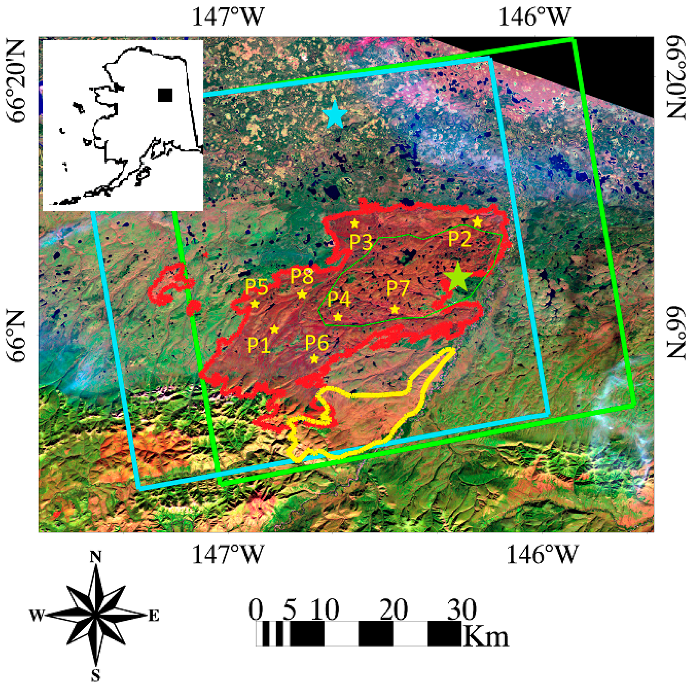
Our study area, which is underlain by discontinuous permafrost [30] and located in the Alaskan Yukon River Basin, includes the 2009 Big Creek wildfire. The fire damaged ~686 km2 from 18 July 2009, to 18 August 2009 (Figure 1). The Alaskan Yukon River Basin is mainly composed of upland and lowland evergreen forests, bottomland deciduous forest, emergent and herbaceous wetlands, upland and lowland tundra, and alpine shrub [31] and is predominantly underlain by discontinuous permafrost [30]. The near surface permafrost probability over the study area ranges from ~10% to ~70% [32]. The study area, a silty upland, was dominated by black spruce. Black spruce tends to be underlain by permafrost [33] since black spruce stands generally contain a continuous insulating layer of moss and lichens [34]. The area is in a region with low annual precipitation (about 170 mm) and particularly strong variations in seasonal temperature. In Yukon Flats, the average daily temperatures in winter and summer range from −34 °C to about −24 °C and from about 0 to about 22 °C, respectively [35].
First, we applied InSAR to measure ground surface deformations between interferometric pairs ranging from September 2009 to March 2011. Then, using the small baseline subset (SBAS) method (particularly, the TimeFun algorithm [36]), we inverted the measured InSAR phases to deformation time series. Finally, we applied our model to estimate fire-induced changes in ALT using the deformation time series. The rest of this paper is organized as follows. The InSAR analyses and results are provided in Section 2 and Section 3, respectively. In Section 4.1., we present our model and estimate wildfire-induced changes in ALT. Validation of results and estimation of uncertainties are included in Section 4.2., followed by conclusions in Section 5.
2. Methods
SAR returns must be coherent to retrieve useful information from interferograms (e.g., [37]). An InSAR coherence estimation image is a cross-correlation product of two co-registered complex-valued SAR images [37], and loss of interferometric coherence is the major obstacle for applying InSAR to monitor permafrost deformations in forested areas. InSAR coherence tends to increase with radar wavelength due to the greater capability to penetrate vegetation cover or forest canopy. For this reason, we employed L-band (23.6 cm wavelength) Japanese ALOS for InSAR analysis in the study area, which is mostly forested and underlain by permafrost. However, our inspection of InSAR coherence over the study area confirmed a strong fire-induced coherence loss that made us unable to quantify surface deformations using interferograms pairing pre- and post-fire SAR images. Figure 2 shows the ALOS coherence estimate between 17 July 2007 (pre-fire) and 06 September 2009 (post-fire) images. After the wildfire in 2009, the InSAR coherence decreased due to significant changes on the vegetation cover resulting in altered scattering characteristics from ground surface. When coherence was radically reduced to near zero values, we could not obtain useful information on the ground deformation. However, the coherence map (Figure 2) itself still can help delineate the extent of the fire scars.
Twelve HH polarized ALOS PALSAR single look complex (SLC) images, eight Fine Beam Single polarization (FBS, 28 MHz bandwidth) and four Fine Beam Dual polarization (FBD 14 MHz bandwidth), from September 2009 to March 2011 with radar look angle of 38.76° and slant range and azimuth pixel sizes of 4.68 m (in SAR coordinates) and 3.13 m, respectively, were used in this study. First, assisted by high-resolution (12 m) TanDEM-X DEM data, all SLC images have been co-registered based on a single master image, which optimizes the geometric and temporal coherence of the interferogram stack. The resampled SLC images were multi-looked by 6 and 14 in range and azimuth directions, respectively, and then used to generate initial interferograms with ground pixel sizes of about 45 m. Then, flat earth and topography phase components from initial interferograms have been removed using TanDEM-X DEM, and the interferograms were unwrapped using the Minimum Cost Flow (MCF) method [38]. Also, atmospheric correction to remove stratified tropospheric artifacts that tend to correlate with topography has been done on the interferograms by evaluating linear regression of unwrapped phase with respect to height.
The InSAR method quantifies ground surface deformation, but the geometrical and temporal decorrelations and atmospheric artifacts can affect the results. Over the last decade, a variety of SBAS algorithms have been developed and successfully applied in various ground deformation monitoring applications (e.g., [39]) aiming to generate deformation time series with artifacts removed. Generally, small baseline differential interferograms are generated first and then time series analysis is conducted (e.g., [40]). In this research, the TimeFun method, adapted from the Multiscale InSAR Time Series (MInTS) algorithm [36] and implemented in the Generic InSAR Analysis Toolbox (GIAnT) [41], was used to generate deformation time series. TimeFun adapts the same inversion strategy as that used in MInTS, but it is implemented in the data domain [36,42]. Since it uses a singular value decomposition (SVD) approach with a minimum-norm criterion, TimeFun is capable of inverting networks that are not fully connected [42]. For every pixel with a coherence value above a user-specified threshold in all interferograms, TimeFun inverts small-baseline interferometric phases into time series measurements. This method is also applied to multi-looked interferograms to further reduce decorrelation noise.
3. Results
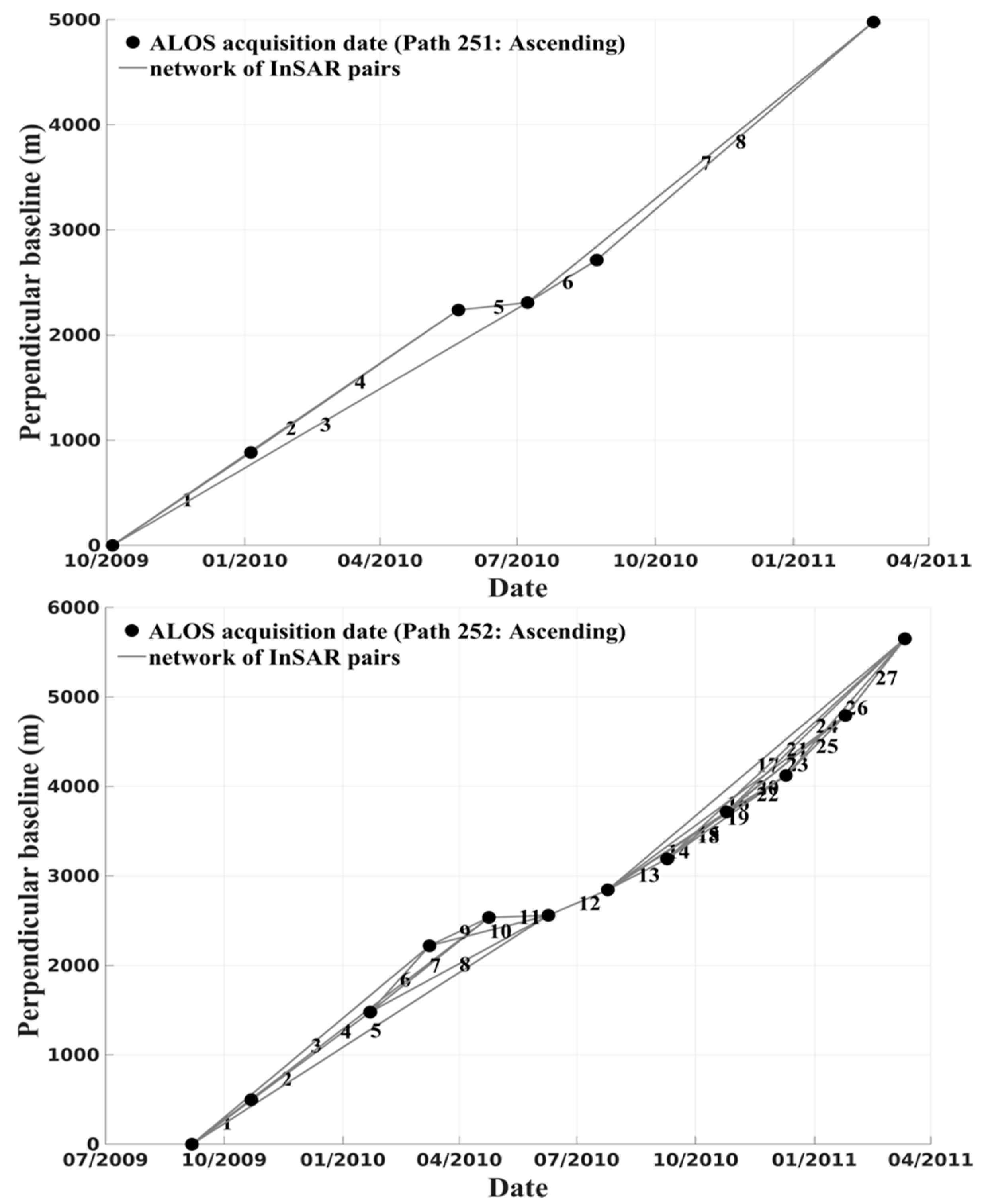
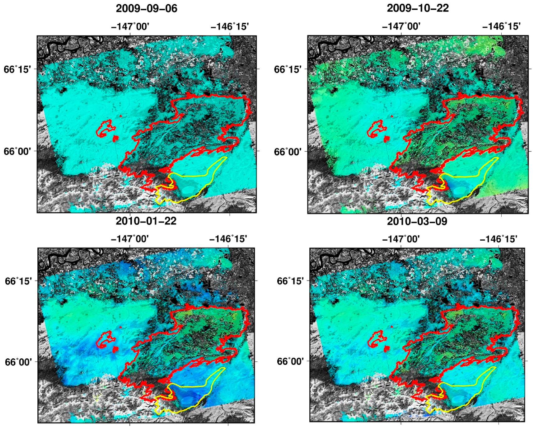
After careful inspection, 27 post-fire short baseline interferograms possessing relatively good coherence were selected to generate time series of deformations using the TimeFun method. The coherence, dependent on interferograms and ground futures, ranges from around 0.1–0.9. We used pixels with coherence values greater than 0.7 to avoid possible unwrapping errors. Permafrost process, especially post-fire surface dynamics, is complex in nature. Therefore, instead of using high order polynomials, we used spline function, i.e., piecewise polynomials, defined for example in [43], to invert the interferogram network to the time series. As permafrost thaws from top to bottom, due to the change in the type of ground ice being thawed, i.e., pore-ice and/or excess-ice permafrost, temporarily variable deformation rate can be detected by InSAR over permafrost. Regarding this complexity of post-fire deformations over permafrost, spline function seems to be a proper pre-defined function to invert the interferograms to time series deformation. However, this may make time series plots look uneven. Figure 3 shows temporal and perpendicular baselines of the interferograms. Since only one interferogram connects two clusters of the images, i.e., interferogram 12 of track 252, the quality of the time series strongly depends on it. This indicates that all noise and artifacts present in the interferogram will be propagated in the time series analysis. Moreover, because of the orbital drift of the ALOS satellite, the perpendicular baseline generally increases in time (Figure 3). Therefore, the topographic error that is proportional to the perpendicular baseline can possibly propagate in our temporal analysis. However, because our study area is flat near the Yukon River Basin, and our modeling scheme that will be presented later can cancel out the terms pertinent to the topographic errors, those errors can be assumed to be negligible. Figure 4 illustrates, from each of the tracks, two interferograms of the least connected images. The interferogram, i.e., interferogram 12 of track 252, as well as the other three interferograms illustrated in Figure 4, demonstrates expected subsidence over the fire scar. Figure 5 shows the post-fire deformation time series of path 252 where the deformations are temporarily relative to 6 September 2009, and spatially relative to a reference point (cyan star in Figure 1) that has been shown by field measurements [44] to be permafrost-free soil. As seen on the images (Figure 5), the time series demonstrates larger subsidence over the burned areas (up to 20 cm) compared to the deformation over the off-scar surrounding area (<5 cm). Generally, InSAR-detected post-fire subsidence is expected to be larger over the burned areas compared to surrounding unburned areas due to permafrost degradation and/or increased ALT as a consequence of wildfire-induced organic layer removal and soil temperature warming.
4. Discussion
Ground ice takes up about 9% more volume than groundwater in the unfrozen state. Therefore, subsidence in summer and uplift in winter occur when the active layer thaws and freezes. This repetitive pattern of ground subsidence and uplift, which can be recognized as the seasonal variations of the ground surface, is typical in most permafrost regardless of human/natural perturbations (i.e., deforestation, wildfire). Ground surface deformation over permafrost, detected by InSAR, can be closely related to the volume changes of thawing/freezing ground ice in active layer [9]. Generally, using InSAR-detected ground surface deformations, one can estimate ALT and change in ALT if the soil characteristics (porosity, saturation) in active layer are well defined.
The winter freeze and summer thaw are completely natural in a permafrost region. However, the extreme fire events in the shrub and forest-covered Alaskan region can degrade both the active layer and underlying permafrost significantly. Wildfire can be triggered by natural processes and human perturbation, but regardless of the cause of wildfires, the drastic changes on the ground surface and underground soil formations induced by high heat can lead to irreversible consequences, such as thawing of permafrost and alteration of the soil characteristics in the active layer. Because of its low coherence, InSAR cannot measure the ground deformation through the comparison of pre- and post-wildfire SAR acquisitions. However, InSAR during post-wildfire can maintain the appropriate coherence, and we still can estimate the ground surface deformation that is closely related to the permafrost degradation and changes in active layer. We cannot disregard the seasonal variation of the movements of ground surface. Hence, we distinguished two major effects (seasonal and degradation effects) in our time-series observation.
4.1. Modeling
To model the observed deformation of the study area, we considered a two-layer system of an active layer and an underlying permafrost. The hypothesis is that due to a thinned insulating organic layer and decreased surface albedo, downward heat transfer during post-fire thaw season (summer) increases, leading to increased thaw depth of active layer. Due to the increased thaw depth, based on the type of ground ice in permafrost, different deformation patterns may develop. If the ground ice in permafrost occurs in the form of pore ice, increased thaw depth leads to greater seasonal deformations, i.e., subsidence in summer and uplift in winter, without causing depression of the ground surface. Note that pore ice is the ice fills in the pores of soil and does not include segregated ice. Pore ice, when melting, does not generate water in excess of the pore volume of the soil in unfrozen condition [45]. On the other hand, permafrost contains excess ice, and ground ice melting due to increased thaw depth generates meltwater in excess of the pore volume of the unfrozen soil. Excess ice is the volume of ice in permafrost that exceeds the total pore volume of the unfrozen soil [45]. Therefore, due to excess ice melting, long-term ground surface depression, which can be categorized as a consequence of permafrost degradation, happens with no increase in seasonal deformations and measured ALT. Note that ALT is usually measured from the soil surface down and not relative to the original soil surface for the post-fire deformation measurements (e.g., [32]). In this way, an observer on the ground may not notice the net subsidence of the surface, i.e., ground surface depression, due to thawing of ice-rich permafrost or thawing of transition layer between permafrost and active layer. Therefore, ALT measurements alone cannot show thawing of ice-rich permafrost [46]. Our model, however, estimates the increase in ALT (Figure 6b) owing to thaw penetration into the pore ice permafrost as well as the net ground surface depression (Figure 6a) due to thawing of excess ice (ice-rich) permafrost.
Imagine pre-fire seasonal deformation and ALT to be and , respectively. In the first post-fire summer, due to a thinned organic layer, increased downward heat transfer thaws excess ice and/or pore ice permafrost with the thicknesses of and , respectively. The thickness of thawed ice-rich permafrost, i.e., , contributes totally to the subsidence, whereas the contribution of the thawed pore ice permafrost to subsidence depends on the thawed permafrost’s thickness, soil porosity, and saturation, as well as the densities of ice and water. By taking permafrost’s soil porosity to be constant, its saturation to be 1.0, and the densities of ice and water to be constant, subsidence depends only on the thickness of thawed pore ice permafrost and increases by increasing the thickness. In the following equations, we try to formulate the relationship between thawed permafrost thickness and InSAR-measured deformations. In the following equations, δ’ (primed δ) represents uplift, whereas δ denotes subsidence. The subscripts 1 and 2 denote first and second year, respectively. Also, superscripts p and i denote pore ice and excess ice permafrost, respectively. Therefore, we have
where is the subsidence during the post-fire first year thawing season, Ø is the porosity of pore ice permafrost’s soil, is the density of water (1.0 g/cm3), is the density of ice (0.917 g/cm3), is the total thicknesses (cm) of thawed pore ice permafrost, and is the total thickness (cm) of the thawed excess ice permafrost during the post-fire first thawing season. By the end of first thawing season, the ALT, i.e., , increases by and becomes . The meltwater of the thawed excess ice drains away and during the following winter, the new active layer freezes and heaves by
where is the post-fire uplift at the end of the first winter, calculated by subtracting the accumulated deformation on 22 October 2009 from the accumulated deformation on 24 April 2010. In a similar way, the post-fire second-year subsidence at the end of the thawing season and uplift at the end of the freezing season can be expressed as
where is the subsidence at the end of the second thawing season, calculated by subtracting the accumulated deformation on 25 October 2010 from the accumulated deformation on 24 April 2010, is the uplift at the end of the second freezing season, calculated by subtracting the accumulated deformation on 25 October 2010 from the accumulated deformation on 12 March 2011, is the total thicknesses of thawed pore ice permafrost, and is the total thickness of the thawed excess ice permafrost during the second post-fire thawing season. Based on the air temperature measurements in 2009 at Circumpolar Active Layer Monitoring Network (CALM) sites in or study area, i.e., Fort Yukon and Circle sites (https://www2.gwu.edu/~calm/), the air temperature dropped to near zero values at late September and early October. However, there is no soil temperature measured at these sites. The air and soil temperature measurements at the SNOTEL site, Eagle Summit (960) (Natural Water and Climate Center (https://wcc.sc.egov.usda.gov)), which is about 60 km away from the study area, show more than one month phase delay between the air and soil temperatures. Air temperature dropped to below zero values at mid-September and soil temperature remains above zero until mid-December. In our study area, at Circle and Fort Yukon sites, the air temperature became negative at the end of September (or early December). So, considering few weeks phase delay between air and soil temperatures, we estimate soil freezing in our study area to occur no earlier than mid- or late- October.
InSAR estimates , , and . Therefore, the total thickness of the thawed excess ice permafrost during the second post-fire thaw season can be calculated by subtracting Equation (4) from Equation (3). Likewise, the total thicknesses of thawed pore ice permafrost during the second year can be calculated by rewriting Equation (4)
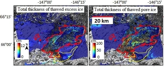
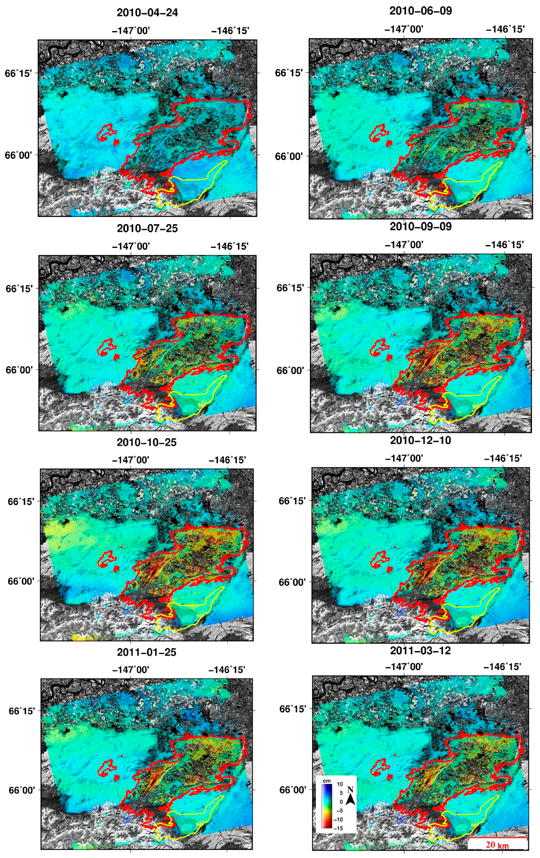
Our study area, located in the Yukon Flats, is underlain by more than 88 m of quiet-water silt and silty sand, overlain by alluvial deposits [47]. An extensive mantle of eolian silt covers the marginal upland bordering the Yukon Flats [48]. The loess, which covers the study area, is massive well-sorted homogeneous unconsolidated tan to gray silt and sandy silt [47]. Therefore, we set Ø to be 0.46 (the porosity of silt) and solved Equations 5 and 6. Figure 6 illustrates the total thickness of thawed excess ice and pore ice permafrost during the second post-fire thaw season. Figure 6a illustrates up to 15 cm depression due to excess ice permafrost degradation. Also, Figure 6b shows up to 80 cm increase in ALT during the second post-fire year.
Here, the assumption is that the post-fire soil of thawed pore-ice permafrost is fully saturated. However, this assumption may not be correct in cases where, for example, permafrost disappears entirely and becomes permeable for meltwater. Also, the equations assume that the change in the InSAR-detected organic layer deformation between the two post-fire following years, due to vegetation regrowth and soil moisture, is negligible. The change in the volume of the seasonally segregated ice between the first and second post-fire freezing seasons is assumed to be negligible. However, this assumption may not be true. Yet the main limitation of the model is related to data availability. Estimating seasonal deformations over a thawing/freezing season requires a connected network of interferograms, spanning over the entire thawing/freezing season and covering soil thaw and freeze onset dates. Sometimes, long repeat-pass periods and loss of coherence and/or other artifacts like ionospheric effect reduce the number of available interferograms. In some cases, the available network of interferograms partly covers the full season. In this case, to estimate full-season deformation using a truncated interferogram network, the modified version of the Stefan equation (explained e.g., in [9,21]) can be used to approximate the depths of thaw and freeze as a function of time and temperature.
Generally, for time series purposes, InSAR measurements are always considered to be relative to a reference point, which is assumed to have no or a predefined deformation time series. However, selecting a reference point can be controversial, and if not properly selected, a non-stable reference point will lead to biased measurements. Not that the bias initiated by using a reference point with seasonal deformations can be completely cancelled out by our model if the reference point has equal frost heave and thaw settlement in winter and summer, respectively. However, in the case of non-equal seasonal deformations of the reference point, i.e., non-equal summer subsidence and winter uplift, the model cannot fully prevent biased measurements.
4.2. Validation of InSAR Results and Estimation of Uncertainties
We selected interferograms with no ionospheric effects and the interferograms were flattened, atmospheric correction was applied to remove stratified tropospheric artifacts, and topography phase components have been removed using TanDEM-X DEM. Despite that, the measured InSAR phase may still have contributions from troposphere, topography, ionosphere, DEM errors, etc. Note that the estimated error in and , due to orbit drift are 0.04 and 0.27 cm. Also, the accuracy of phase unwrapping influences directly the accuracy of InSAR estimations. This is the case especially over low coherence pixels. So we carefully selected high coherence interferograms to avoid unwrapping error.
Here, we present the mean annual deformation velocity to visually inspect the deformations and compare the deformations over fire scar with the deformations over off-scar surrounding areas. Figure 7 presents the mean annual velocity map. Off-scar areas have less than 2-cm deformations, which is most likely induced by ground surface processes over permafrost. Also, the study area is almost flat and DEM-induced error is expected to be negligible.
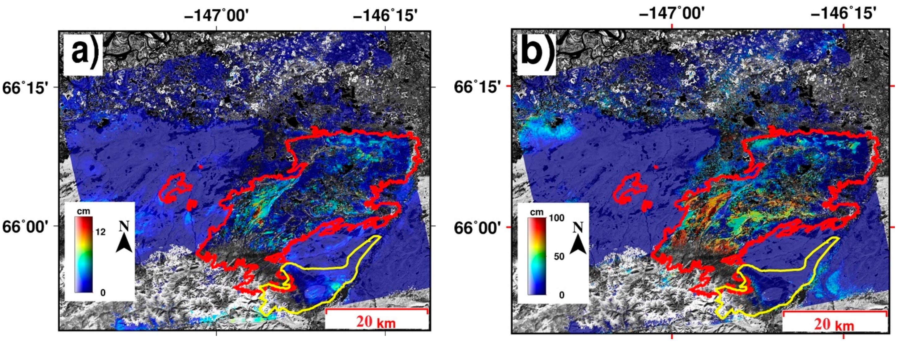
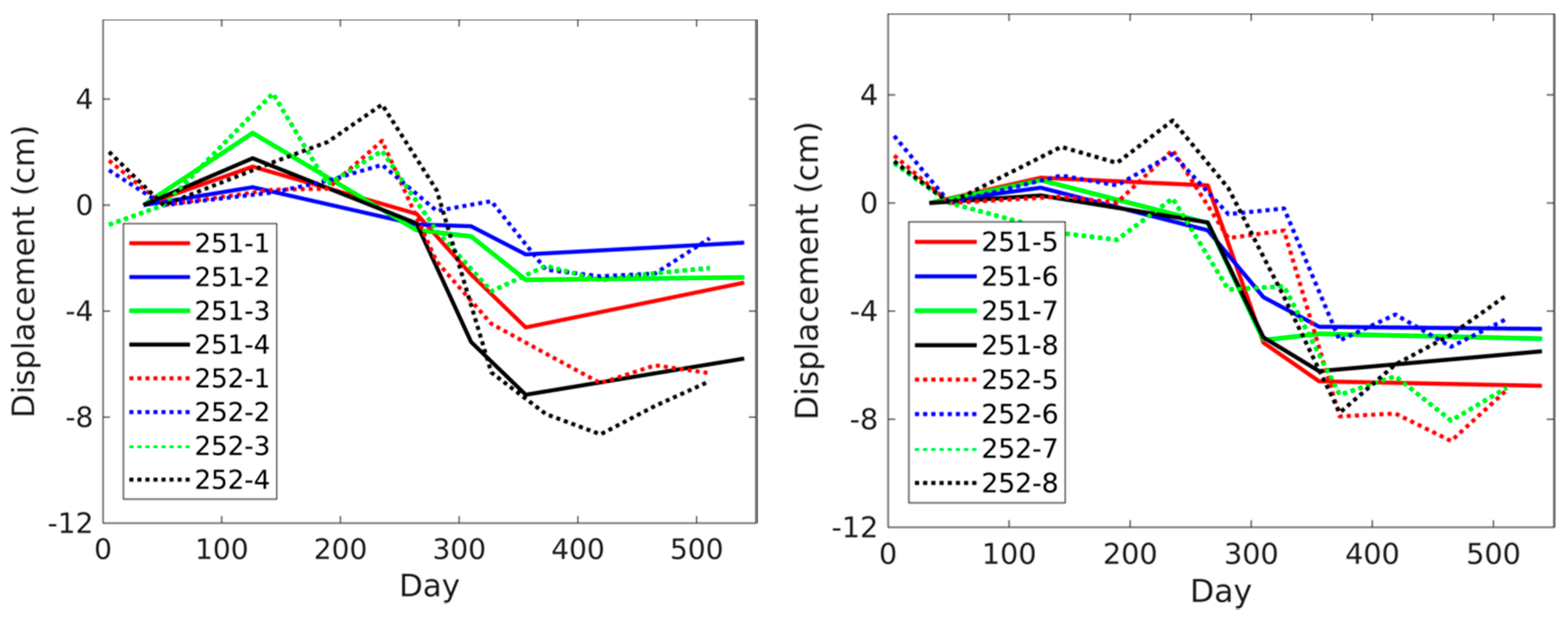
To further evaluate the InSAR results, we generated deformation time series using eight post-fire SAR images from path 251, which overlaps path 252 and covers the fire scar. Then, the results of the two independent time series from path 251 and 252 were compared by selecting eight points over the burned area (Figure 1). Figure 8 shows the plots of deformation time series over the two paths. The comparison showed good agreement between the results. Although points 2 and 3 (P251-2, P251-3, P252-2, and P252-3 in Figure 8) are on the burned area, they have smaller subsidence than other points on the burned area. This may indicate that underground permafrost was either absent or totally destroyed during the first post-fire thawing season, or that the post-fire organic layer was thick enough to keep the permafrost cool. This conclusion can be applied to all other points inside the burned area with small subsidence.
A careful inspection of the deformation time series demonstrated in Figure 5 and the model’s results shown in Figure 6 reveals that the density of low coherence pixels, i.e., colorless pixels on the images, is higher over the central and eastern part of the fire scar. Not surprisingly, the area is dominated by lakes/ponds (Figure 1). This may infer that the area is more dynamic compared to the rest of the study area and experiences surface processes that lead to the loss of coherence, which makes InSAR measurements infeasible. The rest of the area, however, possesses relatively higher coherence values. Over the higher coherence area (away from the lake/pond area), our model estimates up to a 15-cm ground level decline and up to an 80-cm increase in ALT.
Although there is no extensive ground truth data taken from the study area, we generally compared our model’s results and limited field measurements in the study area taken from 2010 to 2012 [49]. Thaw depths have been measured from 2010 to 2012 along two 100–200-m transects with different fire disturbance histories. Figure 1 shows the location of the sampling site, which is unfortunately located in the low coherence area. The measurements showed that the wildfire-increased ALT with most settlements happened during the first and second year after fire, and the permafrost table was largely stabilized in the third year after fire [49]. From 2010 to 2012, ALT increased by an average of 41 cm, with a maximum of 75 cm, and ground surface elevations declined on average by 9 cm, with a maximum of 39 cm, due to the degradation of ice-rich permafrost [49]. However, since the sampling site falls in the low coherence area, which makes InSAR measurements infeasible, we could only compare the results generally.
In general, the InSAR-estimated ground surface depression over the area away from lakes/ponds is smaller than the ground surface elevation decline measured in the lake/pond dominated area. This may indicate to us that the lake/pond dominated area is underlain by thicker excess ice permafrost. Also, our model shows up to an 80- and 40-cm increase in ALT over the southern and northern parts of the fire scare, respectively, during the first year after the fire. The estimated increase in ALT over the northern part of the study area is in good agreement with the result of ground measurements, i.e., a maximum of a 75-cm increase in ALT from 2010 to 2012 [49]. Since the thawing of excess ice permafrost did not add to ALT whereas pore ice permafrost thawing increased ALT, we can infer that the ground ice underlying the area away from the lakes/ponds, especially the southern part of the study region, is dominated by pore ice permafrost. The large increases over the southern part, i.e., up to 80 cm, indicate the likely formation of talik. However, no sample has been taken from the southern part of the fire scar to allow us to evaluate the results.
Model uncertainty can be estimated by calculating the uncertainty of each parameter involved in modeling and the sensitivity of the model to changes in the parameter, i.e., the adjoint relative to the parameter. By assuming that the parameters are affecting the model independently, the uncertainty of the model was then calculated by (e.g., [21])
where σmodel is the uncertainty of the model, Pk denotes parameters, n is the number of parameters, is the sensitivity of the model to the changes in parameter Pk, and σk represents uncertainty of Pk. Table 1 represents the parameters involved in estimating the change in the ALT, their values, uncertainties, relative contribution to the total uncertainty of the model, and cumulative uncertainties.
Equation 3 represents the parameters involved in estimating the changes in the ALT, i.e., . The value for was calculated by averaging the difference between the post-fire first and second year seasonal uplifts over the fire-affected area. The uncertainty in the parameter is the standard deviation of the difference between the post-fire first and second year seasonal uplifts over the off-scar areas. Parameter S denotes the saturation of the soil that has been added to the active layer in the second thawing season due to thawed pore ice permafrost. We assumed the soil to be fully saturated, S = 1.0. Taking porosity to be a constant value is a source of uncertainty as it is a site-specific characteristic of soil and should ideally be determined from in situ measurements at all InSAR pixels, thus we choose 0.1 of uncertainty in S. However, based on [47,48], we estimated the porosity, P, to be in a narrow range around 0.46, i.e., 0.46 ± 0.10. The uncertainty in , thawed excess ice permafrost, equals the uncertainty of the parameter . The uncertainty in the parameter is the standard deviation of the difference between the post-fire second year seasonal subsidence and uplift over the off-scar areas, i.e., 1.50 cm. Calculating standard deviation over the unburned area means that we have taken into account the uncertainties due to other sources of noise and artifacts such as long-term deformation trend, atmospheric artifacts, orbit drift, and residual orbital errors.
5. Conclusions
InSAR analyses using L-band ALOS PALSAR images have successfully mapped fire-induced permafrost deformations in interior Alaskan boreal forest where loss of coherence is a major obstacle for applying InSAR. The loss of coherence caused by wildfire was prominent within the burned area for interferograms pairing both pre- and post-fire SAR images. Although the loss of coherence restricted the total number of viable coherence pairs, by selecting only post-fire interferograms, we were able to establish interferogram networks covering three post-fire freezing and thawing seasons (2009–2010 and 2010–2011 freezing seasons, and 2010 thawing season) and generate post-fire deformation time series.
Our analyses showed that the 2009 fire caused up to 20 cm of subsidence in the thawing season of 2010. The fire increased active layer thickness, which manifested as greater uplift over burned areas compared to unburned areas. Although the permafrost process is complex, we used a simple model that uses deformation time series to estimate fire-induced change in ALT as well as the thickness of thawed excess ice permafrost. The model assumes that deformation happens because ground water takes up to 9% less volume than ground ice.
Our model revealed up to 15 cm of wildfire-induced excess ice permafrost thawing and up to an 80-cm increase in ALT. It can be seen on the map (Figure 5 and Figure 6) that except for some local patches, almost the entire burned area features ground surface subsidence due to ALT change. This indicates that almost the entire area is underlain by pore ice permafrost. The thawing of excess ice permafrost does not add to ALT, whereas pore ice permafrost thawing increases ALT and its seasonal deformations. It should be noted that ALT is usually measured from the soil surface down and not relative to the original soil surface (e.g., [32]). Therefore, we can infer that the area is dominated by pore ice permafrost. Some areas underlain by both pore and excess ice permafrost, however, experienced permafrost degradation in addition to ALT change.
A comparison between the results of path 252 and a neighboring track covering the burned area, i.e., path 251, showed a good agreement between the results of the two paths. We also estimated the uncertainty of the model by calculating the uncertainty of all parameters involved in the model. The uncertainties in the estimated change in the ALT and the thickness of the thawed excess-ice permafrost are 27.77 cm and 1.50 cm, respectively.
The introduced model can be used in other places to estimate fire-induced permafrost degradation and ALT change. However, as discussed earlier in the paper, uncertainties are involved in the model and affect the accuracy of estimated thicknesses. Therefore, pre-and post-fire extensive field sampling in an area, if available, can calibrate the model and improve the results.
Acknowledgments
The ALOS PALSAR data was downloaded from the Alaska Satellite Facility (https://www.asf.alaska.edu/). The high resolution DEM data of the study area, TanDEM-X, were provided by the German Aerospace Center (DLR). This research was financially supported by NASA Earth and Surface Interior Program (NNX16AK56G), U.S. Geological Survey (G14AC00153), and the Shuler-Foscue Endowment at Southern Methodist University. Comments and edits by the academic editor, six anonymous reviewers and Thomas Adamson significantly improved the manuscript.
Author Contributions
Yusuf Eshqi Molan processed the SAR data into InSAR products and derived time-series deformation maps, conducted modeling, and created the first draft of the manuscript. Jin Woo Kim, Zhong Lu, Bruce Wylie and Zhiliang Zhu helped interpret the results. All contributed to the writing of this manuscript.
Conflicts of Interest
The authors declare no conflict of interest. Readers who are interested in the data and products from this study can contact directly the corresponding author at the Southern Methodist University ([email protected]).
References
- Zhang, Z.Q.; Wu, Q.B. Predicting changes of active layer thickness on the Qinghai-Tibet Plateau as climate warming. J. Glaciol. Geocryol. 2012, 34, 505–511. (In Chinese) [Google Scholar]
- Zhang, T.; Barry, R.G.; Knowles, K.; Heginbottom, J.A.; Brown, J. Statistics and characteristics of permafrost and ground ice distribution in the Northern Hemisphere. Polar Geogr. 1999, 147, 169. [Google Scholar] [CrossRef]
- Apps, M.J.; Kurz, W.A.; Luxmoore, R.J.; Nilsson, L.O.; Sedjo, R.A.; Schmidt, R.; Simpson, L.G.; Vinson, T.S. Boreal forests and tundra. Water Air Soil Pollut. 1993, 70, 39–53. [Google Scholar] [CrossRef]
- Strauss, J.; Schirrmeister, L.; Wetterich, S.; Borchers, A.; Davydov, S.P. Grain-size properties and organic-carbon stock of yedoma ice complex permafrost from the Kolyma lowland, northeastern Siberia. Glob. Biogeochem. Cycles 2012, 26. [Google Scholar] [CrossRef]
- Harris, S.A.; French, J.A.; Heginbottom, G.H.; Johnston, B.; Ladanyi, D.C.; van Sego, R.O.S. Glossary of Permafrost and Related Ground-Ice Terms; Technical Memorandum No. 142, National Research Council of Canada: Ottawa, ON, USA, 1998. [Google Scholar]
- Streletskiy, D.A.; Shiklomanov, N.I.; Nelson, F.E. Spatial variability of permafrost active-layer thickness under contemporary and projected climate in northern Alaska. Polar Geogr. 2012, 35, 95–116. [Google Scholar] [CrossRef]
- Mackay, J.R. Probing for the bottom of the active layer. In Report of Activities, Part A; Geological Survey of Canada: Ottawa, ON, Canada, 1977; pp. 327–328. [Google Scholar]
- Hubbard, S.S.; Gangodagamage, C.; Dafflon, B.; Wainwright, H.; Peterson, J.; Gusmeroli, A.; Ulrich, C.; Wu, Y.; Wilson, C.; Rowland, J.; et al. Quantifying and relating land-surface and subsurface variability in permafrost environments using LiDAR and surface geophysical datasets. Hydrogeol. J. 2013, 21, 149–169. [Google Scholar] [CrossRef]
- Liu, L.; Schaefer, K.; Zhang, T.; Wahr, J. Estimating 1992–2000 average active layer thickness on the Alaskan North Slope from remotely sensed surface subsidence. J. Geophys. Res. 2012, 117. [Google Scholar] [CrossRef]
- Nelson, F.E.; Shiklomanov, N.I.; Mueller, G.R.; Hinkel, K.M.; Walker, D.A.; Bockheim, J.G. Estimating active-layer thickness over a large region: Kuparuk River basin, Alaska, USA. Arct. Alp. Res. 1997, 29, 367–378. [Google Scholar] [CrossRef]
- Shiklomanov, N.; Nelson, F. Analytic representation of the active layer thickness field, Kuparuk River Basin, Alaska. Ecol. Model. 1999, 123, 105–125. [Google Scholar] [CrossRef]
- Panda, S.K.; Prakash, A.; Solie, D.N.; Romanovsky, V.E.; Jorgenson, M.T. Remote sensing and field-based mapping of permafrost distribution along the Alaska Highway corridor, interior Alaska. Permafr. Periglac. Process. 2010, 21, 271–281. [Google Scholar] [CrossRef]
- Gangodagamage, C.; Rowland, J.C.; Hubbard, S.S.; Brumby, S.P.; Liljedahl, A.K.; Wainwright, H.; Wilson, C.J.; Altmann, G.L.; Dafflon, B.; Peterson, J.; et al. Extrapolating active layer thickness measurements across Arctic polygonal terrain using LiDAR and NDVI data sets. Water Resour. Res. 2014, 50, 6339–6357. [Google Scholar] [CrossRef] [PubMed]
- Schaefer, K.; Liu, L.; Parsekian, A.; Jafarov, E.; Chen, A.; Zhang, T.; Gusmeroli, A.; Panda, S.; Zebker, H.A.; Schaefer, T. Remotely sensed active layer thickness (ReSALT) at Barrow, Alaska using interferometric synthetic aperture radar. Remote Sens. 2015, 7, 3735–3759. [Google Scholar] [CrossRef]
- Massonnet, D.; Feigl, K. Radar interferometry and its application to changes in the Earth’s surface. Rev. Geophys. 1998, 36, 441–500. [Google Scholar] [CrossRef]
- Bürgmann, R.; Rosen, P.A.; Fielding, E.J. Synthetic aperture radar interferometry to measure Earth’s surface topography and its deformation. Annu. Rev. Earth Planet. Sci. 2000, 28, 169–209. [Google Scholar] [CrossRef]
- Simons, M.; Rosen, P. Interferometric Synthetic Aperture Radar Geodesy. Treatise Geophys. Geodesy 2007, 3, 391–446. [Google Scholar]
- Lu, Z.; Dzurisin, D. InSAR Imaging of Aleutian Volcanoes: Monitoring a Volcanic arc from Space; Geophysical Sciences; Springer Praxis Books; Springer: Chichester, UK, 2014; p. 390. [Google Scholar]
- Kim, J.; Lu, Z.; Gutenberg, L.; Zhu, Z. Characterizing hydrologic changes of the Great Dismal Swamp using SAR/InSAR. Remote Sens. Environ. 2017, 198, 187–202. [Google Scholar] [CrossRef]
- Rykhus, R.; Lu, Z. InSAR detects possible thaw settlement in the Alaskan Arctic Coastal Plain. Can. J. Remote Sens. 2008, 34, 100–112. [Google Scholar] [CrossRef]
- Liu, L.; Zhang, T.; Wahr, J. InSAR measurements of surface deformation over permafrost on the North Slope of Alaska. J. Geophys. Res. 2010, 115. [Google Scholar] [CrossRef]
- Short, N.; Brisco, B.; Couture, N.; Pollard, W.; Murnaghan, K.; Budkewitsch, P. A comparison of TerraSAR579 RADARSAT-2 and ALOS-PALSAR interferometry for monitoring permafrost environments, case study from Herschel Island, Canada. Remote Sens. Environ. 2011, 115, 3491–3506. [Google Scholar] [CrossRef]
- Liu, L.; Schaefer, K.; Gusmeroli, A.; Grosse, G.; Jones, B.M.; Zhang, T.; Parsekian, A.D.; Zebker, H.A. Seasonal thaw settlement at drained thermokarst lake basins, Arctic Alaska. Cryosphere 2014, 8, 815–826. [Google Scholar] [CrossRef] [Green Version]
- Liu, L.; Schaefer, K.M.; Chen, A.C.; Gusmeroli, A.; Zebker, H.A.; Zhang, T. Remote sensing measurements of thermokarst subsidence using InSAR. J. Geophys. Res. Earth Surf. 2015, 120, 1935–1948. [Google Scholar] [CrossRef]
- Liu, L.; Jafarov, E.E.; Schaefer, K.M.; Jones, B.M.; Zebker, H.A.; Williams, C.A.; Rogan, J.; Zhang, T. InSAR detects increase in surface subsidence caused by an arctic tundra fire. Geophys. Res. Lett. 2014, 41, 3906–3913. [Google Scholar] [CrossRef]
- Iwahana, G.; Uchida, M.; Liu, L.; Gong, W.; Meyer, F.J.; Guritz, R.; Yamanokuchi, T.; Hinzman, L. InSAR Detection and Field Evidence for Thermokarst after a Tundra Wildfire, Using ALOS-PALSAR. Remote Sens. 2016, 8, 218. [Google Scholar] [CrossRef]
- Jones, B.M.; Grosse, G.; Arp, C.D.; Miller, E.; Liu, L.; Hayes, D.J.; Larsen, C.F. Recent Arctic tundra fire initiates widespread thermokarst development. Sci. Rep. 2015, 5, 693. [Google Scholar] [CrossRef] [PubMed] [Green Version]
- Lutes, D.C.; Keane, R.E.; Caratti, J.F.; Key, C.H.; Benson, N.C.; Sutherland, S.; Gangi, L.J. FIREMON: Fire Effects Monitoring and Inventory System; General Technical Reports RMRS-GTR-164; U.S. Department of Agriculture, Forest Service, Rocky Mountain Research Station: Fort Collins, CO, USA, 2006.
- Parks, S.A.; Dillon, G.K.; Miller, C. A new metric for quantifying burn severity: The relativized burn ratio. Remote Sens. 2014, 1827–1844. [Google Scholar] [CrossRef]
- Jorgenson, M.T.; Yoshikawa, K.; Kanveskiy, M.; Shur, Y.; Romanovsky, V.; Marchenko, S.; Grosse, G.; Brown, J.; Jones, B. Permafrost characteristics of Alaska. In Proceedings of the Ninth International Conference on Permafrost Extended Abstracts, Potsdam, Germany, 20–24 June 2016; Kane, D.L., Hinkel, K.M., Eds.; University of Alaska: Fairbanks, AK, USA, 2008; pp. 121–122. [Google Scholar]
- Spetzman, L.A. Terrain Study of Alaska, Part 5. Vegetation (Map); Engineer Intelligence Study; U.S. Army, Office of Chief Engineers: Washington, DC, USA, 1963.
- Pastick, N.J.; Jorgenson, M.T.; Wylie, B.K.; Nield, S.J.; Johnson, K.D.; Finley, A.O. Distribution of near-surface permafrost in Alaska: Estimates of present and future conditions. Remote Sens. Environ. 2015, 168, 301–315. [Google Scholar] [CrossRef]
- Viereck, L.A.; Dyrness, C.T.; Batten, A.R.; Wenzlick, K.J. The Alaska Vegetation Classification; General Technical Report PNW-GTR-286; Department of Agriculture, Forest Service, Pacific Northwest Research Station: Portland, OR, USA, 1992; p. 278.
- Johnstone, J.F.; Chapin, F.S.; Hollingsworth, T.N.; Mack, M.C.; Romanovsky, V.; Turetsky, M. Fire, climate change, and forest resilience in interior Alaska. Can. J. For. Res. 2010, 40, 1302–1312. [Google Scholar] [CrossRef]
- Gallant, A.L.; Binnian, E.F.; Omernik, J.M.; Shasby, M.B. Ecoregions of Alaska US Geological Survey Professional Paper; US Department of Interior: Washington, DC, USA, 1995; p. 1567.
- Hetland, E.A.; Muse, P.; Simons, M.; Lin, Y.N.; Agram, P.S.; Di Caprio, C.J. Multiscale InSAR Time Series (MInTS) analysis of surface deformation. J. Geophys. Res. Solid Earth 2012, 117. [Google Scholar] [CrossRef]
- Lu, Z.; Wicks, C.; Kwoun, J.O.; Power, J.A.; Dzurisin, D. Surface deformation associated with the March 1996 earthquake swarm at Akutan Island, Alaska, revealed by C-band ERS and L-band JERS radar interferometry. Can. J. Remote Sens. 2005, 31, 7–20. [Google Scholar] [CrossRef]
- Costantini, M. A novel phase unwrapping method based on network programming. IEEE Trans. Geosci. Remote Sens. 1998, 36, 813–821. [Google Scholar] [CrossRef]
- Berardino, P.; Fornaro, G.; Lanari, R.; Sansosti, E. A new algorithm for surface deformation monitoring based on small baseline differential interferograms. IEEE Trans. Geosci. Remote Sens. 2002, 40, 2375–2383. [Google Scholar] [CrossRef]
- Gong, W.; Thiele, A.; Hinz, S.; Meyer, F.J.; Hooper, A.; Agram, P.S. Comparison of Small Baseline Interferometric SAR Processors for Estimating Ground Deformation. Remote Sens. 2016, 8, 330. [Google Scholar] [CrossRef]
- Agram, P.S.; Jolivet, R.; Riel, B.; Lin, Y.N.; Simons, M.; Hetland, E.; Doin, M.P.; Lasserrre, C. New Radar Interferometric Time Series Analysis Toolbox Released. Eos Trans. Am. Geophys. Union 2013, 94, 69–70. [Google Scholar] [CrossRef]
- Agram, P.S.; Jolivet, R.; Simons, M. Generic InSAR Analysis Toolbox (GIAnT), User Guide. 2016. Available online: http://earthdef.caltech.edu (accessed on 26 February 2017).
- Ahlberg, J.H.; Nielson, E.N.; Walsh, J.L. The Theory of Splines and Their Applications; Academic Press: New York, NY, USA, 1967; ISBN 0-12-044750-9. [Google Scholar]
- Clark, M.H.; Duffy, M.S. Soil Survey of Denali National Park Area, Alaska; Palmer, A.K., Ed.; Natural Resource Conservation Service: Washington, DC, USA, 2006; p. 822.
- Harris, S.A.; French, H.M.; Heginbottom, J.A.; Johnston, G.H.; Ladanyi, B.; Sego, D.C.; van Everdingen, R.O. Glossary of Permafrost and Related Ground-Ice Terms, Glossary of Permafrost and Related Ground-Ice Terms; Permafrost Subcommittee, Associate Committee on Geotechnical Research, National Research Council of Canada: Ottawa, ON, USA, 1988. [Google Scholar]
- Shiklomanov, N.I.; Streletskiy, D.A.; Little, J.D.; Nelson, F.E. Isotropic thaw subsidence in undisturbed permafrost landscapes. Geophys. Res. Lett. 2013, 40, 6356–6361. [Google Scholar] [CrossRef]
- Williams, J.R. Geologic Reconnaissance of the Yukon Flats District Alaska; United States Government Printing Office: Washington, DC, USA, 1962; pp. 289–331.
- Black, R.F. Eolian deposits of Alaska. Arctic 1951, 4, 89–111. [Google Scholar] [CrossRef]
- Nossov, D.R.; Jorgenson, M.T.; Kielland, K.; Kanevskiy, M.Z. Edaphic and microclimatic controls over permafrost response to fire in interior Alaska. Environ. Res. Lett. 2013, 8. [Google Scholar] [CrossRef]
Figure 1.
The map of 2009 (red) and 2005 (yellow) wildfire perimeters in the study area (The Bureau of Land Management Alaska Fire Service (http://afs.ak.blm.gov/)). The study area covered by paths 252 and 251 (ALOS) are boxed in cyan and green, respectively. Points P1, P2, P3, P4, P5, P6, P7, and P8 are selected points to evaluate InSAR results. The reference point and the location of ground truth measurements are shown by the cyan and green stars, respectively. The area in a green polygon is densely populated by lakes and ponds. The background image of figure is a post-fire false color composite of Landsat ETM+ bands 7 (R), 4 (G), and 2 (B).

Figure 2.
ALOS coherence estimate between 17 July 2007 and 6 September 2009 (path 252). Note near zero values over the fire scare, which indicates complete loss of InSAR coherence.
Figure 2.
ALOS coherence estimate between 17 July 2007 and 6 September 2009 (path 252). Note near zero values over the fire scare, which indicates complete loss of InSAR coherence.
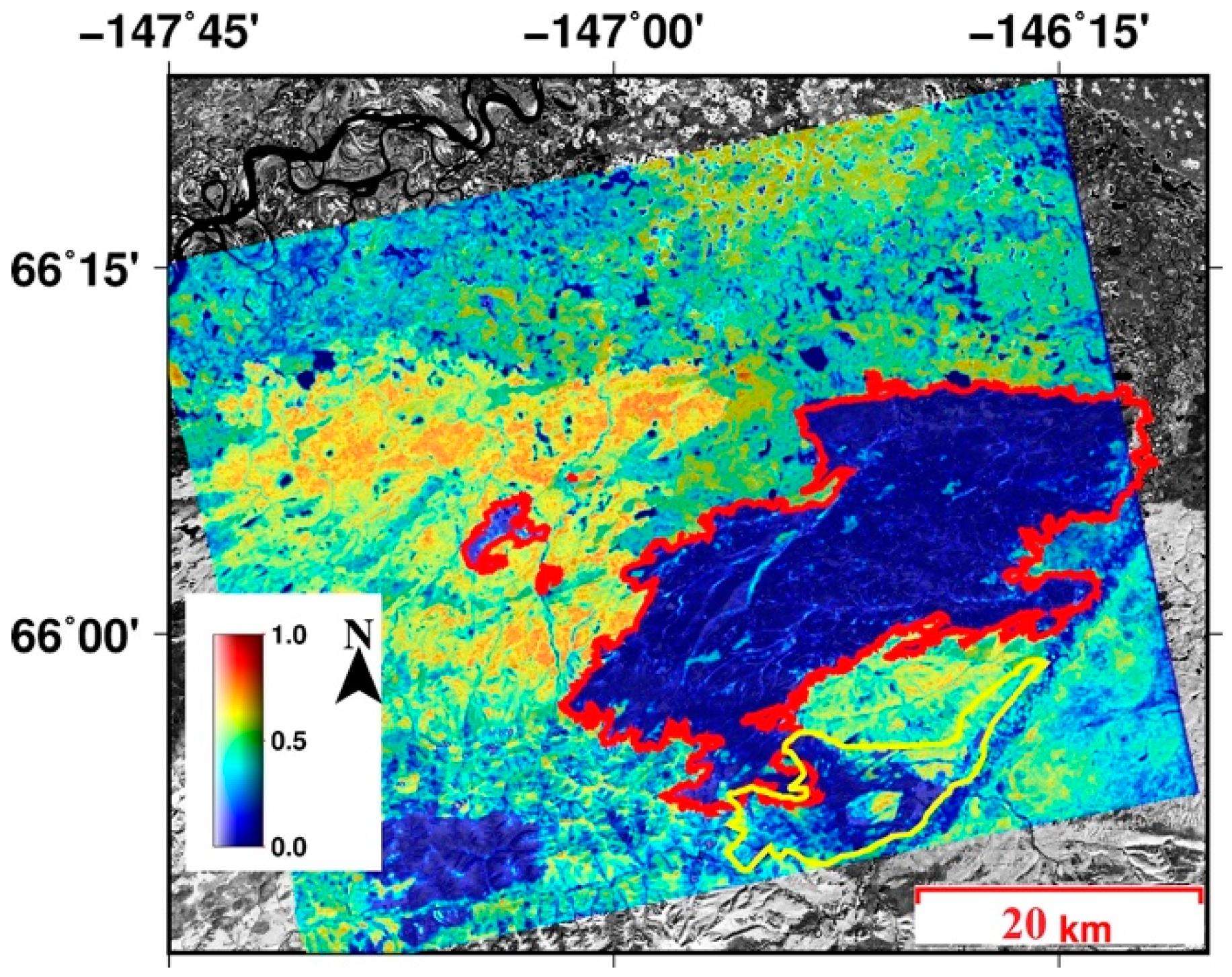
Figure 3.
Temporal and perpendicular baselines of interferograms for paths 251 and 252.

Figure 4.
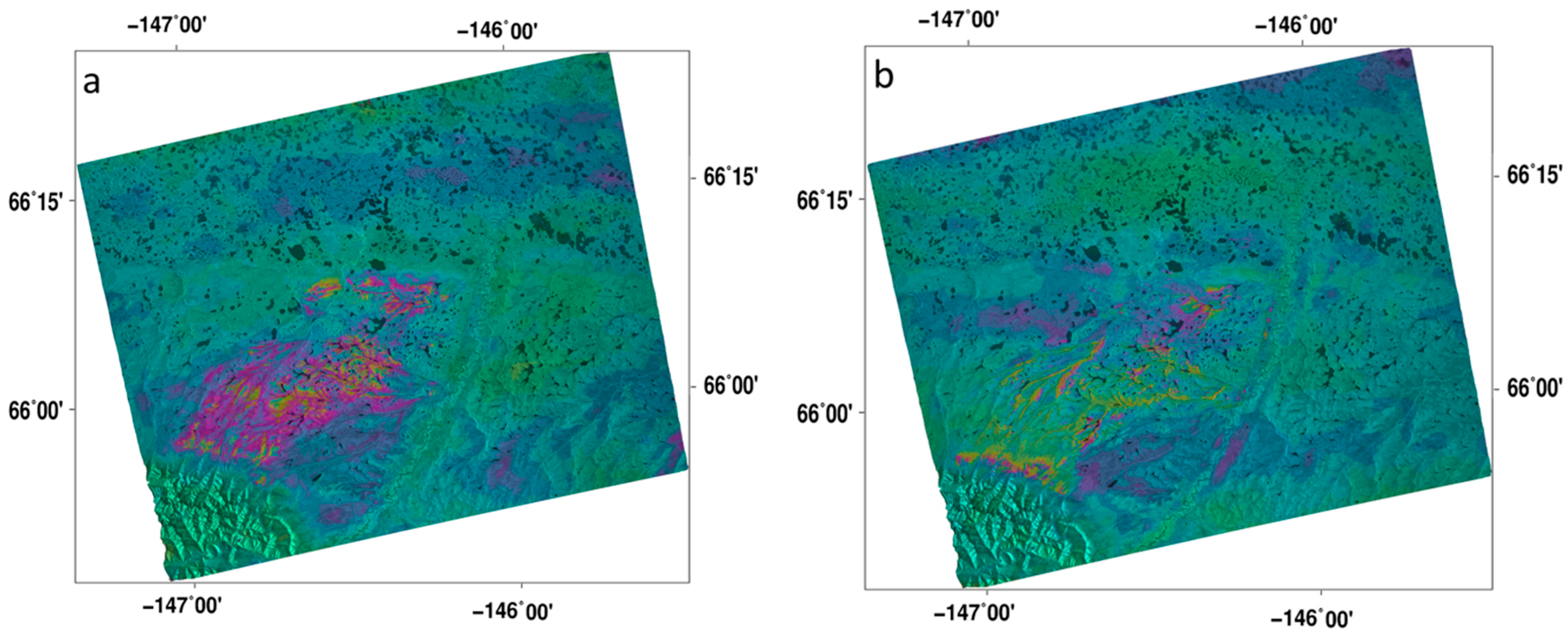
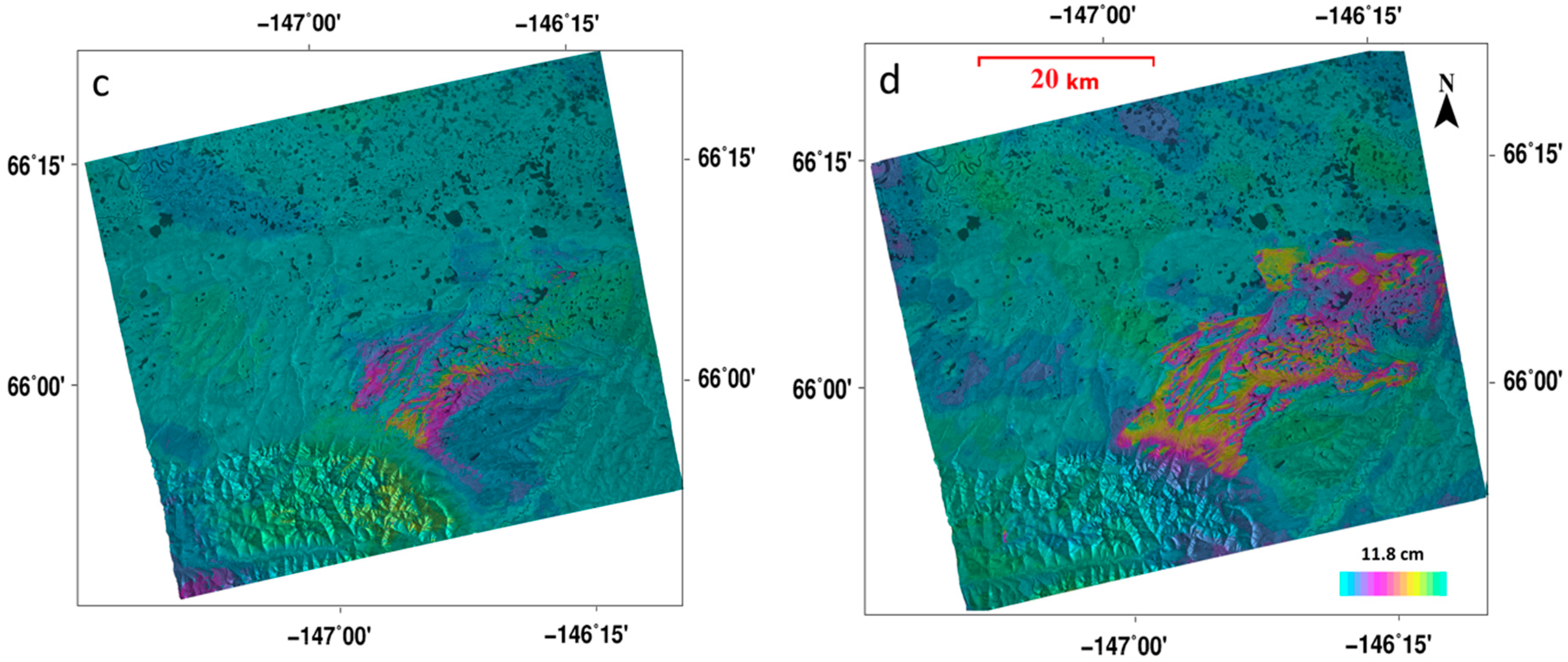
Unwrapped interferogram between images (a) 25 May 2010 and 8 July 2010 (track 251), (b) 8 July 2010 and 23 August 2010 (track 251), (c) 9 June 2010 and 25 July 2010 (track 252), and (d) 25 July 2010 and 9 September 2010 (track 252).
Figure 4.
Unwrapped interferogram between images (a) 25 May 2010 and 8 July 2010 (track 251), (b) 8 July 2010 and 23 August 2010 (track 251), (c) 9 June 2010 and 25 July 2010 (track 252), and (d) 25 July 2010 and 9 September 2010 (track 252).


Figure 5.
Accumulated deformation time series from path 252. Warm colors (red) represent ground subsidence occurring in fire-burned areas.
Figure 5.
Accumulated deformation time series from path 252. Warm colors (red) represent ground subsidence occurring in fire-burned areas.


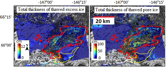
Figure 6.
Total thickness of (a) thawed excess ice and (b) pore ice permafrost during the second post-fire thaw season.
Figure 6.
Total thickness of (a) thawed excess ice and (b) pore ice permafrost during the second post-fire thaw season.

Figure 7.
Mean annual deformation velocity map of track 252.
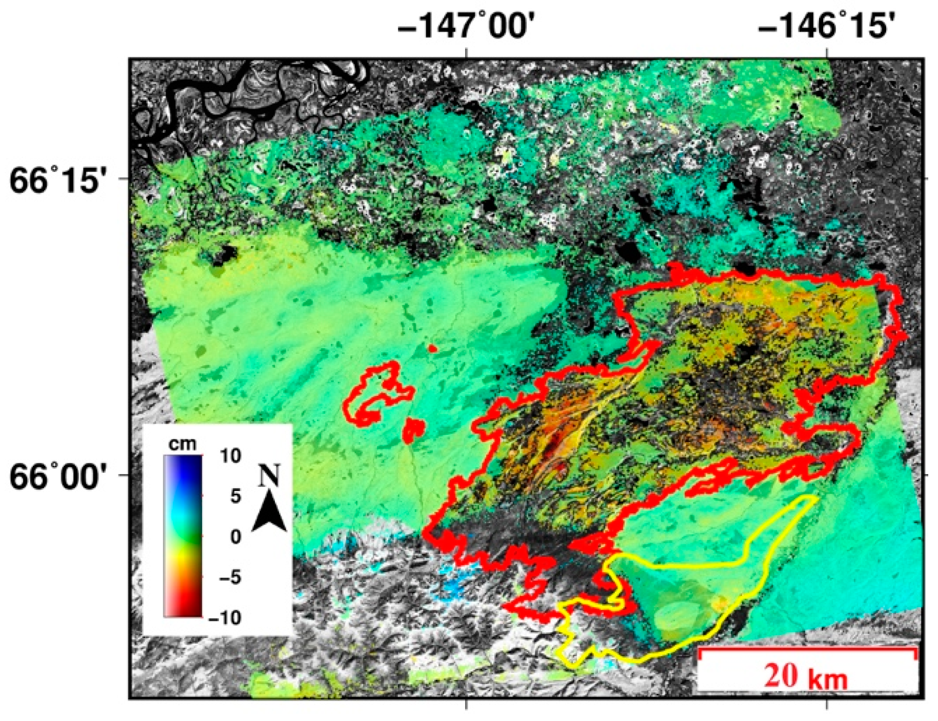
Figure 8.
Plot of deformation for the eight selected points. Each pair of the same-color solid and dotted lines represent graphs of one selected point over path 251 and 252, respectively. The x-coordinate shows days passed since 1 September 2009.
Figure 8.
Plot of deformation for the eight selected points. Each pair of the same-color solid and dotted lines represent graphs of one selected point over path 251 and 252, respectively. The x-coordinate shows days passed since 1 September 2009.


Table 1.
Model’s parameters, the uncertainties of each parameter, cumulative uncertainty, and relative contribution in the model for estimating changes in the ALT.
Table 1.
Model’s parameters, the uncertainties of each parameter, cumulative uncertainty, and relative contribution in the model for estimating changes in the ALT.
| Parameter | Value | Parameter Uncertainty | Cumulative Uncertainty (cm) | Relative Contribution (%) |
|---|---|---|---|---|
| 2.58 (cm) | 0.97 (cm) | 23.43 | 84.36 | |
| Porosity | 0.46 | ±0.10 | 27.06 | 13.09 |
| Saturation | 1.0 | 0.1 | 27.77 | 2.55 |
© 2018 by the authors. Licensee MDPI, Basel, Switzerland. This article is an open access article distributed under the terms and conditions of the Creative Commons Attribution (CC BY) license (http://creativecommons.org/licenses/by/4.0/).
Share and Cite
MDPI and ACS Style
Eshqi Molan, Y.; Kim, J.-W.; Lu, Z.; Wylie, B.; Zhu, Z. Modeling Wildfire-Induced Permafrost Deformation in an Alaskan Boreal Forest Using InSAR Observations. Remote Sens. 2018, 10, 405. https://doi.org/10.3390/rs10030405
AMA Style
Eshqi Molan Y, Kim J-W, Lu Z, Wylie B, Zhu Z. Modeling Wildfire-Induced Permafrost Deformation in an Alaskan Boreal Forest Using InSAR Observations. Remote Sensing. 2018; 10(3):405. https://doi.org/10.3390/rs10030405
Chicago/Turabian StyleEshqi Molan, Yusuf, Jin-Woo Kim, Zhong Lu, Bruce Wylie, and Zhiliang Zhu. 2018. "Modeling Wildfire-Induced Permafrost Deformation in an Alaskan Boreal Forest Using InSAR Observations" Remote Sensing 10, no. 3: 405. https://doi.org/10.3390/rs10030405
Note that from the first issue of 2016, this journal uses article numbers instead of page numbers. See further details here.