Inherent Optical Properties of the Baltic Sea in Comparison to Other Seas and Oceans


1
Department of Ecology, Environment and Plant Sciences, Stockholm University, 10691 Stockholm, Sweden
2
Bio-Optika, Crofters, Middle Dimson, Gunnislake PL18 9NQ, UK
*
Author to whom correspondence should be addressed.
Remote Sens. 2018, 10(3), 418; https://doi.org/10.3390/rs10030418
Submission received: 29 December 2017
/
Revised: 2 March 2018
/
Accepted: 4 March 2018
/
Published: 8 March 2018
(This article belongs to the Special Issue Remote Sensing of Water Quality)
Abstract
:In order to retrieve geophysical satellite products in coastal waters with high coloured dissolved organic matter (CDOM), models and processors require parameterization with regional specific inherent optical properties (sIOPs). The sIOPs of the Baltic Sea were evaluated and compared to a global NOMAD/COLORS Reference Data Set (RDS), covering a wide range of optical provinces. Ternary plots of relative absorption at 442 nm showed CDOM dominance over phytoplankton and non-algal particle absorption (NAP). At 670 nm, the distribution of Baltic measurements was not different from case 1 waters and the retrieval of Chl a was shown to be improved by red-ratio algorithms. For correct retrieval of CDOM from Medium Resolution Imaging Spectrometer (MERIS) data, a different CDOM slope over the Baltic region is required. The CDOM absorption slope, SCDOM, was significantly higher in the northwestern Baltic Sea: 0.018 (±0.002) compared to 0.016 (±0.005) for the RDS. Chl a-specific absorption and ad [SPM]*(442) and its spectral slope did not differ significantly. The comparison to the MERIS Reference Model Document (RMD) showed that the SNAP slope was generally much higher (0.011 ± 0.003) than in the RMD (0.0072 ± 0.00108), and that the SPM scattering slope was also higher (0.547 ± 0.188) vs. 0.4. The SPM-specific scattering was much higher (1.016 ± 0.326 m2 g−1) vs. 0.578 m2 g−1 in RMD. SPM retrieval could be improved by applying the local specific scattering. A novel method was implemented to derive the phase function (PF) from AC9 and VSF-3 data. was calculated fitting a Fournier–Forand PF to the normalized VSF data. was similar to Petzold, but the PF differed in the backwards direction. Some of the sIOPs showed a bimodal distribution, indicating different water types—e.g., coastal vs. open sea. This seems to be partially caused by the distribution of inorganic particles that fall out relatively close to the coast. In order to improve remote sensing retrieval from Baltic Sea data, one should apply different parameterization to these distinct water types, i.e., inner coastal waters that are more influenced by scattering of inorganic particles vs. open sea waters that are optically dominated by CDOM absorption.
1. Introduction
1.1. Description of the Baltic Sea
The Baltic Sea is a semi-enclosed sea (Figure 1) and has relatively little water exchange with the North Sea [1,2]. The high freshwater input from land combined with the relatively low input of saline bottom waters from the North Sea cause a strong halocline with saline waters at the bottom and brackish water at the top. A stable halocline is situated at about 40–70 m depth in the Baltic proper and acts as density barrier between the saline deep waters and the brackish surface waters. The deep-water salinity is about 10–13 in the Baltic Sea proper and 3–7 in the Gulf of Bothnia. There is also a strong gradient from north to south in the surface salinity across the Baltic Sea basin. Surface salinity ranges from about 1.8–3.9 in the inner Bothnian Bay, 3.8–6.6 in the Gulf of Bothnia, 5.0–11.3 in the Baltic proper, and 5.0–7.5 in the Western Gotland Sea. The renewal time for the Baltic Sea is estimated in the range of about 30–40 years [2].
Because of the relatively high freshwater input the brackish top layer is laden with coloured dissolved organic matter (CDOM), and CDOM absorption is thus by far the dominant optical component [3,4,5], both in the open Baltic Sea and in coastal waters. Højerslev et al. [6] showed that there is a strong relationship between CDOM absorption (aCDOM) and salinity across the Baltic Sea basin, but the relationships are local. There is a different aCDOM-salinity slope for salinities ranging between 2–6 (Gulf of Bothnia), 6–8 (Baltic Sea) and 8–33 (Belt Sea), respectively. Harvey et al. [7] confirmed the same for coastal areas in the Bothnian Sea and the Baltic proper. The southern Baltic Sea has some of the major rivers running into the Baltic Sea, and, due to the high run-off, the ranges of optical variables are therefore higher than in the NW Baltic Sea (see Table 1 and literature cited within). In addition, shallow areas such as the Gulf of Gdansk or the Bay of Riga have much higher ranges of optical parameters. Harvey [8] investigated the ranges of optical variables in the northwestern (NW) Baltic Sea. The ranges are similar to those in other Baltic Sea areas (Table 1).
The phytoplankton succession in the Baltic proper has a similar pattern every year. There is usually a spring bloom dominated by diatoms and dinoflagellates, and, in summer, filamentous nitrogen-fixing (diazotrophic) cyanobacteria dominate the phytoplankton, blooming mostly during July and August. In summer, a seasonal thermocline develops and the surface mixed layer (SML) reaches down to about 15–20 m depth [1], which provides another density barrier for vertical exchange. The standing stock of filamentous cyanobacteria in the Baltic proper are high in summer (about 2–4 µg L−1 Chl a) in the SML [4,21]. Chl-concentrations showed an increase of over 150% in the Northern Baltic Proper and the Gulf of Finland from the 1970s until the early 2000s, indicating eutrophication [22].
Some pelagic filamentous cyanobacteria, for example Aphanizomenon flos-aquae and Nodularia spumigena (common in the Baltic Sea), and Trichodesmium (found in the Pacific Ocean) can regulate their buoyancy due to their internal gas vacuoles [23,24] and are therefore in summer mostly restricted to the water above the thermocline and accumulate close to the surface during low wind conditions. The surface accumulations are often dominated by N. spumigena in the open Baltic Sea and can reach Chl a concentrations of >100 µg L−1 and thus are easily detected on satellite images. At high wind speeds (between 6–8 m s−1), the filaments are again mixed further down into the water column [14,25,26].
As mentioned before, the Baltic Sea is optically dominated by CDOM, but, in coastal areas, there are also significant loads of suspended particulate matter (SPM), which were shown to increase with proximity to the coast and in the inner parts of Himmerfjärden bay this increase is rather steep [4]. In the inner bay, the fraction of inorganic matter is also much higher than in the outer parts of the bay and the open sea. The inorganic SPM consists mostly of mineral particles originating from river discharge and coastal erosion. The organic fraction of SPM consists mostly of organic material, phytoplankton and bacteria [5,27,28,29,30]. In the open Baltic Sea, SPM consists almost solely of phytoplankton and/or cyanobacteria [4]. Tidal action is close to zero [1] in the Baltic Sea and, therefore, resuspension of sediments is caused mostly by wind forcing. Kuhrts et al. [31] found that sediment transport is generally smaller in summer because of lower winds. In wintertime, the wind forcing is stronger and due to the vertical mixing and enhanced vertical current shear, the resuspension of sediment is stronger. The authors also found that transport of sedimentary material over longer distances occurs only under extreme wind events that are relatively rare.
1.2. Theory of Inherent Optical Properties
The reflectance spectrum at the sea surface is influenced by the inherent optical properties (IOPs), which are absorption, scattering and the volume scattering function [32]. The total absorption coefficient, atot, is calculated as the sum of the absorption of water, aw, and the absorption coefficients of all optical in-water constituents, i.e., that of CDOM, aCDOM, phytoplankton pigments, ap, and non-algal particles, aNAP, all of which are a function of wavelength:
The total scattering coefficient, btot, in natural seawater is the sum of the scattering coefficient of water, bw, and of suspended particles, bp, all of which are a function of wavelength:
and correspondingly for the backscatter
Particulate scattering is highly anisotropic, and its geometric behavior is described by the volume scattering function (β(θ)). The integral of β over all angles is equal to total scattering coefficient, b, and the integral of the backward direction () is the backscatter coefficient bb.
The phase function is the volume scattering function normalized to the total scattering coefficient [33].
The spectral slope of the particle scatter, , is usually well represented by a power function and the spectral scatter can be described as follows:
The spectral slope of particle backscatter, , shows also a power function and can be described as follows:
Measurements of the phase function in the Baltic Sea, and other optical case 2 waters are scarce. Many studies use the Petzold Phase Function [34] to describe the volume scattering in turbid waters. The Petzold Phase Function (PF) is also used as default phase function in the MERIS RMD. The normalized backscatter ratio in natural water bodies is commonly assumed to be 0.018, the value observed by Petzold [34].
1.3. Atmospheric Correction Models
In order to derive the reflectance at the sea surface, one first needs to correct for atmospheric effects. In general, only about 10% of the reflectance signal received at top-of-atmosphere originates from the water; for the Baltic Sea, the reflectance signal amounts to only about 0.4% of the top-of-atmosphere radiance [35], which means that an accurate atmospheric correction is even more important here. For optical case 1 waters that are optically dominated by water and phytoplankton, a commonly used method is the dark pixel atmospheric correction [36]. Most coastal waters, however, are optical case 2 waters; here, the optical properties are also influenced by CDOM and SPM [37]. In these waters, the near-infrared (NIR) reflectance from the water is non-zero, which results in failure of atmospheric correction models as these do not account for the addition signal from particles in the NIR. A number of operational models have been developed to address the problem [38,39,40]. However, accurate retrieval over optical case 2 waters requires knowledge of the NIR reflectance and appropriate specific inherent optical properties (sIOPs) for the water body in question.
1.4. Forward Modelling
The marine reflectance can be derived from the inherent optical properties (forward modelling), i.e., from the scattering, absorption and the volume scattering coefficient using radiative transfer models, for example Hydrolight [41]. The air–water reflectance for diffuse irradiance, is defined as:
where nw is the refractive index of seawater, ρ is the Fresnel reflectance at normal incidence; is the Fresnel reflectance for sun and sky irradiance. Reflectance is generally dependent on the sea state for which wind speed is usually taken as a proxy.
If one has accurate spectral characterization of all optical components and the specific IOPs of a given water body, it is possible to simulate the corresponding reflectance at the sea surface, ρw, from the inherent optical properties:
where the ratio f/Q describes the bidirectional reflectance [42]. Q is the ratio of upwelling irradiance to radiance, often approximated to π allowing for the normalization of the water-leaving radiance for varying illumination and observing geometry; f is a quasi constant for case 1 waters [37].
Alternatively, for optical case 2 waters in which CDOM absorption dominates the light field, one can assume that a >> bb. Thus, atot + bbtot approximates atot and Equation (7) can be simplified as:
1.5. Retrieval of Level 2 Products via Inverse Modelling
The concentrations of the optical constituents in the water, i.e., the geophysical (level 2) products can be estimated from the reflectance at the sea surface if the specific inherent optical properties (sIOPs) of each optical component are known. The MERIS standard processor, for example, uses the reflectance at 442 nm to derive absorption and scattering at 442 nm. From this, the water products are then derived in an iterative process [43]. Examples of sIOPs are the chlorophyll-specific absorption, ap* and the particle specific scatter bp* [44,45,46]. The spectral chlorophyll-specific absorption, ap*(λ) is derived from the spectral absorption of phytoplankton, ap(λ), and normalized to the Chl a concentration [Chl a]. Likewise, the spectral SPM-specific or particle scatter, bp, is derived from the particle scatter normalized to the SPM concentration [SPM].
Previous research has shown that the Chl a concentration tends to be overestimated by the MERIS standard processor (MEGS) in the Baltic Sea whilst CDOM absorption is substantially underestimated [8,47,48,49]. This is most likely due to the fact that MEGS derives both Chl a and CDOM absorption (aCDOM + aChl) as well as particulate scatter (bp) from the reflectance at 442 nm [43,50]. SPM in turn is derived from the scatter at 442 nm, which is derived together with total absorption from level 2 reflectance. Thus, if CDOM is underestimated, the Chl a concentration (i.e., the MERIS algal-2 product in MEGS) will be overestimated. SPM can be derived very reliably by the MERIS standard processor, with a slight overestimation of only about 8–15% [48,49]. However, Chl a tends to be overestimated by about 60% [38] whilst CDOM has been consistently underestimated by 40–90% [37,49]. Thus, it is important that ocean color validation campaigns and bio-optical investigations capture the actual distribution of CDOM and the other optical in-water constituents in the Baltic Sea, as well as their specific IOPs.
An interesting solution is to use methods that train the processor on a representative range of top-of atmosphere radiances with simultaneous Chl a and SPM concentrations as well as CDOM absorption measurements. This has shown to be very effective both for the water properties processor developed by the Free University, Berlin [51]—although it does not quite fully cover the range of all optical variables representative for the Baltic Sea [49]—as well as in the empirical orthogonal functions method described by Craig et al. [52] and Wozniak et al. [53]. Both approaches work really well in the Baltic Sea [47,48,49,53]. The studies showed that one can avoid the challenges of atmospheric correction above coastal waters by training the models based on a representative set of in situ measurements. Craig et al. [52] demonstrated that already a matching set from 30 optical stations from coastal waters (Chl a and SPM concentration as well as CDOM absorption measurements along with spectral reflectance) allowed for retrieving all level 2 products reliably. This worked both using reflectance at the sea surface as well as top-of-atmosphere reflectance data derived from MERIS [53].
The main requirement for appropriate retrieval, however, is a good and representative in situ set of bio-optical properties along with reliable reflectance measurements. This is not easy to achieve as dedicated sea-truthing campaigns are very expensive and as the frequent cloud cover in the Baltic Sea makes it a challenge to get a representative match-up data set that also covers the full range of values. The FUB processor has shown superior performance in the Baltic Sea for the retrieval of Chl a [7,14,47,48,49], but it does not quite cover the full range of CDOM absorption in coastal areas of the Baltic Sea, since the training maximum for the neural network was set to 1 m−1 [51], which is not representative for Baltic Sea coastal waters. Thus, in order to reach full validity for the Baltic Sea, the FUB would have to be retrained with the full range of CDOM found in the Baltic Sea [49]. There are more recent processors such as the Case-2 Regional Coast Colour (C2RCC), which has been trained on a much wider range of coastal water types. However, Toming et al. ([54]; same special issue) tested this processor on Baltic Sea data from the Ocean and Land Colour Instrument (OLCI) that was launched on Sentinel-3 in early 2016, and their results show that the atmospheric part of the C2RCC processor performs relatively well, whilst the IOP definition of Baltic Sea waters still needs to be improved.
The aim of this study is to (i) improve the optical characterization of the Baltic Sea in order to improve the parameterization for remote sensing inversion models for coastal waters with high CDOM absorption, and to (ii) identify which of the optical properties differ significantly from other seas and oceans; and to (iii) compare the optical properties of the Baltic Sea to those implemented in the ESA MERIS reference model document (RMD) [55].
2. Materials and Methods
2.1. Baltic Data Set
The Baltic Sea data used in this paper was gathered in several dedicated Ocean Colour validation campaigns during July 2000, June 2001, August 2002, July 2008 and May 2010 [4,47,48,49] and thus covered mostly summer period dominated by filamentous cyanobacteria, but also periods of low phytoplankton standing stock (mid-May to mid-June). The summer season was the main focus of the study as the summer blooms of filamentous cyanobacteria are a main management concern for the Baltic Sea. The main area of investigation was Himmerfjärden bay in the northwestern (NW) Baltic proper, which is one of the most investigated areas in the Baltic Sea. The Baltic proper is the main water body of the Baltic Sea stretching from the Åland Sea (which borders the Gulf of Bothnia in the north) down to the Danish sounds in the southwest, excluding the Gulfs of Finland, Riga and Gdansk. Himmerfärden Bay in the NW Baltic proper acts as a recipient for the local sewage treatment plant serving approximately 800,000 people in the southern Stockholm area. It consists of several basins separated by sills and is optically dominated by CDOM, but, in the inner bay SPM concentrations, increase noticeably [4]. During the validation campaigns, optical transects were performed with 3–4 stations within each transect. The transects were either through Himmerfjärden bay (Figure 1), or from B1 offshore, towards Landsort Deep (station BY31), the deepest part of the Baltic Sea (459 m). There was a second offshore transect past the NASA Aeronet-OC station Gustaf Dahlén. About 45 of the 98 visited optical stations were located within Himmerfjärden and 13 stations were located at the coastal station B1, which is situated about 4 km southwest of Askö (Figure 1), the remaining stations were open sea stations located in the northwestern Baltic proper. Each optical stations took about 40 min, and the distance between stations varied between 7–10 km. The marine research station (Askö Laboratory) operated by Stockholm University situated on the Island of Askö close to the mouth of Himmerfjärden bay was used as a base. MERIS overpass dates and times were predicted prior to sampling using the ESOV Software Tool from the European Space Agency (Paris, France) [56], and boats and lab space were booked accordingly at Askö Laboratory [57]. During sampling, areas with surface blooms were avoided using the online information service ‘Baltic Sea Watch System’ provided by the Swedish Meteorological and Hydrological Institute [58]. The transects were cancelled in case of strong cloud cover, rain or high winds (6–8 m s−1).
The film section ‘Baltic Sea Remote Sensing’ in the film: ‘The Science of Ocean Colour’, directed by Roland Doerffer (46 min) describes the area of investigation, Askö Laboratory, and also demonstrates the optical in situ measurements during a typical transect through Himmerfjärden bay.
The film also shows the distribution of filamentous cyanobacteria in the top layers during an AC9+ profile (see methods below). The film is freely available on the Internet and can be used for academic teaching and educational purposes [59]. Some parts of the film such as optical processes under water and the deployment and functioning of optical instruments could only be explained satisfactorily by computer generated film sequences. For this purpose, the freely available software Blender was used, which is an open source project coordinated by the Blender Foundation [60]. This software has the advantage that nearly all functions can be controlled by Python scripts. The most recent version includes also an ocean simulator to produce realistic waves.
2.2. Reference Data Set
For comparison, an optical data set was merged from both the NASA NOMAD data set [61,62] and from the COLORS data set [63], which was created during the EU MAST project Coastal region long-term measurements for colour remote sensing development and validation (COLORS).
Next, a sub data set was created from these two merged data sets, including all data that, in its methodology, is most similar to the Baltic Sea data set. Figure 2 shows the geographic distribution of this reference data set (RDS).
2.3. Optical Measurements in the Baltic Sea
Absorption, scattering and the volume scattering function (VSF) were measured in situ using an AC9+ system (WetLabs, Philomath, OR, USA) fitted with a SAIV-AS STD (Bergen, Norway) and a VSF-3 (WetLabs). During measurements, the AC9+ system was handled in the same way as described in the WetLabs AC9/ACS protocol documents [64]. After taking the measurements, the data was transferred from binary to engineering units using a custom Excel program (Microsoft, Redmond, WA, USA) that applies the WetLabs calibration file (device file). A total number of 75 AC9 profiles were measured and the surface values averaged over the first two meters’ depth were included in the Baltic Sea data set. Instrument calibrations were performed by the manufacturer during 2000, 2002 and 2008. Additionally, regular lab calibrations were performed in the bio-optical laboratory at Stockholm University. Before each campaign, the AC9 was calibrated in the lab with ultrapure water as described in the WetLabs AC9/ACS protocol documents [44] in order to assure that there was no significant drift from the latest factory calibration.
The TACCS (Tethered Attenuation Coefficient Chain-Sensor; Satlantic, Halifax, NS, Canada) was used for measuring upwelling radiance and downwelling radiance and to derive reflectance. The TACCS is a radiometer system mounted on a floating buoy measuring up-welling radiance, Lu(λ), at 7 channels (412, 443, 490, 510, 560, 620 and 665 nm) situated at 50 cm below the sea surface. The TACCS system also includes 3 downwelling irradiance (Ed) sensors centered at 443, 490 and 670 nm and placed above the sea surface as well as a chain of downwelling irradiance sensors Ed (λ = 490 nm) at nominal depths of 2, 4, 6, and 8 m; all sensors have a 10 nm bandwidth. TACCS measurements were logged over 2 min (acquisition rate of 1 Hz) and at approximately 20 m away from the ship in order to avoid ship shading.
2.4. AC9 and TACCS Data Processing
The absorption and attenuation readings from the AC9 instrument were corrected for salinity and temperature using the absorption and scattering coefficients for pure water, aw(λ) and bw(λ). The values used for aw(λ) were those of Pope and Fry [65] for 400–700 nm and for 705–750 nm of Kou et al. [66]. The spectral scatter of water, bw(λ), was taken from Morel [67] and the temperature effect on spectral water absorption, δaw(λ)/δT, was derived according to Pegau and Zaneveld [68] and the effect of salinity on spectral water absorption, δaw(λ)/δS, according to Pegau et al. [69] with an update of the salinity and temperature correction according to Sullivan [70]. The absorption and scattering values for each station were then corrected for pure water from lab calibration measurements, corrected for temperature. The absorption data was corrected for scattering assuming that the absorption is a fixed proportion of the scattering [71]. Spectral scattering was derived for the nine AC9 wavebands from the difference between spectral beam attenuation and absorption.
The reflectance for testing case 2 algorithms was derived from the TACCS data using a dedicated processor [47,72], which includes a correction for instrument self-shading. For estimating upwelling radiance just below the surface, spectral Kd was derived from the AC9 spectral absorption and scatter [5] and used as an input into the TACCS processor [47,72].
Most data analysis was done in Excel. The two data basis were merged in Systat 13.1 (Systat Software, Inc., Chicago, IL, USA), which was also used for statistical data analysis and for plotting the results.
2.5. Spectral Slope of Particle Scattering
The SPM-specific scatter, i.e., the particle specific scatter, b*p [SPM] for each AC9 wavelength was derived by linear regression of vs. SPM concentration was measured gravimetrically (see below under the Section 2.7 Water samples and data analysis). The spectral slope of the particle scatter, , was derived using Equation (4) by nonlinear fitting of both data sets. Likewise, the spectral slope of particle backscatter, , was derived according to Equation (5).
2.6. Volume Scattering Function (VSF) Measurements and Calibration
The WetLabs VSF3 measures scatter in the backward direction at two wavelengths (530 nm, 660 nm) and at three angles (100°, 125°, 150°) each. The factory calibration produced unrealistic values both spectrally and in terms of scattering vs. angle. As a result, the VSF was calibrated using a silica dioxide powder (Sigma-S5631-500G, Sigma-Aldrich, St. Louis, MO, USA) that was characterized using the Multispectral Volume Scattering Meter (MVSM) developed by Lee [73]. The silica dioxide powder is a poly-disperse particulate with a particle size range of 0.5–10 μm consisting by 80% of 1–5 μm particles, which was more representative of natural sediments as compared to the polystyrene NIST-traceable bead standards used by WetLabs. The characterization from the MVSM provided a spectral VSF with an angular resolution of 2.5°. The calibration was carried out in a tank with the silica suspended in 0.2 μm reverse osmosis filtered water with the same range of SPM concentration as measured in situ and derived according to the SPM method described below (Section 2.7.2). The calibration slope determined the response of the instrument that was linear with R2 > 0.999. The zero value was calculated by linear extrapolation of the SPM values to zero concentration. The backscatter measured by the VSF was normalized by the total scatter obtained from the coincident AC9 data:
This normalized data (at three angles) was fitted to a Fournier–Forand phase function:
where , , , and is at , parameterized by relative refractive index , and the power law particle distribution using Powell minimization of the between the observed VSF (9) values and Equation (10) parameterized by . The latter is an algorithm for finding a local minimum of a function. The normalized backscatter ratio was calculated as:
by integration of the phase function. This method has the advantage that both the backscatter ratio is available and that the VSF may be estimated from the coefficients. The method suggested by WetLabs to determine bb gave a systematic error for the Baltic Sea data by a factor of 2.3592 (±0.021) R2 = 0.9966; p < 0.0001; however, there was no significant offset −0.0001 (±0.0002); p > 0.05. The spectral slope of particle backscatter from the ac-9 and VSF measurements was derived from the measurements at 530 and 620 nm for the Baltic Sea; for the RDS it was determined from the respective wavelengths available in the NOMAD data set.
2.7. Water Samples and Data Analysis
The water samples for measuring the concentrations of Chl a and SPM, and the CDOM absorption were taken from just below the surface using a dedicated sampling bucket. This method was preferred to using a sampling rosette as sampling by bucket allows for faster sampling of surface water and thus for more time to focus on the in situ optical measurements. All laboratory methods followed a standard protocol [4,26].
2.7.1. CDOM Measurements
For determining CDOM absorption in the Baltic Sea, the water was sampled in 250 mL amber glass bottles and filtered through 0.22 μm membrane filters using a Whatman glass filtration unit (with a metal mesh). The samples were transferred into 100 mL amber glass bottles and kept in the refrigerator at 20 °C until analysis and were processed within 1 month. Before scanning, the samples were removed from the refrigerator and allowed to reach room temperature before being scanned (350–850 nm) in a 10 cm optical cuvette against ultrapure water as a blank using a Shimadzu UVPC 2401 dual beam spectrophotometer (Shimadzu, Corporation, Kyoto, Japan). The spectral absorbance (abs) was then corrected for the absorbance at 700 nm in order to account for measuring errors, and the spectral absorption for CDOM, was then derived according to Kirk [5] as:
where OD(λ) is the optical density; L is the path length of the cuvette in meters (in this case 0.1 m).
CDOM absorption decreases exponentially according to the following equation [5]:
where SCDOM is the slope factor, and is the reference wavelength nominally 440 nm.
The slope factor of aCDOM was derived through nonlinear curve fitting between 412 and 510 nm (including the reference data set, see below). As such, the slope values presented here are used as a metric to compare the CDOM slope between data sets.
2.7.2. Suspended Particulate Matter
The concentration of organic and inorganic suspended matter was measured in triplicates by gravimetric analysis [74]. Whatman Glass Fiber Filters (GF/F) were rinsed with ultrapure water to remove any lose filter bits, and then combusted at 480 °C in order to burn off any possible organic contamination [50]. These clean filters were then weighed (tare filter weight) and stored in folded square aluminum foils (0.020 × 100 × 100 mm) with scored numbers until filtration. In addition, 1–2 L of water samples were filtered in triplicates through the pre-weighed and pre-combusted filters. The funnel and the filters were then rinsed with 50 mL ultrapure water to remove any remaining salt. The filters were dried overnight at 60 °C and kept in a desiccator until weighing using a microbalance (±1 µg). Total suspended matter was derived from the difference between the tare and the dry weight. Then, the samples were combusted at 480 °C in a furnace, followed by another weighing step. The weight of inorganic suspended matter equaled the weight of the combusted filters (corrected for the tare weight) and the organic fraction was derived from the difference of the total and the inorganic suspended matter. In order to correct for handling errors, 10 blank filters were processed in the same way.
2.7.3. Chlorophyll Analysis
For the estimation of chlorophyll a (Chl a), 1–2 L of sea water samples were filtered through 47 mm GF/F filters (triplicates) using a mild vacuum and stored in liquid nitrogen for a maximum of two months. For analysis, the filters were put in 10 mL 90% acetone, sonicated for 30 s, centrifuged for 10 min at 3000 RPM. After 30 min of extraction, the sample was decanted into a 1 cm quartz cuvettes and scanned against 90% acetone in a Shimadzu UVPC 2401 dual beam spectrophotometer. The Chl a concentration was then calculated according to the trichromatic method [75,76,77]. This method has been calibrated against HPLC measurements from the Norwegian Institute for Water Research (Oslo, Norway), for n = 32 sampling stations and showed no significant difference for the Chl a concentration. The measurement error was shown to be within 10% in an international inter-calibration performed by the ESA MERIS Validation Team [78].
2.7.4. Non-Algal Particle Absorption
The absorption spectra of living phytoplankton and non-algal particles (NAP) were measured spectrophotometrically using the wet filter pad technique [79]. 1–2 L of sea water were filtered through a GF/F filter. After filtration, the water-saturated filters were scanned from 350 to 750 nm using a dual beam scanning spectrophotometer (Shimadzu UV-2401) fitted with an integrated sphere. A GF/F filter saturated with ultrapure water was used as a blank in the reference light beam; for the sample filters, filtered sea water was used for saturation. The back of the integrating sphere was fitted with a plate coated with Barium sulphate, which had been provided by the manufacturer. Both filters were positioned at the entrance of the light beam into the integrating sphere with the soiled part of the sample filter positioned facing into the integrating sphere as to make sure that all scattered light by the particles on the filter would be scattered into the integrating sphere, and thus be collected and registered. After scanning the whole sample, the filter was decolorized with methanol [80]. The filter was placed on a Whatman glass filtering apparatus, 30–60 mL of methanol was added and the methanol was left to filter through by gravitation. After 30 min, the decolorized filters were rinsed with 50 mL of ultrapure water, and scanned in the same way as described above. The decolorized spectrum was corrected for the presence of phycobilin pigments (which do not extract in organic solvents) by fitting an exponential curve to the lower envelope of the spectrum from 400 to 700 nm, and thus removing the signal from the phycobilin pigment absorption. The best fit was assumed to represent the spectrum of non-algal particles, excluding the total pigment fraction (chlorophylls, carotenoids and phycobilin pigments). The decolorized spectrum was taken to be that of total non-algal particles (NAP). The difference between the initial and decolorized spectra was taken as the in vivo spectrum of the phytoplankton. All spectra were corrected for internal scattering (β-correction) by an algorithm provided by Cleveland and Weidemann [81]. The spectral optical density of the sample, OD(λ), was corrected for the optical density at 750 nm, i.e., OD’(λ) = OD(λ) − OD750. The corrected optical density, OD’(λ), was then converted to the equivalent optical density in suspension:
From this term, the absorption spectrum per unit pathlength, a(λ), was calculated:
where the factor 2.3026 converts from log10 to natural logarithm, A is the pigmented area of the filter in m2 and V the volume of the filtered sample in m3.
2.7.5. Chlorophyll-Specific Absorption and Absorption of Non-Algal Particles (NAP)
Chlorophyll-specific absorption spectra were obtained by normalizing ap to [Chl a]:
The absorption coefficient of non-algal particles (NAP) was obtained by normalizing aNAP to [SPM]:
2.7.6. aNAP Slope Calculations
NAP absorption can be approximated by a decreasing exponential function according to the following equation:
where SNAP is the slope factor, and is the reference wavelength nominally 440 nm. The slope factor of aNAP was derived through nonlinear curve fitting between 412 and 510 nm (including the COLORS and NOMAD data sets); as such, the slope values presented here are used as a metric to compare the NAP slope between data sets.
3. Results
3.1. Ranges of Optical Parameters in the Baltic Sea
Table 2 shows the comparison of the Baltic Sea and the RDS. The median [Chl a] was 3.13 μg L−1 for the Baltic Sea data set (Table 2). For the global RDS, the median [Chl a] was 0.73 μg L−1. [SPM] had a median of 1.31 g m−3 in the Baltic and 1.88 g m−3 for the global RDS. aCDOM had a median value of 0.42 m−1 in this study, which is relatively high when compared to other seas and oceans. The global RDS showed a median of 0.06 m−1 for aCDOM (Table 2).
Figure 3a shows CDOM absorption, aCDOM at 442 nm plotted against [SPM], both for the Baltic Sea data set and the reference data set. In the Baltic Sea, there is generally a large background of CDOM absorption when compared to the more global reference data set. The figure also clearly illustrates that, in the Baltic Sea, aCDOM is largely decoupled from the concentration of suspended matter, whereas, in the global data set, aCDOM is related to [SPM] to a certain extent, which is more typical for case 1 waters [37]. Figure 3b illustrates that [SPM] is also related to [Chl a], but this relationship differs for the Baltic Sea with a relatively high Chl a content in the suspended matter.
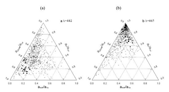
Using the measurements from the filter pad method (ap* and aNAP*) and from the spectral CDOM absorption measurements, aCDOM, the relative absorption of all optical components to total absorption was calculated and displayed as ternary plots in Figure 4a at 442 nm and Figure 4b at 665 nm. The spectral ternary plots of relative absorption of each optical component are shown for the Baltic Sea (large black diamonds) in comparison to relative absorption for the reference data set (small grey diamonds). Figure 4a clearly illustrates the relative dominance of CDOM absorption (aCDOM) in the Baltic Sea in the blue part (442 nm) of the spectrum, when compared to the relative absorption of phytoplankton (ap) and non-algal particles (aNAP). For Baltic Sea waters the variations in ap(442) are only minor compared to those in aCDOM(442), making it difficult to differentiate the Chl a absorption in the blue from CDOM absorption. However, when applying the classification instead in the red part of the spectrum (665 nm; i.e., at the Chl a absorption peak in the red), the relative absorption of phytoplankton increases substantially, and the distribution of Baltic Sea measurements even coincides with those from optical case 1 waters (Figure 4b).
3.2. Chlorophyll-Specific Absorption Derived from the Filter-Pad Method
Next, the chlorophyll-specific absorption, ap*(442) of the Baltic Sea samples was compared to the chlorophyll-specific absorption of the reference data set by plotting the phytoplankton absorption at 442 nm, ap(442) against [Chl a].
Figure 5 shows that the Baltic Sea data is placed well within the rather global data set, but the absolute Chl a absorption was somewhat placed at the higher absorption end.
The median of the chlorophyll-specific absorption, ap*(442) was 0.046 m−1 for the Baltic Sea (n = 23) with a lower quartile of 0.031 m−1 and an upper quartile of 0.064 m−1. For the RDS, ap*(442) was 0.061 m−1 with a lower quartile of 0.034 m−1 and an upper quartile of and 0.112 m−1 (n = 927).
ANCOVA analysis on log transformed data revealed that the relationship ap*(442) vs. [Chl a] does not differ significantly between the two data sets (p = 0.114).
The overall relationship was:
or in terms of a power law:
The specific absorption is thus:
The ANCOVA gave a value of −0.477 for (R2 = 0.4667), and a value of 0.5232 for for all data combined (Baltic and RDS), with a value for the Baltic of 0.6002.
3.3. Absorption of Non-Algal Particles
Next, the particle absorption at 442 nm, aNAP(442) derived from the filter pad method was plotted against the SPM concentration derived from the gravimetric method (Figure 6). The statistical analysis of the data showed that the particulate absorption at 442 nm for the Baltic Sea (0.054 ± 0.03; n = 22) was very similar to the reference data set (0.052 ± 0.32; n = 927) and did not differ significantly from the latter.
3.4. Spectral Slope of NAP and CDOM Absorption
Figure 7 shows the histograms of (a) the slope of non-algal particle absorption SNAP and (b) the slope of CDOM absorption SCDOM for the Baltic Sea data set (solid line) vs. the reference data set (dashed line). The slope of non-algal particle absorption, SNAP, had a mean value of 0.011 (±0.003) for the Baltic Sea (n = 23), which was about the same as that for the reference data set, with 0.011 (±0.002); n = 891. This compares to 0.0072 ± 0.00108 in the MERIS reference model document, meaning that the reference model document assumes very low slope values for NAP absorption when compared to both data sets. SNAP shows a bimodal distribution for the reference data set, whereas, in the Baltic Sea, it was unimodal (Figure 7a). In order to assess if the distributions differ, a Mann–Whitney test was performed. The results of the test gave a U-value of 13,046.0000 and a p-value of 0.0251, which confirms that the two distributions of SNAP differ significantly (p < 0.05).
SCDOM had a mean value of 0.018 (±0.002); n = 76 for the Baltic Sea, which is higher than that for other seas and oceans derived from the reference data set with 0.016 (±0.005); n = 860. This compares to 0.0138 (±0.00284) in the MERIS reference model document. SCDOM showed a bimodal distribution for both data sets (Figure 7b). Indicating mixing of different water masses (coastal vs. open sea). The results of the Mann–Whitney test gave a U-value of 512.0000 and a p-value of 0.0000, meaning the two distributions of SNAP differ significantly (p < 0.05).
3.5. Particle Scatter and Backscatter
For the Baltic Sea, the data set had a mean value for SPM-specific scattering of 1.016 ± 0.326 m2 g−1 (n = 56). The COLORS data set had a mean of 0.789 ± 0.90 m2 g−1 (n = 59), which does not differ significantly from the MERIS processor that uses a value of 0.578 m2 g−1. The spectral slope for particle scatter (derived from the AC9) was found to be 0.55 ± 0.19 (n = 56) for the Baltic Sea data set and 0.49 ± 0.24 (n = 82) for the reference data set (Figure 8). Thus, both the Baltic Sea data and the global reference data set indicate that the assumed slope in the MERIS RMD of 0.4 is substantially underestimated.
The mean spectral slope of backscatter, (Equation (5)), derived from the VSF measurements was higher for the Baltic Sea (1.286 ± 0.349; n = 50) than for the RDS, but the latter had a very large standard deviation (0.431 ± 1.026; n = 50) as it included a larger range of optical water types, with the distributions shown in Figure 9a. The frequency distribution of ηbb in the Baltic Sea shows a distinct peak and is bimodal, compared with the RDS, where there are fewer observations and the slope tends towards zero with a very large spread of observations. The results of the Mann–Whitney test comparing the two data sets and their distributions gave a U-value of 706.0000 and a p-value of 0.0004, confirming that the two distributions differ significantly (p < 0.05).
The spectral slope of the particle scatter, derived from the AC9 (Equation (4)) was (0.547 ± 0.188; n = 56) for the Baltic Sea and (0.49 ± 0.239; n = 82) for the RDS. Generally, the distribution of looked a bit more similar across data sets (Figure 9b), with both data sets showing a non-unimodal distribution and with a shift towards higher values for the Baltic Sea data set. The Mann–Whitney test gave a U-value of 1760.0000 and a p-value of 0.0201, and showed that the two distributions differ significantly. The different modes may indicate different water types, e.g., open sea vs. coastal data.
3.6. Backscatter Ratio and Phase Function
The analysis of the VSF3 data showed that the backscatter ratio for the Baltic Sea data was 0.0170 (±0.0103; n = 22) compared to 0.0094 (±0.0115; n = 23) for the RDS. The distribution for the Baltic Sea was bimodal—with peaks at 0.171 and 0.286 (Figure 10), indicating two distinct water types.
The results of the Mann–Whitney test gave a U-value of 326.0000 and a p-value of 0.0557, which means that they do not differ significantly. However, the test is based on rather small data sets each and the p-value is just above 0.05.
Further analysis of the phase function showed two distinct clusters of the parameters of the Fournier-Forand phase function fitted to the ac-9 and VSF data (Figure 11). The PH_1 cluster shows a higher relative refractive index ( = 1.18 ± 0.03) and lower Junge Slope ( = 3.33 ± 0.04), and has a variable , ranging from 0.03 to just below 0.01. The PH_2 cluster, however, has a lower refractive index ( = 1.03 ± 0.01) and a higher Junge Slope ( = 3.97 ± 0.10), and a more consistent , ranging from 0.02 to 0.01. Figure 11 also shows a reference line that was given by Mobley et al. [82]. It denotes a range of based on varying and values with the assumption that the lower values of can be attributed to microbes and the higher values can be attributed to mineral particles—with the Petzold PF [34] as an intermediate. The PH_1 cluster in Figure 11) shows a similar variation but with the line slightly offset. The background contours are derived from Equation (11). However, this inversion would be more appropriate from the method described in Twardowski et al. [83], which uses exact Mie computation.
3.7. Implications for Algorithms
The dominance of CDOM absorption will affect algorithms that use the blue-green ratio, such as the OC4 used by SeaWIFS, MODIS and MERIS, although the exact implementation varies between the operational processors used for these sensors. The 490 nm band is common to all these sensors and can be taken as the median blue band. We investigated this using both the RD and the Baltic data sets (Figure 13).
However, these regressions are significantly different as determined by analysis of covariance (p < 0.05), with the Baltic data showing a different slope; indicating that an OC4 type algorithm when applied to Baltic Sea waters will give an erroneous retrieval of Chl a. A number of studies have suggested the red/NIR [84] or red/green [85] algorithms may be more appropriate for coastal waters.
The reflectance ratio is significantly correlated with Chl a in log space, although the correlation is lower due to the increased noise in :
4. Discussion
The main aim of this paper was to describe the inherent optical properties of the Baltic Sea and to compare them to a global data set with the ultimate aim to improve the parameterization of semi-analytical inversion models—such as the ESA MERIS reference model—for improved retrieval of level-2 remote sensing products over Baltic Sea waters. The Baltic Sea was shown to differ in quite a few inherent optical properties, and the differences and their effect on the spectral reflectance will subsequently be discussed.
The results in this study showed rather high ranges of CDOM when compared to other seas and oceans. This has been reported in several previous studies [3,4,5,46]. In this current study, CDOM absorption ranged from 0.3–1.17 in the NW Baltic Sea with a median of 0.42 m−1. Harvey [8] measured values of up to 4.1 m−1 in the NW Baltic proper (Table 1). For the southern Baltic Sea, Wozniak et al. [53] found a range of 0.2–2.29 with a median of 0.51 m−1. For the global RDS, aCDOM was generally much lower; it ranged from 0.0012–0.64 m−1 with a median of 0.06 m−1. Similar differences were observed by Kratzer [46] who compared the optical properties of the Irish Sea and the Baltic Sea and found that there was a magnitude difference in aCDOM with the Baltic Sea showing ranges of values that were about 10-fold.
The optical dominance of CDOM in the Baltic Sea, which has been observed also in several other studies [3,4,86], makes Baltic Sea waters relatively ‘dark’ when compared to other seas and oceans. This means that they show a relatively low reflectance, especially in the blue part of the spectrum. The known inaccuracies in atmospheric correction procedures over turbid and highly absorbing waters often are exacerbated at short wavelengths, often producing erroneously low or even negative radiances and often result in overestimates of the Chl a concentrations [30,38,87,88].
However, not only the ranges of CDOM, but also its spectral slope have an influence on the retrieval of level-2 products from spectral reflectance data. In this study, there was a significant difference between the CDOM slope value derived for the Baltic Sea 0.018 (±0.002), both when compared to the global data set 0.016 (±0.005), and also when compared to the MERIS reference model document 0.0138 (±0.003), which seems extremely low. This means that the MERIS standard processor can be improved on a global scale by applying the slope value of the global data set, i.e., 0.016 (±0.005). For an improved regional Baltic Sea algorithm, the local slope value i.e., 0.018 (±0.002) should be used in order to achieve correct retrieval of CDOM absorption over NW Baltic Sea waters. Schwartz et al. [89] observed very similar ranges for CDOM slopes measured spectrophotometrically: they found that their Baltic Sea data set had a mean CDOM slope value of 0.0193 (±0.0024), where most of the measurements were from the southern Baltic Sea. Their global data set was similar (0.0164 ± 0.0035) to the combined NOMAD/COLORS RDS data set 0.016 (±0.005) but with a somewhat higher standard deviation, which is to be expected as the NOMAD/COLORS RDS was larger and also covered a larger range of optical provinces. Babin et al. [90] derived a slope value of 0.0176 (±0.002) for European waters, with the southern Baltic showing a mean of 0.019 (±0.0005). Harvey et al. [7] showed that the CDOM slope values differ slightly across Baltic Sea basins and that in coastal areas there is a rather large local variability caused by coastal gradients and due to mixing of fresh and brackish waters.
4.1. Chlorophyll-a Specific Absorption
The MERIS processor derives the Chl a concentration from the absorption at 442 nm. For this, the chlorophyll-specific absorption, ap*(442), must be known. There was a clear overlap in the values for ap*(442) from the two data basis (Baltic Sea vs. RDS) and ANCOVA on log transformed data showed that the Chl a specific absorption coefficient ap*(442) in the NW Baltic Sea did not differ significantly from the reference database. This implies that the retrieval of Chl a from remote sensing data will not be improved by applying a local conversion factor, as the relationship is generally rather scattered, due to changes in algal physiology and changes in species composition and pigment packaging.
The results of this paper showed that the median of ap*(442) was somewhat lower for the Baltic (median 0.046 m−1) than for the RDS (median 0.064 m−1). Kratzer [46] derived a median of 0.054 for ap*(442) for measurements in the open Baltic Sea around Gotland during summer 1998 (July–August; n = 12) with a min of 0.042 m−1 and maximum of and 0.063 m−1. This corresponds well to the range of the current study, which included data spanning over June–July–August with a median of 0.046 m−1 (n = 22), a lower quartile (LQ) of 0.031 m−1 and an upper quartile (UQ) of 0.064 m−1. The median ap*(442) of the RDS was 0.061 m−1 (LQ = 0.034 m−1; UQ = 0.112 m−1). This compares to a range of approximately 0.01–0.18 m−1 measured by Bricaud et al. [45] in different regions of the world oceans, where ap*(440) was shown to decrease when going from oligotrophic to eutrophic waters. This systematic shift from oligotrophic to eutrophic has also been analyzed by Roy et al. [91] using data from NOMAD and BIO data sets, and was also discussed in Babin et al. [90]. Oligotrophic waters are usually dominated by picoplanktonic species that usually have stronger pigment packaging than microplankton—which with its relative low ap*(442) dominates the Baltic Sea. The observed value of −0.477 (R2 = 0.4667) was higher than that of Bricaud et al. [45] −0.339 (R2 = 0.767) but considerably different from the value of −0.996 in the MERIS RMD; Simis et al. [92] found a value of −0.307 (R2 = 0.43). Their campaign covered both spring and summer seasons in different Baltic Sea basins, whereas the current study has a focus on the NW Baltic proper during the summer months.
4.2. Particle Absorption and Scatter
The slope of non-algal particles, SNAP, for the Baltic Sea had a mean value of 0.011 (±0.003) which was almost the same as for the reference data set (0.011 ± 0.002). This means that the value assumed in the MERIS RMD (0.0072 ± 0.00108) is far too low as it is underestimated by approximately 35%. Babin et al. [90] found a mean value for SNAP of 0.0123 (±0.0013) for European waters in general, which is very similar to our global SNAP, whereas they found a mean value of 0.013 (±0.0007) for the southern Baltic Sea.
The MERIS RMD derives SPM from the scatter at 442 nm, using the relationship:
[SPM] = b(442) × 0.578.
This means that the MERIS processor uses a value of 0.578 m2 g−1 as SPM-specific scattering. For the COLORS data set, the mean was 0.789 ± 0.90 m2 g−1 (n = 59), which does not differ significantly from the MERIS processor. For the Baltic Sea data set, however, the mean value of the SPM-specific scattering was 1.016 ± 0.326 m2 g−1 (n = 56), which, on average, is about 57% higher than the value assumed in the MERIS processor (0.578 m2 g−1). The COASTlOOC data set [93] gave a number of 0.51 m2 g−1 for the Baltic and 0.50 m2 g−1 for the complete European case 1/case 2 data set; in contrast, Woźniak et al. [68] found a value of 0.666 ± 0.321 m2 g−1 (n = 223) for the southern Baltic and the Gulf of Gdansk.
The spectral slope of particle scatter was 0.55 ± 0.19 (n = 56) for the Baltic Sea data set and 0.49 ± 0.24 (n = 82) for the reference data set. The value given in the MERIS reference model document (RMD) is a particle scatter slope of 0.4. Thus, both Baltic Sea data and the global reference data set confirm that the assumed slope in the MERIS RMD is substantially underestimated. Woźniak et al. [68] found a value of 0.404 ± 0.432 m2 g−1 (n = 223) for the southern Baltic and the Gulf of Gdansk. However, this data set had a very high standard deviation and is therefore not very conclusive.
4.3. The Phase Function in the Baltic Sea
There are only few measurements of the volume scattering function in the Baltic Sea, of these Siegel et al. [94] published the phase functions for various water types in the Baltic Sea (coastal vs. open sea). They compared their measurements to the phase function that Petzold [34] measured in turbid coastal waters (San Diego Harbor). This San Diego Harbor phase function has been used for a number of early radiative transfer studies for the MERIS RMD. It is generally referred to as the Petzold PF although a number of other measurements were in the original Petzold report. The phase functions measured by Siegel et al. [94] for various Baltic Sea coastal waters and Oder waters lie all below the Petzold PF [34], indicating that the Baltic Sea in general has a relatively low backscatter.
Our results also show that the PF are similar in shape to the Petzold PF (Figure 12a); however, in the backward direction (Figure 12b), which is more relevant for ocean color algorithms, there is a marked disparity. This would result in a lower reflectance than expected. This is presumably because of the particle size distribution expressed by the Junge slope and the particle composition, affecting the refractive index shown in Figure 11. Lying above Mobley’s reference line [82] in Figure 11, the PH_I cluster corresponds to waters containing suspended sediments with varying organic contribution and somewhat lower Chl a concentration of 3.49 (±2.54) µg L−1 when compared to 7.03 (±6.9) µg L−1 for PH_2. The waters if the PH_I cluster also shows a relatively high refractive index, indicating mineral particles. Optical investigations [4] have shown that there is a rather steep decline in mineral particles in the very inner Himmerfjärden bay.
Cluster PH_2 in Figure 11 lies below Mobley’s [82] reference line, indicating that it is dominated by microbes with a range of different size distribution and higher Chl a concentrations, but a characteristically low value of which is typical of phytoplankton. The summer blooms in the Baltic Sea are usually dominated by cyanobacteria [4], but may also include various pico- and nanoplankton and some diatom species. The values of the refractive index, and the Junge Slope. in Figure 11 can be used to generate the varying Baltic phase functions for use in radiative transfer models (e.g., Hydrolight [41]) in order to study the impact of the phase function on the upwelling light field. Generally, Figure 11 compared very well to the results published by Freda and Piskozub [95] for southern Baltic Sea water and estimated using a scattering function meter (VSM). The main difference is that in their results all measured values were spread mostly within the contours of 0.01 to 0.02, whereas the data shown in Figure 11 also spreads between the contours 0.02 to 0.03. These high values are linked to waters with a very high relative refractive index, indicating inorganic particles found in inner costal bays or very close to the shore.
4.4. Ternary Plots and Implications for Algorithms
The ternary plots shown in Figure 4 seem to be typical for the Baltic Sea region as shown in Babin et al. [90]. It must be noted though that the combined NOMAD/COLORS reference data set is much larger than the European COASTlOOC data set and contains more case 1 water types than shown in Babin et al. [90]. In the red part of the spectrum (665 nm), our RDS shows a much larger spread along the aCDOM/aTot axis. The ternary plots in the red part of the spectrum show similar results for the Baltic as for other seas and oceans when comparing ap*(665) to aCDOM(665) and aNAP*(665). Similar results have recently been published for the southern Baltic Sea [53] and by Simis et al. [92]. Thus, if one intends to use simple reflectance ratios for the retrieval of Chl a, the red/green ratio may be a viable alternative to improve the quantitative retrieval of Chl a from CDOM-dominated waters. Therefore, efforts should be made in order to derive Chl a from the reflectance signal in the red, or from the full spectrum. The results in Figure 13 show that a red to green ratio algorithm may be a viable solution if one wants to use simple ratio algorithms to derive Chl a from remote sensing reflectance data. There was no significant difference in the slopes as determined by analysis of covariance, and Figure 13b shows that the data for both the RDS and Baltic Sea data set fall on a common line. This indicates that common red/green or red/NIR algorithms could potentially be developed from both data sets combined.
However, in general, methods that use the whole reflectance spectrum usually have a better predictive power than simple reflectance ratios. Examples for this are neural network methods as applied in the MERIS standard processor [43] or the water properties processor developed by the Free University of Berlin (FUB) [51] implemented in the BEAM and SNAP ESA Earth Observations and Science Tools [96,97].
5. Conclusions
The sIOP comparison here shows that the Baltic Sea differs significantly in several sIOPs from the global data set, and from the parameterization in the MERIS Reference Document which can be improved. One of the main parameters that need improving is the slope value for CDOM SCDOM, which was significantly higher in the Baltic Sea with a mean value of 0.018 (±0.002) compared to 0.016 (±0.005) for the RDS and thus should be adjusted. As CDOM absorbs strongly in the blue, an inappropriate slope factor for CDOM will also affect Chl a retrieval in the blue as the MERIS processor derives both the absorption of Chl a and CDOM absorption from a442. The latter in turn is derived simultaneously with b442 from the remote sensing reflectance in an iterative process. The scatter at 442 nm is then used to retrieve the SPM concentration using an algorithm that was initially derived from a data set containing mostly data from the North Sea (MERIS protocols, MERIS RMD). Our analysis, however, shows that this relationship does not hold for the Baltic Sea, and that the factor in Equation (26) should be adjusted substantially, i.e., to 1.016 ± 0.326 m2 g−1—rather than 0.578 m2 g−1 as specified in the MERIS RMD. Furthermore, our results also showed that the slope value for non-algal particles, SNAP was substantially higher in the Baltic Sea (0.011 ± 0.003) than in the MERIS RMD (0.0072 ± 0.00108), and that the SPM scattering slope was also somewhat higher (0.547 ± 0.188) vs. 0.4.
SPM retrieval thus could be improved by applying the local specific scattering and the appropriate slope value. This inadequately parameterized factor for Baltic Sea waters along with an inadequate slope factor of CDOM absorption are probably some of the main explanations as to why SPM and Chl a tend to be overestimated by MEGS, while CDOM is usually underestimated [14,47,48,49]. As the retrieval of a442 and b442 from the remote sensing reflectance data, and subsequently the retrieval of CDOM, SPM and Chl a all happen in an iterative process, the retrieval of each respective level 2 parameter is linked. If one of the parameters is over- or underestimated, the retrieval of the other two parameters will be affected. Besides the above-mentioned shortcomings, another important parameter is also not well defined in the MERIS RMD, namely the phase function. The MERIS RMD applies the Petzold PF [34]. Our results show that the Petzold PF is not representative in the backwards direction for the highly absorbing waters of the Baltic Sea. This part of the phase function is crucial for the backscatter, which determines the remote sensing reflectance from which the three main optical parameters are retrieved. The contour plots in Figure 1 and the bimodal distribution of key optical variables show that we deal with two different water types—open sea vs. coastal waters indicating distinct optical regimes. Different parameterization may have to be sought for open sea and coastal waters, respectively.
Appropriate water model parameterization is not only mandatory to make better use of the existing MERIS archive (2002–2012) but also for improving the retrieval from OLCI (Sentinel-3) data. The OLCI processor is based on the experience with MERIS, and level 2 water property retrieval is also largely based on the MERIS RMD.
Acknowledgments
We thank the Swedish National Space Board (SNSB), the European Space Agency (ESA), and the FP7 project WaterS for funding this research. Thanks to Askö Laboratory staff and the members of the marine remote sensing group from Stockholm University for support during field work and Therese Harvey (Stockholm University) for additional data for Table 1. The authors extend a special thanks to all contributors to the NOMAD data set, including the NASA SIMBIOS Program (NRA-96-MTPE-04 and NRA-99-OES-09). We would like to thank our two anonymous reviewers for very constructive feedback on how to improve the paper.
Author Contributions
We confirm that both authors have contributed to the planning and the writing of the article, to the field measurements in the Baltic Sea, data processing, data analysis and the interpretation of data. Gerald Moore was mainly responsible for the data calibration and for merging the data sets while Susanne Kratzer was mainly responsible for field logistics and lab measurements and the writing. We confirm that both authors have read and accepted the final version of the manuscript.
Conflicts of Interest
The authors declare no conflict of interest.
Notation
| Abbreviation | Optical Property | Unit |
| ℜ | Air water interface term | dimensionless |
| ρw | Above water reflectance | dimensionless |
| Particulate backscattering ratio | dimensionless | |
| Relative refractive index of particles | dimensionless | |
| Normalized phase function | sr−1 | |
| The spectral slope of scattering | dimensionless | |
| The spectral slope of backscattering | dimensionless | |
| aCDOM(440) | CDOM absorption at 440 nm | m−1 |
| ad [SPM]* | SPM specific absorption | m2 g−1 |
| aNAP | Non Algal Particle absorption coefficient | m−1 |
| ap | phytoplankton absorption coefficient | m−1 |
| ap* | phytoplankton specific absorption coefficient | m2 mg−1 |
| atot | Total absorption coefficient | m−1 |
| aw | Water absorption coefficient | m−1 |
| b*p [SPM] | SPM specific scattering coefficient | m2 g−1 |
| bb*p [SPM] | SPM specific backscattering coefficient | m2 g−1 |
| bbp | Particulate backscattering coefficient | m−1 |
| bbtot | Total backscattering coefficient | m−1 |
| bbw | Water scattering coefficient | m−1 |
| btot | Total scattering coefficient | m−1 |
| f | Empirical factor relating IOPs to R | dimensionless |
| F | Empirical factor relating IOPs to ρw | dimensionless |
| f’ | Empirical factor relating IOPs to R | dimensionless |
| F’ | Empirical factor relating IOPs to ρw | dimensionless |
| nw | Refractive index of seawater | dimensionless |
| OD(λ) | Optical Density | dimensionless |
| Q | Ratio of upwelling irradiance to radiance | dimensionless |
| r | Air-water reflectance for diffuse irradiance | dimensionless |
| SCDOM | The spectral slope of CDOM absorption | dimensionless |
| SNAP | The spectral slope of NAP absorption | dimensionless |
| λ | Wavelength | nm |
| Junge slope | dimensionless | |
| ρw | Water reflectance (above surface) | dimensionless |
References
- Voipio, A. The Baltic Sea; Elsevier: Amsterdam, The Netherlands, 1981; Volume 30, p. 417. ISBN 9780080870687. [Google Scholar]
- Snoeijs-Leijonmalm, P.; Andrén, E. Why is the Baltic Sea so special to live in? In Biological Oceanography of the Baltic Sea; Snoeijs-Leijonmalm, P., Schubert, H., Radziejewska, T., Eds.; Springer International Publishing: Cham, Switzerland, 2017; pp. 23–84. ISBN 978-94-007-0668-2. [Google Scholar]
- Kowalczuk, P.; Stedmon, C.A.; Markager, S. Modelling absorption by CDOM in the Baltic Sea from season, salinity and chlorophyll. Mar. Chem. 2006, 101, 1–11. [Google Scholar] [CrossRef]
- Kratzer, S.; Tett, P. Using bio-optics to investigate the extent of coastal waters: A Swedish case study. Hydrobiologia 2009, 629, 169–186. [Google Scholar] [CrossRef]
- Kirk, J.T.O. Light and Photosynthesis in Aquatic Ecosystems, 3rd ed.; Cambridge University Press: New York, NY, USA, 1984; p. 649. ISBN 978-0-521-15175-7. [Google Scholar]
- Højerslev, N.K.; Holt, N.; Aarup, T. Optical measurements in the North Sea-Baltic Sea transition zone. I. On the origin of the deep water in the Kattegat. Cont. Shelf Res. 1996, 16, 1329–1342. [Google Scholar] [CrossRef]
- Harvey, E.T.; Kratzer, S.; Andersson, A. Relationships between colored dissolved organic matter and dissolved organic carbon in different coastal gradients of the Baltic Sea. AMBIO 2015, 44, 392–401. [Google Scholar] [CrossRef] [PubMed]
- Harvey, T. Bio-Optics, Satellite Remote Sensing and Baltic Sea Ecosystems: Applications for Monitoring and Management. Ph.D. Thesis, Department of Ecology, Environment and Plant Sciences, Stockholm University, Stockholm, Sweden, 2015. [Google Scholar]
- Ohde, T.; Siegel, H.; Gerth, M. Validation of MERIS Level-2 products in the Baltic Sea, the Namibian coastal area and the Atlantic Ocean. Int. J. Remote Sens. 2007, 28, 609–624. [Google Scholar] [CrossRef]
- Fleming-Lehtinen, V.; Laamanen, M. Long-term changes in Secchi depth and the role of phytoplankton in explaining light attenuation in the Baltic Sea. Estuar. Coast. Shelf Sci. 2012, 102, 1–10. [Google Scholar] [CrossRef]
- Kowalczuk, P.; Olszewski, J.; Darecki, M.; Kaczmarek, S. Empirical relationships between Coloured Dissolved Organic Matter (CDOM) absorption and apparent optical properties in Baltic Sea waters. Int. J. Remote Sens. 2005, 26, 345–370. [Google Scholar] [CrossRef]
- Wasmund, N.; Andrushaitis, A.; Łysiak-Pastuszak, E.; Müller-Karulis, B.; Nausch, G.; Neumann, T.; Ojaveer, H.; Olenina, I.; Postel, L.; Witek, Z. Trophic status of the South-Eastern Baltic Sea: A comparison of coastal and open areas. Estuar. Coast. Shelf Sci. 2001, 53, 849–864. [Google Scholar] [CrossRef]
- Woźniak, S.B.; Meler, J.; Lednicka, B.; Zdun, A.; Stoń-Egiert, J. Inherent optical properties of suspended particulate matter in the southern Baltic Sea. Oceanologia 2011, 53, 691–729. [Google Scholar] [CrossRef]
- Vaičiūtė, D.; Bresciani, M.; Bučas, M. Validation of MERIS bio-optical products with in situ data in the turbid Lithuanian Baltic Sea coastal waters. J. Appl. Remote Sens. 2012, 6, 063568. [Google Scholar] [CrossRef]
- Alikas, K.; Kratzer, S.; Reinart, A.; Kauer, T.; Paavel, B. Robust remote sensing algorithms to derive the diffuse attenuation coefficient for lakes and coastal waters. Limnol. Oceanogr. Methods 2015, 13, 402–415. [Google Scholar] [CrossRef]
- Alikas, K.; Kratzer, S.; Reinart, A. Robust Kd(490) and Secchi algorithms for remote sensing of optically complex waters. In Proceedings of the Ocean Optics XXI Conference, Glasgow, UK, 8–12 October 2012. [Google Scholar]
- Raag, L.; Sipelgas, L.; Uiboupin, R. Analysis of natural background and dredging-induced changes in TSM concentration from MERIS images near commercial harbours in the Estonian coastal sea. Int. J. Remote Sens. 2014, 35, 6764–6780. [Google Scholar] [CrossRef]
- Toming, K.; Arst, H.; Paavel, B.; Laas, A.; Nõges, T. Spatial and temporal variations in coloured dissolved organic matter in large and shallow Estonian water bodies. Boreal Environ. Res. 2009, 14, 959–970. [Google Scholar]
- Vazyulya, S.; Khrapko, A.; Kopelevich, O.; Burenkov, V.; Eremina, T.; Isaev, A. Regional algorithms for the estimation of chlorophyll and suspended matter concentration in the Gulf of Finland from MODIS-Aqua satellite data. Oceanologia 2014, 56, 737–756. [Google Scholar] [CrossRef]
- Koponen, S.; Attila, J.; Pulliainen, J.; Kallio, K.; Pyhälahti, T.; Lindfors, A.; Rasmus, K.; Hallikainen, M. A case study of airborne and satellite remote sensing of a spring bloom event in the Gulf of Finland. Cont. Shelf Res. 2007, 27, 228–244. [Google Scholar] [CrossRef]
- Suikkanen, S.; Laamanen, M.; Huttunen, M. Long-term changes in summer phytoplankton communities of the open northern Baltic Sea. Estuar. Coast. Shelf Sci. 2007, 71, 580–592. [Google Scholar] [CrossRef]
- Fleming-Lehtinen, V.; Laamanen, M.; Kuosa, H.; Haahti, H.; Olsonen, R. Long-term development of inorganic nutrients and chlorophyll α in the open northern Baltic Sea. AMBIO 2008, 37, 86–92. [Google Scholar] [CrossRef]
- Walsby, A.E.; Hayes, P.K.; Boje, R. The gas vesicles, buoyancy and vertical distribution of cyanobacteria in the Baltic Sea. Eur. J. Phycol. 1995, 30, 87–94. [Google Scholar] [CrossRef] [Green Version]
- Carpenter, E.J.; Capone, D.G. Marine Pelagic Cyanobacteria: Trichodesmium and Other Diazotrophs; Springer Science and Business Media: Berlin, Germany, 2013; Volume 362, ISBN 978-94-015-7977-3. [Google Scholar]
- Kahru, M.; Leppanen, J.M.; Rud, O. Cyanobacterial blooms cause heating of the sea surface. Mar. Ecol. Prog. Ser. 1993, 101, 1–7. [Google Scholar] [CrossRef]
- Subramaniam, A.; Kratzer, S.; Carpenter, J.C.; Söderbäck, E. Remote sensing and optical in-water measurements of a cyanobacteria bloom in the Baltic Sea. Best of plenary session. In Proceedings of the Sixth International Conference on Remote Sensing for Marine and Coastal Environments, Charleston, SC, USA, 1–3 May 2000. [Google Scholar]
- Jerlov, N. Marine Optics. In Elsevier Oceanography Series 14; Elsevier: New York, NY, USA, 1976; p. 231. [Google Scholar]
- Bukata, R.P.; Jerome, J.H.; Kondratyev, K.Y.; Pozdnyakov, D.V. Optical Properties and Remote Sensing of Inland and Coastal Waters; CRC Press: Boca Raton, FL, USA, 1995; ISBN 9780849347542. [Google Scholar]
- Bowers, D.G.; Binding, C.E. The Optical Properties of Mineral Suspended Particles: A Review and Synthesis. Estuar. Coast. Shelf Sci. 2006, 67, 219–230. [Google Scholar] [CrossRef]
- Binding, C.E.; Greenberg, T.A.; Jerome, J.H.; Bukata, R.P.; Letourneau, G. An assessment of MERIS algal products during an intense bloom in Lake of the Woods. J. Plankton Res. 2010, 33, 793–806. [Google Scholar] [CrossRef]
- Kuhrts, C.; Fennel, W.; Seifert, T. Model studies of transport of sedimentary material in the western Baltic. J. Mar. Syst. 2004, 52, 167–190. [Google Scholar] [CrossRef]
- Preisendorfer, R.W. Application of Radiative Transfer theory to Light Measurements in the Sea. In Proceedings of the Symposium on Radiant Energy in the Sea, International Union of Geodetic and Geophysics, Helsinki, Finland, 4–5 August 1960. [Google Scholar]
- Morel, A.; Gentili, B. Diffuse reflectance of oceanic waters: Its dependence on sun angle as influenced by the molecular scattering contribution. Appl. Opt. 1991, 30, 4427–4438. [Google Scholar] [CrossRef] [PubMed]
- Petzold, T.J. Volume Scattering Functions for Selected Natural Waters; No. SIO-REF-72-78; Scripps Institution of Oceanography La Jolla Ca Visibility Laboratory: San Diego, CA, USA, 1972; p. 77. [Google Scholar]
- Wang, M. Atmospheric correction for remotely-sensed ocean-colour products. In Reports and Monographs of the International Ocean-Colour Coordinating Group (IOCCG); IOCCG: Dartmouth, Canada, 2010; Available online: www.vliz.be/imisdocs/publications/ocrd/259206.pdf (accessed on 6 March 2018).
- Siegel, D.A.; Wang, M.; Maritorena, S.; Robinson, W. Atmospheric correction of satellite ocean color imagery: The black pixel assumption. Appl. Opt. 2000, 39, 3582–3591. [Google Scholar] [CrossRef] [PubMed]
- Morel, A.; Prieur, L. Analysis of variations in ocean color. Limnol. Oceanogr. 1977, 22, 709–722. [Google Scholar] [CrossRef]
- Moore, G.F.; Aiken, J.; Lavender, S.J. The atmospheric correction of water colour and the quantitative retrieval of suspended particulate matter in Case II waters: Application to MERIS. Int. J. Remote Sens. 1999, 20, 1713–1733. [Google Scholar] [CrossRef]
- Moses, W.J.; Gitelson, A.A.; Berdnikov, S.; Povazhnyy, V. Estimation of chlorophyll-a concentration in case II waters using MODIS and MERIS data—Successes and challenges. Environ. Res. Lett. 2009, 4, 045005. [Google Scholar] [CrossRef]
- Goyens, C.; Jamet, C.; Schroeder, T. Evaluation of four atmospheric correction algorithms for MODIS-Aqua images over contrasted coastal waters. Remote Sens. Environ. 2013, 131, 63–75. [Google Scholar] [CrossRef]
- Mobley, C.D. Hydrolight 3.0 Users Guide; SRIRI Project 5632; SRI International: Menlo Park, CA, USA, 1995; p. 65. [Google Scholar]
- Morel, A.; Antoine, D.; Gentili, B. Bidirectional reflectance of oceanic waters: Accounting for Raman emission and varying particle phase function. Appl. Opt. 2002, 41, 6289–6306. [Google Scholar] [CrossRef] [PubMed]
- Doerffer, R.; Schiller, H. The MERIS Case 2 water algorithm. Int. J. Remote Sens. 2007, 28, 517–535. [Google Scholar] [CrossRef]
- Hoepffner, N.; Sathyendranath, S. Bio-optical characteristics of coastal waters: Absorption spectra of phytoplankton and pigment distribution in the western North Atlantic. Limnol. Oceanogr. 1992, 37, 1660–1679. [Google Scholar] [CrossRef]
- Bricaud, A.; Babin, M.; Morel, A.; Claustre, H. Variability in the chlorophyll-specific absorption coefficients of natural phytoplankton: Analysis and parameterization. J. Geophys. Res. Oceans 1995, 100, 13321–13332. [Google Scholar] [CrossRef]
- Kratzer, S. Bio-Optical Studies of Coastal Waters. Ph.D. Thesis, School of Ocean Sciences, University of Wales, Bangor, UK, 2000. [Google Scholar]
- Kratzer, S.; Brockmann, C.; Moore, G. Using MERIS full resolution data (300 m spatial resolution) to monitor coastal waters—A case study from Himmerfjärden, a fjord-like bay in the northwestern Baltic Sea. Remote Sens. Environ. 2008, 112, 2284–2300. [Google Scholar] [CrossRef]
- Kratzer, S.; Vinterhav, C. Improvement of MERIS level 2 products in baltic sea coastal areas by applying the improved Contrast between Ocean and Land Processor (ICOL)—Data analysis and validation. Oceanologia 2010, 52, 211–236. [Google Scholar] [CrossRef]
- Beltrán-Abaunza, J.M.; Kratzer, S.; Brockmann, C. Evaluation of MERIS products from Baltic Sea coastal waters rich in CDOM. Ocean Sci. 2014, 10, 377–396. [Google Scholar] [CrossRef]
- Doerffer, R. Protocols for the Validation of MERIS Water Products; European Space Agency Doc. No. PO-TN-MEL-GS-0043; GKSS: Geesthacht, Germany, 2002; pp. 1–42. [Google Scholar]
- Schroeder, T.; Behnert, I.; Schaale, M.; Fischer, J. Retrieval of atmospheric and oceanic properties from MERIS measurements: A new Case-2 water processor for BEAM. Int. J. Remote Sens. 2007, 28, 5627–5632. [Google Scholar] [CrossRef]
- Craig, S.E.; Jones, C.T.; Li, W.K.W.; Lazin, G.; Horne, E.; Caverhill, C. Deriving optical metrics of coastal phytoplankton biomass from ocean colour. Remote Sens. Environ. 2012, 119, 72–83. [Google Scholar] [CrossRef]
- Woźniak, M.; Craig, S.; Kratzer, S.; Wojtasiewicz, B.; Darecki, M. A Novel Statistical Approach for Ocean Colour Estimation of Inherent Optical Properties and Cyanobacteria Abundance in Optically Complex Waters. Remote Sens. 2017, 9, 343. [Google Scholar] [CrossRef]
- Toming, K.; Kutser, T.; Uiboupin, R.; Arikas, A.; Vahter, K.; Paavel, B. Mapping Water Quality Parameters with Sentinel-3 Ocean and Land Colour Instrument imagery in the Baltic Sea. Remote Sens. 2017, 9, 1070. [Google Scholar] [CrossRef]
- ESA, Reference Model for MERIS Level 2 Processing, 3rd MERIS Reprocessing. Ocean Branch Issue 5, Rev. 4. Available online: https://earth.esa.int/documents/10174/1462454/Envisat_MERIS_RMD_Third-Reprocessing_Level-2/ (accessed on 21 February 2018).
- ESA ESOV Software Tool. Available online: https://earth.esa.int/web/guest/software-tools/-/article/esov-software-tools-esov-ng-and-esov-classic-1652 (accessed on 21 February 2018).
- Askö Laboratory, Baltic Sea Centre. Available online: http://www.su.se/ostersjocentrum/english/askö-laboratory (accessed on 21 February 2018).
- Baltic Sea Watch System (BAWS), Swedish Meteorological and Hydrological Institute (SMHI). Available online: https://www.smhi.se/klimatdata/oceanografi/algsituationen (accessed on 21 February 2018).
- The Baltic Sea Remote Sensing. The Science of Ocean Colour, a film by Roland Doerffer. Available online: http://www.spicosa.eu/setnet/downloads/ (accessed on 21 February 2018).
- Blender Open Source 3D Creation. Available online: http://www.blender.org (accessed on 21 February 2018).
- NOMAD: NASA Bio-Optical Marine Algorithm Dataset. Available online: https://seabass.gsfc.nasa.gov/wiki/NOMAD (accessed on 21 February 2018).
- Werdell, P.; Bailey, S. An improved in-situ bio-optical data set for ocean color algorithm development and satellite data product validation. Remote Sens. Environ. 2005, 98, 122–140. [Google Scholar] [CrossRef]
- Data Base if the EU MAST Project (MAS3-CT97-0087) COLORS: Coastal Region Long-Term Measurements for Colour Remote Sensing Development and Validation. Available online: http://databases.eucc-d.de/plugins/projectsdb/project.php?show=234 (accessed on 21 February 2018).
- WetLabs AC9/ACS Protocol Documents. Available online: ftp://misclab.umeoce.maine.edu/classes/OO2017/labs_resources/lab2/acprotq_ac9_protocol.pdf (accessed on 21 February 2018).
- Pope, R.M.; Fry, E.S. Absorption spectrum (380–700 nm) of pure water. II. Integrating cavity measurements. Appl. Opt. 1997, 36, 8710–8723. [Google Scholar] [CrossRef] [PubMed]
- Kou, L.; Labrie, D.; Chylek, P. Refractive indices of water and ice in the 0.65- to 2.5-µm spectral range. Appl. Optics 1993, 32, 3531–3540. [Google Scholar] [CrossRef] [PubMed]
- Morel, A. Optical properties of pure water and pure sea water. In Optical Aspects of Oceanography; Jerlov, N.G., Steemann-Nielsen, E., Eds.; Academic: New York, NY, USA, 1974; pp. 1–24. [Google Scholar]
- Pegau, W.S.; Zaneveld, J.R.V. Temperature dependent absorption of water in the red and near infrared portions of the spectrum. Limnol. Oceanogr. 1993, 38, 188–192. [Google Scholar]
- Pegau, W.S.; Gray, D.; Zaneveld, J.R.V. Absorption and attenuation of visible and near-infrared light in water: The dependence on temperature and salinity. Appl. Opt. 1997, 36, 6035–6046. [Google Scholar] [CrossRef] [PubMed]
- Sullivan, J.M.; Twardowski, M.S.; Zaneveld, J.R.V.; Moore, C.M.; Barnard, A.H.; Donaghay, P.L.; Rhoades, B. The hyperspectral temperature and salt dependencies of absorption by water and heavy water in the 400–750 nm spectral range. Appl. Opt. 2006, 45, 5294–5309. [Google Scholar] [CrossRef] [PubMed]
- Kirk, J.T.O. Monte Carlo modeling of the performance of a reflective tube absorption meter. Appl. Opt. 1992, 31, 6463–6468. [Google Scholar] [CrossRef] [PubMed]
- Zibordi, G.; Ruddick, K.; Ansko, I.; Moore, G.; Kratzer, S.; Icely, J.; Reinart, A. In situ determination of the remote sensing reflectance: An inter-comparison. Ocean Sci. 2012, 8, 567–586. [Google Scholar] [CrossRef]
- Lee, M.E.; Lewis, M.R. A New Method for the Measurement of the Optical Volume Scattering Function in the Upper Ocean. J. Atmos. Ocean Tech. 2003, 20, 563–571. [Google Scholar] [CrossRef]
- Strickland, J.H.D.; Parsons, T.R. A Practical Handbook of Sea-Water Analysis. Fisheries Research Board of Canada Bulletin 167, 2nd ed.; Fisheries Research Board of Canada: Ottawa, ON, Canada, 1972. [Google Scholar]
- Jeffrey, S.W.; Humphrey, G.F. New spectrophotometric equation for determining chlorophyll a, b, c1 and c2. Biochem. Physiol. Pflanzen 1975, 167, 194–204. [Google Scholar] [CrossRef]
- Parsons, T.R.; Maita, Y.; Lalli, C.M. A Manual of Chemical and Biological Methods for Seawater Analysis, 1st ed.; Pergamon Press: Oxford, UK, 1984; p. 173. ISBN 978-0-08-030287-4. [Google Scholar]
- Jeffrey, S.W.; Welschmeyer, N.A. Appendix F: Spectrophotometric and fluorometric equations in common use in oceanography. In Phytoplankton Pigments in Oceanography. Monographs on Oceanographic Methodology; Jeffrey, S.W., Mantoura, R.F.C., Wright, S.W., Eds.; UNESCO Publishing: Paris, France, 1997; pp. 597–615. ISBN 92-3-103275-5. [Google Scholar]
- Sørensen, K.; Grung, M.; Röttgers, R. An intercomparison of in vitro chlorophyll a determinations for MERIS level 2 data validation. Int. J. Remote Sens. 2007, 28, 537–554. [Google Scholar] [CrossRef]
- Yentsch, C.S. A non-extractive method for the quantitative estimation of chlorophyll in algal cultures. Nature 1957, 179, 1302–1304. [Google Scholar] [CrossRef]
- Kishino, M.; Takahashi, M.; Okami, N.; Ichimura, S. Estimation of the spectral absorption coefficients of phytoplankton in the sea. Bull. Mar. Sci. 1985, 37, 634–642. [Google Scholar]
- Cleveland, J.S.; Weidemann, A.D. Quantifying absorption by aquatic particles: A multiple scattering correction for glass-fiber filters. Limnol. Oceanogr. 1993, 38, 1321–1327. [Google Scholar] [CrossRef]
- Mobley, C.D.; Sundman, L.K.; Boss, E. Phase function effects on oceanic light fields. Appl. Opt. 2002, 41, 1035–1050. [Google Scholar] [CrossRef] [PubMed]
- Twardowski, M.S.; Boss, E.; Macdonald, J.B.; Pegau, W.S.; Barnard, A.H.; Zaneveld, J.R.V. A model for estimating bulk refractive index from the optical backscattering ratio and the implications for understanding particle composition in case I and case II waters. J. Geophys. Res. Oceans 2001, 106, 14129–14142. [Google Scholar] [CrossRef]
- Gilerson, A.A.; Moses, W.; Ahmed, S.A.; Gitelson, A.A.; Zhou, J.; Gurlin, D.; Ioannou, I. Algorithms for remote estimation of chlorophyll-a in coastal and inland waters using red and near infrared bands. Opt. Express 2010, 18, 24109–24125. [Google Scholar] [CrossRef] [PubMed]
- Kahru, M.; Kudela, R.M.; Anderson, C.R.; Manzano-Sarabia, M.; Mitchell, B.G. Evaluation of satellite retrievals of ocean chlorophyll-a in the California current. Remote Sens. 2014, 6, 8524–8540. [Google Scholar] [CrossRef]
- Berthon, J.F.; Zibordi, G. Optically black waters in the northern Baltic Sea. Geophys. Res. Lett. 2010, 37, L09605. [Google Scholar] [CrossRef]
- Gross, L.; Thiria, S.; Frouin, R.; Mitchell, B.G. Artificial neural networks for modeling the transfer function between marine reflectance and phytoplankton pigment concentration. J. Geophys. Res. Oceans 2000, 105, 3483–3495. [Google Scholar] [CrossRef]
- Reinart, A.; Kutser, T. Comparison of different satellite sensors in detecting cyanobacterial bloom events in the Baltic Sea. Remote Sens. Environ. 2006, 102, 74–85. [Google Scholar] [CrossRef]
- Schwarz, J.N.; Kowalczuk, P.; Kaczmarek, S.; Cota, G.F.; Mitchell, B.G.; Kahru, M.; Chavez, F.P.; Cunningham, A.; McKee, D.; Gege, P.; et al. Two models for absorption by coloured dissolved organic matter (CDOM). Oceanologia 2002, 44, 209–241. [Google Scholar]
- Babin, M.; Stramski, D.; Ferrari, G.M.; Claustre, H.; Bricaud, A.; Obolensky, G.; Hoepffner, N. Variations in the light absorption coefficients of phytoplankton, nonalgal particles, and dissolved organic matter in coastal waters around Europe. J. Geophys. Res. Oceans 2003, 108, 3211. [Google Scholar] [CrossRef]
- Roy, S.; Sathyendranath, S.; Bouman, H.; Platt, T. The global distribution of phytoplankton size spectrum and size classes from their light-absorption spectra derived from satellite data. Remote Sens. Environ. 2013, 139, 185–197. [Google Scholar] [CrossRef]
- Simis, S.G.H.; Ylöstalo, P.; Kallio, K.Y.; Spilling, K.; Kutser, T. Contrasting seasonality in optical-biogeochemical properties of the Baltic Sea. PLoS ONE 2017, 12, e0173357. [Google Scholar] [CrossRef] [PubMed]
- Babin, M.; Morel, A.; Fournier-Sicre, V.; Fell, F.; Stramski, D. Light scattering properties of marine particles in coastal and open ocean waters as related to the particle mass concentration. Limnol. Oceanogr. 2003, 48, 843–859. [Google Scholar] [CrossRef]
- Siegel, H.; Gerth, M.; Ohde, T.; Heene, T. Ocean colour remote sensing relevant water constituents and optical properties of the Baltic Sea. Int. J. Remote Sens. 2005, 26, 315–330. [Google Scholar] [CrossRef]
- Freda, W.; Piskozub, J. Improved method of Fournier-Forand marine phase function parameterization. Opt. Express 2007, 15, 12763–12768. [Google Scholar] [CrossRef] [PubMed]
- BEAM ESA Earth Observation and Science Tool. Available online: http://www.brockmann-consult.de/beam/ (accessed on 19 December 2017).
- SNAP ESA Earth Observations and Science Tools. Available online: http://step.esa.int/main/toolboxes/snap/ (accessed on 19 December 2017).
Figure 1.
Main sampling locations in the NW Baltic Sea.
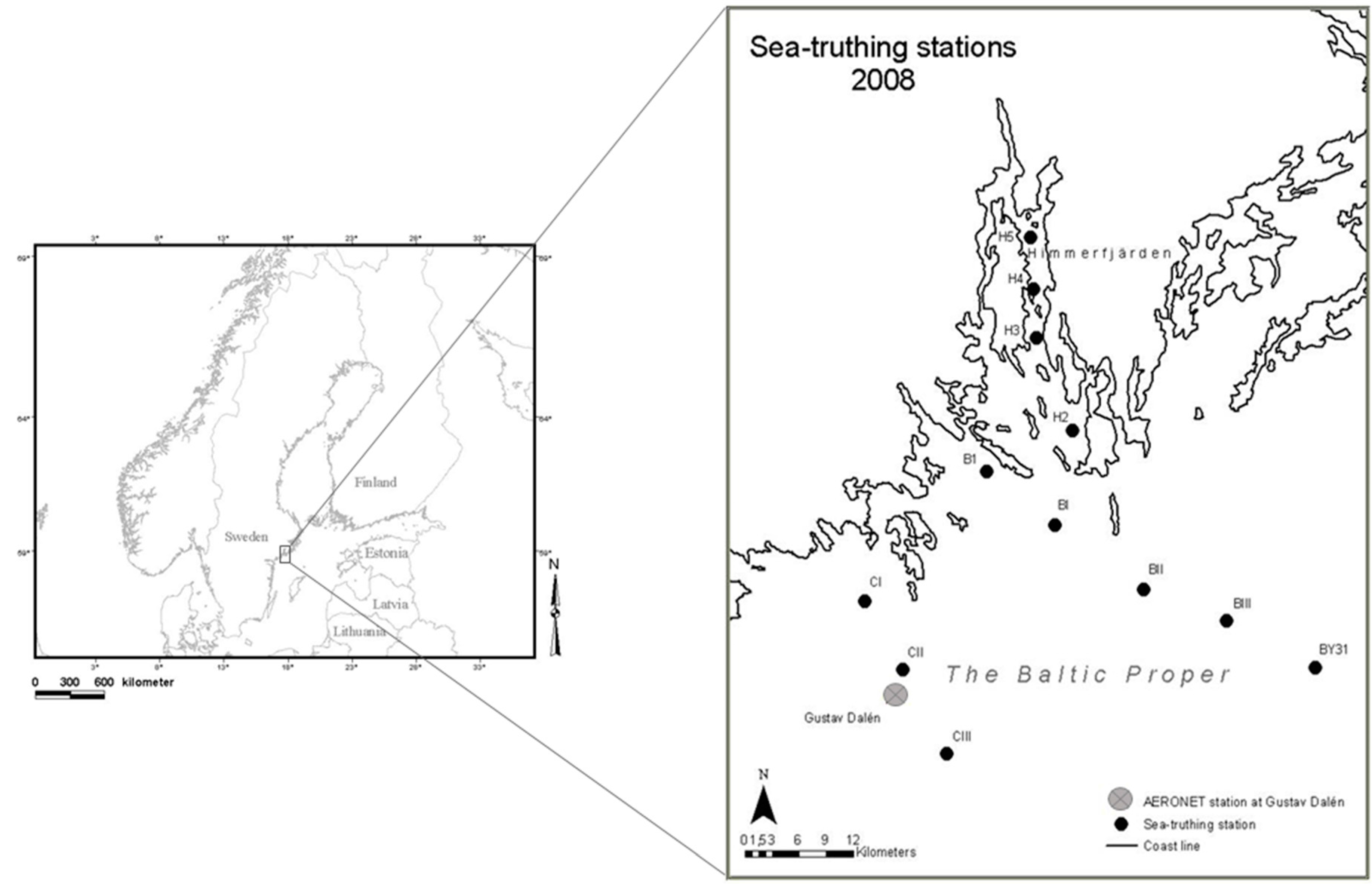
Figure 2.
Geographic distribution of reference data set (RDS), which is a merged data set based on data from the NOMAD and the COLORS projects.
Figure 2.
Geographic distribution of reference data set (RDS), which is a merged data set based on data from the NOMAD and the COLORS projects.
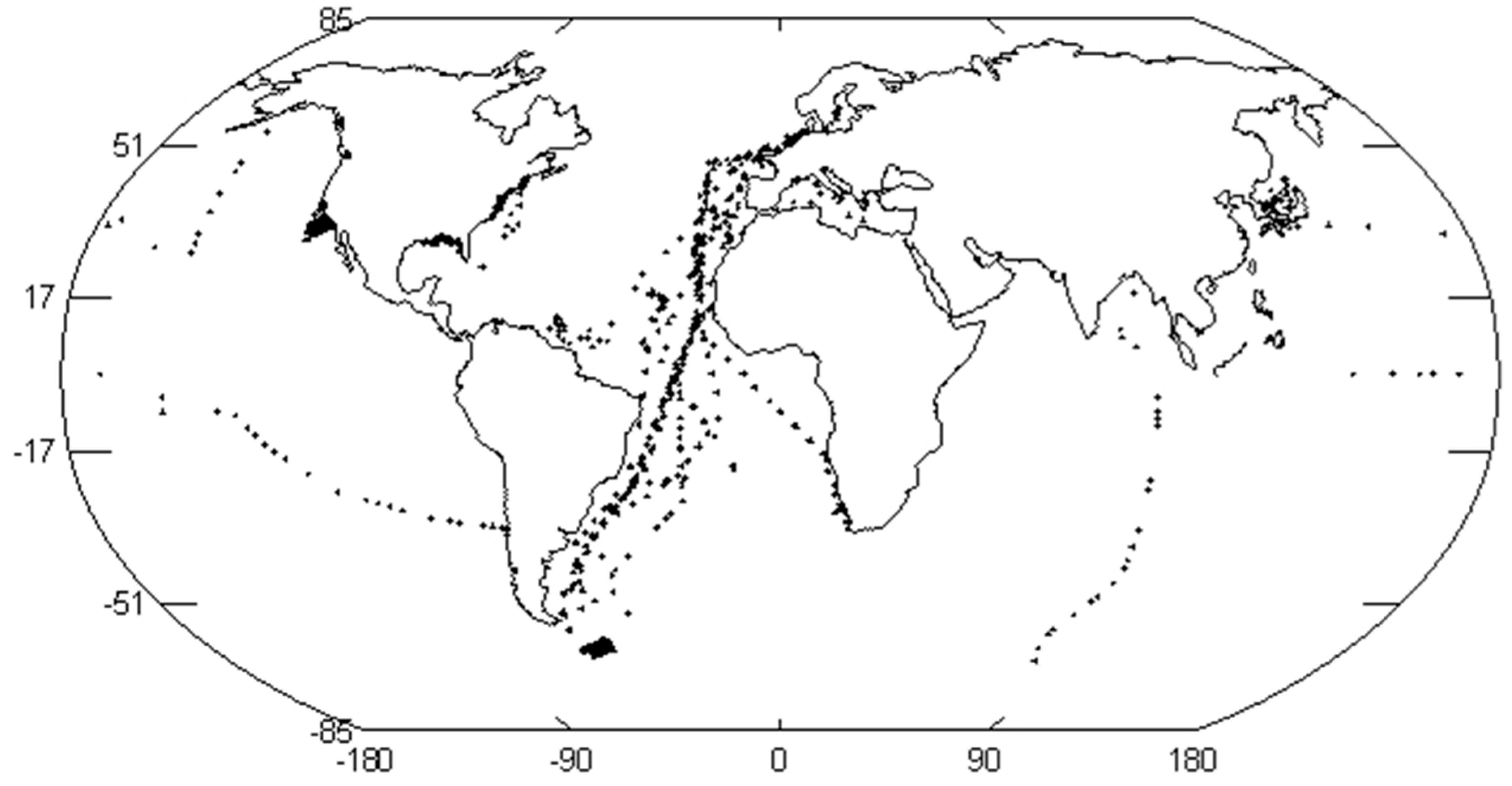
Figure 3.
(a) CDOM absorption, aCDOM at 442 nm vs. SPM concentration; (b) SPM concentration vs. Chl a concentration. The Baltic Sea data set is marked as large black diamonds and plotted along with the reference RDS (small grey diamonds).
Figure 3.
(a) CDOM absorption, aCDOM at 442 nm vs. SPM concentration; (b) SPM concentration vs. Chl a concentration. The Baltic Sea data set is marked as large black diamonds and plotted along with the reference RDS (small grey diamonds).
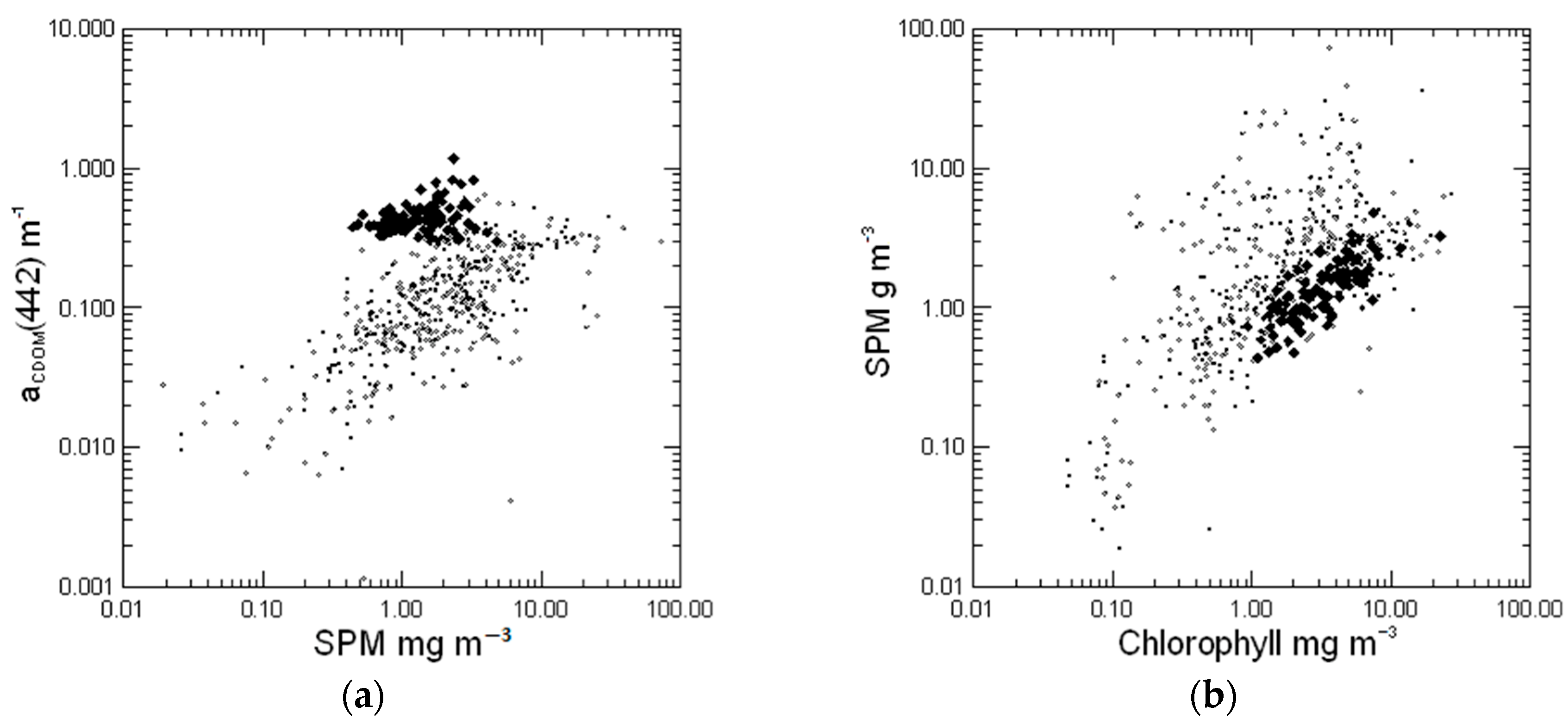
Figure 4.
Ternary plot (a) in the blue (442 nm) and (b) in the red (665 nm) part of the spectrum. The Baltic Sea data set (n = 23) is marked as large black diamonds and plotted along with the RDS (n = 927; small grey diamonds). Note that in the red part of the spectrum (b), the relative phytoplankton absorption (ap/aTot) shows a more similar spread to the one of the reference data set.

Figure 5.
Phytoplankton absorption at 442 nm, ap(442) vs. Chl a concentration. The Baltic Sea data set is marked as larger black diamonds and plotted along with the RDS (small diamonds). The results of ANCOVA showed no significant difference between the two data sets.
Figure 5.
Phytoplankton absorption at 442 nm, ap(442) vs. Chl a concentration. The Baltic Sea data set is marked as larger black diamonds and plotted along with the RDS (small diamonds). The results of ANCOVA showed no significant difference between the two data sets.
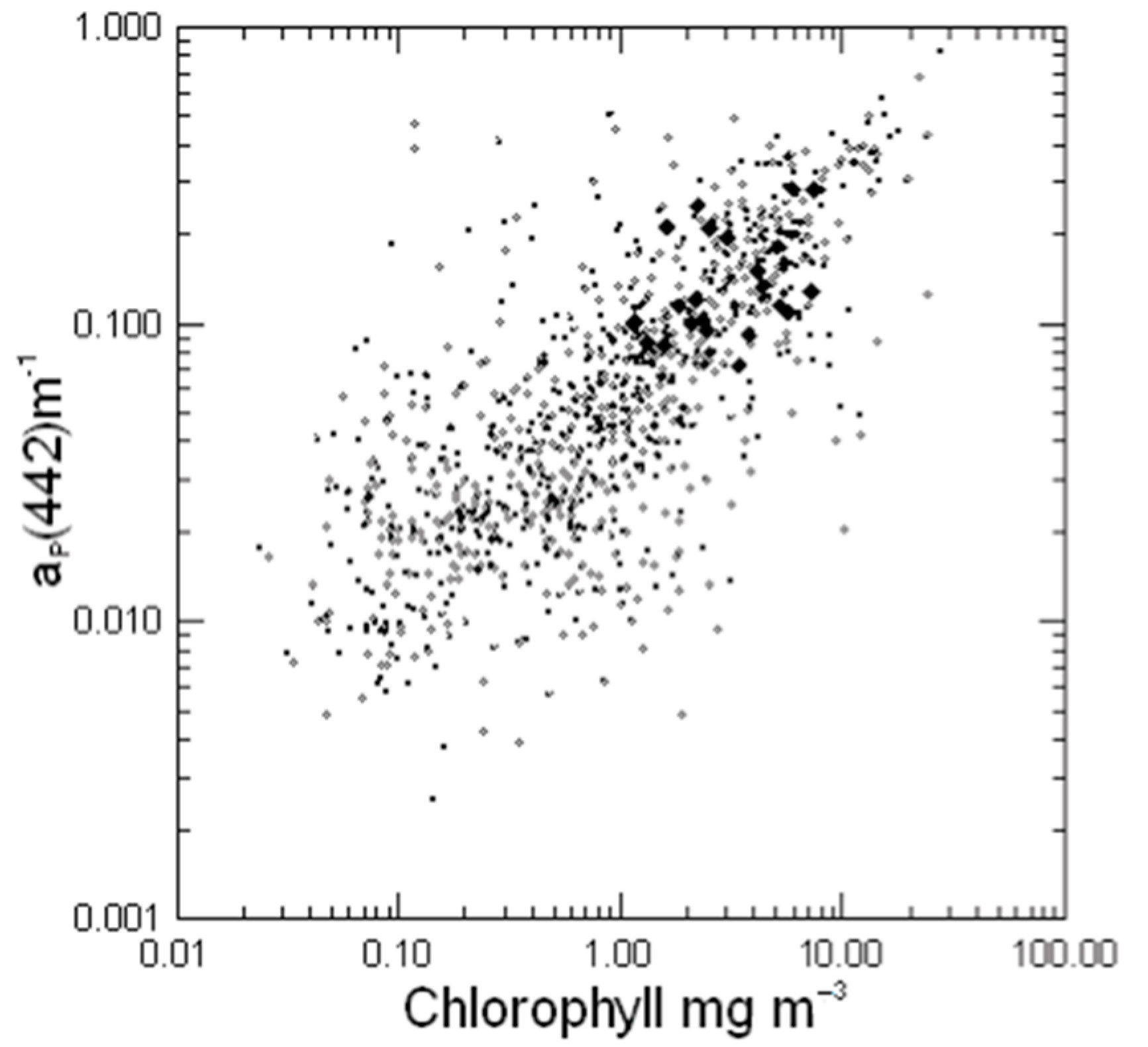
Figure 6.
Non-algal particle absorption, aNAP(442) vs. SPM concentration. The Baltic Sea data set is marked as larger black diamonds and plotted along with the RDS (small diamonds).
Figure 6.
Non-algal particle absorption, aNAP(442) vs. SPM concentration. The Baltic Sea data set is marked as larger black diamonds and plotted along with the RDS (small diamonds).
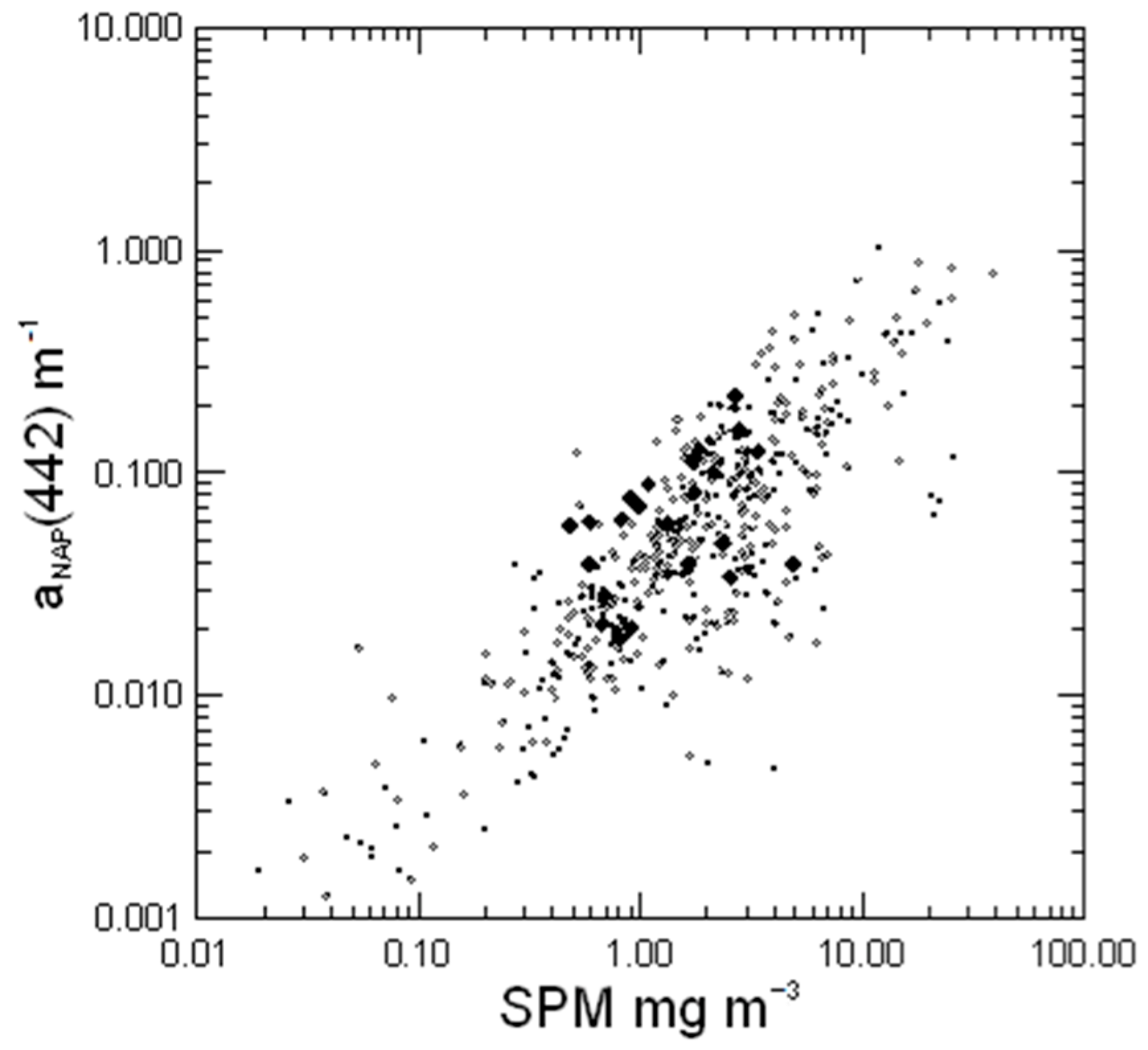
Figure 7.
Histograms of (a) Non-algal absorption slopes; SNAP and (b) CDOM absorption slopes, SCDOM. The Baltic Sea data set is shown as solid line (_____Bal) and plotted along with the RDS (- -Ref).
Figure 7.
Histograms of (a) Non-algal absorption slopes; SNAP and (b) CDOM absorption slopes, SCDOM. The Baltic Sea data set is shown as solid line (_____Bal) and plotted along with the RDS (- -Ref).

Figure 8.
The spectral slope for particle scatter derived from the AC9 data and the corresponding SPM measurements. Note that the Baltic Sea slope (upper slope) differs clearly from the slope of the global data set (lower slope).
Figure 8.
The spectral slope for particle scatter derived from the AC9 data and the corresponding SPM measurements. Note that the Baltic Sea slope (upper slope) differs clearly from the slope of the global data set (lower slope).

Figure 9.
Frequency distribution for (a) backscatter slope () and (b) particle scatter slope (). The Baltic Sea data set is shown as solid line (_____Bal) and plotted along with the RDS (- -Ref).
Figure 9.
Frequency distribution for (a) backscatter slope () and (b) particle scatter slope (). The Baltic Sea data set is shown as solid line (_____Bal) and plotted along with the RDS (- -Ref).
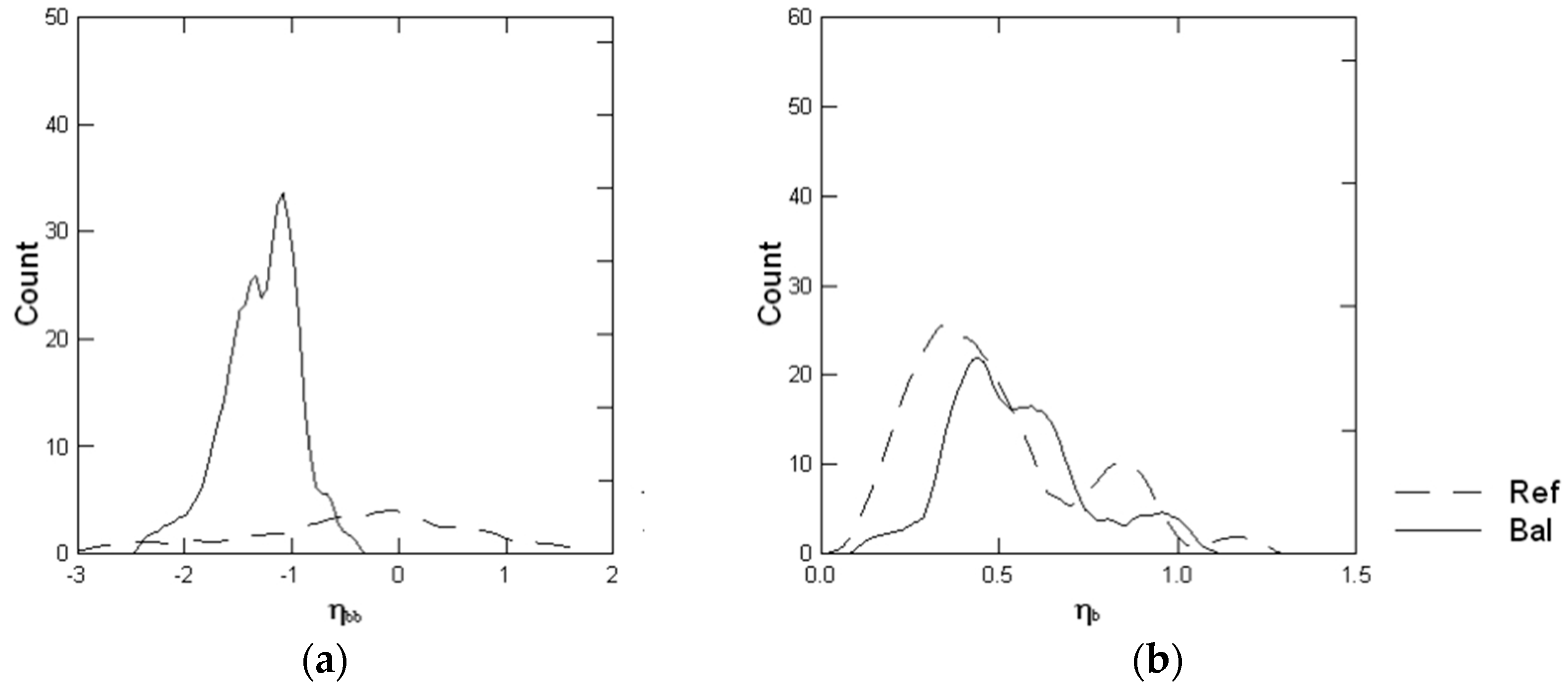
Figure 10.
Frequency distribution for the (β~) for the Baltic and the RDS. The Baltic Sea data set is shown as solid line (_____Bal) and plotted along with the RDS (- -Ref).
Figure 10.
Frequency distribution for the (β~) for the Baltic and the RDS. The Baltic Sea data set is shown as solid line (_____Bal) and plotted along with the RDS (- -Ref).

Figure 11.
Contours of the normalized backscatter coefficient (), plotted against relative refractive index (y-axis) and the Junge Slope (x-axis). Crosses represent measurements at 560 nm and diamonds at 630 nm. The reference line is the relationship given by Mobley et al. [82], and the square is the value for the Petzold phase function [34].
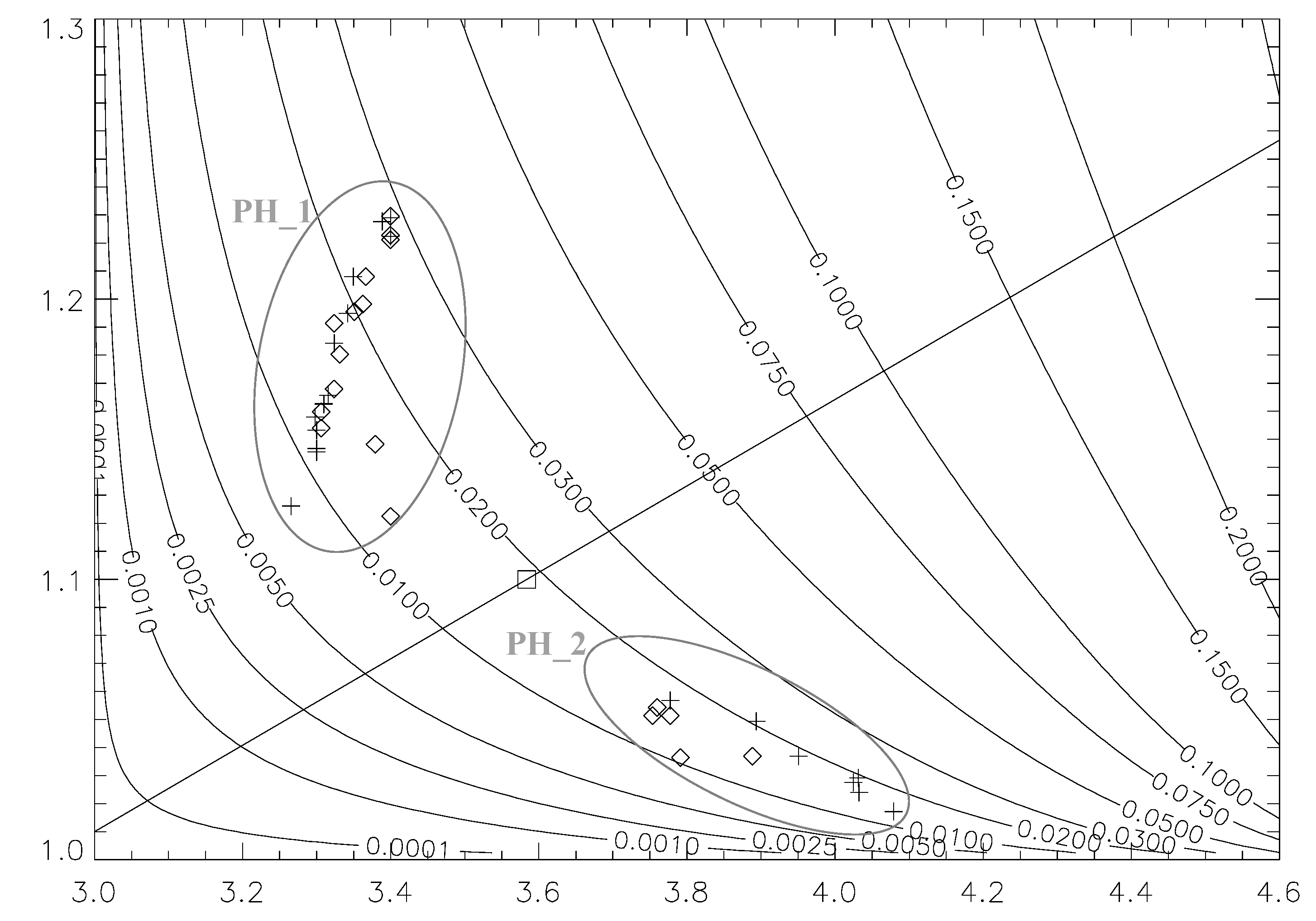
Figure 12.
Phase functions (PF) for the Baltic Sea; phase types compared to the Petzold PF [34]. Both types differ from the Petzold PF; (a) shows the whole PF and (b) shows the PF in backward direction.
Figure 12.
Phase functions (PF) for the Baltic Sea; phase types compared to the Petzold PF [34]. Both types differ from the Petzold PF; (a) shows the whole PF and (b) shows the PF in backward direction.

Figure 13.
The reflectance ratio 490/560 (a) and 560/665 (b) against the Chl a concentration. The Baltic Sea data set (BSDS) is marked as black diamonds.
Figure 13.
The reflectance ratio 490/560 (a) and 560/665 (b) against the Chl a concentration. The Baltic Sea data set (BSDS) is marked as black diamonds.


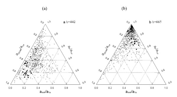
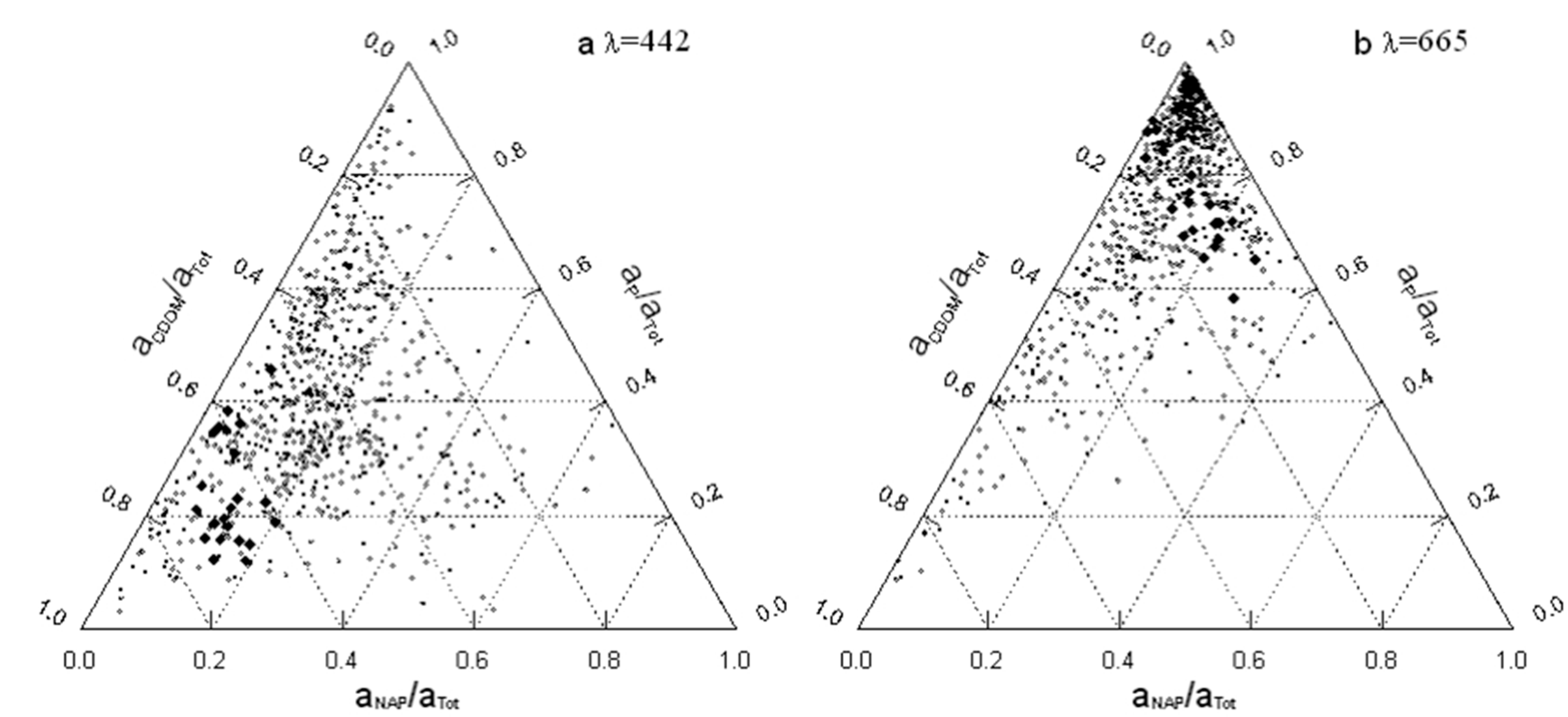
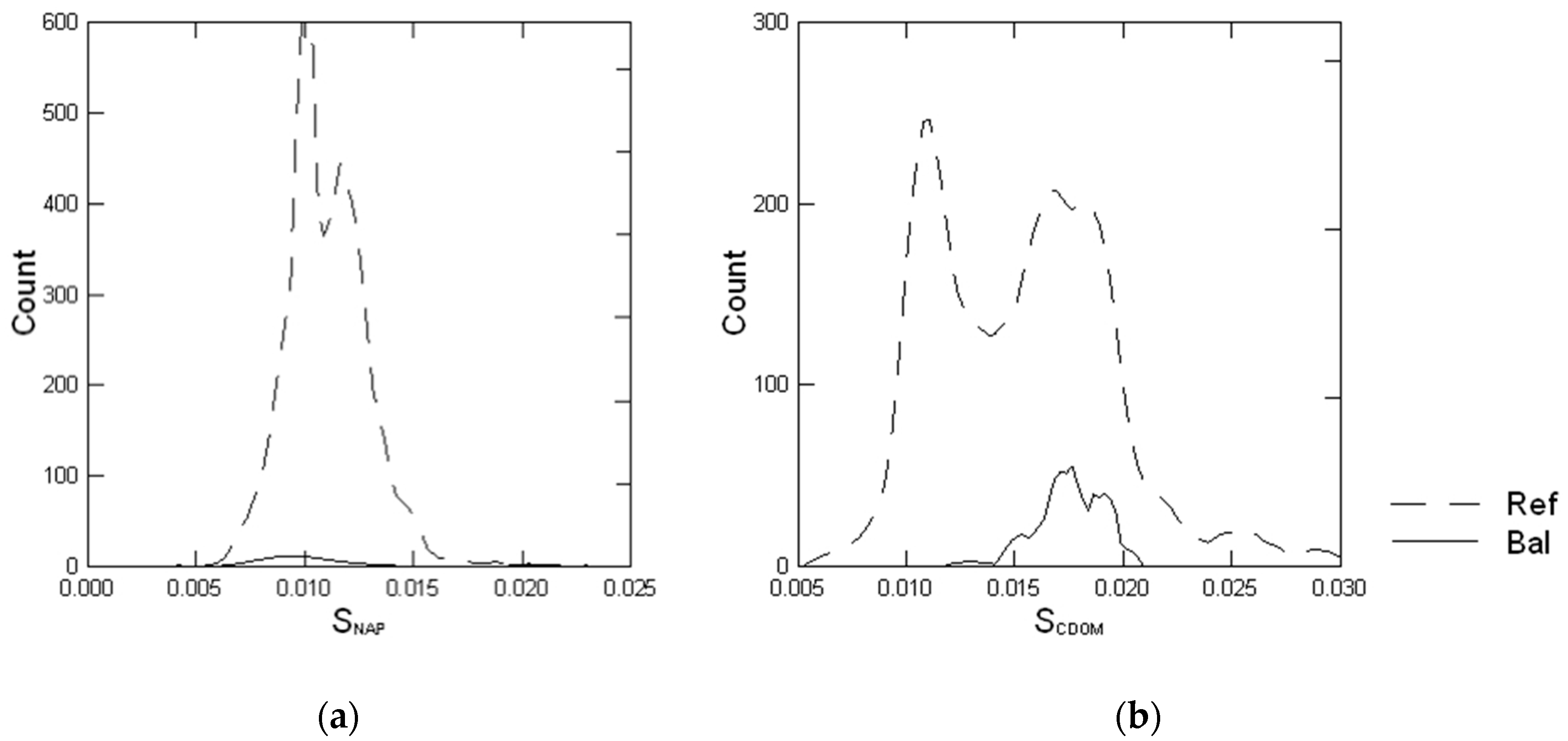
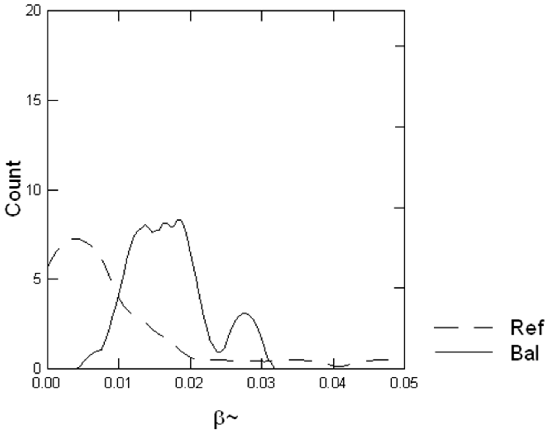
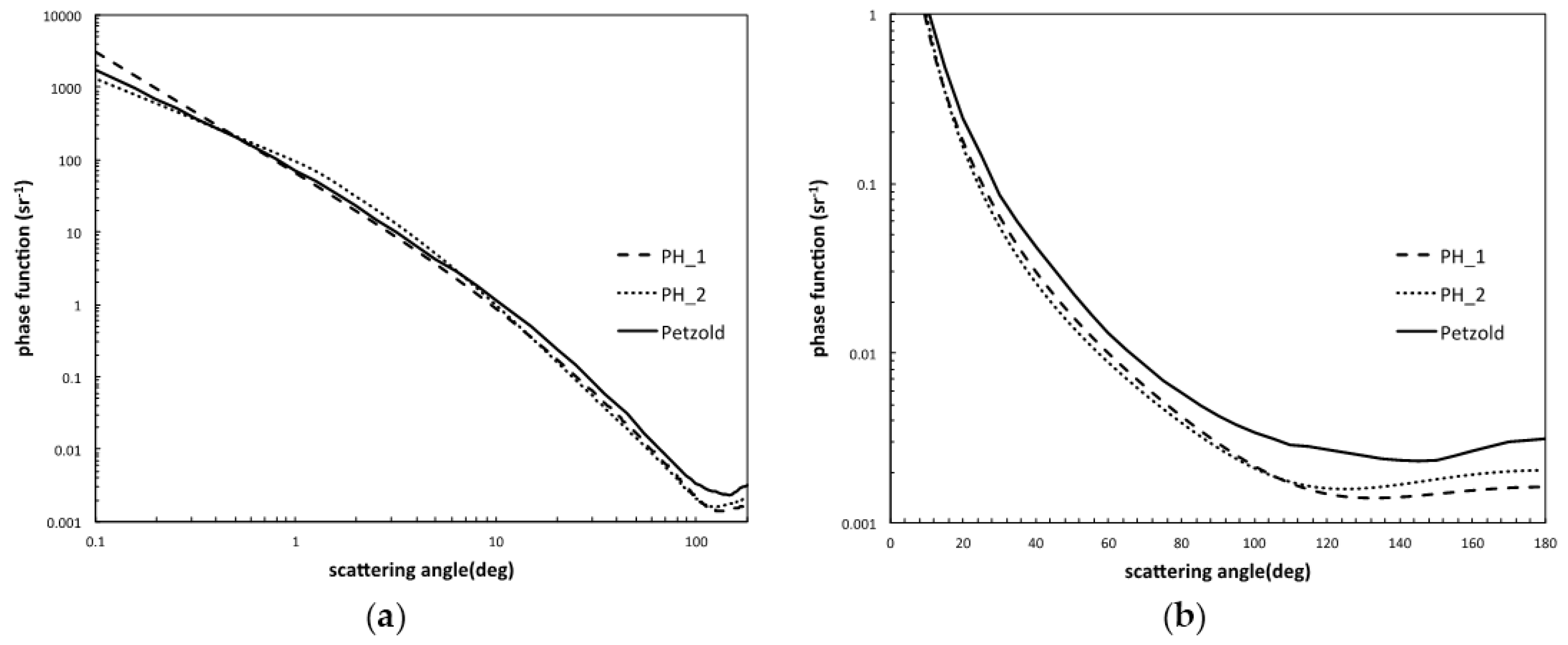
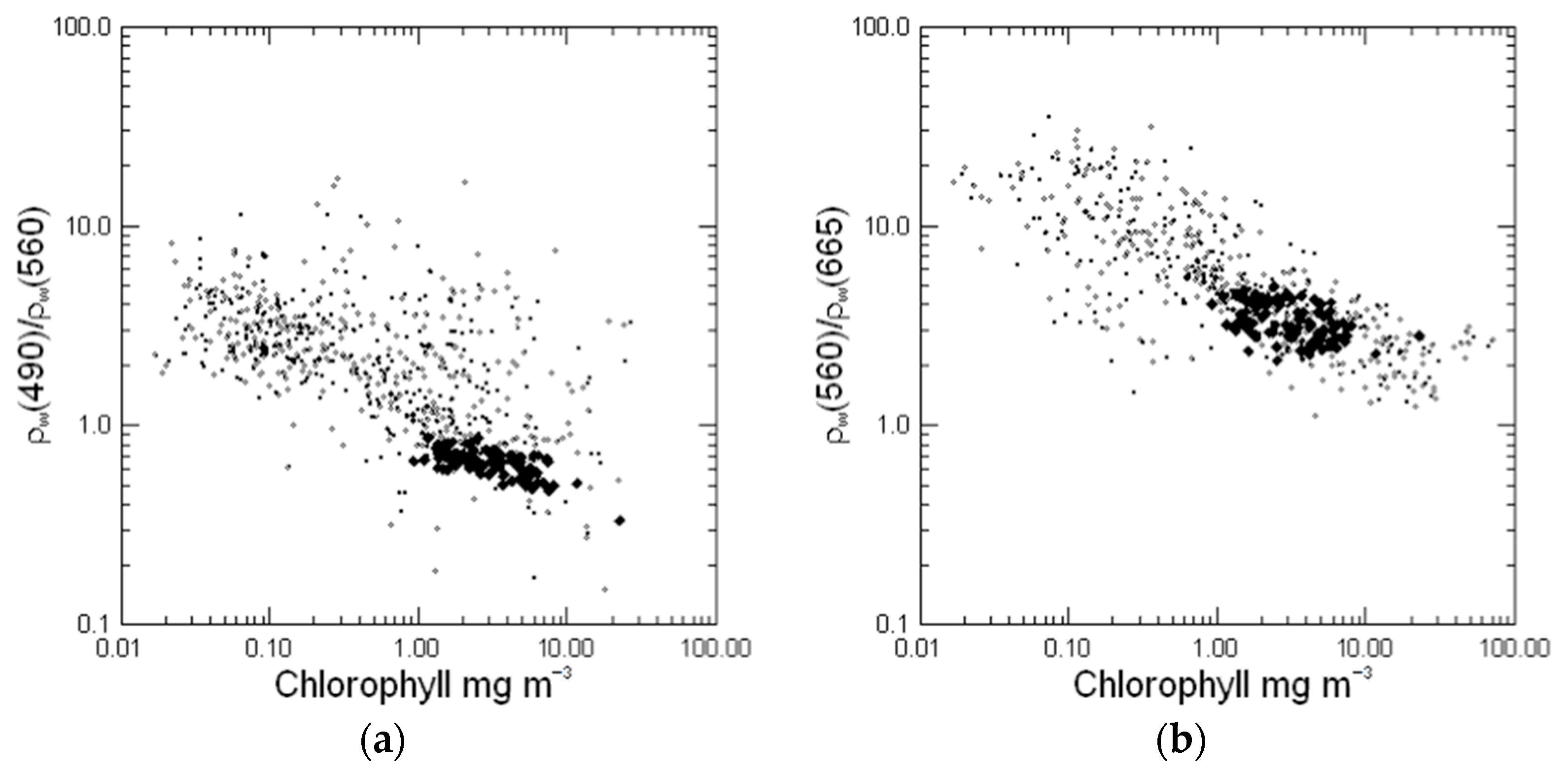
Table 1.
Comparison of the ranges of optical parameters in the Himmerfärden area (NW Baltic Sea) in comparison to other Baltic Sea areas. The table also lists the ranges in Secchi depth (SD). aCDOM refers to CDOM absorption at 440 nm.
Table 1.
Comparison of the ranges of optical parameters in the Himmerfärden area (NW Baltic Sea) in comparison to other Baltic Sea areas. The table also lists the ranges in Secchi depth (SD). aCDOM refers to CDOM absorption at 440 nm.
| Baltic Sea Area | [Chl a] | [SPM] | aCDOM | SD | References |
|---|---|---|---|---|---|
| µg L−1 | g m−3 | m−1 | m | ||
| Arkona Sea | 0.3–7.0 | 0.7–9.0 | 0.2–0.4 | 5.0–9.5 | [9,10] |
| Bornholm Sea | 0.4–4.0 | 0.4–5.0 | 0.2–0.3 | 2.0–10.5 | [9] |
| Gotland Sea | 0.2–4.0 | 3.0–6.0 | 0.2–0.4 | 3.0–10.0 | [9] |
| Pomeranian Bight, Germany | 0.4–13.0 | 0.5–20.0 | 0.2–0.9 | 3.0–7.0 | [9,11,12] |
| Gulf of Gdansk Poland | 0.4–72.6 | 0.4–15.7 | 0.4–4.4 | 4.5–7.0 | [11,12,13] |
| SE Baltic Sea, Lithuanian coast | 0.6–116.2 | 1.1–32.0 | 0.01–2.0 | 4.0–6.0 | [12,14] |
| Pärnu Bay, Estonia | 0.7–10.7 | 5.0–24.3 | 0.6–3.7 | 0.5–4.3 | [15,16] |
| Gulf of Riga, Estonia | 2.0–46.0 | 10.0–24.0 | 1.5–13.0 | 3.1–6.9 | [10,17,18] |
| Gulf of Finland | 1.2–130 | 0.8–20.0 | 0.6–1.2 | 1.8–4.0 | [19,20] |
| NW Baltic proper | 0.4–52.4 | 0.5–21.7 | 0.3–4.1 | 0.7–12.8 | [4,8] |
| Öre Estuary, Bothnian Sea, SE | 0.5–96.4 | 0.2–20.9 | 0.75–8.8 | 0.5–6.0 | [8] |
Table 2.
Ranges of optical parameters in the Himmerfjärden area (Baltic Sea) with median, upper quartile (UQ) and lower quartile (LQ) as well as number of observations (n). aCDOM refers to CDOM absorption at 440 nm.
Table 2.
Ranges of optical parameters in the Himmerfjärden area (Baltic Sea) with median, upper quartile (UQ) and lower quartile (LQ) as well as number of observations (n). aCDOM refers to CDOM absorption at 440 nm.
| Data Set | Optical Property | Unit | Range | Median | LQ | UQ | n |
|---|---|---|---|---|---|---|---|
| Baltic Sea | [Chl a] | µg L−1 | 0.9–22.5 | 3.1 | 2.0 | 4.8 | 97 |
| [SPM] | g m−3 | 0.4–4.8 | 1.3 | 0.9 | 1.8 | 97 | |
| aCDOM | m−1 | 0.3–1.2 | 0.42 | 0.38 | 0.49 | 98 | |
| Global RDS | [Chl a] | µg L−1 | 0.02–70.2 | 0.7 | 0.2 | 2.4 | 1982 |
| [SPM] | g m−3 | 0.01–81.2 | 1.9 | 0.8 | 3.8 | 556 | |
| aCDOM | m−1 | 0.001–0.6 | 0.06 | 0.03 | 0.14 | 860 |
RDS: reference data set.
© 2018 by the authors. Licensee MDPI, Basel, Switzerland. This article is an open access article distributed under the terms and conditions of the Creative Commons Attribution (CC BY) license (http://creativecommons.org/licenses/by/4.0/).
Share and Cite
MDPI and ACS Style
Kratzer, S.; Moore, G. Inherent Optical Properties of the Baltic Sea in Comparison to Other Seas and Oceans. Remote Sens. 2018, 10, 418. https://doi.org/10.3390/rs10030418
AMA Style
Kratzer S, Moore G. Inherent Optical Properties of the Baltic Sea in Comparison to Other Seas and Oceans. Remote Sensing. 2018; 10(3):418. https://doi.org/10.3390/rs10030418
Chicago/Turabian StyleKratzer, Susanne, and Gerald Moore. 2018. "Inherent Optical Properties of the Baltic Sea in Comparison to Other Seas and Oceans" Remote Sensing 10, no. 3: 418. https://doi.org/10.3390/rs10030418
Note that from the first issue of 2016, this journal uses article numbers instead of page numbers. See further details here.