Evaluation of the Ability of Spectral Indices of Hydrocarbons and Seawater for Identifying Oil Slicks Utilizing Hyperspectral Images

Abstract

It is important to detect floating oil slicks after spill accidents, and hyperspectral remote sensing technology is capable of achieving this task. Traditional methods mainly utilize the spectral indices of hydrocarbons to detect floating oil slicks, but are poor at distinguishing the thickness of oil slicks and cannot detect sheens. Since the spectra of oil slicks should be affected by seawater as well as oil, this paper investigated the use of spectral indices of hydrocarbons and seawater to identify different thicknesses of oil slicks. In this research, a measurement, called index separability (IS), was proposed for quantitatively evaluating the identification ability of these spectral indices. Based on the evaluation results, experiments were conducted to validate the applicability of these spectral indices. The results show that the spectral indices of hydrocarbons are more suitable for detecting continuous true color oil slicks and emulsions and that spectral indices of seawater are more suitable for sheens and seawater. In addition, the spectral indices of hydrocarbons and seawater are complementary for detecting oil slicks. Finally, combining the spectral indices of hydrocarbons and seawater is conducive to achieving more accurate oil slick recognition results.

1. Introduction

A large amount of oil is rapidly leaked in an oil spill accident. Oil slicks created by an accident float on the sea surface and seriously damage the marine environment [1,2,3,4,5]. Mapping oil spills is vital for evaluating the damage and making decisions to avoid secondary disasters. Hyperspectral remote sensing imaging involves hundreds of bands whose wavelengths range from visible to shortwave infrared, which allows for precise mapping of the oil spills [6,7,8]. However, restricted by sun-glint and the weakness of spectral signals of sheens [9], traditional hyperspectral oil spill mapping methods mainly focus on detecting true color oil slicks and emulsions, and the surrounding sheens are not detected by the oil spill mapping products.

In 2010, the Gulf of Mexico (GoM) oil spill was monitored by the Airborne Visible Infrared Imaging Spectrometer (AVIRIS). Numerous studies were proposed based on hyperspectral images captured in that accident. Clark et al. [6] mapped oil slicks through the near-infrared absorption spectral characteristics of hydrocarbons. In the results, different water-to-oil ratios and thicknesses of oil slicks were identified accurately, but only true color oil slicks were included in the results. The least contaminated seawater or sheens around the true color oil slicks and emulsions were not detected by this method. Alam and Sidike proposed a method to detect oil slicks using dimensionality reduction and target detection with hyperspectral image data [10]. Although the method gave excellent detection results for continuous and discontinuous true color oil slicks, it could not distinguish different thicknesses of oil slicks nor identify sheens. An oil slope index (OSI) was put forward by Li et al. [11] for detecting oil slicks, but only emulsions were detected via this method. Liu et al. [12] used density-based clustering to select a specific spectral signature from a hyperspectral image for oil spill detection, but again, only emulsions were detected in the results. Traditional hyperspectral oil-slick identification methods focus on detecting thick oil slicks because they contain abundant hydrocarbons, whereas sheens contain much less. Thus, thick oil slicks show greater hydrocarbon spectral characteristics than the surrounding sheens [13,14]. The spectral curves of sheens are very similar to that of seawater. Thus, using traditional methods, it is difficult to differentiate sheens from seawater using the spectral indices of hydrocarbon substances.

The purpose of this research is to find new ways to identify different thicknesses of oil slicks, including sheens or less contaminated seawater. The basis of this research is that oil slicks on the sea surface are somewhat influenced by seawater. The transparency of thick oil slicks is weak [15,16,17,18], and their spectra are weakly influenced by seawater. However, sheens are nearly translucent, so the spectra of sheens are greatly influenced by seawater. Thus, this paper proposes a hypothesis: the spectral indices of hydrocarbons and seawater can be used together to identify oil slicks with different thicknesses. Based on this hypothesis, a measurement called the index separability (IS) was proposed to quantitatively evaluate the feasibility of using spectral characteristics to identify oil slicks of different thicknesses. An oil slick identification method was established according to the evaluation results.

AVIRIS hyperspectral images captured at the Deep Water Horizon (DWH) oil spill accident in GoM 2010 [19] were used to conduct experiments to validate the hypothesis and the proposed IS measurement. Details of the methods, experiments, and conclusions are provided in Section 2, Section 3, Section 4 and Section 5.

2. Materials and Methods

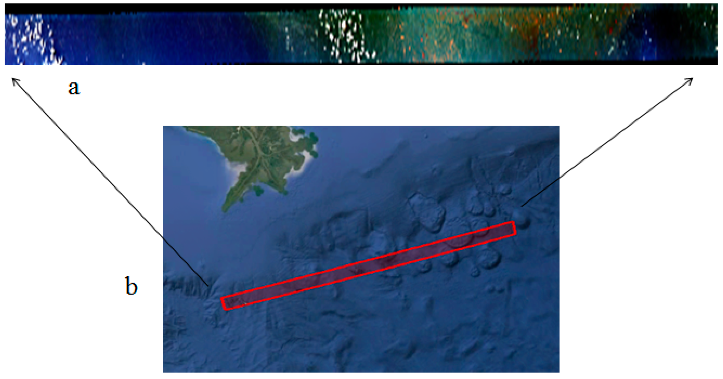
2.1. Study Area

During the DWH oil spill in 2010, a large amount of crude oil leaked into the GoM. Many high-quality aerial hyperspectral images were collected to monitor the oil spill pollution. These images have been used in numerous studies of oil spills, because this oil spill was typical and the images are of high quality [6,7,10,12,16]. The experimental hyperspectral image adopted in this paper is one of the collected images. The experimental data were obtained via an AVIRIS imager with a spatial resolution of 7.6 m on 17 May 2010. The flight name of the data, on the official website, is f100517t01p00r11. The image has 19,736 lines and 886 samples, and every pixel has 192 bands after removal of some noise bands. The wavelengths of the pixels range from 365.9 nm to 2466.5 nm. The scope of the image latitude and longitude are 28.428239°N to 28.853579°N and 87.964761°W to 89.459463°W, respectively. The scale of the original image is too large to be shown clearly here, so the thumbnail of the experimental data and the scope of the study area are displayed in Figure 1.

The original image data are over 10 GB in size and too large for the software to process. Thus, three training areas, shown in Figure 2, were extracted from the study area to validate the hypotheses received from the training results. Training image (a) contains emulsions and sheens; it is appropriate for evaluating the applicability of the spectral indices for identifying thicker oil slicks. Training image (b) is the boundary of the oil spill. It can be used to evaluate the applicability of the spectral indices to identify sheens and seawater. Training image (c) consists of different thicknesses of oil slicks, and can be used to assess the ability of the spectral indices to differentiate diverse thicknesses of oil slicks. In addition to these test images, three test areas of the study area were extracted to explore the performance of the oil slick identification model established by the evaluation results. The test areas are shown in Figure 3. They are portions of the original image captured along the airline, so there are black borders in the test areas. To validate the hypothesis correctly, the training areas are not portions of the test areas.

2.2. Data Preprocessing

Atmospheric correction is an important preprocessing step for remote-sensing data. The original experimental data were processed through fast line-of-sight atmospheric analysis of a spectral hypercubes (FLAASH) model using ENVI. For the correction process, the atmospheric model was tropical, the aerosol model was maritime, and the atmospheric correction result showed an average water amount of 3.8067 cm. During the investigation, software for training, testing, and oil spill mapping was programmed using visual C++.

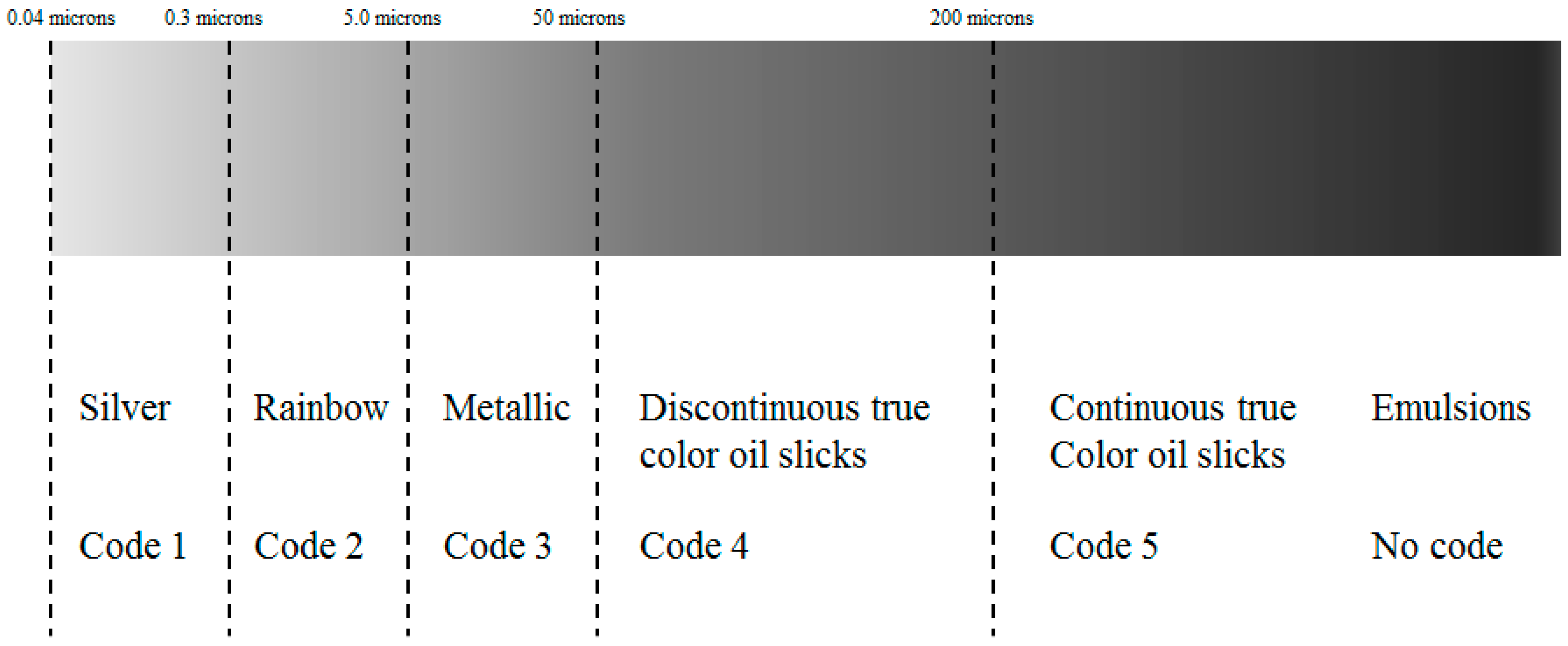
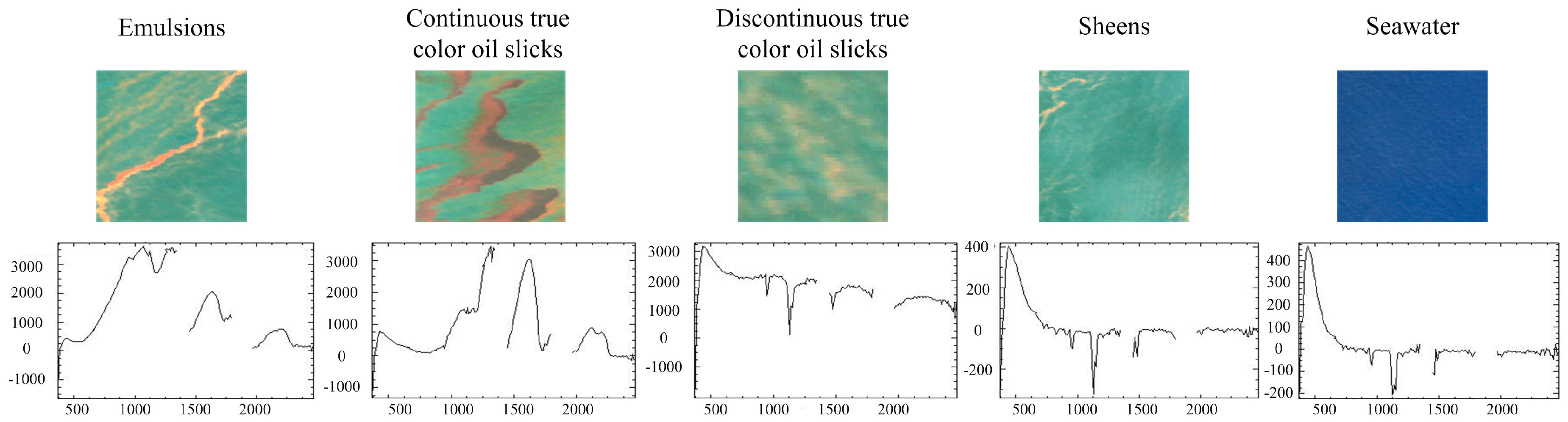
2.3. Oil Slick Properties

In 2004, the useful Bonn Agreement Oil Appearance Code was adopted as a standard method to assess the volume of oil on water. According to the handbook, the oil slick thickness is coded from 1–5 for sheens (silver/gray), rainbow, metallic, discontinuous true oil color, and continuous true oil color (

Table 1. Two methods to code oil slick thickness.

Thickness	Code	Bonn Agreement Oil Appearance Code	Open Water Oil Identification Job Aid
Thinner	1	Sheen (silver/gray)	Silver
	2	Rainbow	Rainbow
	3	Metallic	Metallic
	4	Discontinuous true oil color	Transitional dark
	5	Continuous true oil color	Dark
Thicker	No code	Emulsion	Emulsion

). The code should not be used to quantify areas of emulsion [20]. In 2016, NOAA and the U.S. Coast Guard released the Open Water Oil Identification Job Aid (OWOIJA) to describe oil slicks (Table 1). This Job Aid is designed to describe oil slicks. There is little difference between these two ways of describing oil slick thickness. This paper adopts the Bonn Agreement Oil Appearance Code to describe the oil slicks. Because thin oil slicks evaporate quickly [21,22,23,24], it is hard to observe or detect silver, rainbow, and metallic respectively in the experimental image, which is captured weeks after the oil spill accident. Thus, silver, rainbow, and metallic are collectively referred to as sheens. In this research, the thickness of oil slicks is classified from the thinnest to the thickest into four types: sheens (code 1–3), discontinuous true color oil (code 4), continuous true color oil (code 5), and emulsion (E). The thickness classification is showed in Figure 4.

After atmospheric correction, training samples of seawater and different thicknesses of oil slicks were selected according to the oil film properties proposed and proven in former studies. The color of sheens varied from almost transparent to silver/gray, rainbow and metallic. There is a high reflectance in the ultraviolet bands for the sheens [8,16], which is mainly formed through the diffusion of thicker oils, so that sheens always surround thicker oils [20]. Discontinuous true color oil slicks look orange; some thin oil slicks of code 4 appear patchy. Discontinuous true color oil slicks of 50–150 microns have a lower temperature than seawater, while those thicker than 150 microns have a higher temperature. Continuous true color oil slicks appear continuous and represent the true color of crude oil: dark brown or black. Because the thickness of continuous true color oil slick is over 200 microns, they have a higher absorption of solar heat input and distinct reflectance signals in the infrared bands [16]. Emulsions are water-to-oil mixtures that appear orange, brown, and/or red. The thickness of emulsions exceeds that of true color oil slicks, but it is difficult to accurately describe an emulsion’s thickness, and thus, the Bonn agreement and OWOIJA do not encode emulsions. Emulsions are distributed in the convergence zones, which are narrow long bands of oils [24]. Since the thickness of emulsions exceeds 500 microns, they have a high reflectance in the infrared bands [6]. The typical color, shape, and spectral characteristics of oil slicks are listed above. Figure 5 shows the photos and spectra of seawater and oil slicks of different thicknesses.

2.4. Spectral Indices of Hydrocarbons and Seawater

A variety of spectral indices can be used to describe oil slicks and seawater. This paper used several spectral indices to monitor floating oil slicks and seawater compositions (

Table 2. The spectral indices involved in this study.

Representation	Characteristic	Formula	Reference
Hydrocarbons	Fluorescence Index, FI	$\mathrm{FI}=\frac{{\mathrm{R}}_{\mathrm{B}}-{\mathrm{R}}_{\mathrm{R}}}{{\mathrm{R}}_{\mathrm{B}}+{\mathrm{R}}_{\mathrm{R}}}$	[25]
Hydrocarbons	Rotation-Absorption Index, RAI	$\mathrm{RAI}=\frac{{\mathrm{R}}_{\mathrm{B}}-{\mathrm{R}}_{\mathrm{IR}}}{{\mathrm{R}}_{\mathrm{B}}+{\mathrm{R}}_{\mathrm{IR}}}\sqrt{{\displaystyle \sum }{\mathrm{b}}_{\mathrm{i}}^2}$	[25]
Hydrocarbons	Hydrocarbon Index, HI	$\mathrm{HI}=\left({\mathsf{\lambda }}_{\mathrm{B}}-{\mathsf{\lambda }}_{\mathrm{A}}\right)\frac{{\mathrm{R}}_{\mathrm{C}}-{\mathrm{R}}_{\mathrm{A}}}{{\mathsf{\lambda }}_{\mathrm{C}}-{\mathsf{\lambda }}_{\mathrm{A}}}+{\mathrm{R}}_{\mathrm{A}}-{\mathrm{R}}_{\mathrm{B}}$	[26]
Hydrocarbons	Reflectance of Green, RG	$\mathrm{RG}=\max \left({\mathrm{R}}_{\mathrm{Green}}\right)$	[27]
Hydrocarbons	Reflectance of Red, RR	$\mathrm{RR}=\min \left({\mathrm{R}}_{\mathrm{Red}}\right)$	[27]
Seawater	Water Absorption Feature, WAF	$\mathrm{WAF}=\frac{{\mathrm{R}}_{\mathrm{A}}+{\mathrm{R}}_{\mathrm{C}}}{2}-{\mathrm{R}}_{\mathrm{B}}$	[28]
Seawater	Chlorophyll, CHL	$\begin{array}{c}\mathrm{CHL}={10}^{\mathrm{y}}\mathrm{y}={\mathrm{a}}_0+{\mathrm{a}}_1\mathrm{x}+{\mathrm{a}}_2{\mathrm{x}}^2+{\mathrm{a}}_3{\mathrm{x}}^3+{\mathrm{a}}_4{\mathrm{x}}^4\mathrm{x}\\ \hspace{1em}\hspace{1em}\hspace{1em}\hspace{1em}\hspace{1em}\hspace{1em}\hspace{1em}\hspace{1em}=\log (\frac{\max ({\mathrm{R}}_{433,490,510})}{{\mathrm{R}}_{555}})\end{array}$	[29]
Seawater	Colored Dissolved Organic Matter, CDOM	$\mathrm{CDOM}=5.2{\mathrm{x}}^{-2.76}\mathrm{x}=\frac{{\mathrm{R}}_{565}}{{\mathrm{R}}_{660}}$	[30]

). Although some methods are based on empirical methods that are critical for the parameters, they can qualitatively assess oil slicks and seawater.

The fluorescence index (FI) and the rotation absorption index (RAI) exhibit the fluorescence characteristics of oil slicks [25]. They highlight the fluorescence behavior of surface oil slicks and the increased red reflectance of surface oil. Loos used these indices to detect oil slicks in the GoM accident based on multispectral images. For the experimental AVIRIS data, $R_B$, $R_R$, and $R_{IR}$ are the reflectance values for the hyperspectral data at 433 nm, 648 nm, 889 nm, respectively, and $b_i$ is the reflectance of band i. The FI and RAI are practical indices for oil slick detection, so they are utilized in research to describe the spectral characteristics of hydrocarbons in oil slicks. It has been shown that the spectral response, an absorption feature at 1600 nm and 1800 nm, is caused by the overtone absorption of carbon-hydrogen bonds and can be used to identify oil slicks. Using this feature, Kühn et al. [26] proposed the Hydrocarbon Index (HI), which comprises the hydrocarbons absorption features at 1730 nm to identify substances containing hydrocarbons. For the formula of HI, $R_A$, $R_B$, and $R_C$ are the reflectance values to the left of 1730 nm, at 1730 nm, and to the right of 1730 nm, respectively, and λ is the wavelength. For the AVIRIS data, the λ of A, B, and C are 1721 nm, 1731 nm, and 1741 nm, respectively. The value of HI is higher if a detected site contains hydrocarbon substances. Sun et al. (2013) suggested that the spectral signals in green and red bands are related to the thickness of oil slicks [27], and thus, this paper used $R_G$ to represent the oil slick spectral characteristics in the green bands and 𝑅𝑅 to represent the oil slick spectral characteristics in the red bands. For the experimental data in this research, the wavelength ranges of green and red bands were 511–579 nm and 618–714 nm, respectively. This research used these two spectral features of oil slicks because they are spectral characteristics in the visible bands and have been proven to be useful.

In addition to hydrocarbon substances, seawater should also influence the spectra of oil slicks. This research investigated several spectral indices of seawater composition to determine how to identify oil slicks using the spectral indices of seawater. The Water Absorption Feature (WAF) is the absorption feature of water caused by H-O at 1440 nm [28]. It has been validated as correct and sensitive for water detection. In the equation, $R_A$, $R_B$, and $R_C$ are the reflectance values at 1343 nm, 1453 nm, and 1563 nm of the hyperspectral data, respectively. Models evaluating chlorophyll (CHL) and Colored Dissolved Organic Matter (CDOM) are involved in this research because CHL and CDOM are important components of seawater. They can be used to demonstrate how to detect oil slicks using the spectral indices of seawater. Although the models evaluating CHL and CDOM concentrations are empirical and may not be suitable for the studied sea area, they can qualitatively assess the concentrations of seawater composition. In this research, CHL is calculated using the classical OC4 model. In this paper, the values of $a_0$, $a_1$, $a_2$, $a_3$, and $a_4$ refer to the paper by Hu et al. [29]: 0.3272, −2.9940, 2.7218, −1.2259, and −0.5683, respectively. CDOM is calculated using the method proposed by Kutser et al. [30,31]. Since AVIRIS data do not have bands of 565 nm and 660 nm, $R_{565}$ was replaced by the average of $R_{560}$ and $R_{570}$, and $R_{660}$ was replaced by the average of $R_{656}$ and $R_{666}$.

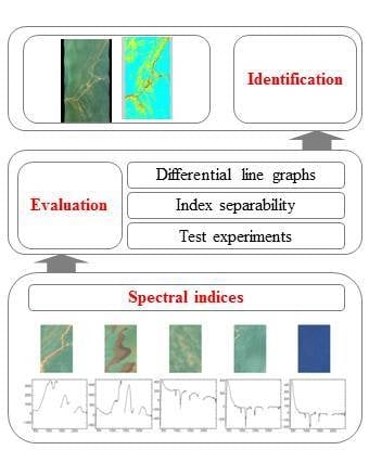
2.5. Evaluation Measurement

Eight spectral indices are studied in this paper. According to the original hypothesis, different indices might possess different abilities to identify different thickness of oil slicks. For example, the spectral indices of hydrocarbons might be more sensitive for thicker oil slicks but may not be able to distinguish between sheens and seawater. To assess spectral indices quantitatively, the IS measurement was proposed in this paper. The main idea of the IS measurement is to evaluate a spectral index’s applicability to identify oil slicks by calculating the interclass distance of training samples.

$$I{S}_{i,j}^I=\frac{MinI{D}_{i,j}^I}{AvgI{D}^I}$$

(1)

$$AvgI{D}^I=\frac{\max (MaxI{D}_{i,j}^I)}{4}$$

(2)

The calculation of IS is based on the spectral index distance (ID) of the training samples. I is a member of the spectral indices in Table 2, and i and j are elements of {seawater, code 1–3, code 4, code 5, and emulsions}. MinID is the minimum ID of the training results between i and j. MaxID is the maximum ID of the training results between i and j. AvgID is the average gap of I for training samples i and j. Since five elements are discussed for the research, the gap is a quarter of maximum gap. IS is similar to the concept of interclass distance between two classes in statistics. The measurement of IS is constructed to evaluate an index’s ability to distinguish diverse thicknesses of oil slicks via the distances between the training results. A larger IS indicates a stronger ability to identify the thickness of oil slick.

The IS measurement was proposed to evaluate the spectral indices, but it was not the only method of evaluation used. During the experiments, the abilities of the spectral indices to identify oil slicks were evaluated in three ways:

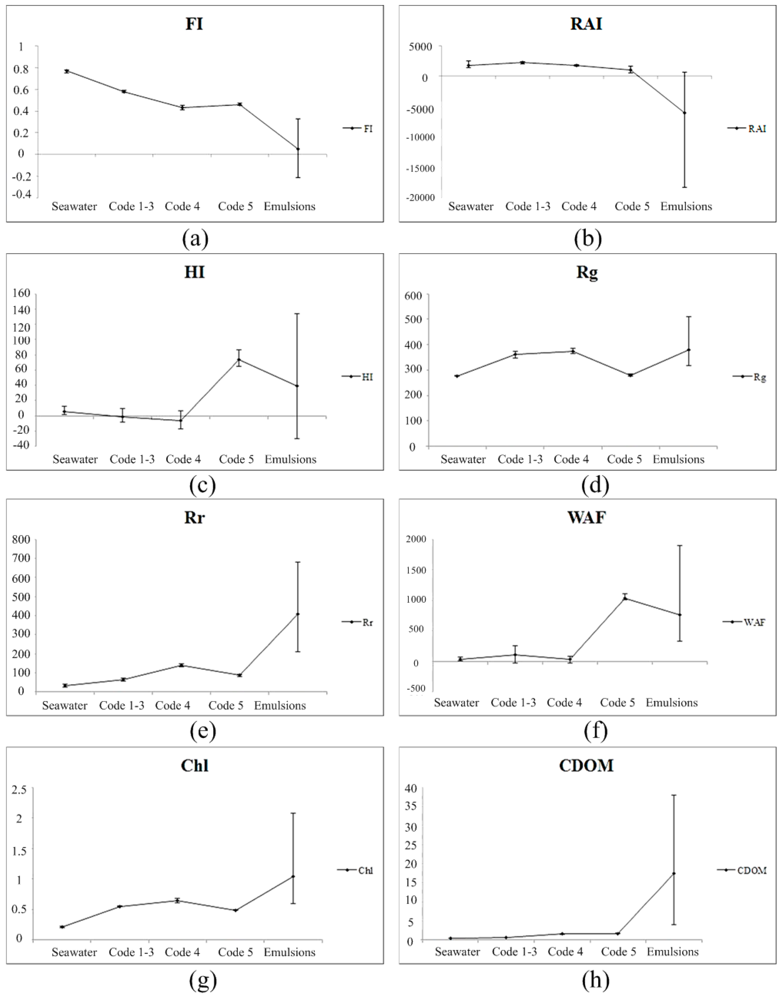
• Differential line graphs based on the training samples.
• The proposed IS measurement.
• Test experiments.

Differential line graphs are summarized from the training results, and the training samples’ spectral indices variation ranges are exhibited in the graphs. These graphs can qualitatively assess a spectral index’s ability to identify oil slicks. The IS measurement also evaluates the identification ability of spectral indices using training results. However, the calculated IS value quantifies the ability. Unlike the aforementioned two methods, testing experiments can evaluate the spectral indices more practically and accurately.

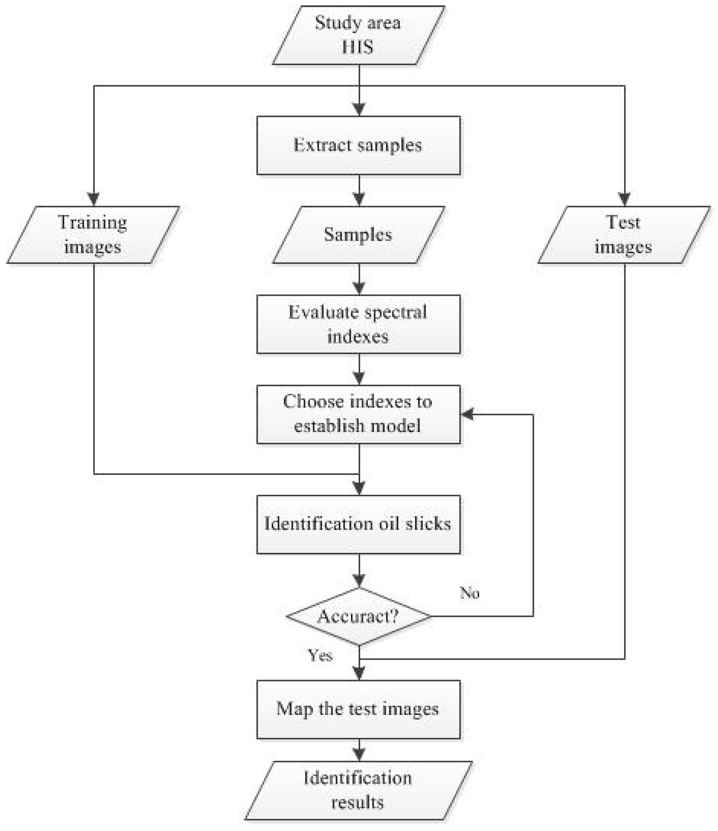
2.6. Experimental Process

To explain the experimental process clearly, a flow chart (Figure 6) is provided in this section. The study area hyperspectral image (HSI) is the atmospheric corrected HIS. The first step of the experiment is extracting training samples, training images, and test areas. Because of the limitation of the oil slick distribution, extracting samples on a large scale would likely introduce error, which may have detrimental effects on the research. Instead, selecting typical samples can ensure the validity of the evaluation. In this research, approximately 10 training samples were selected for each thickness of oil slick or seawater. The training images and test areas must contain different thicknesses of oil slicks and be different from each other. Since the function of the training images is to evaluate spectral indices and select thresholds, their size is smaller than that of the test areas. Numerous hydrocarbon spectral indices have been used to identify oil slicks, and various models have been proposed to assess seawater composition. However, it is not clear which spectral indices are best for detecting thicker oil slicks or sheens. Thus, before the identification model is established, the applicability of the spectral indices of hydrocarbons and seawater must be evaluated qualitatively and quantitatively. After evaluation, the identification model will be established according to the evaluation results to detect oil slicks. The initial thresholds are the median of the training sample distances. To select the proper spectral indices and thresholds, training images are used to optimize the model iteratively. If the model can identify different thicknesses of oil slicks well, the test areas can be used to test the model again to ensure applicability. Finally, the ability of the studied spectral indices can be determined from the evaluation and identification results. At this point, identifying oil slick types will become easier.

3. Results

3.1. Evaluation Results

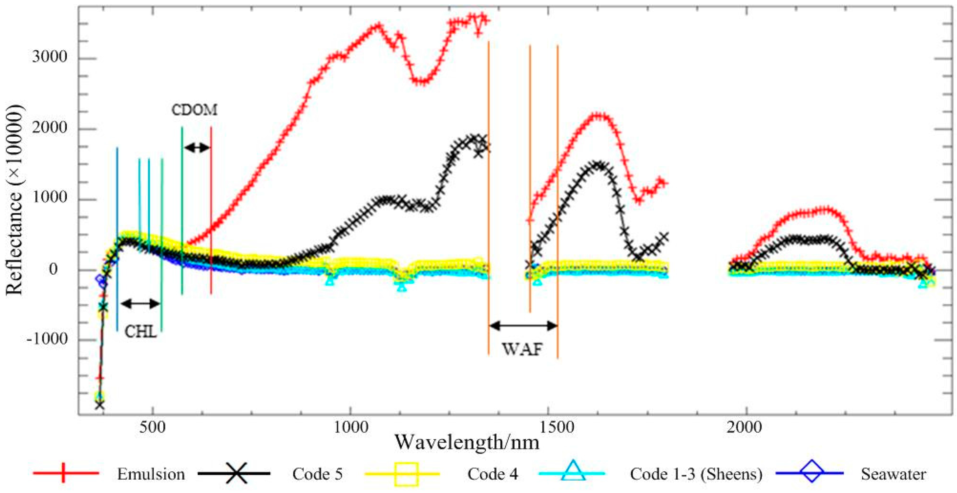
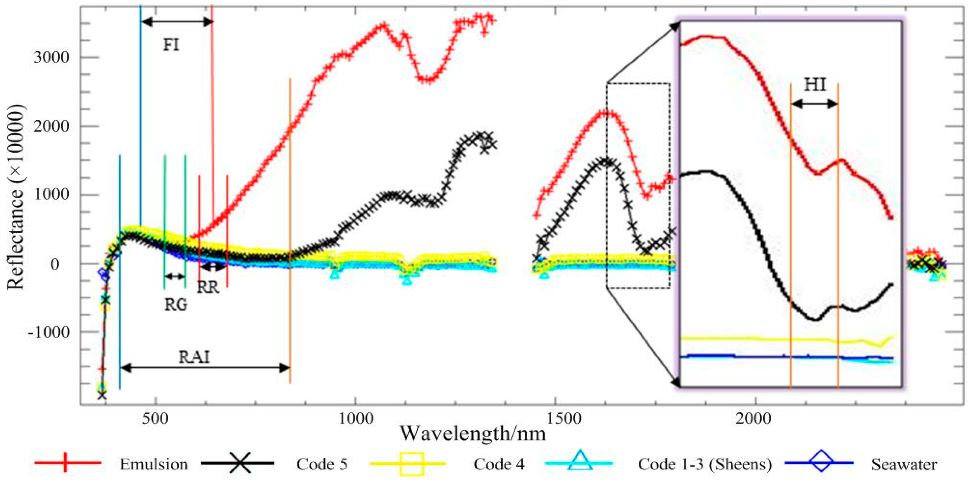
The differential line graph (Figure 7) consists of the fluctuation ranges of the samples’ spectral indices and is used for their qualitative evaluation. Greater sample distance indicates a stronger ability to distinguish the samples. The graphs show that the samples’ fluctuation ranges are limited, except for HI. In addition, emulsions represent a larger range of positive/negative error than true color oil slicks, sheens, and seawater. The limited ranges of the fluctuation indicate that the studied spectral indices are convergent and are thus necessary and important for oil slick identification. The identification ability of HI is unstable because HI is sensitive to the influence of seawater. HI is calculated based on a hydrocarbon substance’s absorption feature, which relies on oil volume. This calculation shows a weak identification ability for sheens, oil slicks of code 4, oil slicks of code 5, and emulsions because they are greatly influenced by seawater. HI is convergent for oil slicks of code 5 oils because they contain a large amount of oil and are seldom influenced by seawater due to the low rate of light transmission. Emulsions had a large positive and negative error because they are mixed substances formed by oil and seawater. The water-to-oil ratio, associated with the degree of emulsification, greatly influences the spectral features. Although the emulsions appeared red or orange, the water-to-oil ratio of the slick is difficult to determine [6], which leads to instability in detecting emulsions.

Based on the differential line graphs, spectral indices can be assessed qualitatively, but it is time-consuming to judge the ability of the spectral indices to identify oil slicks with different thickness using the differential line graphs. To evaluate the spectral indices conveniently and quantitatively, IS values were calculated to assess the ability of the characteristics to differentiate oil slicks. IS values calculated via the training samples are provided in the IS value matrixes (

Table 3. Index separability (IS) values calculated by the training results.

Characteristics	IS Matrixes
FI		Seawater	Sheens	Code 4	Code 5	Emulsions
	Seawater	0	0.3368	1.2121	1.1313	1.697
	Sheens	0.3368	0	0.4848	0.404	0.9697
	Code4	1.2121	0.4848	0	0	0.3232
	Code5	1.1313	0.404	0	0	0.4848
	Emulsions	1.697	0.9697	0.3232	0.4848	0
RAI	Seawater	0	0	0	0	0.1347
	Sheens	0	0	0.0278	0.0589	0.2443
	Code4	0	0.0278	0	0	0.1746
	Code5	0	0.0589	0	0	0
	Emulsions	0.1347	0.2443	0.1746	0	0
HI	Seawater	0	0	0	1.2683	0
	Sheens	0	0	0	0	1.3415
	Code4	0	0	0	0	1.3182
	Code5	1.2683	0	0	0	0
	Emulsions	0	1.3415	1.3182	0	0
RG	Seawater	0	2.3793	2.9655	0	1.3448
	Sheens	2.3793	0	0	2.1379	0
	Code4	2.9655	0	0	2.7241	0
	Code5	0	2.1379	2.7241	0	1.1034
	Emulsions	1.3448	0	0	1.1034	0
RR	Seawater	0	0.1038	0.5557	0.2504	1.0443
	Sheens	0.1038	0	0.3603	0.005	0.8489
	Code4	0.5557	0.3603	0	0.2443	0.4031
	Code5	0.2504	0.005	0.2443	0	0.7328
	Emulsions	1.0443	0.8489	0.4031	0.7328	0
WAF	Seawater	0	0	0	1.9371	0.53
	Sheens	0	0	0	1.5485	0.1413
	Code4	0	0	0	1.9247	0.5175
	Code5	1.9371	1.5485	1.9247	0	0
	Emulsions	0.53	0.1413	0.5175	0	0
CHL	Seawater	0	0.6809	0.8298	0.5532	0.7872
	Sheens	0.6809	0	0.1064	0.1064	0.0638
	Code4	0.8298	0.1064	0	0.2553	0
	Code5	0.5532	0.1064	0.2553	0	0.2128
	Emulsions	0.7872	0.0638	0	0.2128	0
CDOM	Seawater	0	0.0043	0.0991	0.115	0.376
	Sheens	0.0043	0	0.0842	0.1001	0.3611
	Code4	0.0991	0.0842	0	0	0.2503
	Code5	0.115	0.1001	0	0	0.245
	Emulsions	0.376	0.3611	0.2503	0.245	0

).

The rows and columns of the matrix are seawater and oil slicks. The IS values constitute the elements of the IS matrix and are calculated using samples of the corresponding row and column. The matrix is symmetrical, and the diagonal elements of the matrix are all zeros. If the non-diagonal elements were larger than zero, it means that the spectral index could distinguish the row and column. Higher values of the elements indicate a stronger discrimination ability. From the IS matrixes of the spectral indices, it could be observed that:

• The values of $I{S}_{Emulsion,*}^{FI}$, $I{S}_{Emulsion,*}^{RR}$, and $I{S}_{Emulsion,*}^{CDOM}$ are larger than zero, which means that FI, RR (hydrocarbons), and CDOM can be used to distinguish emulsions from seawater and other oil slicks. The “*” means the other categories of the element set {seawater, sheens, oil slicks of code 4, oil slicks of code 5, emulsions}.
• The values of $I{S}_{Seawater,*}^{FI}$, $I{S}_{Seawater,*}^{RR}$, and $I{S}_{Seawater,*}^{CHL}$ are larger than zero, which means that FI, RR, and CHL may be able to distinguish seawater from oil-contaminated areas. Although the values of $I{S}_{Seawater,*}^{CDOM}$ are nonzero, $I{S}_{Seawater,Sheens}^{CDOM}$ is 0.0043 which is too close to zero, so CDOM was not considered during test experiments.
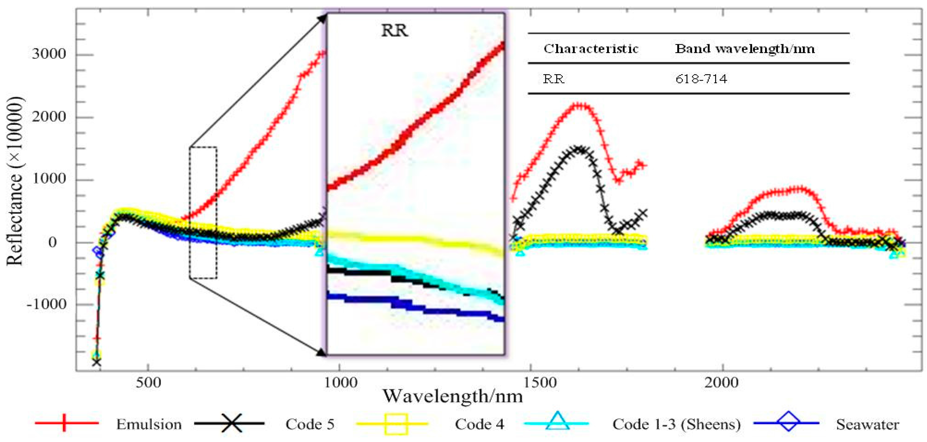
• RR is the only spectral characteristic for which all the non-diagonal elements larger than zero, which means that RR may be able to identify seawater and all thicknesses of oil slicks.
• There is an obvious complementarity of spectral indices of hydrocarbon substance and spectral indices of seawater.

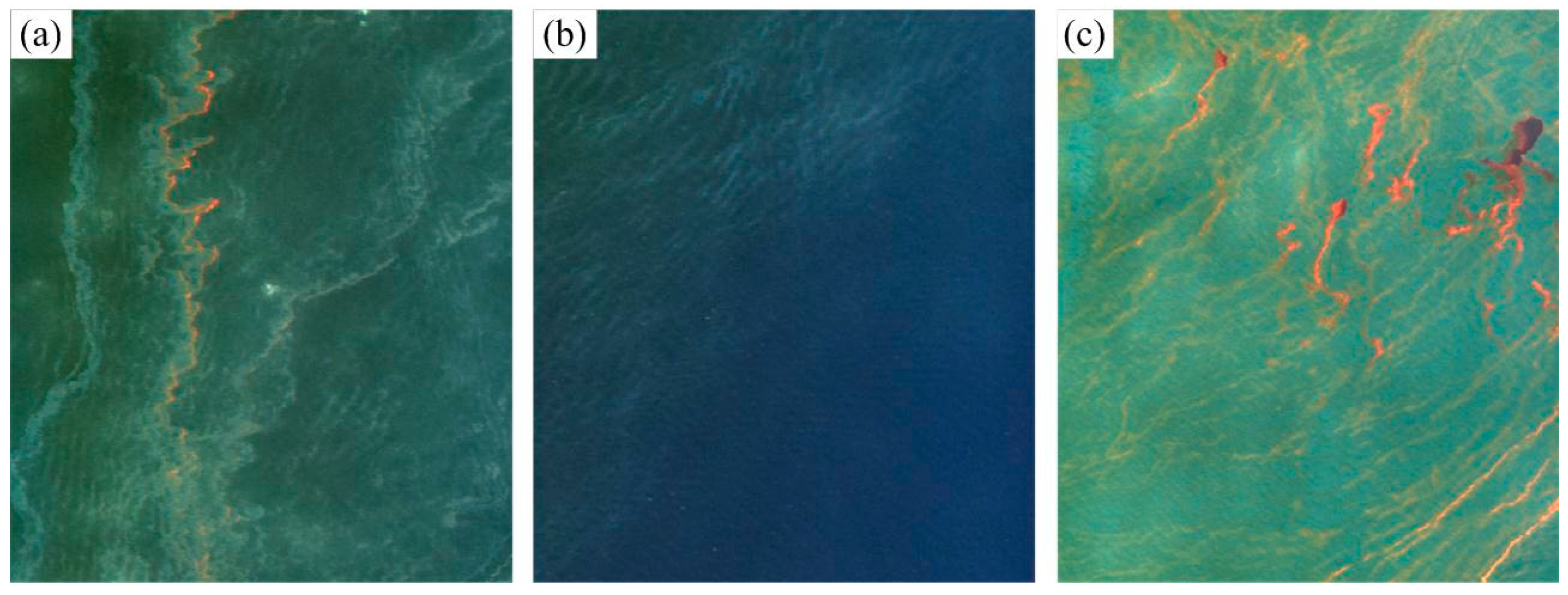
3.2. Identification Results

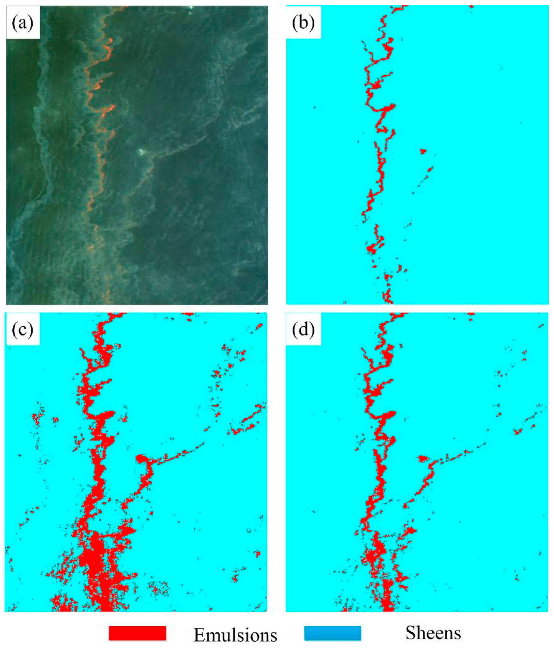
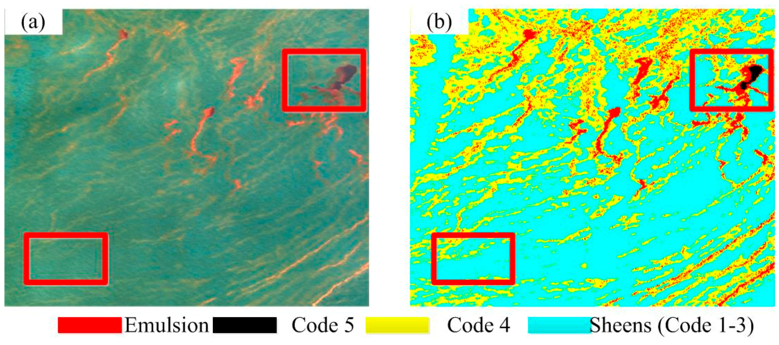
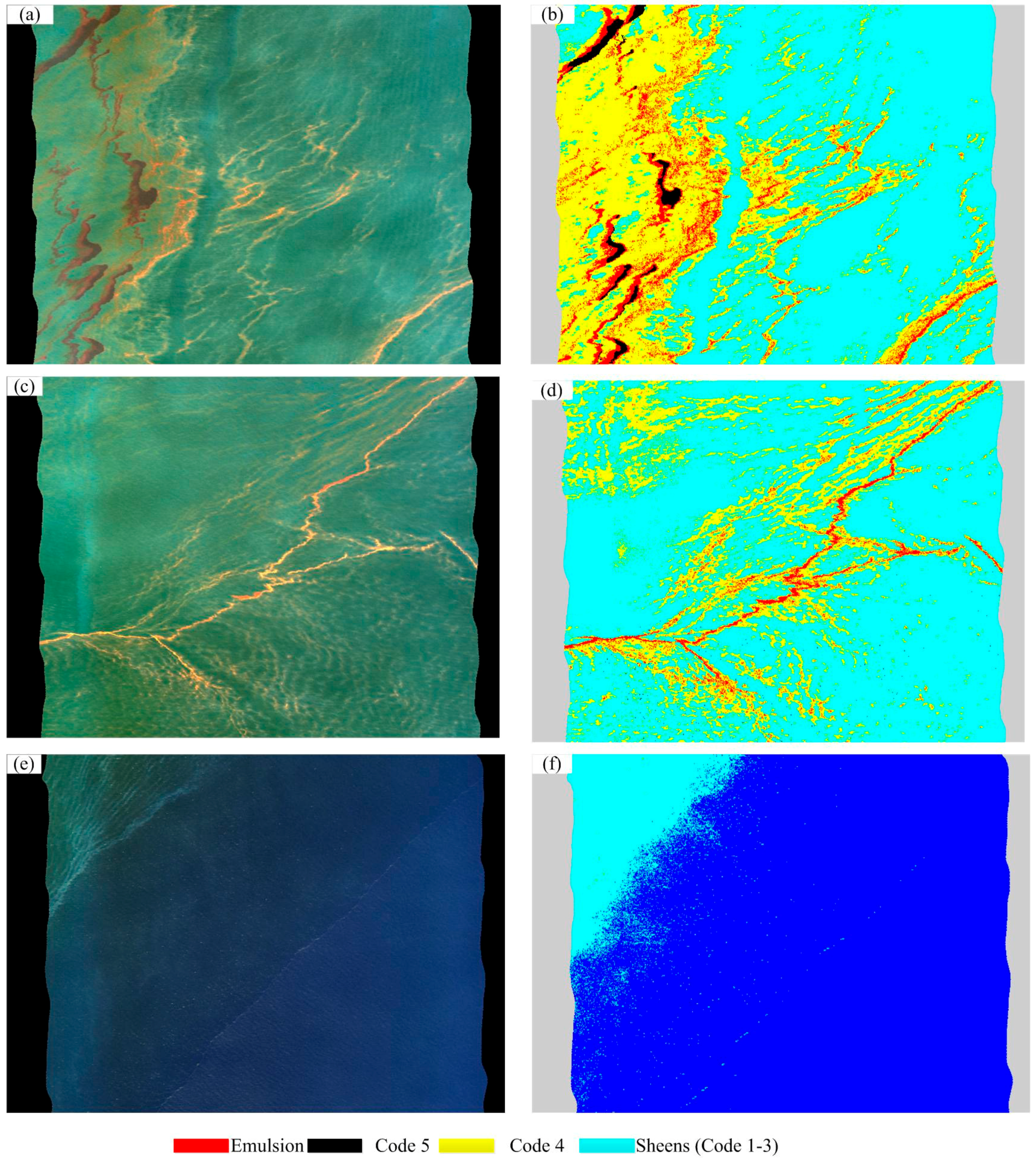
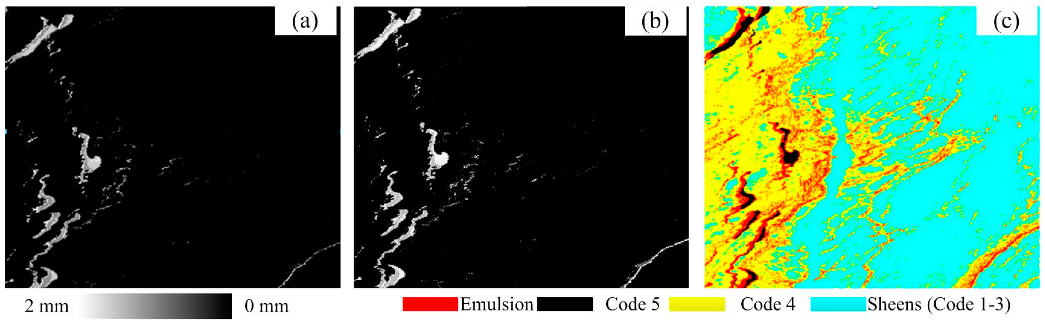
3.2.1. Results of Detecting Emulsions

Test experiments were conducted to verify the aforementioned evaluation results. Since there was a clear band of emulsion surrounded by sheens, training image (a) was used to validate FI, RR, and CDOM’s ability to detect emulsions. Notably, the thresholds selected to identify oil slicks are the central values of the minimum characteristic distance. During identification experiments, several iterations may be conducted to optimize the thresholds. The identification results for detecting emulsions are shown in Figure 8. In the identification results, FI showed the best identification performance. The emulsion band in training image (a) was accurately extracted by FI, and sheens were rarely misidentified. In the results for RR and CDOM, many emulsions were wrongly identified. According to the results of training image (a), FI can better identify emulsions.

FI can detect emulsions because it can detect the spectral characteristics of oil florescence, and thicker oil slicks show stronger florescence than sheens. It is apparent from the spectral curves (Figure 9) that although the bands used by FI exhibit minute differences for distinguishing emulsions from sheens, the trends of spectral curves of sheens and emulsions are entirely different. The normalized ratio method identifies emulsions well. For RR, although emulsions have higher emissivity, which will lead to stronger spectral signals in the longer wavelength bands [16], emulsions exhibit no stable reflectance in red bands due to the unstable water-to-oil ratio. Thus, RR is not effective for detecting emulsions among sheens. CDOM is proposed to evaluate seawater composition. Clean seawater and oil-covered/contaminated seawater should have different CDOM values. CDOM uses green and red bands to establish an exponential model. However, in the results, CDOM indicates that the exponential method weakens the ability to detect emulsions. Numerous sheens were misidentified as emulsions, and thus, CDOM cannot effectively detect emulsions section.

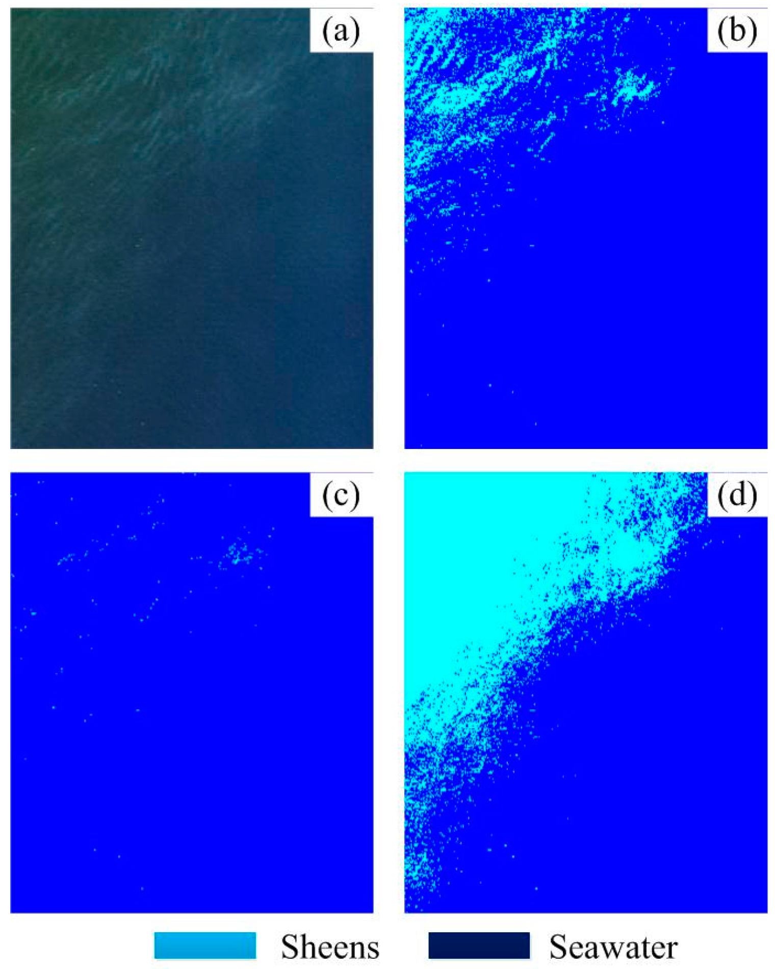
3.2.2. Results of Detecting Sheens

In handling oil spill accidents, it is important to determine the scope of an oil-contaminated area. The core task is accurately distinguishing between sheens (or the least contaminated seawater) and seawater. However, the spectra of sheens are very similar to seawater. Based on the evaluation results, training image (b) was used to validate the ability of FI, RR, and CHL to discriminate seawater and sheens. The test results are shown in Figure 10. CHL identifies sheens from seawater best; compared to FI and RR, there is a rough boundary line of seawater and sheens in the test result of CHL. The FI results are not accurate because the identified sheens are dispersed, whereas the sheens in training image (b) are integrated. RR only poorly identified oil slicks.

FI can be used to discriminate sheens from clean seawater because sheens contain hydrocarbon substances. Sheens can be detected via the spectral characteristics of fluorescence. However, the spectral characteristics of fluorescence for sheens are weak. In Figure 11, the bands of blue and red, representing curves for sheens and seawater, are nearly parallel, meaning that FI can only barely distinguish sheens from seawater. The spectra of sheens and seawater show tiny differences in the red bands. Sheens at the frontier of a spill are extremely thin. They contain less oil and have higher transmittance, thus it is difficult to identify them using visible bands. However, CHL is sensitive to subtle changes in the composition of seawater and can monitor the changes in the spectral curve caused by the covering sheens. Thus, CHL is the best spectral indices for detecting sheens.

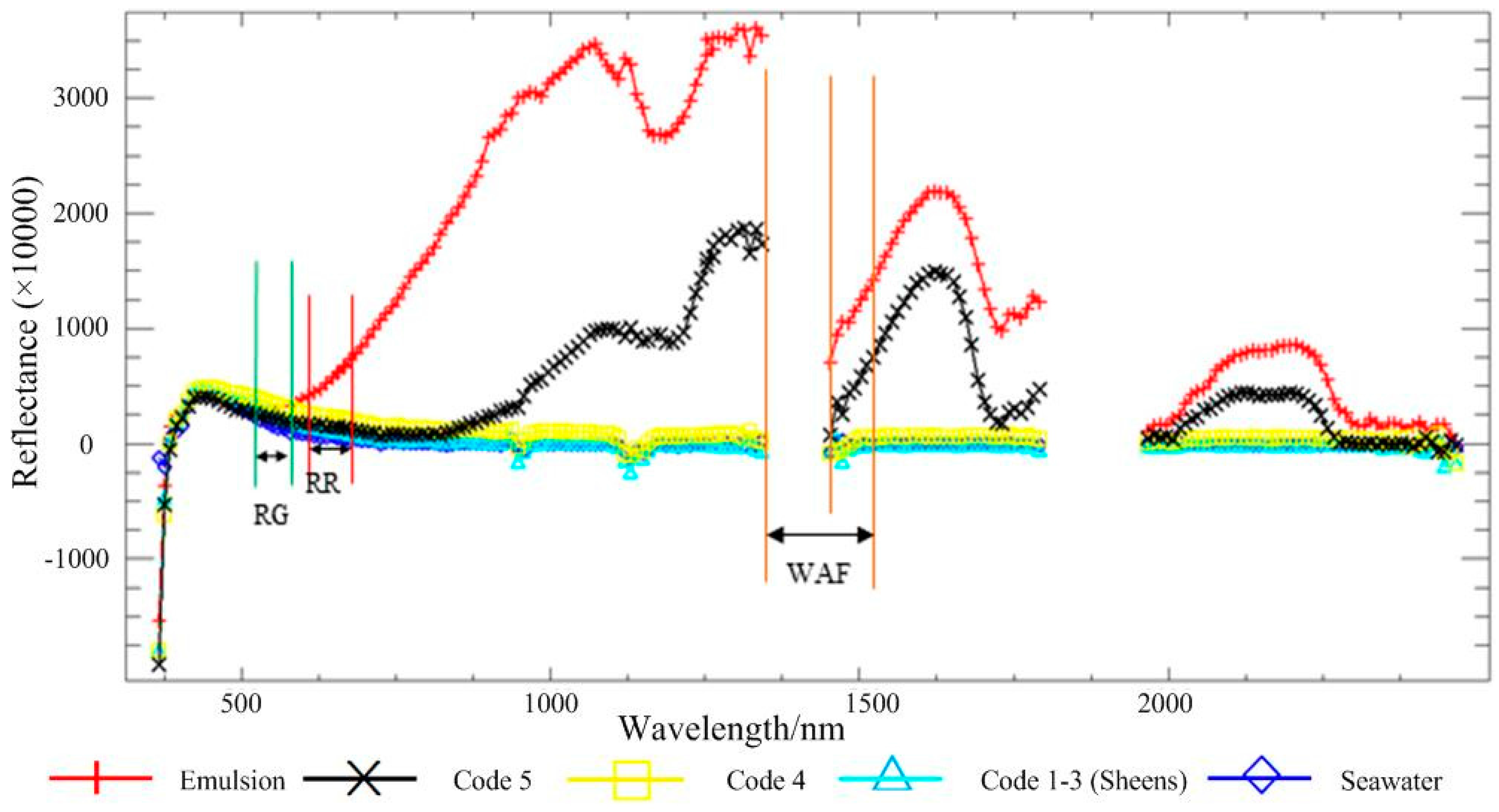
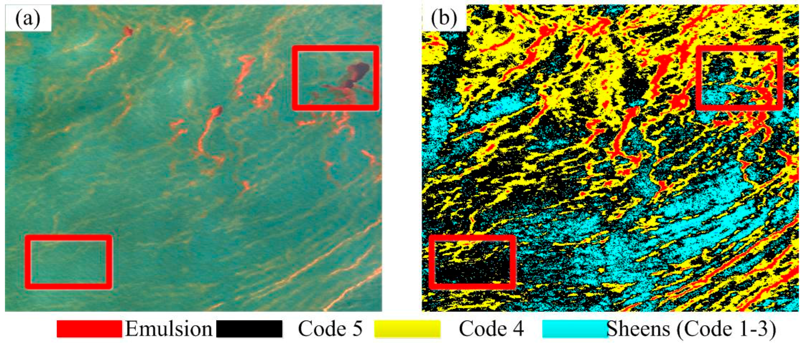
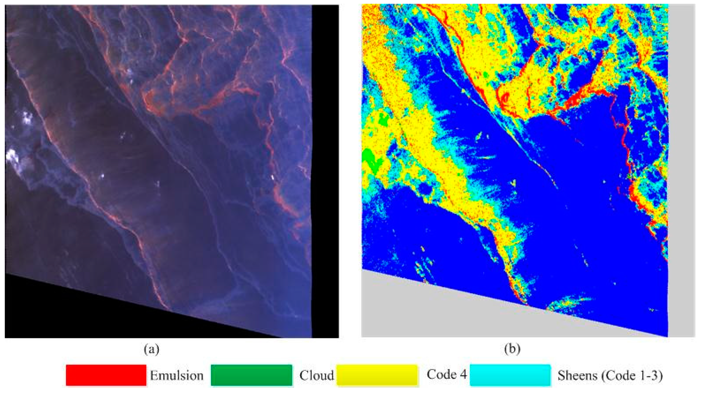
3.2.3. Detection of Oil Slicks by Hydrocarbons (RR)

The IS matrix of RR indicated that RR can identify different thicknesses of oil slicks. Training image (c) was used to validate its performance. This training image contains sheens, true color oil slicks, and emulsions—thus, it is appropriate for verifying the ability of spectral features to identify oil slicks. The identification result is shown in Figure 12; there are several misidentified oil slicks of code 5 and sheens, especially in the red boxes.

The identification results of RR show the opposite conclusion to that of the evaluation result using the IS matrix for the following three reasons:

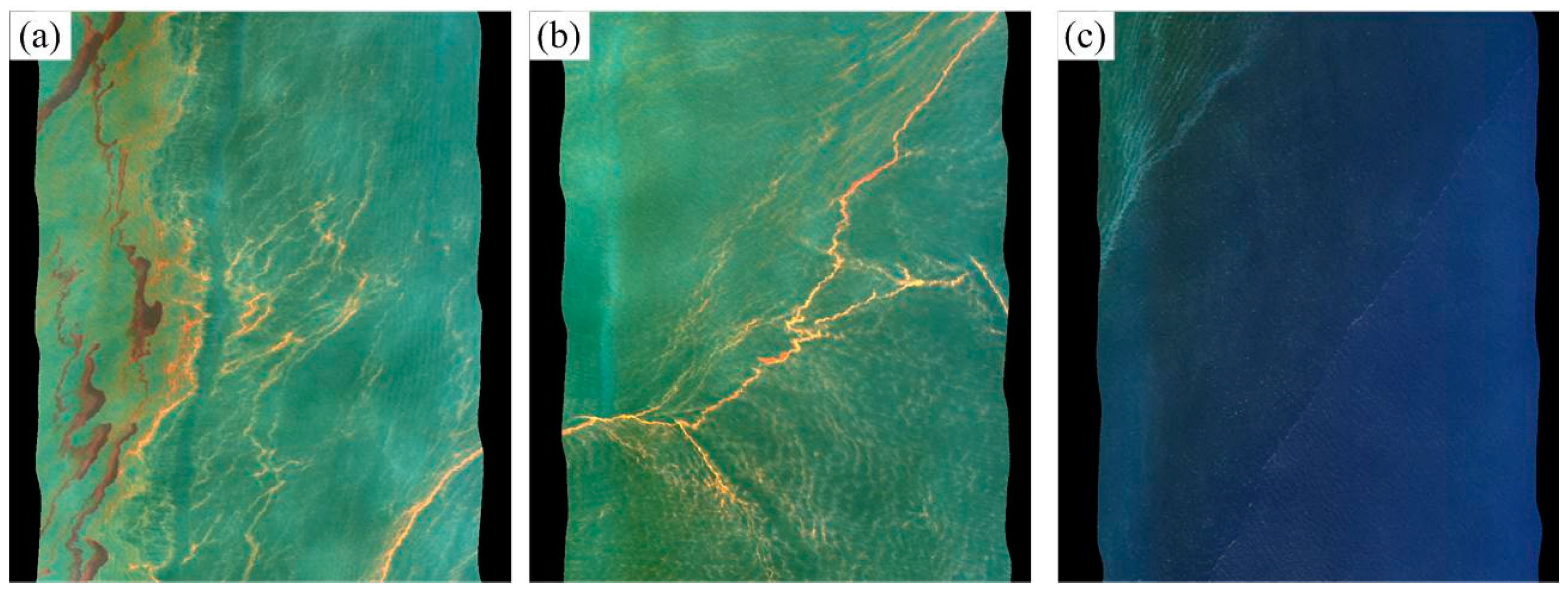
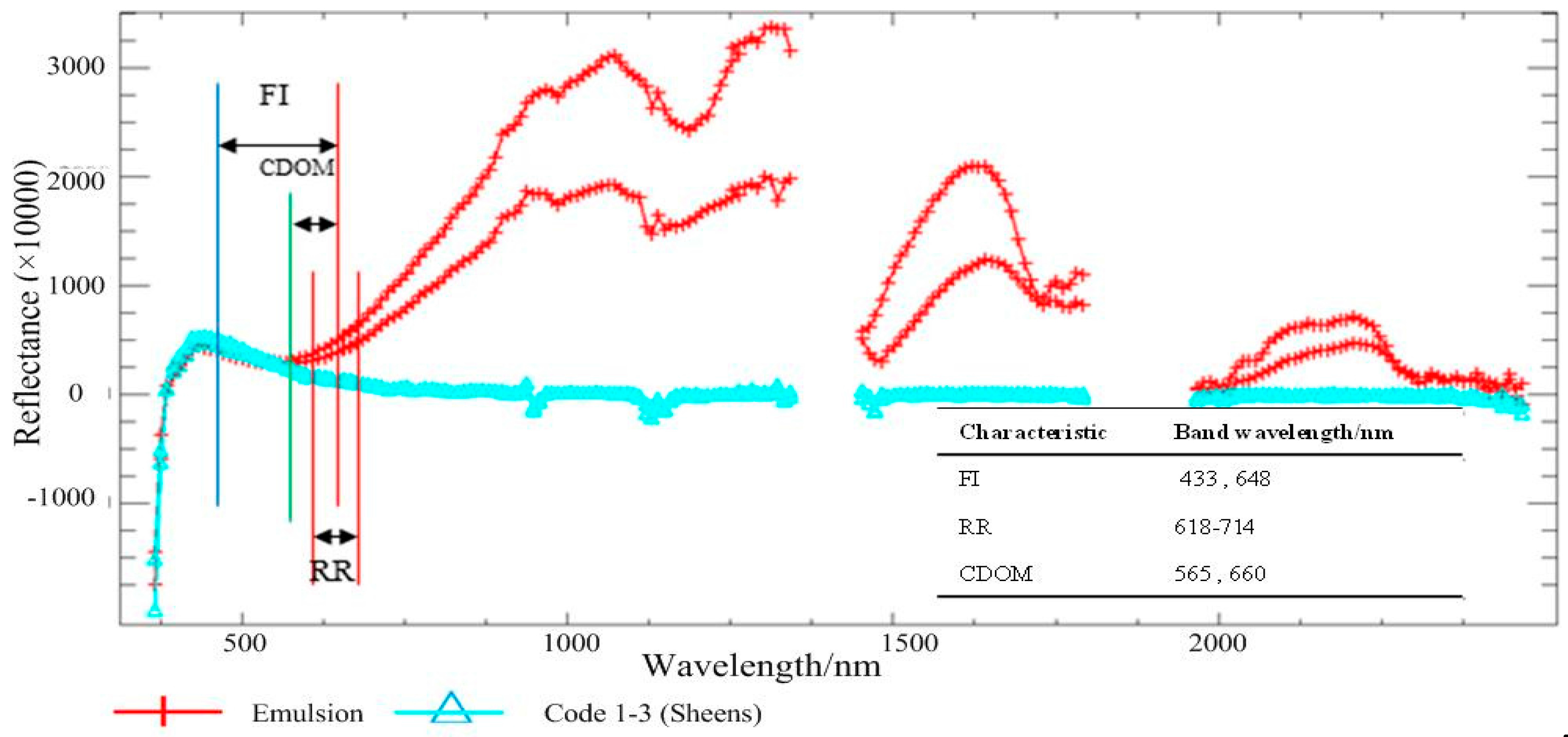
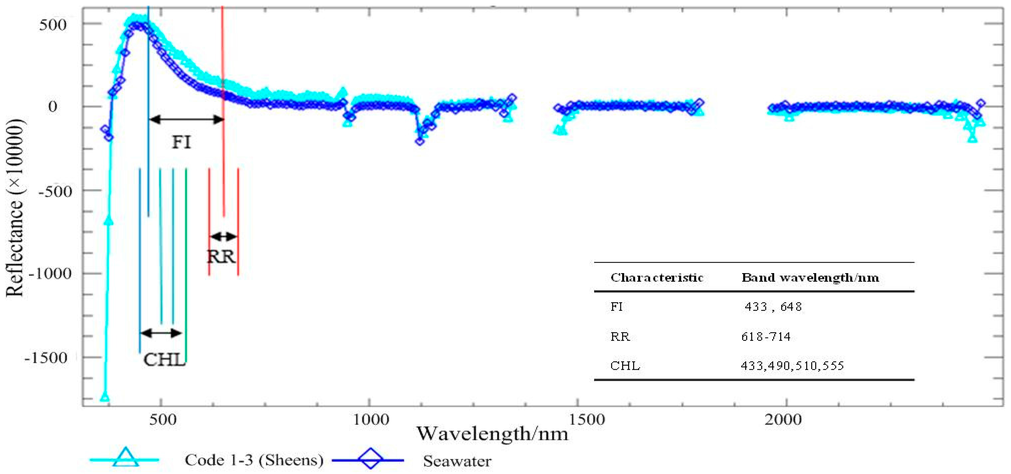
• In the differential line graph of RR (Figure 7), the ranges of sheens and continuous true color oil slicks are small, making it very likely that RR will misidentify sheens and oil slicks of code 5.
• In the spectral curves of seawater and oil slicks in red bands (Figure 13), the curves of sheens and oil slicks of code 5 are nearly coincident, indicating that it is not possible to distinguish sheens and continuous true color oil slicks using RR. In addition, it is difficult for RR to distinguish oil slicks of code 5 from oil slicks of code 4 and sheens according to the spectral analysis.
• In the IS matrix of RR, the IS values of oil slicks of code 5 and sheens are 0.005, which is too close to 0 meaning that RR cannot reliably distinguish between oil slicks of code 5 and sheens. This result is also consistent with the actual recognition results.

Thus, RR identification results were poor, and RR alone cannot accurately identify oil slicks.

3.2.4. Detection of Oil Slicks by Complementary Spectral Indices

As seen in the IS matrixes, the studied spectral indices of hydrocarbons and seawater may have a kind of complementarity. For example, the values of $I{S}_{Emulsion,*}^{RR}$ are 1.0443, 0.8489, 0.4031, and 0.732, and the values of $I{S}_{Emulsions,*}^{WAF}$ are 0.53, 0.1413, 0.5175, and 0. Thus, if RR and WAF are combined to identify emulsions, the characteristic separability will be at least 1.0443, 0.8489, 0.5175, and 0.732, and emulsions can be identified more correctly. By analyzing the IS matrixes, it is apparent that RG and WAF are complementary for identifying emulsions and oil slicks of code 5, and CHL and FI are complementary for identifying sheens and oil slicks of code 4. Thus, a model was established to identify different thicknesses of oil slicks. In the model, CHL is used to distinguish oil-contaminated water from seawater. Training image (c) was used to conduct the experiment. However, some areas were also emulsions misidentified as oil slicks of code 5. Since the IS value of RR to distinguish between oil slicks of code 5 and emulsions was 0.7328, RR was added to detect continuous true color oil slicks. The identification result is shown in Figure 14. This result is substantially better than RR’s identification result.

In Figure 15, emulsions and oil slicks of code 5 show absolute differences in WAF from seawater and thinner oil slicks. However, WAF is not appropriate for distinguishing oil slicks of code 5 and emulsions. However, the spectral curve of emulsions and oil slicks of code 5 show differences in the green to red bands. WAF and RR are complementary for identifying emulsions because WAF can be used to distinguish emulsions from oil slicks of code 4 and sheens and RR can be used to distinguish emulsions from oil slicks of code 5. The strategy of combining complementary spectral indices shows excellent performance in detecting emulsions. In addition, WAF can distinguish oil slicks of code 5 from oil slicks of code 4and sheens, and RG and RR can distinguish oil slicks of code 5 from emulsions. Combining WAF, RG, and RR results in good detectability of the oil slicks of code 5 in the training image (c). There are few sheens misidentified as continuous true color oil slicks compared with the result by RR, which indicates that a model using complementary spectral indices can precisely identify different thicknesses of oil slicks.

4. Discussion

4.1. Applicability of Hydrocarbon Spectral Indices

Hydrocarbon spectral indices involved in this research include FI, RAI, HI, RG, and RR. As indicated in Figure 16, all studied hydrocarbon spectral indices showed an apparent ability to identify emulsions and oil slicks of code 5 from sheens or seawater. Thicker oil slicks contain much more hydrocarbons, and therefore, they possess totally different visual and physical properties from sheens. Thus, emulsions and oil slicks of code 5 show obvious spectral differences in the green, red, and infrared bands. Florescence features and C-H absorption features are shown using these spectra, and the studied spectral indices of hydrocarbons are appropriate for detecting thicker oil slicks.

The results detail the analysis of the hydrocarbon spectral indices. It is apparent from the differential line graphs of the hydrocarbon spectral indices (Figure 7a–d) that although the spectral indices of emulsions show violent volatility, emulsions and oil slicks of code 5 can be distinguished from oil slicks of code 4, sheens, and seawater in general. In addition, IS matrixes of hydrocarbon spectral indices can be used to detect emulsions and oil slicks of code 5, as indicated by values of the $I{S}_{Emulsion,*}^{FI}$, which are 1.6970, 0.9697, 0.3232, and 0.4848; which means that emulsions can be detected by their florescence spectral characteristics. The values of $I{S}_{Emulsions,*}^{RR}$ are 1.0443, 0.8489, 0.4031, and 0.7328, which indicate the possibility of detecting emulsions by spectral reflectance in the red bands. The IS values of RG used to distinguish oil slicks of code 5 from sheens and oil slicks of code 4are 2.1379 and 2.7241, which means that RG has an excellent ability to distinguish oil slicks of code 5 from oil slicks of code 4 and sheens. According to the test experiment results, the hydrocarbon spectral indices of the FI can precisely identify emulsions (Figure 10), and RG can be used to identify oil slicks of code 5 (Figure 14). Meanwhile, the only seawater spectral index considered for its ability to detect emulsions shows a weaker identification result than the FI (Figure 10). The evaluation results are consistent with the aforementioned analysis. It can be concluded that hydrocarbon spectral indices are more suitable for detecting emulsions and oil slicks of code 5.

4.2. Applicability of Seawater Spectral Indices

Seawater spectral indices involved in this research include WAF, CHL, and CDOM. From Figure 17, it can be seen that the calculation of CHL uses the visible bands of the spectra. Seawater and oil slicks have no obvious difference in these bands. The identification ability cannot be judged intuitively, but CDOM appears suitable to detect emulsions, as indicated by the IS matrix. However, in the test results (Figure 8), the ability of CDOM to detect emulsions is weaker than that of the spectral indices of hydrocarbons. It can be observed from Figure 17 that the bands used by WAF exhibit minute differences between seawater, sheens, oil slicks of code 4, and oil slicks of code 5, but they show a strong ability to identify emulsions.

The applicability of WAF for identification is shown in the differential line graph (Figure 7h). This ability may be connected to the high reflectance of thicker oil slicks. Influenced by the sea environment, thicker oil slicks also present water absorption features. Their high reflectance strengthens WAF values. As evidenced by the IS matrix of WAF, the elements of WAF used to distinguish between seawater, sheens, and transitional oil slicks of code 5 are zero, and the elements of WAF to identify emulsions and oil slicks of code 5 are nonzero. The identification model took advantage of this property and precisely recognized oil slicks of code 5 and emulsions (Figure 14). Figure 7h suggests that CHL may possess an excellent ability to distinguish seawater from sheens. CHL is calculated with a complicated regression model, using the blue to red bands to assess the concentration of chlorophyll. It is sensitive to tiny spectral changes in seawater. According to the IS matrix of CHL, the elements of CHL used to distinguish sheens from seawater are 0.6809, 0.8298, 0.5532, and 0.7872, which indicates a strong separability for sheens and seawater. The test result also proves the identification ability of CHL (Figure 10). Compared to the hydrocarbon spectral indices (FI and RR), CHL is more suitable for detecting sheens. In summary, seawater spectral indexes help identify thicker oil slicks but are more useful in the identification of sheens and seawater.

4.3. Complementarity

From the aforementioned discussions, it can be surmised that hydrocarbon spectral indices are more suitable for detecting emulsions and oil slicks of code 5, and seawater spectral indices are more suitable for detecting seawater and sheens. However, it is not realistic to detect different thicknesses of oil slicks using only one spectral index, since the spectra change significantly when the oil slick has different thicknesses or degrees of emulsification. Test experiments prove this point (Figure 12). Notably, the spectral indices of seawater and hydrocarbons have a kind of complementarity, as validated by training image (c) (Figure 14). To further prove the correctness and applicability of this conclusion, three test areas of the original image were used to conduct the experiment. The identification results are shown in Figure 18.

In the identification results of test areas, emulsions, oil slicks of code 5, oil slicks of code 4, sheens, and seawater were well identified. Even sheens at the frontier of the spill were identified correctly (Figure 18e,f). The identification model uses the spectral indices of seawater (WAF) and hydrocarbons (RR) to detect emulsions. The results of test areas (Figure 18a–d) indicate that this method exhibits excellent performance for detecting emulsions. Since emulsions and oil slicks of code 5 are both thicker oil slicks, the model uses WAF, RR, and RG to identify oil slicks of code 5. In the identification result, oil slicks of code 5 are also identified correctly (Figure 18a,b). Finally, oil slicks of code 4 and sheens are identified precisely by FI and CHL.

During the identification experiment, the result of test area (a) (Figure 19c) is compared to the thickness inversion results (Figure 19a,b) produced by USGS 2010. Figure 19a is the conservative evaluation result and Figure 19b is the aggressive evaluation result. The thickness is 0–2 millimeters, linear stretched. From the comparison, it is clear that the method proposed by this research can identify different thicknesses of oil slicks. The result from USGS focuses on only thicker oil slicks. The contrast experiment shows the advantage of this research: correct identification of different thicknesses of oil slicks and even sheens.

These experimental results validate the complementarity of seawater and hydrocarbon spectral indices. The complementarity may be caused by two aspects: the sea environment and oil compositions (mainly hydrocarbons). The spectral curves of oil slicks are determined by oil compositions. However, oil slicks are ineluctably influenced by the sea environment via weathering processes and the light transmittance of the floating oil slicks. For thicker oil slicks that contain plenty of oil and have low light transmittance, hydrocarbons greatly influence the spectral curves. If the oil slicks contain little oil and have high light transmittance, the spectral curves of oil slicks will be more similar to seawater. For specific oil slicks, it is difficult to determine which aspect plays the dominant role in the spectral curves of emulsions. However, evaluation and identification results indicate that combining complementary spectral indices can accurately identify oil slicks of different thickness.

4.4. Accuracy and Applicability

It is important to validate the accuracy of the identification results. Due to the clear visual and shape features of oil slicks of code 4, 5, the accuracy of them can be assessed by visual interpretation. A MODIS image (Figure 20) captured on 17 May 2010 and an ASAR image (Figure 21) captured on May 18 2010 were used to validate the accuracy of the sheens produced by the proposed method. It can be found from Figure 20 and Figure 21 that the identified boundary of sheens is near to the oil slick boundaries detected by MODIS and ASAR image. The tiny inconsistence may be caused by two aspects:

(1)

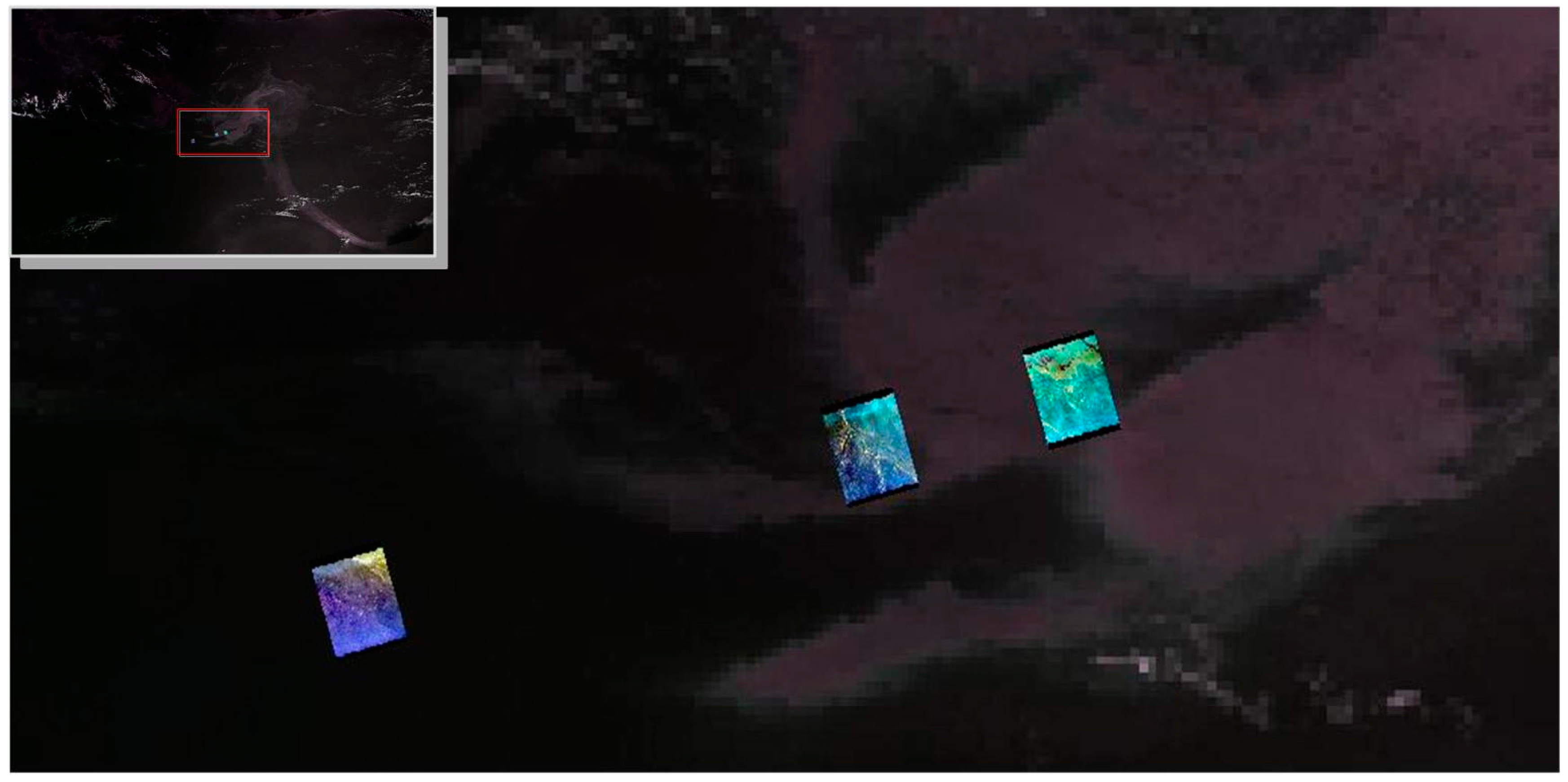
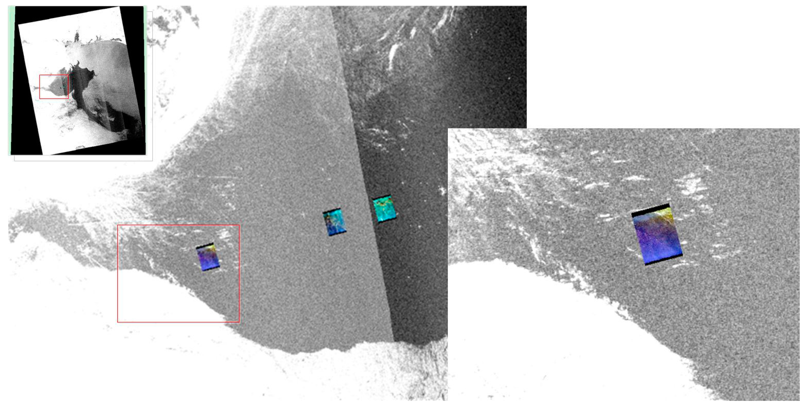
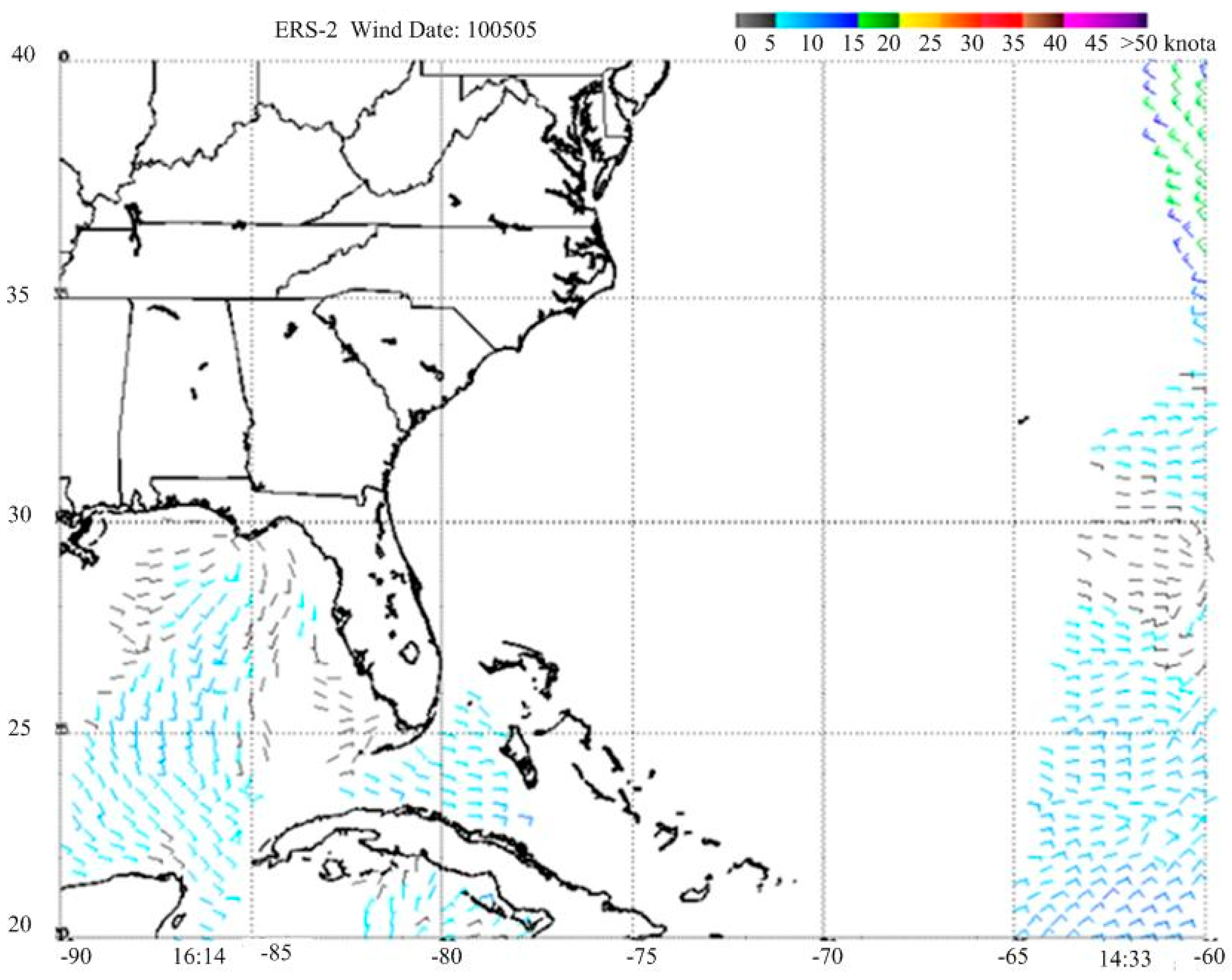
The experimental AVIRIS image was captured at UTC 20:46 17 May 2010, which was later than the MODIS image (UTC 16:40 May 17) and earlier than the ASAR image (UTC 03:48 May 18). The oil slicks in the earlier captured MODIS image do not reach the boundary identified by AVIRIS, but the oil slicks in the later captured ASAR image cover the identified boundary, which means oil slicks drifted during the interval time.

(2)

Sheens at the boundary between oil slicks and seawater cannot be observed from the MODIS and ASAR backscattering images.

Although the research lacked field observations, the AVIRIS, MODIS, and ASAR image can verify the accuracy of the results.

This method can be used to AVIRIS hyperspectral images which are not strongly contaminated by sun glint because it changes the spectral features of oil slicks in a great extent, and spectral indices cannot evaluate the oil slicks and seawater. The image captured on May 17 was used to conduct experiments mainly because it was not influenced by sun glint strongly, and had been proven to be a proper experimental image to validate oil slick identification methods by other researchers [6,8,10]. In order to check the applicability of the conclusions obtained from the research, the proposed method was used to identify oil slicks in another AVIRIS image captured on May 06. The results are shown in Figure 22. It should be noted that the green pixels in Figure 22b are clouds. There are no oil slicks of code 5 in this image, since the oil slicks are influenced by westerly winds (Figure 23) for the experimental image. The oil slicks converge at the west side and spread at the east side. The identified oil slicks with different thicknesses are adjacent and the phenomenon of the thicknesses gradually becoming smaller is well identified by the method.

The accuracy and applicability of the proposed method indicate that the conclusions obtained through the research are accurate and robust.

5. Conclusions

Oil spill accidents are disasters for marine and coastal ecosystems. It is vital to map oil spills when the accidents occur. Hyperspectral images contain abundant spectral information, which is sufficient to identify different thicknesses of oil slicks on the sea surface. However, traditional hyperspectral oil spill mapping methods tend to detect oil slicks using only hydrocarbon spectral indices, and only thicker oil slicks can be identified, as they contain large amounts of oil and have strong hydrocarbon spectral indices. Since the spectral curves of floating oil slicks should be influenced by seawater, based on hyperspectral images, this paper evaluated the spectral indices of both hydrocarbons and seawater. The purpose of the research is to demonstrate the applicability of spectral indices in identifying different thicknesses of oil slicks. In the research, a measurement named IS was proposed to evaluate the ability of the spectral indices to identify oil slicks. Furthermore, the hyperspectral images of the GoM oil spill accident were used to validate the research hypotheses. It can be concluded from the evaluation and identification results that: (1) the spectral indices of hydrocarbons are more suitable for detecting emulsions and continuous true color oil slicks (oil slicks of code 5); (2) the spectral indices of seawater are more suitable for detecting seawater and sheens; and (3) the spectral indices of hydrocarbons and seawater have a kind of complementarity for identifying oil slicks. Combining complementary spectral indices can accurately identify oil slicks with different thicknesses and even identify sheens.

References

1. Alloy, M.; Baxter, D.; Stieglitz, J.; Mager, E.; Hoenig, R.; Benetti, D.; Grosell, M.; Oris, J.; Roberts, A. Ultraviolet radiation enhances the toxicity of Deepwater Horizon oil to mahi-mahi (Coryphaena hippurus) embryos. Environ. Sci. Technol. 2016, 50, 2011–2017. [Google Scholar] [CrossRef] [PubMed]
2. Esbaugh, A.J.; Mager, E.M.; Stieglitz, J.D.; Hoenig, R.; Brown, T.L.; French, B.L.; Linbo, T.L.; Lay, C.; Forth, H.; Scholz, N.L. The effects of weathering and chemical dispersion on Deepwater Horizon crude oil toxicity to mahi-mahi (Coryphaena hippurus) early life stages. Sci. Total Environ. 2016, 543, 644–651. [Google Scholar] [CrossRef] [PubMed]
3. Kokaly, R.F.; Couvillion, B.R.; Holloway, J.A.M.; Roberts, D.A.; Ustin, S.L.; Peterson, S.H.; Khanna, S.; Piazza, S.C. Spectroscopic remote sensing of the distribution and persistence of oil from the Deepwater Horizon spill in Barataria Bay marshes. Remote Sens. Environ. 2013, 129, 210–230. [Google Scholar] [CrossRef]
4. Lammoglia, T.; de Souza Filho, C.R. Chronology and backtracking of oil slick trajectory to source in offshore environments using ultraspectral to multispectral remotely sensed data. Int. J. Appl. Earth Obs. Geoinf. 2015, 39, 113–119. [Google Scholar] [CrossRef]
5. Robla, S.; Sarabia, E.G.; Llata, J.R.; Torre-Ferrero, C.; Pérez Oria, J. An approach for detecting and tracking oil slicks on satellite images. In Proceedings of the OCEANS 2010 MTS/IEEE, Seattle, WA, USA, 20–23 September 2010. [Google Scholar]
6. Clark, R.N.; Swayze, G.A.; Leifer, I.; Livo, K.E.; Kokaly, R.; Hoefen, T.; Lundeen, S.; Eastwood, M.; Green, R.O.; Pearson, N. A Method for Quantitative Mapping of Thick Oil Spills Using Imaging Spectroscopy; US Geological Survey Open-File Report; US Geological Survey: Reston, VA, USA, 2010; Volume 1167, pp. 1–51.
7. Leifer, I.; Lehr, W.J.; Simecek-Beatty, D.; Wozencraft, J.M.; Bradley, E.; Clark, R.N.; Dennison, P.E.; Hu, Y.; Matheson, S.; Jones, C.E. State of the art satellite and airborne marine oil spill remote sensing: Application to the BP Deepwater Horizon oil spill. Remote Sens. Environ. 2012, 124, 185–209. [Google Scholar] [CrossRef]
8. Svejkovsky, J.; Hess, M.; Muskat, J.; Nedwed, T.J.; McCall, J.; Garcia, O. Characterization of surface oil thickness distribution patterns observed during the Deepwater Horizon (MC-252) oil spill with aerial and satellite remote sensing. Mar. Pollut. Bull. 2016, 110, 162–176. [Google Scholar] [CrossRef] [PubMed]
9. Pisano, A.; Bignami, F.; Santoleri, R. Oil spill detection in glint-contaminated near-infrared MODIS imagery. Remote Sens. 2015, 7, 1112–1134. [Google Scholar] [CrossRef]
10. Alam, M.S.; Sidike, P. Trends in oil spill detection via hyperspectral imaging. In Proceedings of the 7th Electrical & Computer Engineering (ICECE), Dhaka, Bangladesh, 20–22 December 2012. [Google Scholar]
11. Li, Q.; Lu, L.; Zhang, B.; Tong, Q. Oil Slope Index: An algorithm for crude oil spill detection with imaging spectroscopy. In Proceedings of the 2012 Second International Workshop on Earth Observation and Remote Sensing Applications, Shanghai, China, 8–11 June 2012. [Google Scholar]
12. Liu, D.; Zhang, J.; Wang, X. Reference spectral signature selection using density-based cluster for automatic oil spill detection in hyperspectral images. Opt. Express 2016, 24, 7411–7425. [Google Scholar] [CrossRef] [PubMed]
13. Kaiser, M.F.; Aziz, A.M.; Ghieth, B.M. Use of remote sensing techniques and aeromagnetic data to study episodic oil seep discharges along the Gulf of Suez in Egypt. Mar. Pollut. Bull. 2013, 72, 80–86. [Google Scholar] [CrossRef] [PubMed]
14. Lu, Y.; Zhan, W.; Hu, C. Detecting and quantifying oil slick thickness by thermal remote sensing: A ground-based experiment. Remote Sens. Environ. 2016, 181, 207–217. [Google Scholar] [CrossRef]
15. Fingas, M.F.; Brown, C.E. Review of oil spill remote sensing. Spill Sci. Technol. Bull. 1997, 4, 199–208. [Google Scholar] [CrossRef]
16. Fingas, M.; Brown, C. Review of oil spill remote sensing. Mar. Pollut. Bull. 2014, 83, 9–23. [Google Scholar] [CrossRef] [PubMed]
17. Otremba, Z. The impact on the reflectance in VIS of a type of crude oil film floating on the water surface. Opt. Express 2000, 7, 129–134. [Google Scholar] [CrossRef] [PubMed]
18. Mityagina, M.; Lavrova, O. Satellite Survey of Inner Seas: Oil Pollution in the Black and Caspian Seas. Remote Sens. 2016, 8, 875. [Google Scholar] [CrossRef]
19. National Aeronautics and Space Administration (NASA). Available online: http://aviris.jpl.nasa.gov/alt_locator (accessed on 5 September 2016).
20. Carpenter, A. The Bonn agreement aerial surveillance programme: Trends in North Sea oil pollution 1986–2004. Mar. Pollut. Bull. 2007, 54, 149–163. [Google Scholar] [CrossRef] [PubMed]
21. Kumar, A.; Suresh, G. Weathering of Oil Spill: Modeling and Analysis. Aquat. Procedia 2015, 4, 435–442. [Google Scholar]
22. Stevens, C.C.; Thibodeaux, L.J.; Overton, E.B.; Valsaraj, K.T.; Nandakumar, K.; Rao, A.; Walker, N.D. Sea surface oil slick light component vaporization and heavy residue sinking: Binary mixture theory and experimental proof of concept. Environ. Eng. Sci. 2015, 32, 694–702. [Google Scholar] [CrossRef]
23. Sun, S.; Hu, C.; Feng, L.; Swayze, G.A.; Holmes, J.; Graettinger, G.; MacDonald, I.; Garcia, O.; Leifer, I. Oil slick morphology derived from AVIRIS measurements of the Deepwater Horizon oil spill: Implications for spatial resolution requirements of remote sensors. Mar. Pollut. Bull. 2016, 103, 276–285. [Google Scholar] [CrossRef] [PubMed]
24. Cong, L.; Nutter, B.; Liang, D. Estimation of oil thickness and aging from hyperspectral signature. In Proceedings of the Image Analysis and Interpretation (SSIAI), Santa Fe, NM, USA, 22–24 April 2012. [Google Scholar]
25. Loos, E.; Brown, L.; Borstad, G.; Mudge, T.; Alvare, M. Characterization of oil slicks at sea using remote sensing techniques. In Proceedings of the OCEANS, Yeosu, Korea, 14–19 October 2012. [Google Scholar]
26. Kühn, F.; Oppermann, K.; Hörig, B. Hydrocarbon Index—An algorithm for hyperspectral detection of hydrocarbons. Int. J. Remote Sens. 2004, 25, 2467–2473. [Google Scholar] [CrossRef]
27. Sun, P. Study of prediction models for oil thickness based on spectral curve. Spectrosc. Spectr. Anal. 2013, 33, 1881–1885. [Google Scholar]
28. Lu, W.Z.; Yuan, H.F.; Xu, G.T. Modern Near Infrared Spectroscopy Analytical Technology; China Petrochemical Press: Beijing, China, 2007. [Google Scholar]
29. Hu, C.; Lee, Z.; Franz, B. Chlorophyll aalgorithms for oligotrophic oceans: A novel approach based on three—Band reflectance difference. J. Geophys. Res. Ocean. 2012, 117. [Google Scholar] [CrossRef]
30. Kutser, T.; Pierson, D.C.; Kallio, K.Y.; Reinarta, A.; Sobeka, S. Mapping lake CDOM by satellite remote sensing. Remote Sens. Environ. 2005, 94, 535–540. [Google Scholar] [CrossRef]
31. Lu, Y.C.; Tian, Q.J.; Qi, X.P.; Wang, J.J.; Wang, X.C. Spectral response analysis of offshore thin oil slicks. Spectrosc. Spectr. Anal. 2009, 29, 986–989. [Google Scholar]
Figure 1. Picture (a) is the experimental data image, false-color composite with bands R: 678 nm, G: 540 nm, and B: 443 nm. Picture (b) is study area scope was obtained via ENVI and Google Earth software.
Remotesensing 10 00421 g001
Figure 2. Three training images used to evaluate the ability of spectral indices to identify diverse thicknesses of oil slicks. Pictures (ac) are false-color composited training images (ac).
Remotesensing 10 00421 g002
Figure 3. Three test areas extracted from the original hyperspectral image to validate the conclusion. Training areas are distinct from these test areas. Pictures (ac) are false-color composited test images (ac).
Remotesensing 10 00421 g003
Figure 4. Oil slick thickness descriptions.
Remotesensing 10 00421 g004
Figure 5. Images of different thicknesses of oil slicks and their spectral curves.
Remotesensing 10 00421 g005
Figure 6. Flow chart of the experimental process (HSI = hyperspectral image).
Remotesensing 10 00421 g006
Figure 7. Differential line graphs of spectral indices of hydrocarbons and seawater are summed from the training results. Pictures (ah) are differential line graphs of FI, RAI, HI, Rg, Rr, WAF, Chl, and CDOM, respectively.
Remotesensing 10 00421 g007
Figure 8. Images (bd) are identification results for emulsions and sheens; red pixels represent identified emulsions, and cyan pixels represent sheens. Photo (a) is the original training image, and (bd) are the identification results of FI (fluorescence index), RR (hydrocarbons), and CDOM (Colored Dissolved Organic Matter), respectively.
Remotesensing 10 00421 g008
Figure 9. Spectral curve analysis identifying emulsions (red) and sheens (cyan) using FI, RR, and CDOM.
Remotesensing 10 00421 g009
Figure 10. Images (bd) are identification results for seawater and sheens; cyan pixels represent identified sheens and blue pixels represent seawater. Photo (a) is the original training image, and (bd) are identification results for FI, RR, and CHL, respectively.
Remotesensing 10 00421 g010
Figure 11. Spectral curve analysis for identifying sheens (cyan) and seawater (blue) by FI, RR, and CHL.
Remotesensing 10 00421 g011
Figure 12. Photo (a) is the original training image, and image; (b) is the identification result: red pixels represent identified emulsions, black pixels are oil slicks of code 5, yellow pixels are oil slicks of code 4, and cyan pixels are sheens.
Remotesensing 10 00421 g012
Figure 13. Spectral curve analysis identifying different thickness of oil slicks by RR. Red, black, yellow, cyan, and blue lines represent emulsions, oil slicks of code 5, oil slicks of code 4, oil slicks of code 1–3, and seawater, respectively.
Remotesensing 10 00421 g013
Figure 14. Photo (a) is the original training image, and picture (b) is the identification result. In the results, red pixels represent identified emulsions, black pixels are oil slicks of code 5, yellow pixels are oil slicks of code 4, and cyan pixels are sheens.
Remotesensing 10 00421 g014
Figure 15. Bands of spectral indices used by RR, RG, and WAF. Red, black, yellow, cyan, and blue lines represent emulsions, oil slicks of code 5, oil slicks of code 4, oil slicks of code 1–3, and seawater, respectively.
Remotesensing 10 00421 g015
Figure 16. Bands used for spectral indices of hydrocarbons. Red, black, yellow, cyan, and blue lines represent emulsions, oil slicks of code 5, oil slicks of code 4, oil slicks of code 1–3, and seawater, respectively.
Remotesensing 10 00421 g016
Figure 17. Bands used for seawater spectral indices. Red, black, yellow, cyan, and blue lines represent emulsions, oil slicks of code 5, oil slicks of code 4, oil slicks of code 1–3, and seawater, respectively.
Remotesensing 10 00421 g017
Figure 18. Three test areas used to validate the complementarity of spectral indices of hydrocarbons and seawater. Pictures (a,c,e) are the false-color composited test images (a,b,c), respectively. Pictures (b,d,f) are the identification results of test images (a,b,c), respectively.
Remotesensing 10 00421 g018
Figure 19. Photo (a,b): thickness results from USGS 2010. Picture (c): thickness results produced in this work.
Remotesensing 10 00421 g019
Figure 20. The identification results of this research and MODIS image captured at UTC 16:40 17 May 2010.
Remotesensing 10 00421 g020
Figure 21. The identified results of this research and ASAR backscatter image captured at UTC 03:48 18 May 2010.
Remotesensing 10 00421 g021
Figure 22. Identification results of another Airborne Visible Infrared Imaging Spectrometer (AVIRIS) image captured on 6 May 2010. Picture (a) is the false-color AVIRIS composited image and picture (b) is the identification result of it.
Remotesensing 10 00421 g022
Figure 23. Wind image of Gulf of Mexico on 6 May 2010.
Remotesensing 10 00421 g023