Article

An Object-Based Image Analysis Method for Enhancing Classification of Land Covers Using Fully Convolutional Networks and Multi-View Images of Small Unmanned Aerial System

1
School of Forest Resources and Conservation, University of Florida, Gainesville, FL 32611, USA
2
Gulf Coast Research Center, University of Florida, Plant City, FL 33563, USA
*
Author to whom correspondence should be addressed.
Remote Sens. 2018, 10(3), 457; https://doi.org/10.3390/rs10030457
Submission received: 15 February 2018 / Revised: 5 March 2018 / Accepted: 10 March 2018 / Published: 14 March 2018
(This article belongs to the Section Remote Sensing Image Processing)

Abstract

:
Fully Convolutional Networks (FCN) has shown better performance than other classifiers like Random Forest (RF), Support Vector Machine (SVM) and patch-based Deep Convolutional Neural Network (DCNN), for object-based classification using orthoimage only in previous studies; however, for further improving deep learning algorithm performance, multi-view data should be considered for training data enrichment, which has not been investigated for FCN. The present study developed a novel OBIA classification using FCN and multi-view data extracted from small Unmanned Aerial System (UAS) for mapping landcovers. Specifically, this study proposed three methods to automatically generate multi-view training samples from orthoimage training datasets to conduct multi-view object-based classification using FCN, and compared their performances with each other and also with RF, SVM, and DCNN classifiers. The first method does not consider the object surrounding information, while the other two utilized object context information. We demonstrated that all the three versions of FCN multi-view object-based classification outperformed their counterparts utilizing orthoimage data only. Furthermore, the results also showed that when multi-view training samples were prepared with consideration of object surroundings, FCN trained with these samples gave much better accuracy than FCN classification trained without context information. Similar accuracies were achieved from the two methods utilizing object surrounding information, although sample preparation was conducted using two different ways. When comparing FCN with RF, SVM, DCNN implies that FCN generally produced better accuracy than the other classifiers, regardless of using orthoimage or multi-view data.

Graphical Abstract

1. Introduction

Small Unmanned Aircraft System (UAS), has become a popular remote sensing platform for providing very high-resolution images targeting small or medium size sites in the past decade, due to its advantages of safety, flexibility, and low-cost over other airborne or space-borne platforms. The continuous technical advancements that have improved its payload and durance over the years significantly contributed to its increased utilization, a trend not expected to slow down soon [1,2]. Object-based Image Analysis (OBIA) has been routinely employed to process UAS images for landcover mapping, with its capability of generating more appealing maps and comparable (if not higher) classification accuracy when compared with pixel-based methods [3,4,5,6,7,8]. Analyzing the UAS images using traditional OBIA normally starts with bundle adjustment procedure to produce orthoimage from all the UAS images. Then, image segmentation algorithm is conducted to segment the orthoimage to groups of homogeneous pixels to form numerous meaningful objects. Spectral, geometrical, textural, and contextual features are extracted from these objects and used as input to different classifiers, such as Random Forest (RF) [9] and Support Vector Machine (SVM) [10], to label the objects. Feature extraction and selection that have to be conducted during traditional OBIA procedures are challenging tasks and can limit classification performance.
Recently, the rise of deep learning techniques provided an alternative to traditional land cover classifiers. Deep learning brought about around 2006 [11], became well known in the computer vision community around 2012, since one supervised version of deep learning networks Deep Convolutional Neural Networks (DCNN) made a breakthrough for scene classification tasks [12,13], and has reached out to many industrial applications and other academic areas in recent years as it continues to advance technologies in areas, like speech recognition [14], medical diagnosis [15], autonomous driving [16], or even the gaming world [17,18]. When compared with other traditional classifiers, deep learning does not require feature engineering, which attracted many researchers from the remote sensing community to test its usability for landcover mapping [19,20,21,22,23]. Two latest review papers [20,24] on OBIA both also emphasize the need for testing deep learning techniques under the OBIA framework.
Deep learning networks normally have a huge number of parameters to be adjusted during the training procedure and may require massive training samples to trigger its power, as shown in one of the latest studies [25], but collecting training samples is expensive for remote sensing applications. To overcome the scarce training samples limitation, several strategies have been proposed, such as augmenting the limited labeled samples with various transformation operations, such as rotation, translation and scaling [26,27], unsupervised pre-training [11,28], transfer learning [29,30], etc. Multi-view data collected by small UAS naturally expands the training dataset, thanks to the bidirectional reflectance effect resulting from the changes in view and illumination angles along the image acquisition mission. Multi-view data has been proved useful for vegetation in several publications [31,32,33,34]. Most of the applications relied on bidirectional reflectance distribution function (BRDF) modeling to extract BRDF 3–5 parameters as part of landcover features to utilize the multi-view information for landcover mapping. However, this type of method is inefficient and inapplicable for the deep learning classifiers to utilize the multi-view information, since DCNN or FCN extract features automatically within as part of the classifier training process.
We recognize two types of convolutional neural networks for deep learning techniques that are applicable for land cover mapping tasks: The first one assigns single class label to the whole input image patch, while the other one assigns class labels to each individual pixel within input image patch. We refer to the first type as Deep Convolutional Neural Network (DCNN) and the second type as Fully Convolutional Network (FCN) [35]. FCN has been used to deal with various computer vision related problems successfully in recent years since its introduction, such as liver cancer diagnosis via analysis of cancerous tissue pathological image [36], diagnosis of smaller bowel disease through automatically marking cross-sectional diameters on small bowel images [37], osteosarcoma tumor segmentation on computed tomography (CT) images [38], traffic sign detection [39], etc. Applications using FCN in remote sensing domain can also be found, even though their number is still small. Most of these studies were conducted using the ISPRS Vaihingen dataset achieves [40]. This data set contains 8 cm resolution Near Infrared (NIR), Red (R), and Green (G) bands orthoimage, point cloud (4 points/m2), and 9 cm resolution Digital Surface Model (DSM) of an urban area. This dataset was collected for urban object detection and has been used by several studies comparing FCN with other classifiers such as DCNN and random forest [41,42,43].
A recent study by Liu et al. [25] conducted a comprehensive comparison among FCN, DCNN, RF, and SVM performances under the OBIA framework, when considering the impact of training sample size. The study concluded that DCNN might produce inferior performance as compared to conventional classifiers when the training sample size is small, but it tends to show substantially higher accuracy when the training sample size increases. Their results also indicated that FCN is more efficient in exploiting the information in the training samples than the other classifiers achieving higher accuracy in most cases regardless of sample size.
This study extends the study of Liu et al. [25] by developing novel methods via photogrammetric techniques to enable the FCN to utilize the multi-view data extracted from UAS images to investigate whether the enriched training samples resulting from multi-view data extraction can further improve the FCN performance and also compare FCN with other classifiers under this multi-view OBIA framework regarding the multi-view data impacts on their performances, in order to find the best practice of applying FCN for land cover mapping.

2. Study Area and Data Preprocessing
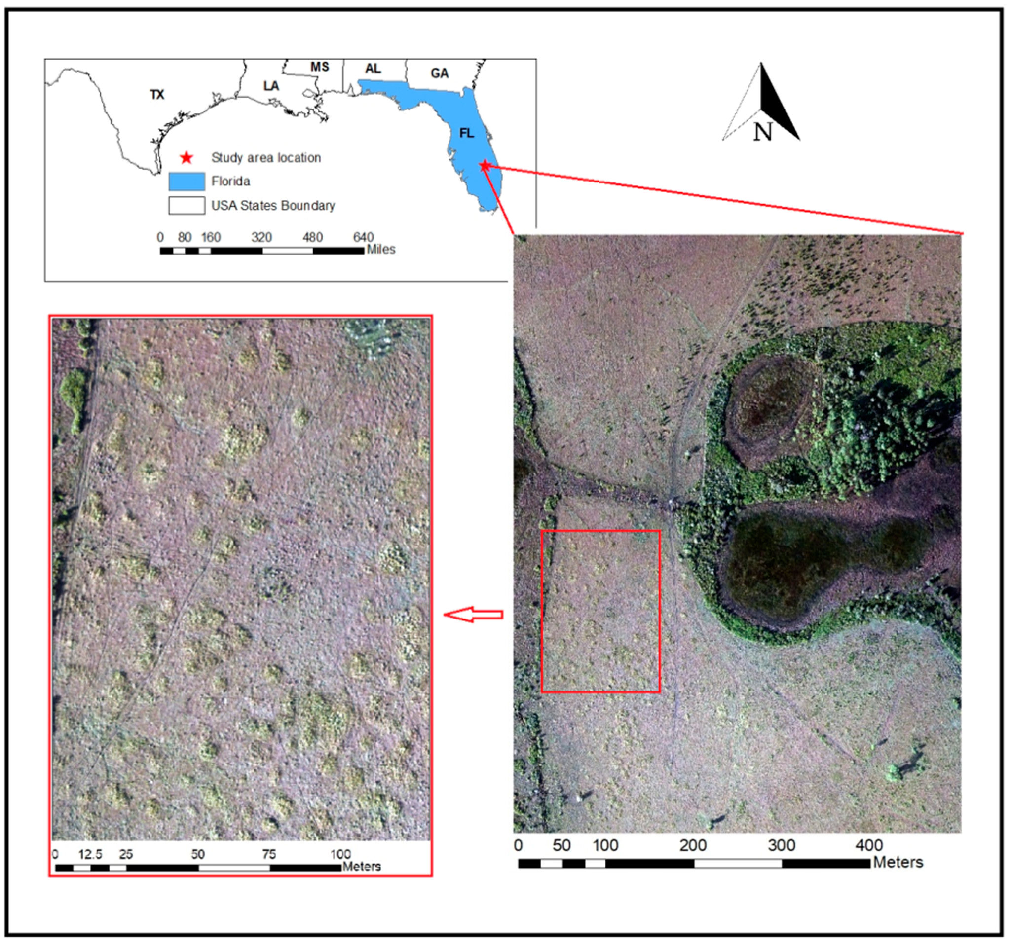
2.1. Study Area

The proposed classification methods were tested on a 677 m × 518 m area, which is part of a 31,000-acre ranch, located in Southern Florida, between Lake Okeechobee and the city of Arcadia. The ranch is comprised of diverse tropical forage grass pastures, palmetto wet and dry prairies, pine flatwoods, and large interconnecting marsh of native grass wetlands [44]. The land also hosts cabbage palm and live oak hammocks scattering along the lengths of copious creeks, gullies, and wetlands. The study area is infested by Cogon grass (Imperata Cylindrical), as shown in the lower left corner of Figure 1, scattered across the pasture. In this study, a Cogan grass class is defined due to its harmful effect on the region as an invasive species. Cogon grass is considered one of the top ten worst invasive weeds in the world [45]. The grass is not palatable as a livestock forage, decreases native plant biodiversity and wildlife habitat quality, increases fire hazard, and lowers the value of real estate.
Several agencies, including U.S. Army Corps of Engineers (USACE), are involved in routine monitoring and control operations to limit the spread of Cogan grass in Florida. These efforts will greatly benefit from developing an efficient way to classify Cogan grass from UAS imageries. Having accurate maps of target vegetation would reduce contractor labor costs for most of the species that USACE is targeting. In addition, an accurate map would also enable them to see the impacts that the invasive species is having on the adjacent native plant communities and if their management efforts (herbicide, mechanical removal, etc.) are having any impacts as well on the native populations. All of the other classes, except the shadow class, were assigned according to the standard of vegetation classification for South Florida natural areas [46]. Our objective is to classify the Cogon grass (species level) and five other community-level classes as well as the shadow class, as listed in Table 1.

2.2. UAS Image Acquisition and Preprocessing

The images used in this study were captured by the USACE-Jacksonville District using the NOVA 2.1 small UAS. A flight mission was designed with 83% forward overlap and 50% sidelap was planned and implemented. A Canon EOS REBEL SL1 digital camera is used in this study. The CCD sensor of this camera has 3456 × 5184 pixels. The images are synchronized with onboard navigation grade GPS receiver to provide image locations. Five ground control points were established (four near the four corners and one close to the center of the study area) and were used in the photogrammetric solution. More details on the camera and flight mission parameters are listed in Table 2.

2.3. Orthoimage Creation and Segmentation
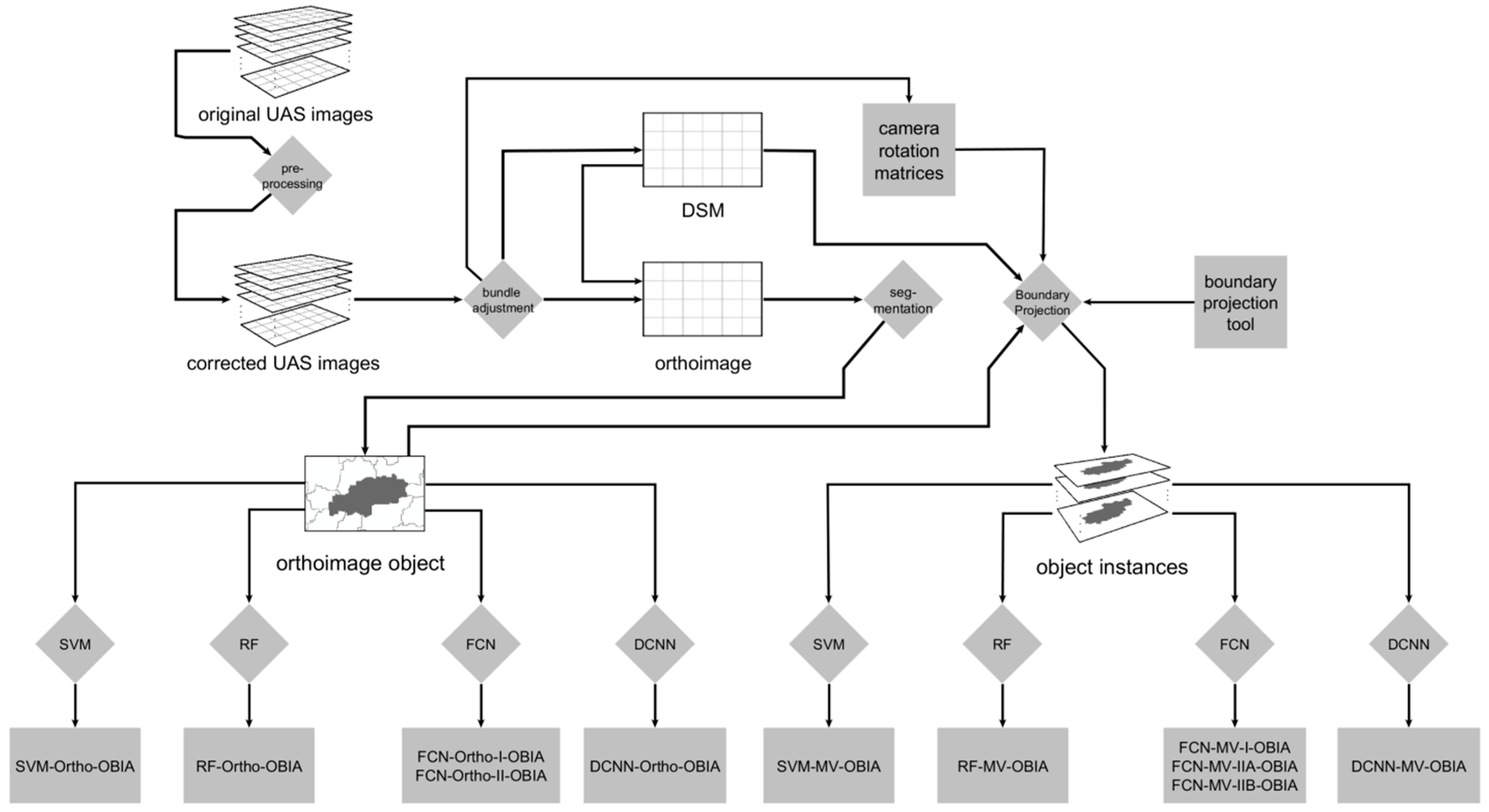
The UAS images were pre-processed to correct for the change in sun angle during the acquisition period before the orthoimage is created. Given an original UAS image i with zenith angle θ i , the original UAS images was corrected as I m g C o r r e c t e d i = I m g O r i g i n a l i ( cos ( θ i ) cos ( 75 ° ) ) [47]. The operation was conducted on all of the UAS images. Once the images are corrected, the Agisoft Photoscan Pro version 1.2.4 software was used to implement the bundle block adjustment on a total of 1397 UAS images of the study area. The software was used to produce and export a 3 band (Red, Green, and Blue) 6cm resolution orthoimage, a 27 cm Digital Surface Model (DSM), and the camera exterior and interior orientation parameters.
The three-band RGB orthoimage, together with the DSM, was analyzed using object-based analysis techniques.
The Trimble’s eCognition software was used to segment the orthoimage image. Segmentation parameters the scale (50), shape (0.2) and compactness (0.5) parameters were carefully and manually selected such that they gave visually appealing segmentation results across the majority of the orthoimage following the common practice for selecting segmentation parameters for OBIA [48]. This process resulted in 40,239 objects within the study area.

3. Methods

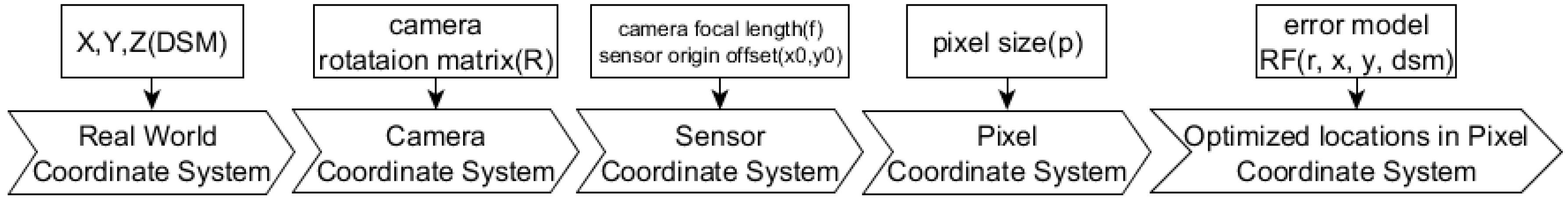
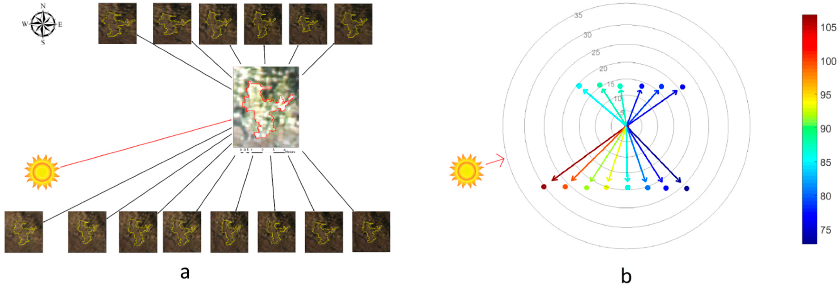
3.1. Multiview Data Generation

Given an orthoimage object, the objective of this section is to show how to generate object instances on the UAS images corresponding to this orthoimage object, to support multi-view object-based classification. This problem can be boiled down to projecting each of the vertices on the orthoimage object boundary onto UAS images. After the vertex projection is done, an object instance on the UAS image can be easily formed by threading together the projected boundary vertices. The technique introduced in this section (i.e., project a ground point onto UAS images) will be also used in Section 3.3 to generate multi-view training samples.
Given the real-world coordinates, X and Y, and Z of an object boundary vertex (or a point on the ground) on the orthoimage and the output of the bundle block adjustment results of the UAS images that were represented by the camera exterior orientation and self-calibration parameters, it is required to find the x and y coordinates (or row and column numbers) in the UAS image pixel coordinate system, if the boundary point exists on that UAS image. This requires converting XYZ from real-world coordinate system to camera coordinate system using Equation (1), followed by the conversion from camera coordinate system to sensor coordinate system by Equation (2) and then from camera sensor system to pixel coordinate system by Equation (3). However, due to the potential error coming from inaccuracies of the DSM used to extract Z value, camera parameters (e.g., focal length, pixel size) and camera lens distortion, a simple consecutive application of Equations (1)–(3) usually gave larger error. To reduce such error, we developed a two-step optimization method to reduce the projection error. The step-one is to apply the Generalized Pattern direct Search (GPS) algorithm [49] to optimize the camera parameters (e.g., focal length, sensor size, and sensor origin). The step-two is to apply random forest algorithm to model the relationship between the error and the point locations causing the error (e.g., distance from the point to UAS image center, Z value of the point and relative location of the point to the image center in terms of row distance and column distance). Average error around 1.6 pixels in the row direction and 1.8 pixels in the column direction were achieved using this method. Given the optimized camera parameters, the procedure to derive the point coordinate on UAS image is shown in Figure 2.
[ X c Y c Z c ] = [ X X 0 ,   Y Y 0 ,   Z Z 0 ] × [ r 11   r 12   r 13 r 21   r 22   r 23 r 31   r 32   r 33 ]
where X c , Y c , Z c are output of this conversion, representing point coordinates in Camera Coordinate System, X ,   Y ,   Z represent point coordinate in World Coordinate System, X 0 ,   Y 0 ,   Z 0 represent camera coordinates in World Coordinate System and r i j is the   i t h row and j th column the element of camera rotation matrix R. X ,   Y ,   Z were extracted from ArcMap using segmented orthoimage and DSM. X 0 ,   Y 0 ,   Z 0 and rotation matrix R were extracted from bundle adjustment package, such as Agisoft.
[ x s y s ] = [ x o f X c Z c y 0 f Y c Z c ]
where x s ,   y s are outputs in this conversion, representing point coordinates in Sensor Coordinate System and f is the focus length of camera. X c , Y c , Z c come from Equation (1). x o , y o are sensor coordinate offset with unit of millimeter, and they are about half of width and length of sensor dimension. f , x o , y o were also extracted from bundle adjustment result.
[ x p y p ] = [ r o u n d ( x s p ) r o u n d ( H y s p ) ]
where x p , y p are outputs in this conversion representing column number and row number of the point (i.e., raw pixel coordinates) on the UAV image taken by the camera under consideration. x s , y s come from Equation (2). p is the pixel size in millimeter and H is the height in pixels of UAV image (3456 in the case of this study). Since integer is not guaranteed as a result of division operation, the rounding operation follows.
In our study, segmentation results that were generated from eCognition package (see Section 2.3) were imported into ArcGIS to extract the vertices for each object and XYZ world coordinates of each vertex, after which vertices were then exported from ArcGIS to Matlab to generate the multi-view object instances.

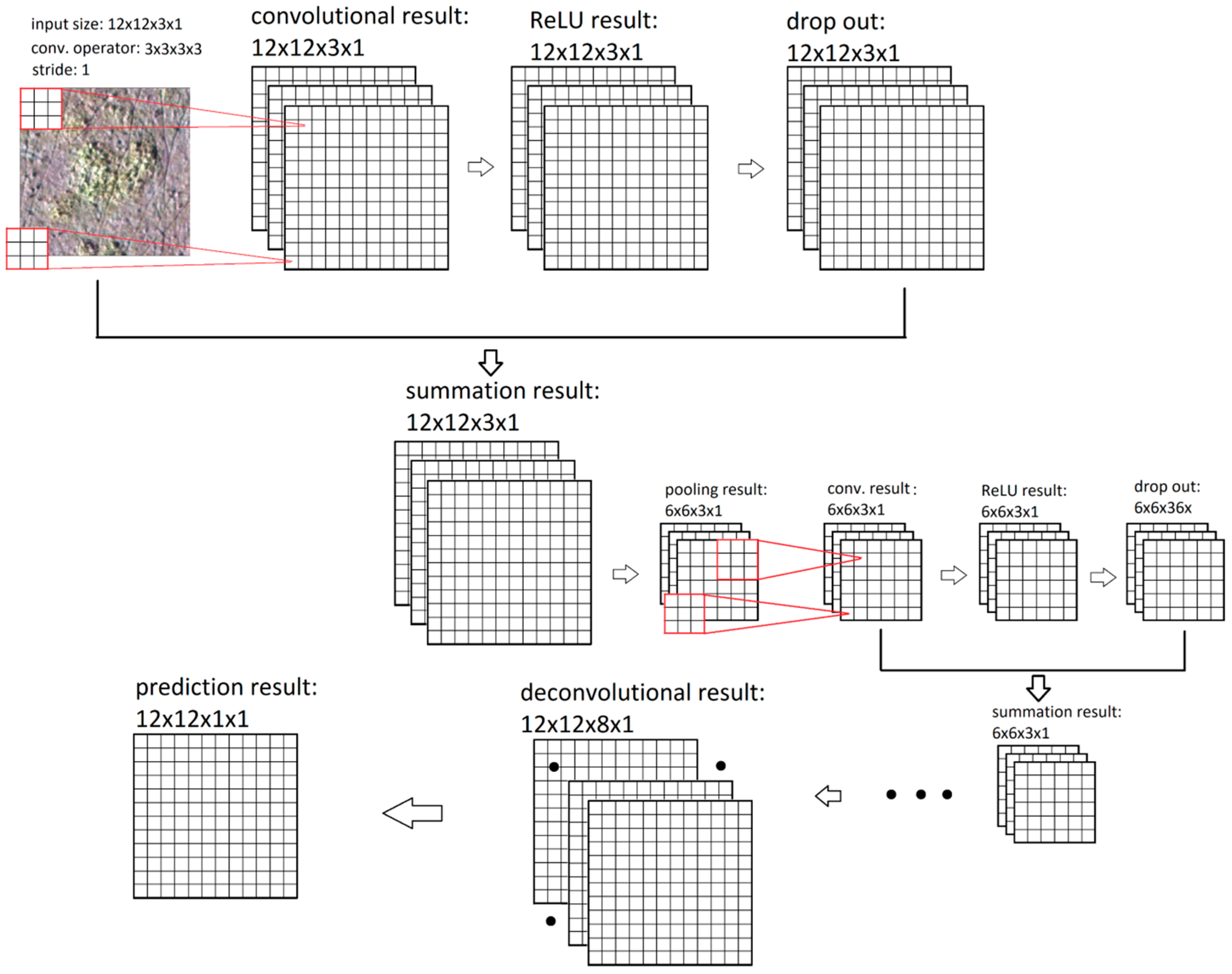
3.2. Fully Convolutional Networks

The building structure of FCN is shown in Figure 3, including the convolutional operation, regularization dropout method [50], Rectified Linear Unit (ReLU) activation function [51], summation operation [24], max pooling, and deconvolutional operation [35]. Deconvolutional operation is the key to implement the FCN and differentiate itself from the DCNN. It employs the upsampling method to turn a coarse layer into a dense layer to make the final prediction output having the same row number and column number as the input image, as indicated by the ending illustration of Figure 3.
The FCN calculates the cross-entropy for each pixel and sum them up across all of the pixels and all the training samples in a training batch as the cost.
C = 1 i = 1 n r o w i c o l i i = 1 n p = 1 r o w i q = 1 c o l i j = 1 m ( 1 { 1 } ( y p , q j ) ln ( a p , q j ) )
where, 1 A ( x ) = { 1   i f   x A 0   i f   x A , A is a given set, a p , q j = e z p , q j k = 1 m e z p , q k , n is the total number of training samples in a given training batch, m is the total number of classes, equal to 7 for our study, a p , q j is the softmax output for a row p and column q pixel location for class j training sample i, which is omitted in the notation for simplicity, y p , q j ∈ (0,1) indicating whether the ground truth class ID for a pixel located in row p and column q is j (1 means true and 0 means false).
Training of FCN is conducted through stochastics gradient descent (SGD) [52]
w u p d a t e d = w c u r r e n t λ C w
where w u p d a t e d is the updated parameter value, w c u r r e n t is the current value, λ is the learning rate, and C w is the gradient of w (i.e., derivative of parameter w) when cost value is C for a batch of training samples.
The parameter derivatives are obtained by alternatively conducting forward propagation (Equation (6)) and backward propagation (Equations (7) and (8)).
y l = h ( y l 1 )
C y l 1 = k = 1 n C y k l y k l y l 1
C w l = k = 1 n C y k l y k l w l
In Equation (6), y l and y l 1 represent variable values in layer l and l 1 , respectively, connected with function h (x):= y l 1 y l . y k l is the kth element in layer y l , through which element in y l 1 has an impact on cost C. The function h ( x ) can be convolutional operation, ReLU activation, max pooling, dropout, deconvolutional operation, and sum operation, depending on the layer type used in the FCN structure. Equation (8) does not apply to every type of layer, since some layers may not have parameters to learn, e.g., ReLU, max pooling, sum operation etc. For those layers, only Equation (7) is used during the back propagation.

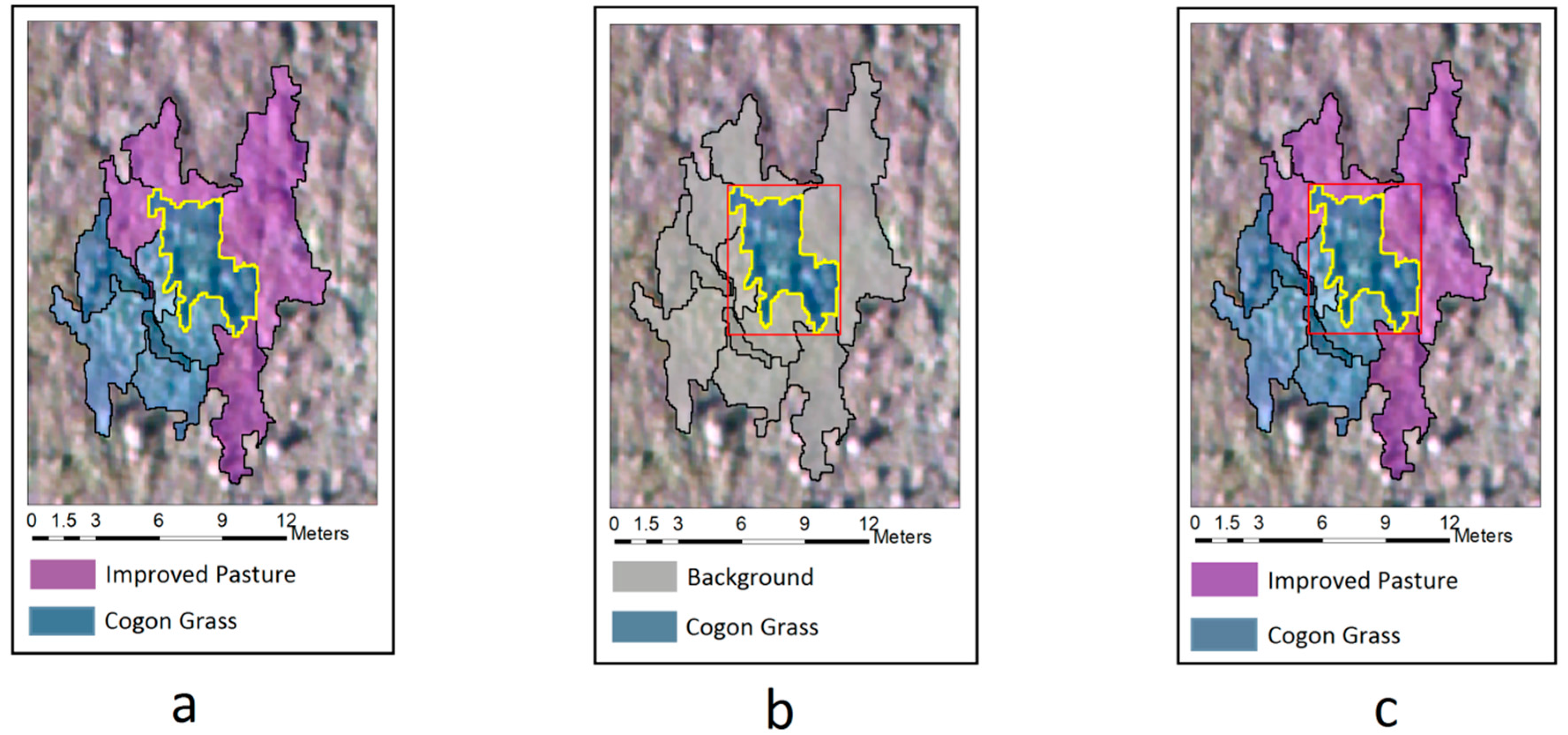
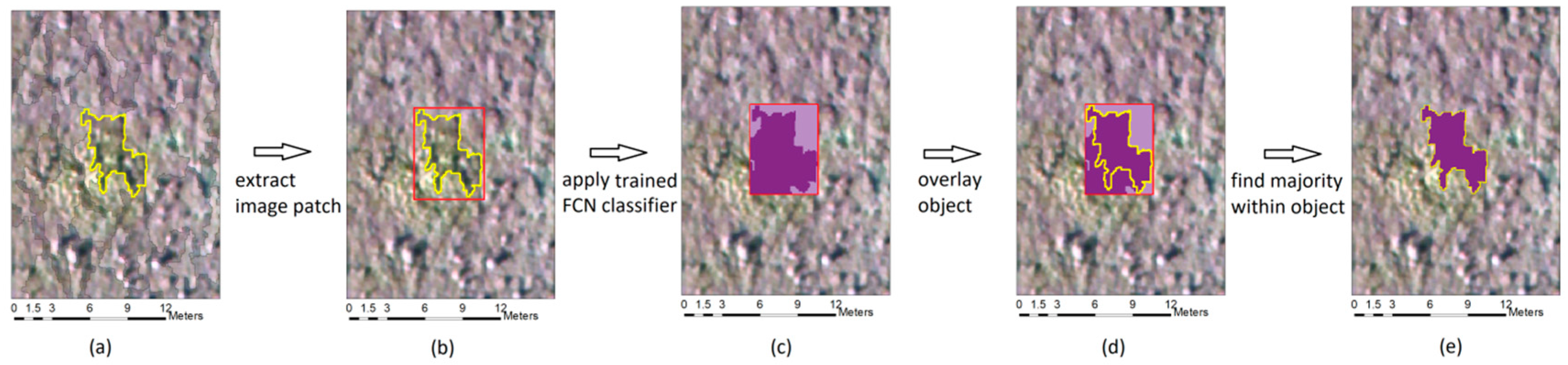
3.3. OBIA Classification Using Orthoimage with FCN

Before introducing the multi-view OBIA using FCN in Section 3.4, OBIA using orthoimage only with FCN as classifier is briefly explained in this section. Readers are referred to [25] for more details about this method. The workflow of traditional object-based image classification, commonly applied to high-resolution orthoimages, as implemented in the Trimble’s eCognition software [53] can be summarized in three main steps: (1) Image segmentation into objects using a predefined set of parameters, such as the segmentation scale and shape weight, (2) Extraction of features, such as mean spectral band values and the standard deviation of the band values for each object in the segmented image, and (3) Train and implement a classifier, such as the support vector machine [54], random forest [55], or neural network classifiers [56].
Like traditional OBIA classification, OBIA with FCN starts with orthoimage segmentation. However, different from traditional OBIA classification, a training sample for FCN is composed of an image patch and a corresponding pixel label matrix of the same size, instead of an object feature and its corresponding label in traditional object-based classification. Two options for generating the individual pixel labels of the image patch exist resulting from different treatments of the pixels surrounding the object under consideration. The first option (Option I) is to disregard the true class types for all of the pixels surrounding the object within the image patch by labeling them simply as background, while the second option (Option II) is to label each pixel with their true class types. Figure 4 illustrates these two options for creating FCN training samples for OBIA. In Figure 4a, the polygon highlighted at the center represents one sample object resulting from the orthoimage segmentation and Figure 4b,c illustrate Option I and II for preparing FCN training samples, respectively. In Figure 4b, a red rectangle is formed exactly enclosing the object; within this rectangle, only the central object pixels have true class label, while all the remaining pixels are labeled as background. In contrast, Figure 4c shows an image patch where all of the pixels inside the patch are labeled with their true class types. The Option I and II orthoimage training samples are referred to as Ortho-I and Ortho-II hereinafter.
Subsequently, FCN-Ortho-I-OBIA is used to refer to the OBIA classification using the Ortho-I (i.e., Figure 4b) training samples and FCN as classifier, while FCN-Ortho-II-OBIA is the same as FCN-Ortho-I-OBIA except that the Ortho-II (i.e., Figure 4c) sample dataset was used to train the FCN classifier.
After the FCN classifier was trained using either the Ortho-I or II training samples, the procedure that is illustrated in Figure 5 is used to generate a class label for a given object. In Figure 5, an object is highlighted at the center (Figure 5a) and a rectangle is formed enclosing it to extract the image patch (Figure 5b). Then, the trained FCN classifier is applied to the image patch to get the class labels for all of the pixels within the image patch (Figure 5c). After that, the object boundary is overlaid on the image patch again (Figure 5d) to find the majority of labeled pixels within the object as the final classification result for the object (Figure 5e).

3.4. OBIA Classification Using Multi-View Data with FCN

The multi-view data derived from the method explained in Section 3.1 is illustrated in Figure 6. At the center of Figure 6a, an object resulting from the orthoimage segmentation procedure is shown. Surrounding the orthoimage object are the UAS images with the boundary of the object instances highlighted. The figure also shows the location of sun. The variation of the automatically expanded the training dataset not only comes from geometric changes (i.e., shape distortion), but also from the spectral difference resulting from the BRDF properties of the land cover classes (see Figure 6b). It can be seen in Figure 6b that the images closer to the sun tend to have a brighter tone. The phenomenon can be attributed to the “hotspot” effect of the BRDF [57]. To make this phenomenon appear more obvious, the mean value of red band for each object instance on the UAS image is calculated and plotted on a concentric diagram in Figure 6b, where warmer color indicates a higher digital number value and zenith values are represented by circles every 5° from 5° to 35°. The projection, as shown in Figure 6a, was implemented using techniques introduced in Section 3.1. Subsequently, the object on the orthoimage that is located at the center of Figure 6a is referred to as orthoimage object, while the objects on the UAS images surrounding the orthoimage object in Figure 6a are referred to as multi-view object instances.
To implement the OBIA classification using multi-view data with FCN, training was first performed using multi-view training samples, instead of orthoimage training samples (i.e., Ortho-I and II training samples shown in Figure 4). This way, training samples were expanded to 10–14 times the training samples that were used in the OBIA relying on the orthoimage only, when considering that one orthoimage object may generate 10–14 object instances on the UAS images, as indicated in Figure 6a. After FCN was trained using the expanded (multi-view) training samples, the same procedure illustrated in Figure 5 was applied to each of the multi-view object instances. After classification results for all of the multi-view object instances were obtained, voting was conducted to find the majority vote as the final classification result for the orthoimage object.
The multi-view training samples version corresponding to Ortho-I and Ortho-II were referred to as MV-I and MV-II, respectively, hereafter. The objective is to automatically generate MV-I and MV-II given label information on the orthoimage, avoiding the laborious work to prepare training samples for multi-view classification. Such an automation procedure is critical for performing multi-view classification using FCN from a practical point of view since training samples for the multi-view classification are 10–14 times the orthoimage objects and preparing such a large number training samples manually is tedious and time-consuming. The methods proposed in this study to automatically generate MV-I and MV-II training samples are explained in the following:

3.4.1. Multi-View Training Samples without Context Information (MV-I Sample Generation)

Given an Ortho-I training sample, the boundary of the object corresponding to the Ortho-I was projected onto the UAS image. Then, the MV-I training sample was generated automatically by simply labeling the pixels within the boundary with the object class label and labeling the pixels outside the boundary as background.

3.4.2. Multi-View Training Samples with Exact Context Information (MV-IIA Sample Generation)

The situation becomes more complicated when trying to automatically generate the MV-II training sample since it requires the labelling of all of the pixels using their true class types. This study proposed and compared two methods for generating MV-II samples, and they are referred to as MV-IIA and MV-IIB, respectively. While MV-IIA samples are exact reproductions of labelling information based on the orthoimage samples, MV-IIB, with an approximate copy of labelling information, is also introduced due to its simplicity and comparable classification performance compared with MV-IIA. Each of these two methods (MV-IIA and MV-IIB) are explained below.
Given one orthoimage object with the ground truth label information, as shown at the center of Figure 7a, MV-IIA generation starts with projecting to the UAS images some vertices selected (referred to as the VS set, hereafter) surrounding the orthoimage object, after which training sample on the orthoimage were reconstructed on UAS images using the label information of these projected vertices in VS. VS should be carefully selected: the number of vertices in set VS should be high enough to allow accurate labelling of each pixel within the image patch used as FCN input, while at the same time, it should be low enough to facilitate fast projection computation.
In this study, we propose the method illustrated in Figure 7 to select the VS vertices. The object that is highlighted in Figure 7a (orthoimage object) is surrounded with labeled objects of Improved Pasture class and Cogon Grass class. The black dots in Figure 7a represent the vertices of the object boundary, noting that these vertices are shared by neighboring objects. In Figure 7b, a series of object bounding boxes (enclosing rectangles) were generated by rotating the object’s bounding box on the orthoimage around the orthoimage object every 4.5 degrees to account for the possible rotations of the object on the UAS images. In Figure 7c, the area that is covered by all bounding boxes (with all rotations) was extracted. In Figure 7d, a two-pixel wide buffer area is created to account for the potential distortion of the bounding box resulting from the distortions expected in aerial imagery, including the effect of the projective projection. Then, the vertices in Figure 7a that were coincident with the shaded area in Figure 7e were extracted. Those selected vertices shown in Figure 7e, make up all the vertices in VS. Finally, these vertices shown in Figure 7e were projected onto the UAS images to reproduce the MV-IIA.
After the vertices in the VS were projected from the orthoimage onto the UAS image, they were used for reconstructing the training samples on the UAS images. It should be noted that there is a many-to-many relationship between objects and vertices, so that one vertex may be shared by multiple neighboring objects and one object contains multiple vertices. To take advantage of this relationship for generating the multi-view training samples more efficiently, we built a simple relational database, as shown in Figure 8, so that for any central object (or its neighboring objects) within an orthoimage patch projected on the UAS images, we can easily determine which vertex it contains and what class label it belongs to and vice versa.
The vertices within the projected image patch were extracted, denoted as VSp. Clearly, VSp ⊆ VS, since VSp corresponds to one fixed orientation, while VS was extracted from virtually 360-degree orientation. We queried the database to find all of the object IDs corresponding to the vertex in VSp and we denote the found object IDs as set C. For each of the elements in C, we queried the database again to find all the vertex belonging to this element and the class ID corresponding to the object. After that, a closed boundary was created based on the found vertices and the found class ID is assigned to the closed area bounded by these vertices and patch boundaries. We repeat this procedure for all the element in C to fill the projected patch with its associated class labels. This labeled image patch makes up one training sample for the multi-view FCN classification.

3.4.3. Multi-View Training Samples with Approximate Context Information (MV-IIB Sample Generation)

As we just showed, MV-IIA requires the implementation of vertex determination (see Figure 7) and relational database (see Figure 8), not only for the sample object, but also for surrounding objects to accurately label each pixel within the image patch on each UAS image having the sample object. This is a complicated process demanding expensive computations. To simplify the procedure, we designed another method that uses nearest neighborhood method to approximate label information for the MV-II samples. The samples that were generated using this method is denoted as MV-IIB samples.
The method used to prepare the MV-IIB samples is illustrated in Figure 9, which shows an orthoimage training sample on the left (Figure 9a) and one multi-view training sample that is automatically generated using the nearest neighborhood labeling method on the right (Figure 9b). It should be noted that in practice the multi-view sample may be rotated as compared to the orthoimage object, but for illustration purposes, we let the multi-view training sample and the orthoimage sample have the same orientation in Figure 9. In Figure 9a, the two-pixel wide buffer area of the central object is highlighted in yellow. For each pixel within this yellow area, we extracted its label information from the orthoimage training sample. After the pixels within the buffer area are projected onto the UAS images, we assign the nearest neighbor label from the buffer area to the unlabeled pixels between the image patch boundary and buffer area. For the area surrounded by the buffer area, we just simply assign the label of the central object to all of the pixels within this area. While this method is much easier to implement, for objects having complicated neighborhood setup, it would result in mislabeled pixels. This imperfection is exposed by comparing the shadow area in Figure 9a,b. In the upper right corner of Figure 9b, a patch of “improved pasture” area is mislabeled as “shadow” using the nearest neighborhood labeling method, which is a recognized limitation of this method.
Following the naming conventions in Section 3.3, FCN-MV-I-OBIA is used to denote the OBIA classification utilizing the FCN classifier and MV-I training samples. FCN-MV-IIA-OBIA is the same as FCN-MV-I-OBIA, except for utilizes the IIA method to prepare the training samples. Similarly, using the MV-IIB samples produces the FCN-MV-IIB-OBIA classification results.

3.5. Benchmark Classification Methods
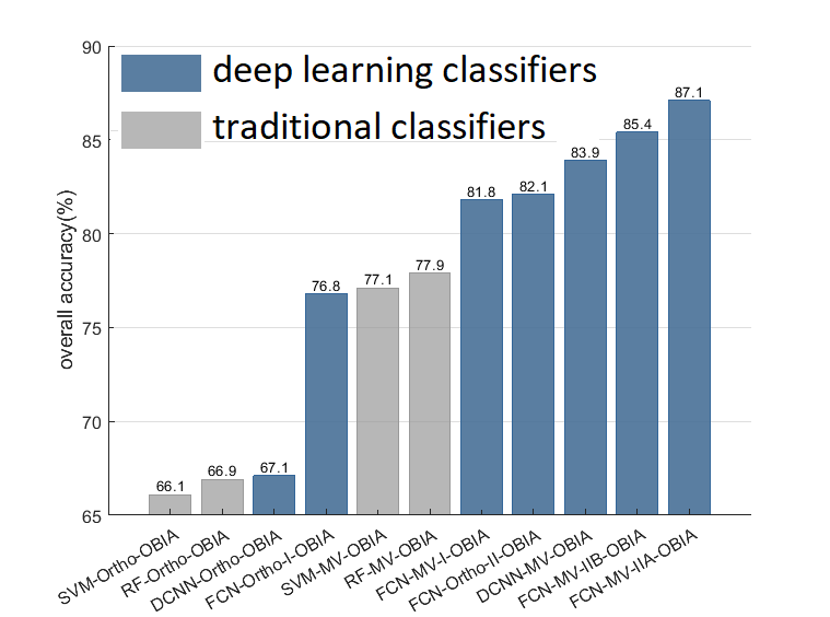
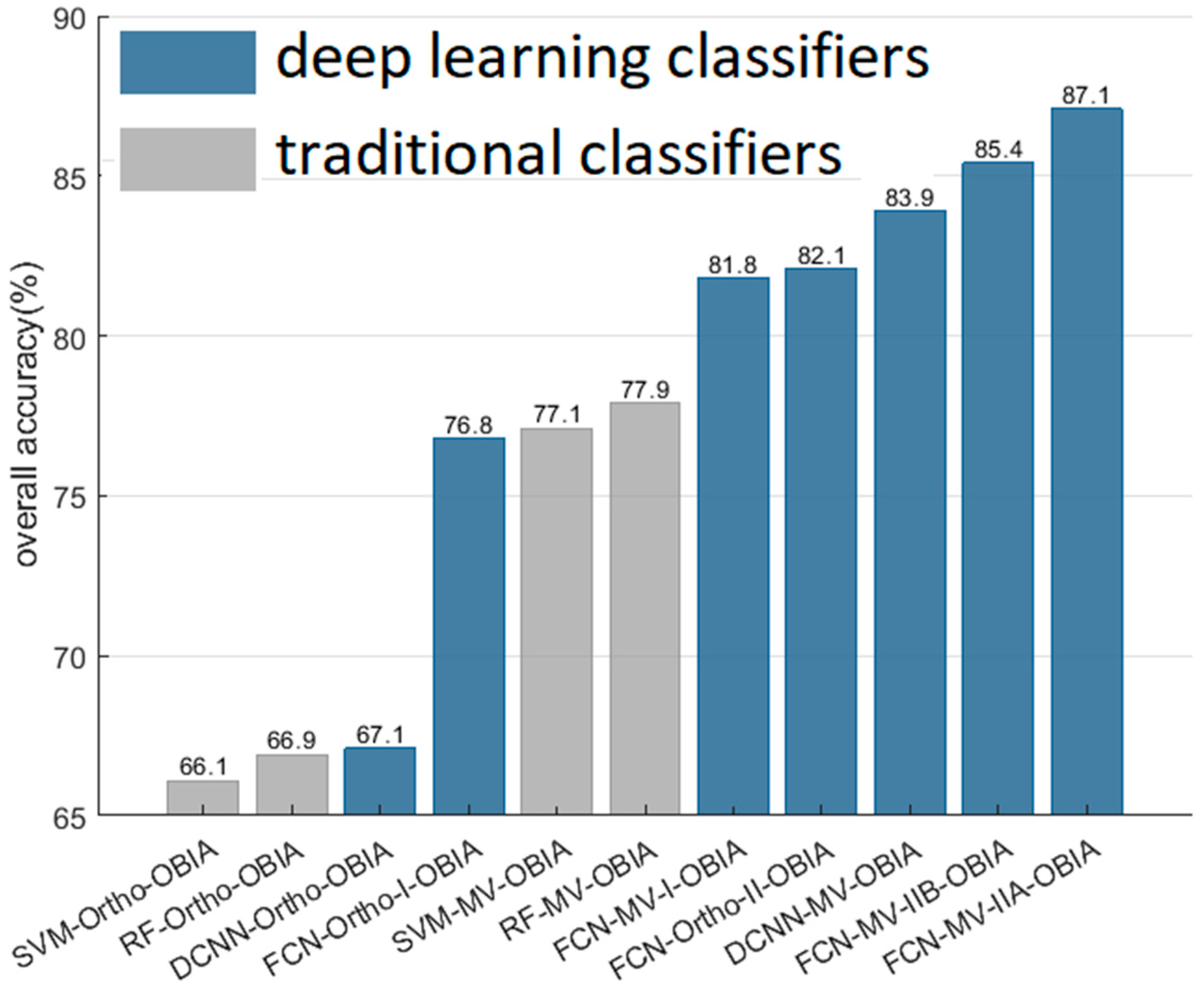
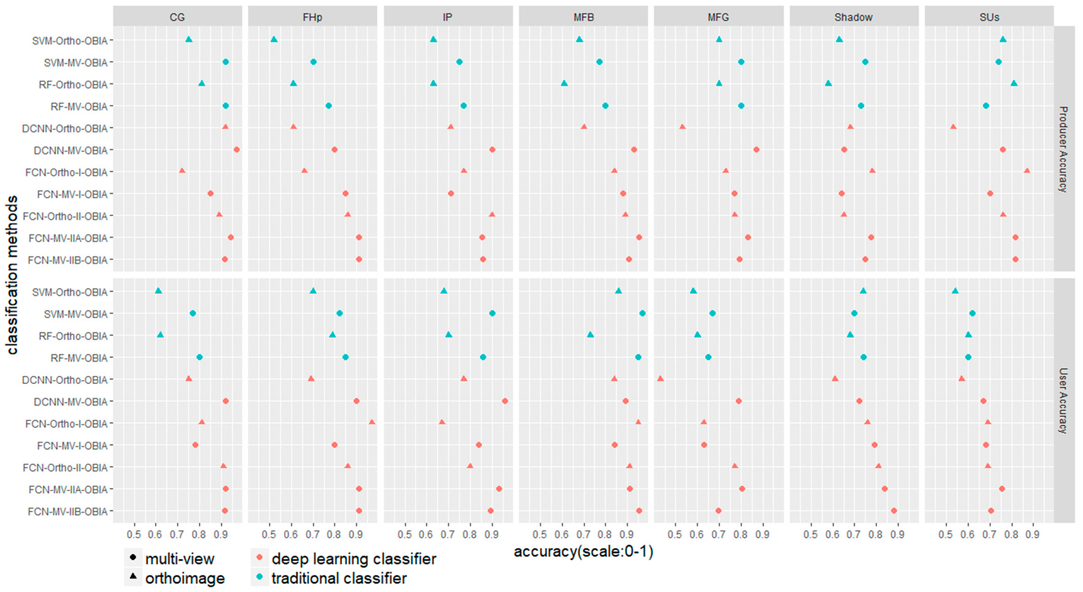
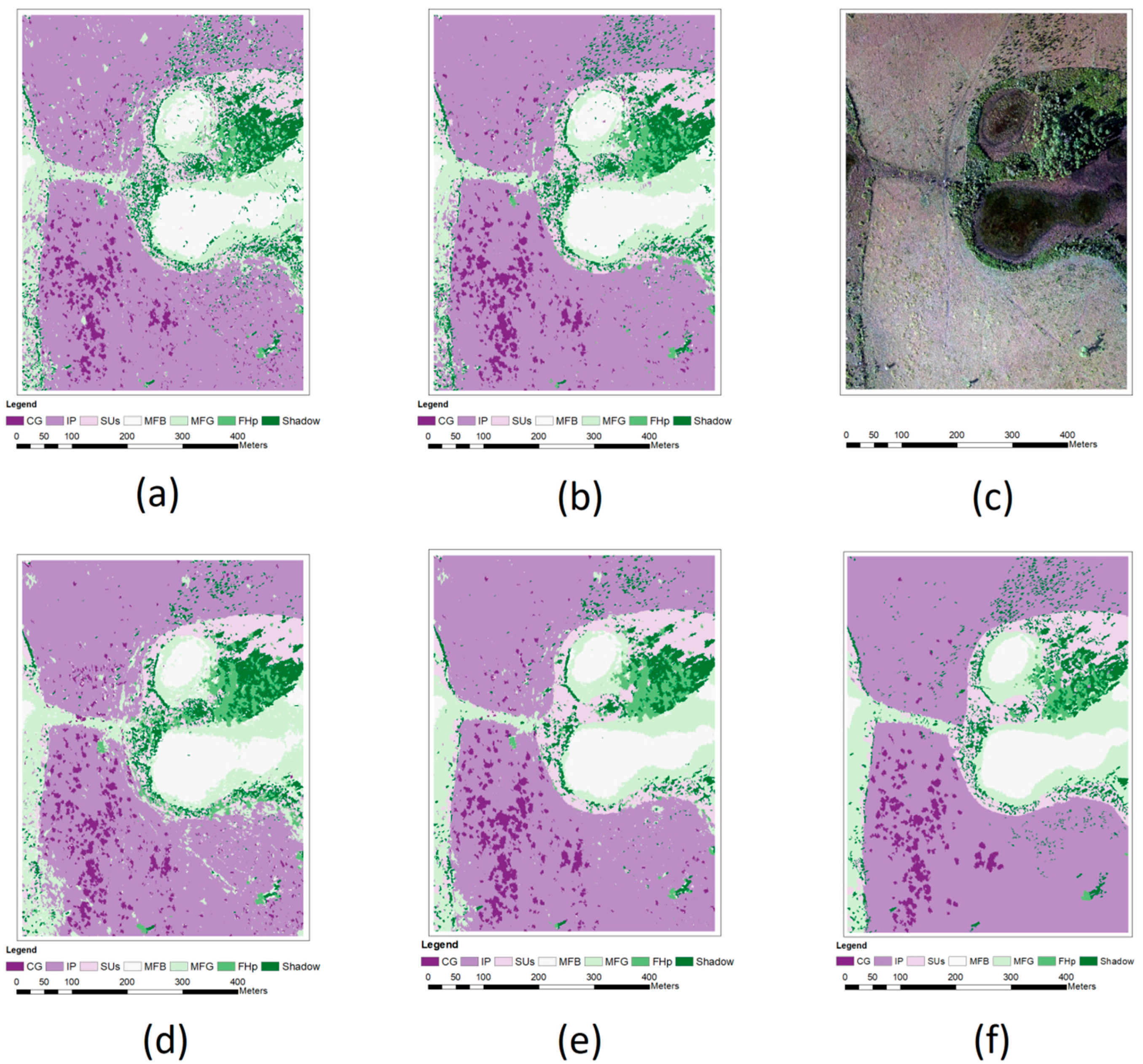
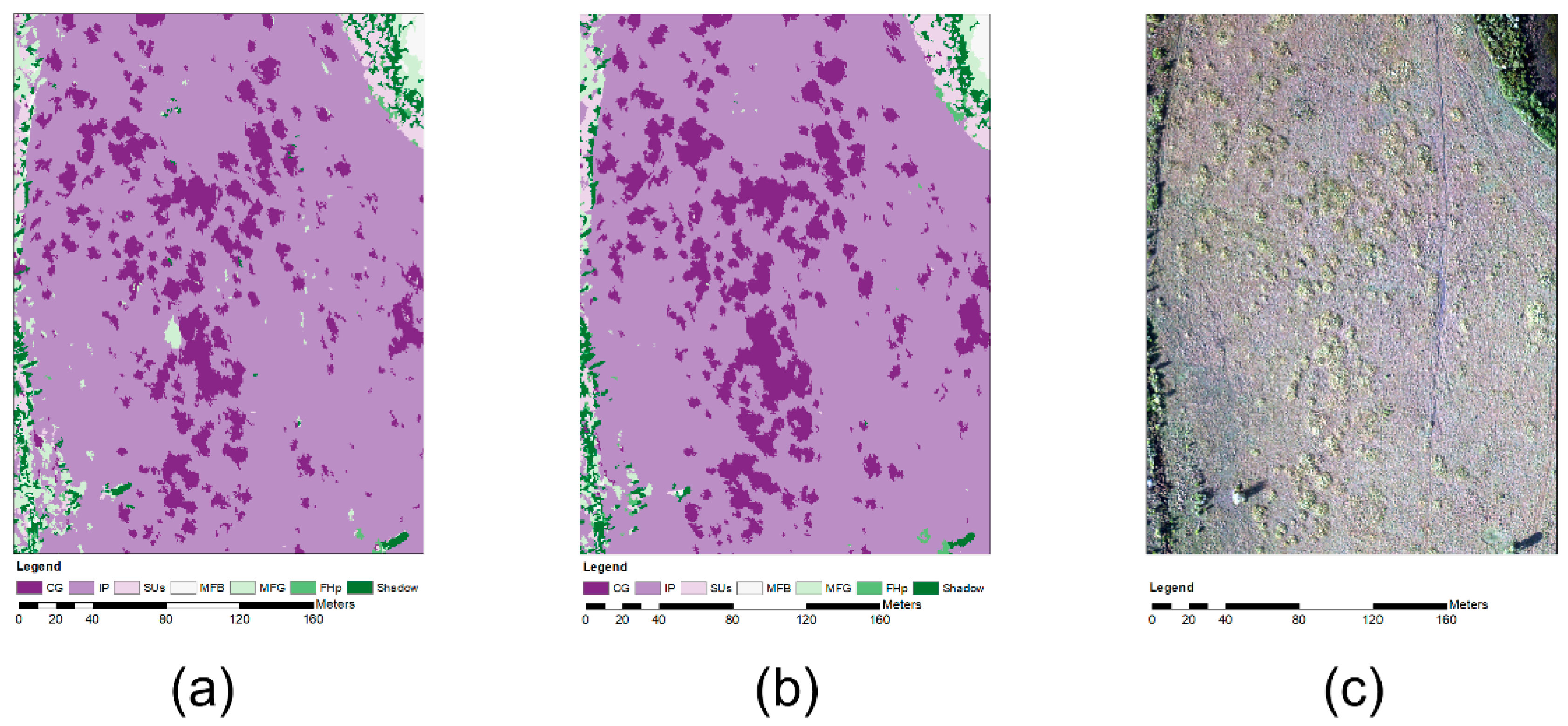
We also implemented OBIA classification using DCNN for both the orthoimage and multi-view data. The former results are denoted DCNN-Ortho-OBIA, and the latter is referred to as DCNN-MV-OBIA. Like FCN-Ortho-OBIA, DCNN-Ortho-OBIA uses image patches that exactly enclose the objects. Different from FCN-Ortho-OBIA, DCNN-Ortho-OBIA only needs label information of the central object for training, instead of all of the pixels within the image patch. DCNN-MV-OBIA obtains the final classification result for a given ground object by finding the majority vote of its multi-view object instance classification results, similar to the FCN-MV-OBIA method. The difference between DCNN-MV-OBIA and FCN-MV-OBIA is analogous to that between DCNN-Ortho-OBIA and FCN-Ortho-OBIA in terms of how the training samples are being prepared. The DCNN classifier used in this study has similar layer types as the FCN except that it does not need deconvolutional layers.
Traditional classifiers, such as Support vector machine (SVM) and random forest (RF), were tested under the OBIA framework using the orthoimage and multi-view data. The classification results utilizing orthoimage data were referred to as RF-Ortho-OBIA and the ones using multi-view data were denoted RF-MV-OBIA. Similar naming convention were applied to the SVM classification, generating the SVM-Ortho-OBIA and SVM-MV-OBIA results when using the orthoimage and multi-view data, respectively.
The RF-Ortho-OBIA and SMV-Ortho-OBIA represented the implementations of traditional OBIA classifiers as mentioned in the beginning of Section 3.3. Mean value, standard deviation, maximum, and minimum of the red, green, and blue bands were extracted and used as object features in by the RF and SVM classifiers. Gray-Level Co-Occurrence Matrix (GLCM) texture features were excluded from classification after they were tested and found having little effect on improving classification accuracy. Geometric features (e.g., object area, border and shape index features) were not included for classification, since these features were not found to be useful for OBIA classification based on our preliminary experiments and previous studies [58,59].
The same type of features was used in the SMV-MV-OBIA and RF-MV-OBIA, similar to their orthoimage counterparts. However, these features were extracted from the multi-view object instances and training was conducted using all the object instances of the training samples as done in the with FCN-MV-I-OBIA, FCN-MV-IIA-OBIA, and FCN-MV-IIB-OBIA classifications. Also, for a given orthoimage object, its final classification result was obtained by finding the majority through voting from its object instances.
The RF and SVM classifier parameters were adjusted to make sure that their performances as good as possible for our dataset. For example, the number of trees for RF was tested from 50 to 150 with 10 trees interval, with no improvement in classification accuracy when the number of trees were increased. Also, three types of kernels for SMV were tested in our preliminary experiments, and it found change of kernels from Gaussian, linear to polynomial kernels made little impact on SVM classification accuracy for our dataset. SVM is inherently a binary classifier; we adopted the one-versus-one option rather than the one-versus-all strategy to adapt for multi-class classification based on previous studies [60]. These tests resulted in using RF with 50 trees and SVM with Gaussian as kernel to generate the classification results in this study.
In summary, we experimented with 11 classification methods, including FCN-Ortho-I-OBIA, FCN-Ortho-II-OBIA, FCN-MV-I-OBIA, FCN-MV-IIA-OBIA, FCN-MV-IIB-OBIA, DCNN-Ortho-OBIA, DCNN-MV-OBIA, RF-Ortho-OBIA, RF-MV-OBIA, SVM-Ortho-OBIA, and SVM-MV-OBIA. All of these classification methods used the same set of orthoimage objects for training and testing. 400 orthoimage objects were randomly selected for each class, generating 2800 samples in total. Among the 2800 samples, 10% (i.e., 280) were randomly selected for testing and the remaining 90% (i.e., 2520) were used for training. The 2520 orthoimage objects were used to train all of the classifiers that utilized orthoimage data. 30,807 training object instances were automatically generated using boundary projection on the UAS images from the 2520 orthoimage objects and were used to train all of the classifiers that utilized multi-view data. Regardless of the training object types (i.e., orthoimage or multi-view data), all the classifiers were evaluated using 280 orthoimage objects for testing. Obviously, to evaluate the multi-view classification results, multi-view object instances corresponding to the 280 orthoimage objects were extracted and used in the classification. 3447 object instances on UAS images were extracted for the 280 orthoimage objects. For each testing orthoimage object, its label was generated via voting from its object instances for all of the multi-view classifications.
Figure 10 shows a simplified flowchart of the OBIA classification experiments that were conducted in this study. Given an orthoimage object, vertices on its boundary were projected onto UAS images to generate object instances on UAS images using DSM, data, camera rotation matrices, and boundary projection tool. The orthoimage object and object instances were used, respectively, with classifiers SVM, RF, FCN, and DCNN, resulting in 11 sets of experiment results. As shown in Figure 10:

4. Results

Figure 11 ranks the overall accuracy for all classification results presented in Figure 10 from the lowest to the highest. Both deep learning (i.e., FCN and DCNN) and traditional classifiers (i.e., SVM and RF) are highlighted. The classification accuracy obtained in this study by conventional classifiers are comparable with previous studies conducting wetland mapping using the SVM classifier [7]. The lowest accuracy of 66.1% was obtained by traditional classification SVM-Ortho-OBIA, while the highest of 87.1% was achieved by the proposed method FCN-MV-IIA-OBIA, achieving 21.0% improvement.
Regardless of using orthoimage or multi-view data, deep learning classifiers tend to show higher classification accuracy than traditional classifiers, even though the advantages vary with types of datasets and classifiers. For example, FCN-MV-IIA-OBIA got a 10.0% improvement when compared with RF-MV-OBIA using multi-view data (87.1% for FCN-MV-IIA-OBIA versus 77.1% for RF-MV-OBIA); in contrast, FCN-Ortho-II-OBIA obtained 16.0% increase when compared with RF-Ortho-OBIA using orthoimage (82.1% for FCN-Ortho-II-OBIA versus 66.1% for RF-Ortho-OBIA).
FCN produced much higher accuracy compared to the other three classifiers when all of them used orthoimage information (76.8% for FCN-Ortho-I-OBIA versus 66.1% for SVM-Ortho-OBIA, 66.9% for RF-Ortho-OBIA, and 67.1% for DCNN-Ortho-OBIA). After adding individual pixel information to FCN, it produced even higher accuracy (82.1% for FCN-Ortho-II-OBIA versus 76.8% for FCN-Ortho-I-OBIA). Multi-view data still benefitted the FCN for classification (81.8% for FCN-MV-I-OBIA versus 76.8% for FCN-Ortho-I-OBIA, 87.1% for FCN-MV-II-OBIA versus 82.1% for FCN-Ortho-II-OBIA).
Figure 12 shows the producer and user accuracy for all the 11 classification experiments. In Figure 12, deep learning classifiers (i.e., FCN and DCNN) and traditional classifiers (i.e., RF and SVM) are denoted using two different colors. Classification results using the orthoimage and multi-view data are represented by triangles and circles, respectively. It should also be noted that for a given classifier, the results of using the orthoimage and multi-view data are placed together in Figure 12 (see axis notations on the left boundary of Figure 12), with classification results of the orthoimage data always being placed above the classification using multi-view data. Figure 12 shows that with only few exceptions, multi-view classifiers tend to give higher classification accuracies than those using orthoimage data only for all classes. Additionally, deep learning classifiers tend to show higher accuracies than the traditional classifiers generally. For the invasive Cogan grass class (CG), DCNN-MV-OBIA obtained the highest producer and user accuracy, implying that this classification method is useful for mapping this invasive vegetation. While RF showed slightly better accuracy than SVM for the CG and FHp classes, these two classifiers presented comparable accuracies for other classes. FCN-MV-II-OBIA showed higher accuracy than FCN-MV-I-OBIA for all the classes except the producer accuracy of the IP class and the user accuracy of the MFG class, indicating that the object’s surrounding information benefitted the FCN classification in general. Figure 12 also indicates that hilly landscapes seem to benefit more from multi-view classification than the relatively flatten landscapes do. For example, FHp consists of various trees, resulting in more elevation variations than other landcover types in our study area, and Figure 12 shows for most classifiers the accuracy improvements due to the use of multi-view data tend to be higher for FHp class than that for other classes. This conclusion needs further investigation in a topographically rugged landscape, which can be a subject for future studies.
Figure 13 presents the classification maps that were derived from FCN, together with orthoimage and reference map. When compared with maps that are generated by the other classifiers, Figure 13e is closer to the reference map based on visual inspection, which is consistent with what we observed in Figure 11, emphasizing the superiority of the FCN-MV-IIA-OBIA classifier. Figure 13 also indicates many IP areas are mislabeled as CG in Figure 13a,d, implying the relatively high commission error (i.e., lower user accuracy) of the CG class using FCN-Ortho-I-OBIA and FCN-MV-I-OBIA, which is in line with the results in Figure 12.
Figure 14 displays the zoom-in version of Figure 13 to highlight the area impacted by Cogon grass. Figure 14b,c show the FCN-Ortho-II-OBIA and FCN-MV-IIA-OBIA having similar quality for mapping Cogon grass, reflecting similar accuracy for Cogon grass as shown in Figure 12. Notice that in the lower right corner, IP area is more easily to be flooded than other areas due to its relatively lower elevation in this wetland setup, making this small patch of IP spectrally similar to the MFG class. Such a phenomenon that different land covers may exhibit similar spectral response is not uncommon in a wetland area, as indicated in several wetland studies [61,62]. The multi-view classification approach seems more sensitive to this subtle change than their counterparts using orthoimage for classification, with more pixels of the IP class in this area being even mistakenly classified as MFG by the FCN-MV-IIA-OBIA than that by the FCN-Ortho-II-OBIA, which potentially constitutes one of reasons to account for the relatively higher producer accuracy for the IP class that was obtained by FCN-Ortho-II-OBIA shown in Figure 12.

5. Discussion

FCN showed higher accuracy than traditional classifiers (i.e., RF, SVM), regardless of whether these classifiers were applied on orthoimage data (76.8% for FCN-Ortho-I-OBIA versus 66.1% for SVM-Ortho-OBIA and 66.9% for RF-Ortho-OBIA in Figure 11) or multi-view data (81.8% for FCN-MV-I-OBIA versus 77.1% for SVM-MV-OBIA and 77.9% for RF-MV-OBIA). The improvement by FCN, when compared to RF, is more obvious than the results of the study that are presented by [41], which showed FCN producing only 1.7% improvement (88.0% for FCN versus accuracy 86.3% for RF) in an urban environment. This is in contrast with the 9.9% and 3.9% improvement shown by the present study, respectively, for the orthoimage and multi-view data. FCN even obtained comparable accuracy using orthoimage only without context information when compared with RF and SVM that used multi-view data (76.8% for FCN-Ortho-I-OBIA versus 77.1% for SVM-MV-OBIA and 77.9% for RF-MV-OBIA), which shows the relatively high efficiency of FCN in utilizing the training data for classification when compared with traditional classifiers.
In addition to its superior classification accuracy, FCN does not require feature extraction and selection. These attributes make FCN a preferred classifier over RF and SVM for OBIA classifications from a perspective of accuracy. However, it should be mentioned that training FCN is extremely slow when compared with traditional classifiers, even though applying the trained FCN to testing data is as fast as traditional classifiers. While it only took few minutes to train SVM and probably shorter time for RF, training FCN for FCN-Ortho-I-OBIA and FCN-MV-I-OIBA took about 17 and 76 h, respectively, even with a computer equipped with premium Graphics Processing Unit (GPU), like NVIDIA GPU Pascal Titan X.
While FCN obtained higher accuracy than DCNN using the Ortho-I samples (76.8% for FCN-Ortho-I-OBIA versus 67.1% for DCNN-Ortho-OBIA in Figure 11), DCNN overtook FCN when MV-I samples were used (83.9% for DCNN-MV-OBIA versus 81.8% for DCNN-FCN-OBIA), indicating that DCNN is more sensitive than FCN to the richness of training samples and multi-view extraction provides an effective avenue to enrich the training samples for improving deep learning classifier performance. This observation is consistent with the study by [25], which showed when the training sample size was increased, DCNN tended to show comparable or even slightly better results when compared to FCN.
Object surrounding information seems very useful for FCN to improve classification accuracy (82.1% for FCN-Ortho-II-OBIA versus 76.8% for FCN-Ortho-I-OBIA in Figure 11), and this advantage resulting from including the context information in training samples still hold for the multi-view case (87.1% for FCN-MV-IIA-OBIA versus 81.8% for FCN-MV-I-OBIA). Context information let FCN surpass the DCNN again regarding the classification accuracy (87.1% for FCN-MV-IIA-OBIA versus 83.9% for DCNN-MV-OBIA), implying that both training sample size and context information seem to control the relative performance between DCNN and FCN. The 3.2% classification accuracy increase from 83.9% by DCNN-MV-OBIA to 87.1% by FCN-MV-IIA-OBIA happens to be very close to the result from the study by [42], which when compared patch-based DCNN and FCN for pixel-based classification using only orthoimage and found FCN outperformed patch-based DCNN with 3.7% improvement (87.17% for FCN versus 83.46% for patch-based DCNN).
Approximate training data preparation method traded classification accuracy for implementation simplicity. Adding context information to the training data using the nearest neighborhood (MV-IIB samples) showed a lower but close accuracy when compared with the classification that used the MV-IIA training samples (85.4% for FCN-MV-IIB-OBIA versus 87.1% for FCN-MV-IIA-OBIA). This observation further confirms the impacts of including the accurate and rich context information in the training samples on improving the classification accuracy using FCN.
Our results demonstrated that inexpensive off-the-shelf camera mounted on UAS can be used to create a decent map for wetland area when the UAS images were processed using multi-view classification scheme and deep learning techniques. However, this study only employed RGB images for wetland mapping, while recent studies indicated that multispectral and synthetic aperture radar (SAR) have the potential to improve wetland classification [61,62,63,64,65,66]. Therefore, integrating the multi-view data from multiple sources into the multi-view classification scheme should be investigated, as one direction for future studies. Additionally, even though this study dealt with object-based area that can be at the square centimeters level, we do not see major obstacles for implementing the methodology developed in this study at the landscape level as long as the multi-view image can be produced. For such a purpose, it may require the remote sensing platform to operate at a much higher flight elevation.

6. Conclusions

This study proposed methods to utilize multi-view data for OBIA classification with the FCN as the classifier to investigate whether multi-view data extraction and use can improve FCN performance. It also experimented with two methods for preparing the multi-view training samples, to test if the object surroundings information would improve FCN performance. This study developed two methods to exactly and approximately label the training samples to explore the best practical methods to implement the multi-view OBIA using FCN. The study also compared the performance of FCN with other classifiers, such as the SVM, RF, and DCNN using orthoimage and multi-view data.
Our results indicated that multi-view data enabled FCN to improve classification accuracy, regardless of the used method for training data preparation. It also showed that multi-view OBIA using FCN that was trained with samples containing object surrounding information showed a much better performance than classification that used training samples without context information. In addition, our results indicated that training samples that were generated by an approximate method to label training object surroundings showed lower but comparable classification accuracy to classification that used exact object surroundings labeling method to generate the multi-view training samples. Finally, this study concludes that FCN is recommend in preference to RF, SVM, and DCNN, for OBIA using either orthoimage or multi-view data, if relatively longer training time is tolerable.

Acknowledgments

Publication of this article was funded in part by the University of Florida Open Access Publishing Fund.

Author Contributions

Tao Liu and Amr Abd-Elrahman conceived and designed the experiments; Tao Liu performed the experiments, analyzed the data and wrote the first version of the paper.

Conflicts of Interest

The authors declare no conflict of interest.

References

  1. Rango, A.; Laliberte, A.; Steele, C.; Herrick, J.E.; Bestelmeyer, B.; Schmugge, T.; Roanhorse, A.; Jenkins, V. Using unmanned aerial vehicles for rangelands: Current applications and future potentials. Environ. Pract. 2006, 8, 159–168. [Google Scholar] [CrossRef]
  2. Colomina, I.; Molina, P. Unmanned aerial systems for photogrammetry and remote sensing: A review. ISPRS J. Photogramm. Remote Sens. 2014, 92, 79–97. [Google Scholar] [CrossRef]
  3. Im, J.; Jensen, J.; Tullis, J. Object-based change detection using correlation image analysis and image segmentation. Int. J. Remote Sens. 2008, 29, 399–423. [Google Scholar] [CrossRef]
  4. Ke, Y.; Quackenbush, L.J.; Im, J. Synergistic use of QuickBird multispectral imagery and LIDAR data for object-based forest species classification. Remote Sens. Environ. 2010, 114, 1141–1154. [Google Scholar] [CrossRef]
  5. Blaschke, T. Object based image analysis for remote sensing. ISPRS J. Photogramm. Remote Sens. 2010, 65, 2–16. [Google Scholar] [CrossRef]
  6. Grybas, H.; Melendy, L.; Congalton, R.G. A comparison of unsupervised segmentation parameter optimization approaches using moderate-and high-resolution imagery. GISci. Remote Sens. 2017, 54, 515–533. [Google Scholar] [CrossRef]
  7. Pande-Chhetri, R.; Abd-Elrahman, A.; Liu, T.; Morton, J.; Wilhelm, V.L. Object-based classification of wetland vegetation using very high-resolution unmanned air system imagery. Eur. J. Remote Sens. 2017, 50, 564–576. [Google Scholar] [CrossRef]
  8. Wang, C.; Pavlowsky, R.T.; Huang, Q.; Chang, C. Channel bar feature extraction for a mining-contaminated river using high-spatial multispectral remote-sensing imagery. GISci. Remote Sens. 2016, 53, 283–302. [Google Scholar] [CrossRef]
  9. Belgiu, M.; Drăguţ, L. Random forest in remote sensing: A review of applications and future directions. ISPRS J. Photogramm. Remote Sens. 2016, 114, 24–31. [Google Scholar] [CrossRef]
  10. Cortes, C.; Vapnik, V. Support-vector networks. Mach. Learn. 1995, 20, 273–297. [Google Scholar] [CrossRef]
  11. Hinton, G.E.; Osindero, S.; Teh, Y.-W. A fast learning algorithm for deep belief nets. Neural Comput. 2006, 18, 1527–1554. [Google Scholar] [CrossRef] [PubMed]
  12. Krizhevsky, A.; Sutskever, I.; Hinton, G.E. Imagenet classification with deep convolutional neural networks. In Proceedings of the Advances in Neural Information Processing Systems, Lake Tahoe, NV, USA, 3–6 December 2012; pp. 1097–1105. [Google Scholar]
  13. LeCun, Y.; Bengio, Y.; Hinton, G. Deep learning. Nature 2015, 521, 436–444. [Google Scholar] [CrossRef] [PubMed]
  14. Hinton, G.; Deng, L.; Yu, D.; Dahl, G.E.; Mohamed, A.-R.; Jaitly, N.; Senior, A.; Vanhoucke, V.; Nguyen, P.; Sainath, T.N. Deep neural networks for acoustic modeling in speech recognition: The shared views of four research groups. IEEE Signal Process. Mag. 2012, 29, 82–97. [Google Scholar] [CrossRef]
  15. Suk, H.-I.; Lee, S.-W.; Shen, D. Alzheimer’s Disease Neuroimaging Initiative. Hierarchical feature representation and multimodal fusion with deep learning for AD/MCI diagnosis. NeuroImage 2014, 101, 569–582. [Google Scholar] [CrossRef] [PubMed]
  16. Huval, B.; Wang, T.; Tandon, S.; Kiske, J.; Song, W.; Pazhayampallil, J.; Andriluka, M.; Rajpurkar, P.; Migimatsu, T.; Cheng-Yue, R. An empirical evaluation of deep learning on highway driving. arXiv, 2015; arXiv:1504.01716. [Google Scholar]
  17. Silver, D.; Schrittwieser, J.; Simonyan, K.; Antonoglou, I.; Huang, A.; Guez, A.; Hubert, T.; Baker, L.; Lai, M.; Bolton, A. Mastering the game of go without human knowledge. Nature 2017, 550, 354–359. [Google Scholar] [CrossRef] [PubMed]
  18. Silver, D.; Huang, A.; Maddison, C.J.; Guez, A.; Sifre, L.; Van Den Driessche, G.; Schrittwieser, J.; Antonoglou, I.; Panneershelvam, V.; Lanctot, M. Mastering the game of Go with deep neural networks and tree search. Nature 2016, 529, 484–489. [Google Scholar] [CrossRef] [PubMed]
  19. Alshehhi, R.; Marpu, P.R.; Woon, W.L.; Dalla Mura, M. Simultaneous extraction of roads and buildings in remote sensing imagery with convolutional neural networks. ISPRS J. Photogramm. Remote Sens. 2017, 130, 139–149. [Google Scholar] [CrossRef]
  20. Ma, L.; Li, M.; Ma, X.; Cheng, L.; Du, P.; Liu, Y. A review of supervised object-based land-cover image classification. ISPRS J. Photogramm. Remote Sens. 2017, 130, 277–293. [Google Scholar] [CrossRef]
  21. Ma, X.; Wang, H.; Wang, J. Semisupervised classification for hyperspectral image based on multi-decision labeling and deep feature learning. ISPRS J. Photogramm. Remote Sens. 2016, 120, 99–107. [Google Scholar] [CrossRef]
  22. Makantasis, K.; Karantzalos, K.; Doulamis, A.; Doulamis, N. Deep supervised learning for hyperspectral data classification through convolutional neural networks. In Proceedings of the 2015 IEEE International Geoscience and Remote Sensing Symposium (IGARSS), Milan, Italy, 26–31 July 2015; pp. 4959–4962. [Google Scholar]
  23. Vetrivel, A.; Gerke, M.; Kerle, N.; Nex, F.; Vosselman, G. Disaster damage detection through synergistic use of deep learning and 3D point cloud features derived from very high resolution oblique aerial images, and multiple-kernel-learning. ISPRS J. Photogramm. Remote Sens. 2017. [Google Scholar] [CrossRef]
  24. Chen, G.; Weng, Q.; Hay, G.J.; He, Y. Geographic Object-based Image Analysis (GEOBIA): Emerging trends and future opportunities. GISci. Remote Sens. 2018, 55, 159–182. [Google Scholar] [CrossRef]
  25. Liu, T.; Abd-Elrahman, A.; Jon, M.; Wilhelm, V.L. Comparing Fully Convolutional Networks, Random Forest, Support Vector Machine, and Patch-Based Deep Convolutional Neural Networks for Object-Based Wetland Mapping Using Images from Small Unmanned Aircraft System. GISci. Remote Sens. 2018, 55, 243–264. [Google Scholar] [CrossRef]
  26. Marcos, D.; Volpi, M.; Tuia, D. Learning rotation invariant convolutional filters for texture classification. arXiv, 2016; arXiv:1604.06720. [Google Scholar]
  27. Zhao, W.; Du, S. Learning multiscale and deep representations for classifying remotely sensed imagery. ISPRS J. Photogramm. Remote Sens. 2016, 113, 155–165. [Google Scholar] [CrossRef]
  28. Celikyilmaz, A.; Sarikaya, R.; Hakkani-Tur, D.; Liu, X.; Ramesh, N.; Tur, G. A New Pre-training Method for Training Deep Learning Models with Application to Spoken Language Understanding. In Proceedings of the Interspeech 2016, San Francisco, CA, USA, 8–12 September 2016; pp. 3255–3259. [Google Scholar]
  29. Pan, S.J.; Yang, Q. A survey on transfer learning. IEEE Trans. Knowl. Data Eng. 2010, 22, 1345–1359. [Google Scholar] [CrossRef]
  30. Xie, M.; Jean, N.; Burke, M.; Lobell, D.; Ermon, S. Transfer learning from deep features for remote sensing and poverty mapping. arXiv, 2015; arXiv:1510.00098. [Google Scholar]
  31. Koukal, T.; Atzberger, C.; Schneider, W. Evaluation of semi-empirical BRDF models inverted against multi-angle data from a digital airborne frame camera for enhancing forest type classification. Remote Sens. Environ. 2014, 151, 27–43. [Google Scholar] [CrossRef]
  32. Su, L.; Chopping, M.J.; Rango, A.; Martonchik, J.V.; Peters, D.P. Support vector machines for recognition of semi-arid vegetation types using MISR multi-angle imagery. Remote Sens. Environ. 2007, 107, 299–311. [Google Scholar] [CrossRef]
  33. Abuelgasim, A.A.; Gopal, S.; Irons, J.R.; Strahler, A.H. Classification of ASAS multiangle and multispectral measurements using artificial neural networks. Remote Sens. Environ. 1996, 57, 79–87. [Google Scholar] [CrossRef]
  34. Longbotham, N.; Chaapel, C.; Bleiler, L.; Padwick, C.; Emery, W.J.; Pacifici, F. Very high resolution multiangle urban classification analysis. IEEE Trans. Geosci. Remote Sens. 2012, 50, 1155–1170. [Google Scholar] [CrossRef]
  35. Long, J.; Shelhamer, E.; Darrell, T. Fully convolutional networks for semantic segmentation. In Proceedings of the IEEE Conference on Computer Vision and Pattern Recognition, Boston, MA, USA, 7–12 June 2015; pp. 3431–3440. [Google Scholar]
  36. Li, S.; Jiang, H.; Pang, W. Joint Multiple Fully Connected Convolutional Neural Network with Extreme Learning Machine for Hepatocellular Carcinoma Nuclei Grading. Comput. Biol. Med. 2017, 84, 156–167. [Google Scholar] [CrossRef] [PubMed]
  37. Pei, M.; Wu, X.; Guo, Y.; Fujita, H. Small bowel motility assessment based on fully convolutional networks and long short-term memory. Knowl.-Based Syst. 2017, 121, 163–172. [Google Scholar] [CrossRef]
  38. Huang, L.; Xia, W.; Zhang, B.; Qiu, B.; Gao, X. MSFCN-multiple supervised fully convolutional networks for the osteosarcoma segmentation of CT images. Comput. Methods Programs Biomed. 2017, 143, 67–74. [Google Scholar] [CrossRef] [PubMed]
  39. Zhu, Y.; Zhang, C.; Zhou, D.; Wang, X.; Bai, X.; Liu, W. Traffic sign detection and recognition using fully convolutional network guided proposals. Neurocomputing 2016, 214, 758–766. [Google Scholar] [CrossRef]
  40. ISPRS. 2D Semantic Labeling—Vaihingen Data. 2017. Available online: http://www2.isprs.org/commissions/comm3/wg4/2d-sem-label-vaihingen.html (accessed on 8 October 2017).
  41. Piramanayagam, S.; Schwartzkopf, W.; Koehler, F.; Saber, E. Classification of remote sensed images using random forests and deep learning framework. In Proceedings of the SPIE Remote Sensing, Edinburgh, UK, 26–28 September 2016; pp. 100040–100048. [Google Scholar]
  42. Sherrah, J. Fully convolutional networks for dense semantic labelling of high-resolution aerial imagery. arXiv, 2016; arXiv:1606.02585. [Google Scholar]
  43. Marmanis, D.; Schindler, K.; Wegner, J.D.; Galliani, S.; Datcu, M.; Stilla, U. Classification with an edge: Improving semantic image segmentation with boundary detection. arXiv, 2016; arXiv:1612.01337. [Google Scholar]
  44. Grasslands, L. Blue Head Ranch. Available online: https://www.grasslands-llc.com/blue-head-florida (accessed on 1 November 2017).
  45. Holm, L.G.; Plucknett, D.L.; Pancho, J.V.; Herberger, J.P. The World’s Worst Weeds; University Press: Hong Kong, China, 1977. [Google Scholar]
  46. Rutchey, K.; Schall, T.; Doren, R.; Atkinson, A.; Ross, M.; Jones, D.; Madden, M.; Vilchek, L.; Bradley, K.; Snyder, J. Vegetation Classification for South Florida Natural Areas; US Geological Survey: St. Petersburg, FL, USA, 2006. [Google Scholar]
  47. Koukal, T.; Atzberger, C. Potential of multi-angular data derived from a digital aerial frame camera for forest classification. IEEE J. Sel. Top. Appl. Earth Obs. Remote Sens. 2012, 5, 30–43. [Google Scholar] [CrossRef]
  48. Im, J.; Quackenbush, L.J.; Li, M.; Fang, F. Optimum Scale in Object-Based Image Analysis. Scale Issues Remote Sens. 2014, 197–214. [Google Scholar] [CrossRef]
  49. Audet, C.; Dennis, J.E., Jr. Analysis of generalized pattern searches. SIAM J. Optim. 2002, 13, 889–903. [Google Scholar] [CrossRef]
  50. Hinton, G.E.; Srivastava, N.; Krizhevsky, A.; Sutskever, I.; Salakhutdinov, R.R. Improving neural networks by preventing co-adaptation of feature detectors. arXiv, 2012; arXiv:1207.0580. [Google Scholar]
  51. Nair, V.; Hinton, G.E. Rectified linear units improve restricted boltzmann machines. In Proceedings of the 27th International Conference on Machine Learning (ICML-10), Haifa, Israel, 21–24 June 2010; pp. 807–814. [Google Scholar]
  52. Bottou, L. Large-scale machine learning with stochastic gradient descent. In Proceedings of COMPSTAT’2010; Springer: Berlin, Germany, 2010; pp. 177–186. [Google Scholar]
  53. eCognition® Developer 8.8 User Guide; Trimble Documentation: Munich, Germany, 2012.
  54. Scholkopf, B.; Smola, A.J. Learning with Kernels: Support Vector Machines, Regularization, Optimization, and Beyond; MIT Press: Cambridge, MA, USA, 2001. [Google Scholar]
  55. Breiman, L. Random forests. Mach. Learn. 2001, 45, 5–32. [Google Scholar] [CrossRef]
  56. Yegnanarayana, B. Artificial Neural Networks; PHI Learning Pvt. Ltd.: Delhi, India, 2009. [Google Scholar]
  57. Kuusk, A. The hot spot effect in plant canopy reflectance. In Photon-Vegetation Interactions; Springer: Berlin, Germany, 1991; pp. 139–159. [Google Scholar]
  58. Gupta, N.; Bhadauria, H. Object based Information Extraction from High Resolution Satellite Imagery using eCognition. Int. J. Comput. Sci. Issues (IJCSI) 2014, 11, 139. [Google Scholar]
  59. Yu, Q.; Gong, P.; Clinton, N.; Biging, G.; Kelly, M.; Schirokauer, D. Object-based detailed vegetation classification with airborne high spatial resolution remote sensing imagery. Photogramm. Eng. Remote Sens. 2006, 72, 799–811. [Google Scholar] [CrossRef]
  60. Hsu, C.-W.; Lin, C.-J. A comparison of methods for multiclass support vector machines. IEEE Trans. Neural Netw. 2002, 13, 415–425. [Google Scholar] [PubMed]
  61. Mahdavi, S.; Salehi, B.; Granger, J.; Amani, M.; Brisco, B.; Huang, W. Remote sensing for wetland classification: A comprehensive review. GISci. Remote Sens. 2017. [Google Scholar] [CrossRef]
  62. Amani, M.; Salehi, B.; Mahdavi, S.; Granger, J.; Brisco, B. Wetland classification in Newfoundland and Labrador using multi-source SAR and optical data integration. GISci. Remote Sens. 2017, 54, 779–796. [Google Scholar] [CrossRef]
  63. Amani, M.; Salehi, B.; Mahdavi, S.; Granger, J.E.; Brisco, B.; Hanson, A. Wetland Classification Using Multi-Source and Multi-Temporal Optical Remote Sensing Data in Newfoundland and Labrador, Canada. Can. J. Remote Sens. 2017, 43, 360–373. [Google Scholar] [CrossRef]
  64. Rapinel, S.; Hubert-Moy, L.; Clément, B. Combined use of LiDAR data and multispectral earth observation imagery for wetland habitat mapping. Int. J. Appl. Earth Obs. Geoinf. 2015, 37, 56–64. [Google Scholar] [CrossRef]
  65. Mahdianpari, M.; Salehi, B.; Mohammadimanesh, F.; Brisco, B.; Mahdavi, S.; Amani, M.; Granger, J.E. Fisher Linear Discriminant Analysis of coherency matrix for wetland classification using PolSAR imagery. Remote Sens. Environ. 2018, 206, 300–317. [Google Scholar] [CrossRef]
  66. Wilusz, D.C.; Zaitchik, B.F.; Anderson, M.C.; Hain, C.R.; Yilmaz, M.T.; Mladenova, I.E. Monthly flooded area classification using low resolution SAR imagery in the Sudd wetland from 2007 to 2011. Remote Sens. Environ. 2017, 194, 205–218. [Google Scholar] [CrossRef]
Figure 1. Study area: left corner highlights an area seriously impacted by invasive vegetation Cogon Grass.
Remotesensing 10 00457 g001
Figure 2. Procedure to project a ground point XYZ to pixel coordinates on Unmanned Aerial System (UAS) images.
Remotesensing 10 00457 g002
Figure 3. Building structure of Fully Convolutional Network (FCN) showing the deconvolutional operation implemented to make the output having the same row and column number as the input.
Remotesensing 10 00457 g003
Figure 4. Ortho-I and Ortho-II training samples. Image patch boundary is indicated by the red rectangle: (a) Cogon grass object surrounded by Improved Pasture and Cogon Grass objects; (b) pixels within the patch surrounding the object are labeled as background for Ortho-I sample; (c) all pixels within the patch are labeled using their true class types for Ortho-II sample.
Remotesensing 10 00457 g004
Figure 5. Procedure to get the object label using trained classifier: (a) an object is overlaid on the orthoimage; (b) a rectangle is formed to extract image patch; (c) apply the trained FCN classifier to the image patch to label all the pixels within the image patch; (d) overlay the object onto the classification result; (e) find the majority of pixel labels within the object to obtain the final classification results for the object.
Remotesensing 10 00457 g005
Figure 6. Multi-view data for an orthoimage object: (a) multi-view object instances corresponding to an orthoimage object; (b) distribution of the mean value of the object’s red band for the multi-view object instances.
Remotesensing 10 00457 g006
Figure 7. Illustration to show the procedure to select vertices for projection: (a) vertices resulting from segmentation and an object under consideration highlighted at the center; (b) rotated rectangles enclosing the object; (c) area covered by all rectangles in grey; (d) area covered by all rectangles expanded by two pixels; (e) vertices selected (VS) to represent object under consideration and its neighborhood objects.
Remotesensing 10 00457 g007
Figure 8. Relational database used to label image patch of UAS images.
Remotesensing 10 00457 g008
Figure 9. Illustration for using nearest neighbor method to automatically generate the MV-IIB multi-view training samples from a given orthoimage training sample (Ortho-II): (a) an orthoimage training sample Ortho-II with two-pixel wide expansion highlighted in yellow; (b) multi-view training sample MV-IIB generated using the nearest neighbor labeling method on a UAS image.
Remotesensing 10 00457 g009
Figure 10. Simplified flowchart of this study experimental design.
Remotesensing 10 00457 g010
Figure 11. Overall accuracies obtained from the 11 classification methods tested in this study.
Remotesensing 10 00457 g011
Figure 12. Producer and user accuracies for different classification methods.
Remotesensing 10 00457 g012
Figure 13. Classification maps: (a) FCN-Ortho-I-OBIA; (b) FCN-Ortho-II-OBIA; (c) orthoimage; (d) FCN-MV-I-OBIA; (e) FCN-MV-IIA-OBIA; (f) Reference Map.
Remotesensing 10 00457 g013
Figure 14. Zoom-in area highlighting the Cogon grass area (a) FCN-Ortho-I-OBIA; (b) FCN-Ortho-II-OBIA; (c) orthoimage; (d) FCN-MV-I-OBIA; (e) FCN-MV-IIA-OBIA; (f) Reference Map.
Remotesensing 10 00457 g014aRemotesensing 10 00457 g014b
Table 1. Land cover classes in the study area.
Class IDClass NameDescription
CGCogon grassCogon grass (Imperata cylindrica) is an invasive, non-native grass which occurs in Florida and several other Southeastern US states.
IPImproved PastureA sown pasture that includes introduced pasture species, usually grasses in combination with legumes. These are generally more productive than the local native pastures, have higher protein and metabolizable energy and are typically more digestible. In our case, we also assume it is not infested by Cogon grass.
SUsSaw Palmetto ShrublandSaw Palmetto (Serenoa repens) dominant shrubland.
MFBBroadleaf Emergent MarshBroadleaf emergent dominated freshwater marsh. It can be found throughout Florida.
MFGGraminoid Freshwater MarshGraminoid dominated freshwater marsh. It can be found throughout Florida.
FHpHardwood Hammock-Pine ForestA co-dominate mix (40/60 to 60/40) of Slash Pine (Pinus elliottii var. densa) with Laural Oak (Quercus laurifolia), Live Oak (Q. virginiana), and/or Cabbage Palm (Sabal palmetto).
ShadowShadowShadow of all kinds of objects in the study area.
Table 2. Summary of sensor and flight procedure.
ItemsDescription
UAS TypeLight UAS with Fixed wing
Sensor NameCanon EOS REBEL SL1
Sensor TypeCCD
Pixel Dimension5184 × 3456
Length of focus20 mm
Sensor Size22.3 × 14.9 mm
ChannelsRGB
Takeoff time29/10/2015 16:54:51 EDT a
Landing time29/10/2015 17:49:33 EDT a
Takeoff Latitude27.22736549°
Takeoff Longitude−81.51152802°
Average Wind Speed5.1 m/s
Average Altitude302.7 m
Average Pixel Size6.5 cm
Forward overlap83%
Side overlap50%
FOV b across-track58°
FOV b along-track41°
a Eastern Daylight Time; b Field of view in degree.

