Proof of Feasibility of the Sea State Monitoring from Data Collected in Medium Pulse Mode by a X-Band Wave Radar System

Abstract

X-band marine radars can be exploited to estimate the sea state parameters and surface current. However, to pursue this aim, they are set in such a way as to radiate a very short pulse to exploit the maximum spatial resolution. However, this condition strongly limits the use of radar as an anti-collision system during navigation. Consequently, a continuous change of radar scale is needed to perform both the operations of waves and current estimations and target tracking activities. The goal of this manuscript is to investigate the possibility of using marine radar working in a medium pulse mode to estimate the sea state parameters and surface current, while assuring suitable anti-collision performance. Specifically, we compare the capabilities of the X-band radar for sea state monitoring when it works in short and medium pulse modes and we present the results of a comparison based on data collected during two experimental campaigns. The provided results show that there is good agreement about the estimation of wave parameters and the surface current field that make us hopeful that, in principle, it is possible to use the medium pulse mode to achieve information about sea state with a reasonable degradation.

1. Introduction

Marine radars are usually deployed for surveillance purposes, i.e., for the detection and tracking of targets to avoid possible collisions in shipping routes. The working frequencies for marine radars are X-band (9.4 GHz) and S-band (3 GHz), with wavelengths of about 3 cm and 12 cm, respectively.

In recent decades, X-band marine radar has been also employed as a remote sensing tool for sea state monitoring, not only on ships [1,2,3,4,5,6] but also in coastal areas [7,8,9,10,11,12,13]. The wavelength of X-band radar signal is approximatively equal to the wavelength of ripples present on the sea surface when a wind speed higher than 3 m/s is present. In this case, electromagnetic waves interact with the sea waves of similar wavelength [14] and this interaction generates backscattered radar echoes [15].

However, the use of X-band marine radar for sea wave monitoring has two main drawbacks: (i) the radar signal in X-band can be significantly attenuated by rainfall; and (ii) the effectiveness of the radar for sea state monitoring is well assessed for short range, which is not suitable for navigation purposes.

As a solution to the first drawback, the use of a S-band radar has been proposed in [16] where it has been shown that in the presence of rain, the use of a S-band radar provides performance comparable to that provided by X-band radar in terms of the significant wave height estimation. This is possible because S-band radar signal is not significantly attenuated by rain since the involved electromagnetic wavelengths are longer than those of X-band radar signals. Moreover, this implies that S-band radars can cover wide areas with a radius from 6 to 12 nautical miles.

An alternative solution for the second drawback is proposed in this paper, wherein X-band radar working in medium pulse mode is considered instead of that operating in short pulse mode.

By looking in detail, X-band marine radars operating at the two working modes radiate short and medium pulses with typical time duration of about 60 ns and 250 ns, respectively. The short pulse configuration allows sea state monitoring at a short range (up to 3 nautical miles) with a high spatial resolution (for a 60 ns short pulse, a “theoretical” spatial resolution of about 10 m is achieved). Therefore, the use of a short pulse is suitable for an accurate estimation of the sea state parameters and allows detection of sea waves with short wavelength (about 20 m). Conversely, the medium pulse configuration, whose performance in the estimation of sea state parameters is herein investigated, allows, in principle, a spatial resolution of about 40 m and thus the detection of sea waves with a minimum theoretical wavelength of about 80 m.

According to previous considerations, the choice of short or medium pulse mode is a trade-off between the counteracting aims of surveillance/navigation (long range) and sea state monitoring (short range).

The main contribution of this work is to provide a first proof of the feasibility of X-band radar in medium pulse mode for sea state monitoring. In particular, we present an analysis that permits assessment of the differences between the two pulse modes and analysis of the performance in the medium pulse system mode. This analysis is performed through a comparison of the performance achievable by means of the medium pulse mode and the short pulse mode, by processing data collected during three measurement campaigns at Cape Granitola harbor (Sicily, Southern Italy). These campaigns were carried out on 20 September 2015, 9 February 2017 and 2–3 April 2017. During these campaigns, radar datasets were collected by alternating unevenly the short pulse mode (62 datasets) and the medium pulse mode (48 datasets). The gathered datasets were processed by means of the inversion strategy presented in [1,17,18], which is based on the “Local Method” procedure [9,10]. The performance of the adopted inversion strategy has already been evaluated in short pulse mode by comparing the reconstructed bathymetric and surface current maps with the ground truth provided by in situ measurements [7,8,9,10,19]. This previous analysis corroborated reports that the method can provide robust and accurate reconstruction of the bathymetry and surface current map [8,9,10].

The paper is organized as follows. In Section 2, we describe the test site and a brief presentation of the data processing that is provided. Section 3 is devoted to the presentation of the results provided by the marine radar working in medium and short pulse modes, while a discussion about the achieved performance is given in Section 4. Conclusions end the paper.

2. Materials and Methods

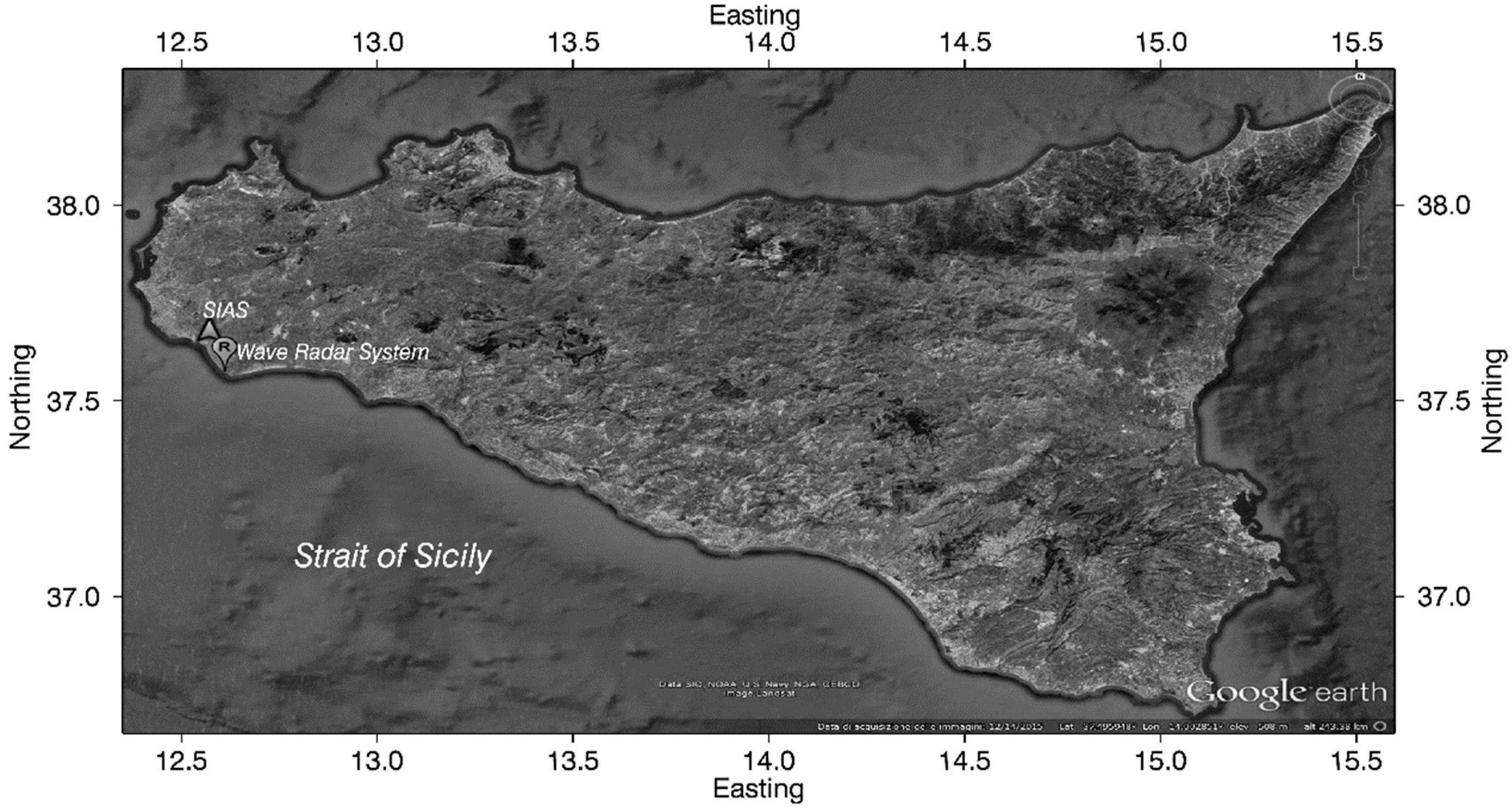
The data were collected by a wave radar system located at Cape Granitola harbor (Lat = 37°34′19.70″N; Lon = 12°39′33.45″E), in Sicily (Italy) (see Figure 1). The system was installed on an ancient water tank at the Istituto per l’Ambiente Marino Costiero (IAMC) of the Italian National Research Council (CNR), at a height of 15 m above the sea level. The marine radar is equipped with a 9 feet (2.74 m) long Consilium Selesmar antenna able to transmit electromagnetic pulses in X-band with a peak power of 25 Kw and includes an analog-to-digital (AD) converter, used for the received signal. For both pulse modes, the radar signal was acquired in polar coordinate (range, azimuth) and after was interpolated on a 1024 × 1024 pixels Cartesian grid with a pixel spacing of 4.48 m along both the spatial coordinates (Δx, Δy). The radar images were stored by using a 13-bit unsigned integer format. The single radar dataset is composed of 64 radar images collected with a time step of 2.39 s between two successive images. The time step corresponds to the antenna rotation time (Δt).

Table 1. Parameters of the radar survey.

System Parameter	Values
	Short Pulse Mode	Medium Pulse Mode
Pulse duration	60 ns	250 ns
Spatial resolution	~10 m	~40 m
Antenna rotation period (Δt)	2.39 s	2.39 s
Spatial image spacing (Δx and Δy)	4.48 m	4.48 m
Minimum range	250 m	250 m
Maximum range	2296 m	2296 m
Processed images number for a sequence (N)	64	64
Antenna height above sea level	~15 m	~15 m
View angular sector	110°	110°

summarizes the working parameters of the radar system. The estimation of the surface current and the sea-state reconstruction was achieved by means of the inversion scheme described in [7,8,9,10]. The core of the reconstruction strategy is the Normalized Scalar Product (NSP) approach [18] able to estimate the surface current and bathymetry jointly.

In particular, the NSP method is based on the maximization of the normalized scalar product between the amplitude of the radar spectrum, here denoted with $\left|F_I\left(\overline{k},\omega \right)\right|$, and the following characteristic function:

$$G\left(\overline{k},\omega ,\overline{U},h\right)=\delta \left(\omega -\sqrt{gk\tanh \left(kh\right)}-\overline{k}·\overline{U}\right)$$

(1)

which accounts for the local support of the dispersion relation. In Equation (1), $\overline{k}=\left(k_x,k_y\right)$ represents the wave vector (whose magnitude $k=\frac{2\pi }{\lambda }$ is the wave number, λ being the wavelength), ω is the angular frequency related to the wave period $T$ by $\omega =\frac{2\pi }{T}$, $g$ represents the acceleration due to gravity, h is the bathymetry value and $\overline{U}=\left(U_x, U_y\right)$ is the vector representing the sea surface current. Accordingly, the estimated $\widehat{\overline{U}}=\left({\widehat{\overline{U}}}_x, {\widehat{\overline{U}}}_y\right)$ of the surface currents are performed according to the equation:

$$\widehat{\overline{U}}=arg\underset{\overline{U}}{\max }\frac{\langle \left|F_I\left(\overline{k},\omega \right)\right|,G\left(\overline{k},\omega ,\overline{U},h\right)\rangle }{\sqrt{P_{F_I}}}$$

(2)

where $\langle \left|F_I\left(\overline{k},\omega \right)\right|,G\left(\overline{k},\omega ,\overline{U},h\right)\rangle$ denotes the scalar product between the functions $F_I\left(·\right)$, and $P_{F_I}$ denotes the power of $F_I\left(·\right)$. Let us observe that $G\left(·\right)$ has a unitary power.

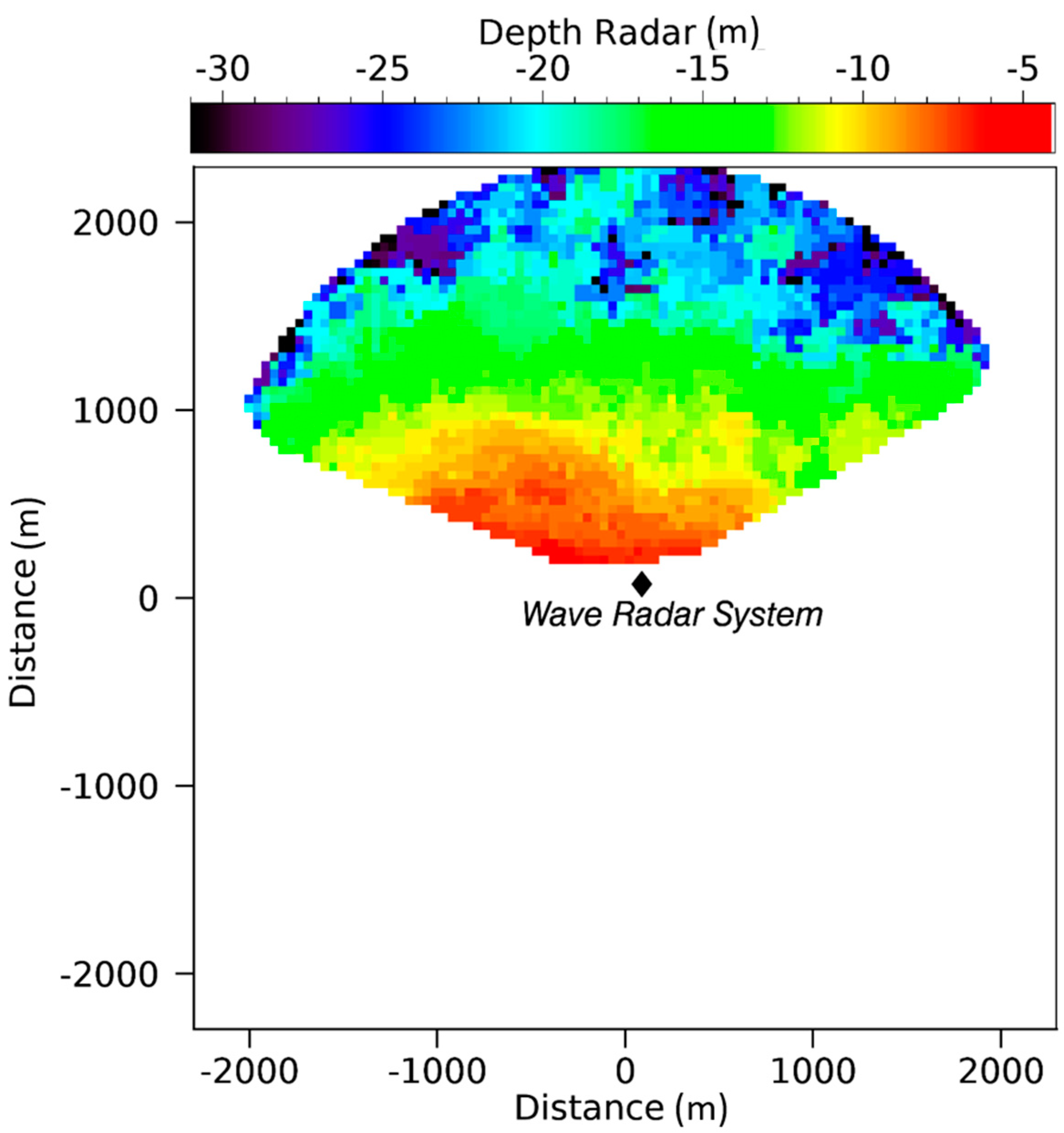
In the present work, we estimate only the surface current whereas the bathymetry of the investigate area is assumed known and provided by a previous measurement campaign [20]. The bathymetric map is depicted in Figure 2.

The knowledge of surface current is a key point in the inversion procedure to extract the linear components of the gravity waves from the image spectrum. In fact, an incorrect estimation of the sea surface current leads to an incorrect spectral filtering, with a detrimental effect on the estimation of the sea state parameters in terms of wave period, wavelength, wave direction of the dominant waves and significant wave height [18].

In [7,8], the authors proposed the “Local Method”, which improved the original version of the NSP method [18], with the aim to reconstruct spatially inhomogeneous current and sea surface current fields. Such a method relies on the spatial partitioning of the investigated region into partially overlapping patches, within which the local estimation of the surface current is performed [21].

The reconstructed sea surface current is exploited to define the Pass-Band (PB) filter, whose output is the useful sea signal cleaned by the noise, $F_{PB}\left(k_x,k_y,\omega \right)$. Afterwards, the 3D sea-wave spectrum is obtained from this filtered radar spectrum through an equalization step based on the radar Modulation Transfer Function (MTF) [17]; see Equation (3).

$$F_w\left(k_x,k_y,\omega \right)=\gamma ·MTF·F_{PB}\left(k_x,k_y,\omega \right)$$

(3)

where γ is a calibration factor, obtained by exploiting data provided by external sensor such as wave buoy, while the MTF is defined as for the sea state monitoring in the coastal area in front of Giglio Island [7,19] and reported in Equation (4).

$$MTF \propto \{\begin{array}{c}{k}^2 for k> \pi /30\\ k^{-1.8} for \pi /30\le k\end{array}$$

(4)

So, defining the MTF allows us to mitigate the distortions introduced in the radar imaging process [22,23,24,25]. It worth noting that in this measurement campaign, the same MTF has been adopted for both the working modes.

Starting from the reconstructed 3D sea wave spectrum $F_w\left(k_x,k_y,\omega \right)$, it is possible to compute the (2D) directional spectrum and derived parameters, such as: peak wavelength (λ_p), peak direction (θ_p) and peak period (T_p) of the dominant wave, and significant wave height $H_s$. In addition, the wave radar system also allows the estimation of the mean spectral parameters, such as: mean angular frequency (${\omega }_M$), mean wavenumber ($k_M$) as reported in

Table 2. Expression of the relevant mean spectra parameters.

Mean Parameters	Definitions
${\omega }_M$	$\frac{2\pi }{T_M}=\frac{{{\displaystyle \int }}_0^{2\pi }{{\displaystyle \int }}_0^{\infty }f{F}_w\left(f, \theta \right) df d\theta }{{{\displaystyle \int }}_0^{2\pi }{{\displaystyle \int }}_0^{\infty }{F}_w\left(f, \theta \right) df d\theta }$
$k_M$	$\frac{2\pi }{{\lambda }_M}=\frac{{{\displaystyle \int }}_0^{2\pi }{{\displaystyle \int }}_0^{\infty }\left|k\right|F_w\left(k, \theta \right) dk d\theta }{{{\displaystyle \int }}_0^{2\pi }{{\displaystyle \int }}_0^{\infty }{F}_w\left(k, \theta \right) dk d\theta }$
${\theta }_M$	$\arctan ({\mathrm{s}}_0/{\mathrm{c}}_0)$
${\mathrm{c}}_0$	${{\displaystyle \int }}_0^{2\pi }{{\displaystyle \int }}_0^{\infty }{F}_w\left(f,\theta \right)\cos \theta df d\theta$
${\mathrm{s}}_0$	${{\displaystyle \int }}_0^{2\pi }{{\displaystyle \int }}_0^{\infty }{F}_w\left(\mathrm{f},\mathsf{\theta }\right)\sin \mathsf{\theta } df d\theta$

. By the mean spectral parameters, the mean period (T_M), mean wavelength (λ_M) and mean direction (θ_M) can be retrieved [6]. The significant wave height $H_s$ is computed through Equation (5) [17,26].

$$H_s=4\sqrt{\underset{\overline{k},\omega }{\overset{ }{{\displaystyle \int }}}{F}_w\left(k_x,k_y,\omega \right)d{k}_{x}d{k}_{y}d\omega }$$

(5)

Finally, the spatial-temporal sea wave sequence can be reconstructed from the 3D sea-wave spectrum by exploiting the IFFT (Inverse Fast Fourier Transform) technique.

3. Results

This section presents the results obtained from the analysis of the three datasets collected on 20 September 2015, 9 February 2017, and 2–3 April 2017. The radar datasets have been acquired with a time delay of few minutes for the two working modes, and, as stated, each dataset includes 64 consecutive radar images.

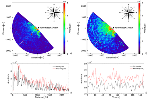
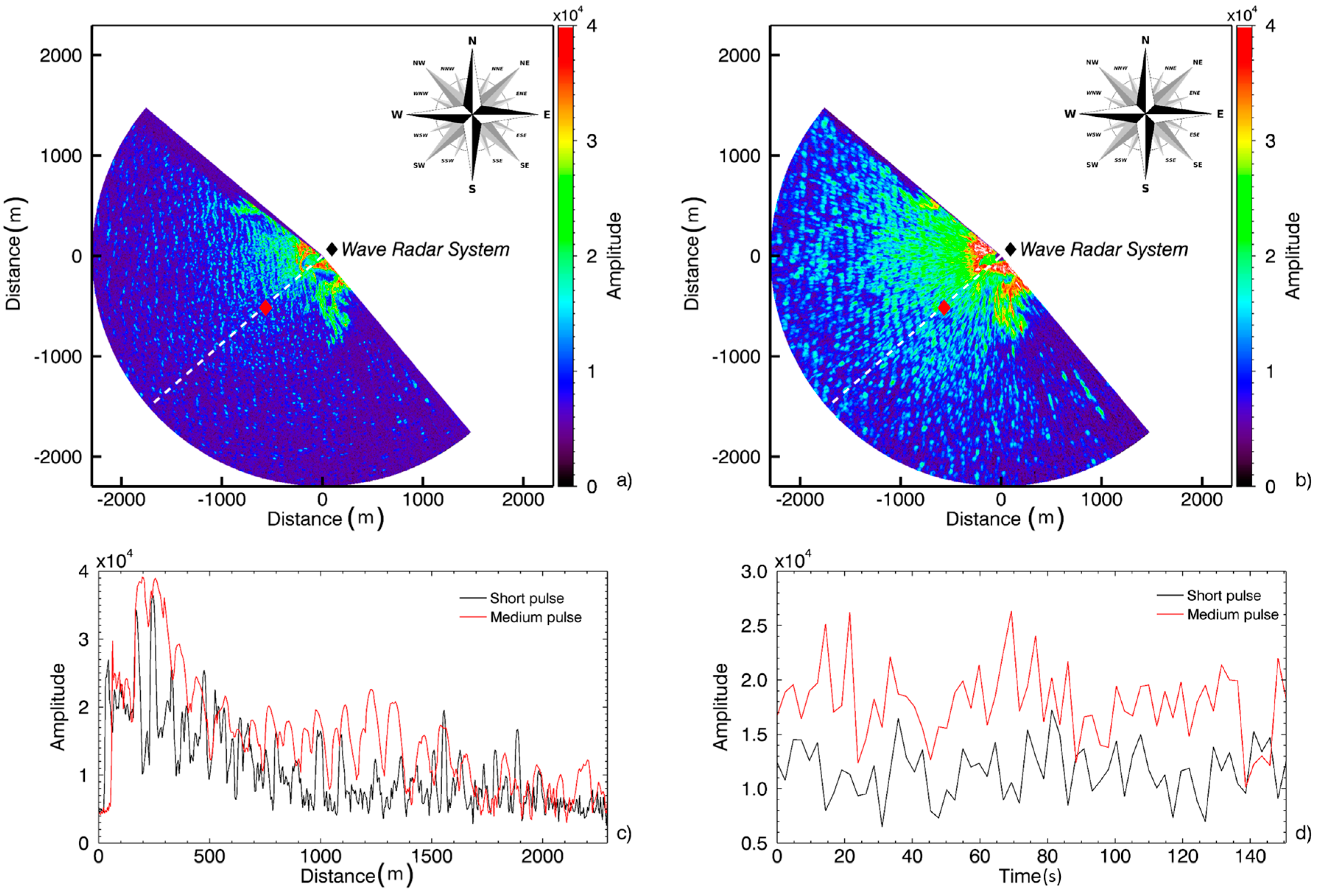
The difference between short and medium pulse modes can be observed both in the space-time domain and in the wavenumber-frequency domain; see Figure 3a,b. These figures depict a sample radar image (space-time domain) for the short and medium pulse mode, respectively, and allow us to observe a different spatial resolution. In particular, the radar image acquired with the short pulse mode (pulse duration equal to 60 ns) exhibits a range resolution of about 9 m, which increases to 35 m if the medium pulse of about 250 ns is used. In addition, Figure 3c,d compare the spatial and the temporal variation of the backscattering intensities along a transect (at a fixed time instant) and at a fixed location (at a fixed point) for two pulse modes, respectively.

Figure 4a,b depict the section of the 3D radar spectrum, along the wave propagation direction, computed from the data referring to the short and medium pulse modes respectively.

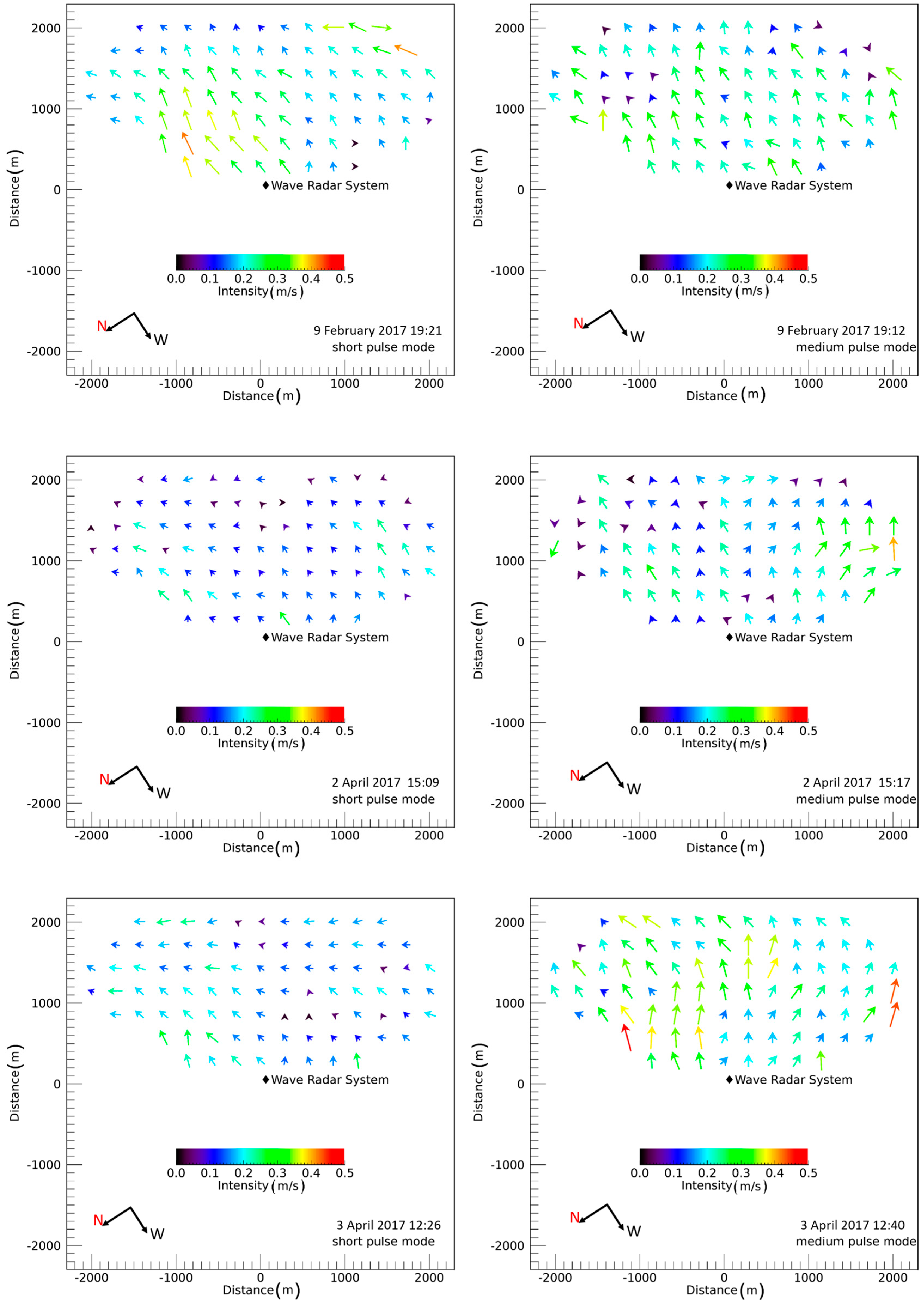
Figure 5 shows a qualitative comparison between surface current fields estimated by the data acquired in short (left panel) and medium (right panel) pulse mode (the two acquisitions are subsequent). This figure allows observation of a good agreement between the estimated of sea surface current intensity and direction provided by the two pulse modes. It is worth noting that the maps in Figure 5 are shown with respect to the radar north, which is at a 237° relative to geographic north.

To make a quantitative evaluation of the differences between the surface current fields estimated with the two different pulse lengths and shown in Figure 5, we computed the mean standard deviation (σ) and relative mean error (µ) of the intensity (I) and direction (θ) of the point-by-point difference between the surface currents maps in short and medium pulse modes. These quantities are given in

Table 3. Relative mean error and standard deviation of the intensity and direction of sea surface currents maps difference between short and medium pulse modes.

		σI	σθ	µI	µθ
9 February 2017		0.12 m/s	41.6°	0.01 m/s	4.6°
19:21 (short)	19:12 (medium)
2 April 2017		0.084 m/s	67.3°	−0.05 m/s	21.5°
15:09 (short)	15:17 (medium)
3 April 2017		0.084 m/s	59.8°	−0.1 m/s	3.7°
12:26 (short)	12:40 (medium)

.

Figure 6a,b depict the comparison of the surface current parameters in terms of mean intensity and mean direction, computed over the whole field of view, for all considered dataset. The mean current direction has been georeferenced with respect to geographic north.

Upper panels of Figure 7 show the 2D directional spectra achieved from the reconstructed sea-wave for the short (left panel) and medium (right panel) pulse mode, respectively; the comparison between the 1D frequency spectra is depicted in the bottom panels of Figure 7.

The sea state parameters, in terms of mean wave direction, mean wave period of the dominant wave, and significant wave height, estimated in both pulse modes, are shown in Figure 8, Figure 9 and Figure 10, respectively.

4. Discussion

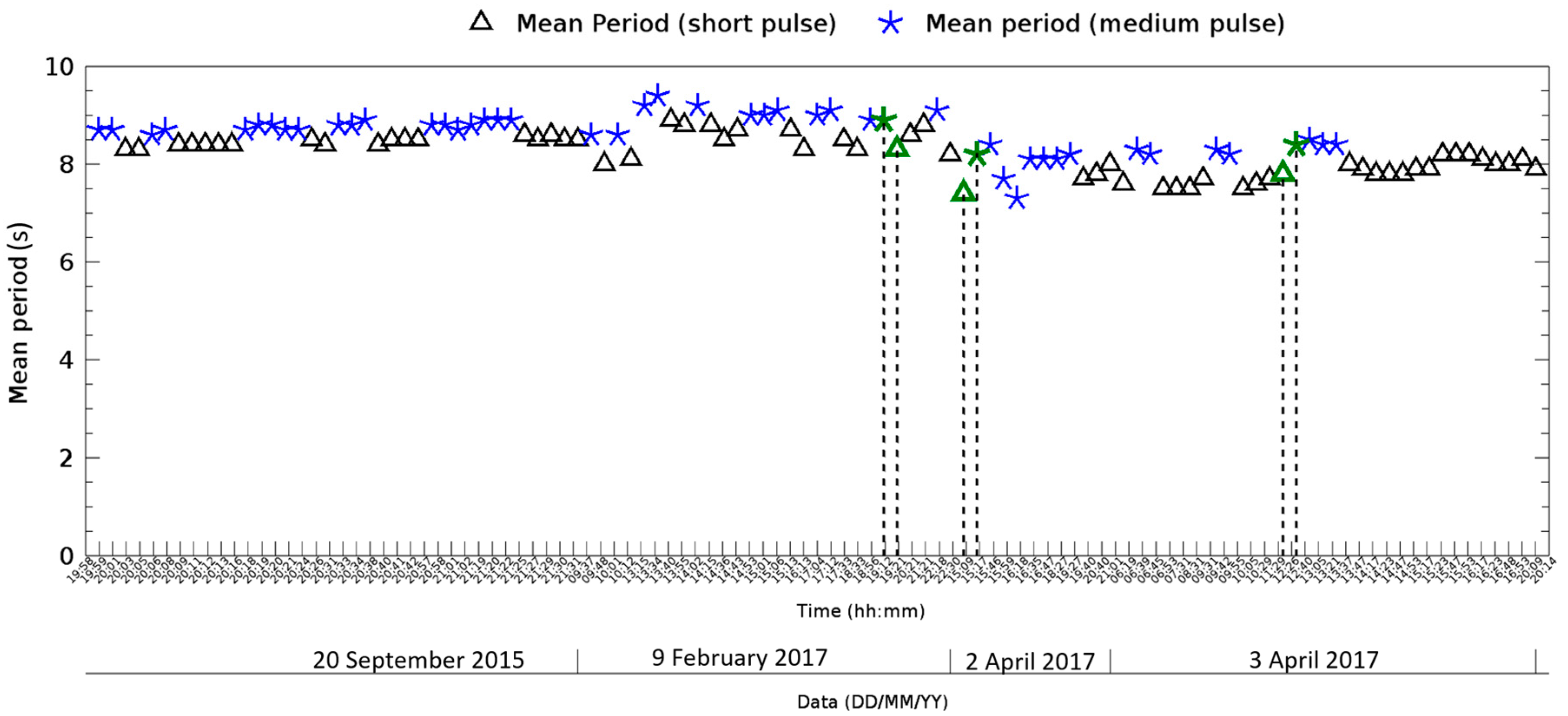
The results presented in Section 3 show that there is a good agreement between the sea state parameters estimated in short and medium pulse modes. In particular, Figure 8 and Figure 9 show that, apart from few time points, the sea state parameters, in terms of mean wave direction (θ_M) and mean wave period (T_M) obtained from the data collected by using pulse modes show the same behavior.

The main discrepancies concern the estimation of intensity and direction of the sea surface current as well as the estimation of the significant wave height (see Figure 6a,b and Figure 10). These results can be explained considering the different spatial resolution related to the two pulse modes. In fact, from the radar image shown in Figure 3b one can clearly observe that the medium pulse mode, due to the low spatial resolution, fails to discriminate sea waves when they approach the coast with respect to ones acquired in short pulse mode (see Figure 3a). This occurs because, if the water depth decreases, the interaction of sea wave with the sea bottom gives rise to an increased wave height and a decreased wavelength.

In addition, the “wave” acquired in medium pulse mode are wider and smoothed (see Figure 3c) and have larger intensity (see Figure 3d) than those referred to in the short pulse mode. Hence, the medium pulse mode is not able to capture phenomena characterized by a high spatial variability.

The above observations are coherent with the fact that, in the wavenumber-frequency domain, the relevant spectral energy of the data acquired by using the short pulse mode is spread in a wider wavenumber domain with respect to its counterpart related to the medium radar pulse (see Figure 4a,b). The absence of spectral components at high wave numbers, when the radar is configured in medium pulse mode, involves a slight over/under-estimation of the sea surface current intensity, which is comparable with the sensitivity of the wave radar (see Figure 5 and Figure 6a) [27].

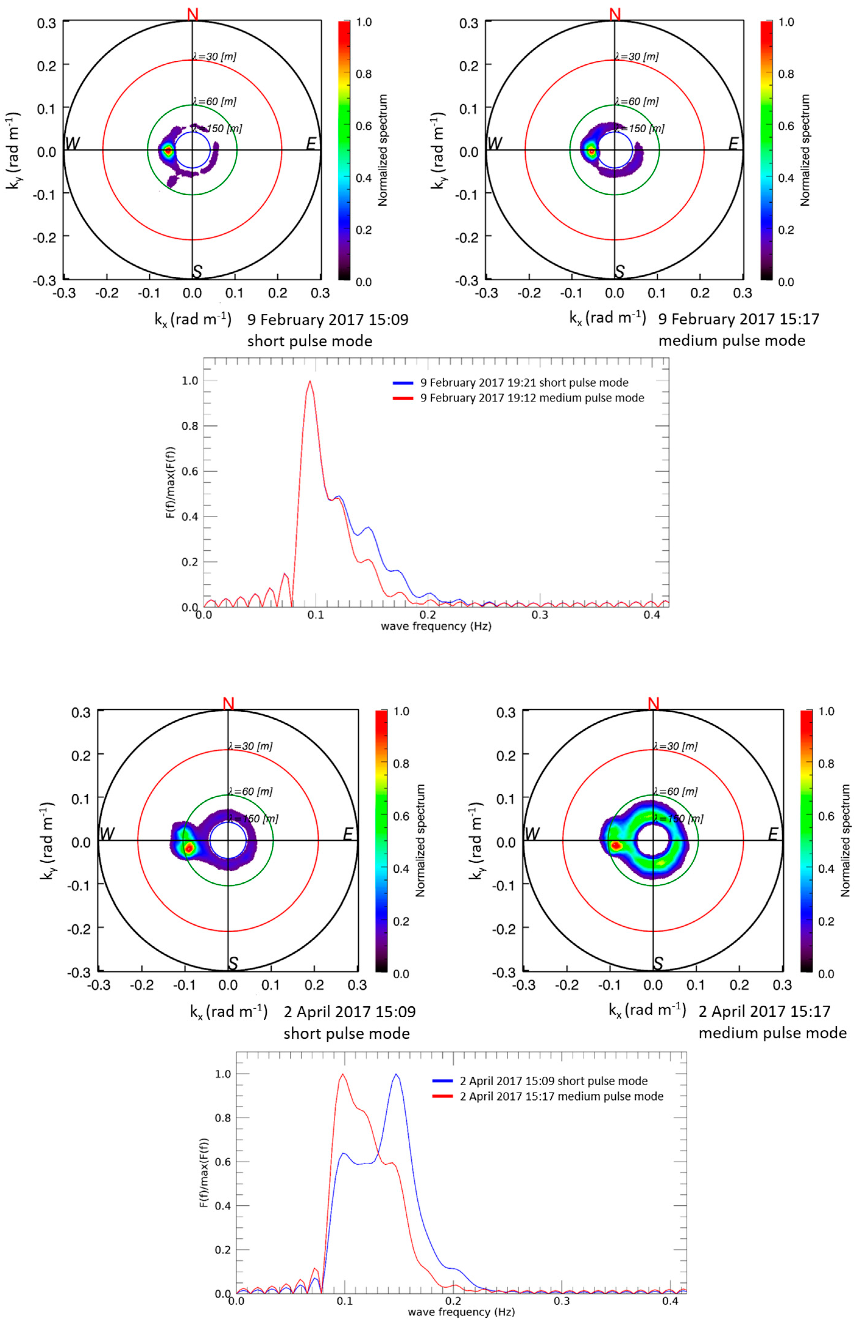
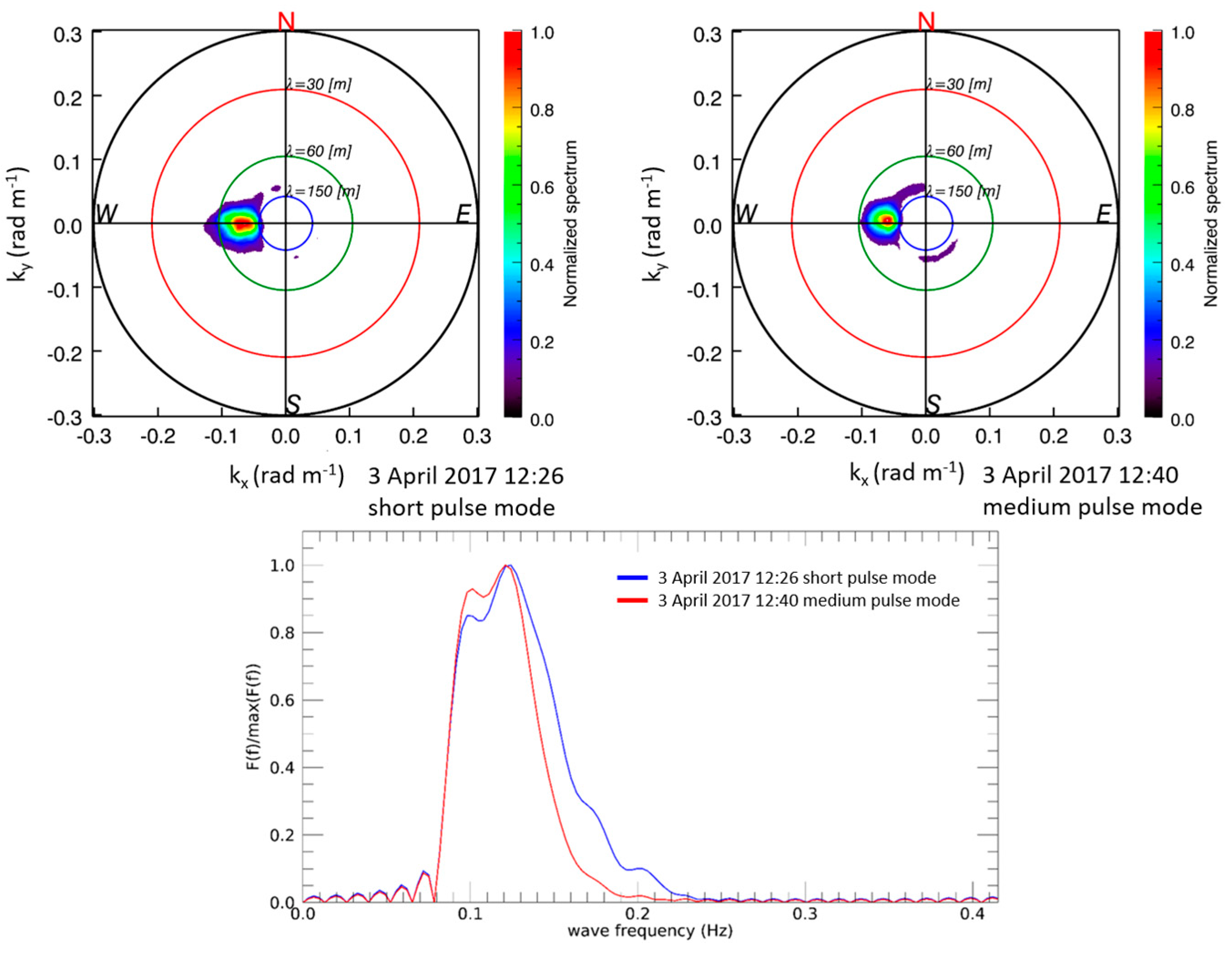
This phenomenon can be also observed both in 2D directional spectra and in 1D frequency spectra; see Figure 7. In particular, 2D directional spectra obtained in the short pulse mode have a larger bandwidth along the wavelength direction with respect to the spectra associated with medium pulse mode, while the 1D frequency spectra highlight the poor performance of the medium pulse in capturing the higher spatial variability the sea wave phenomena.

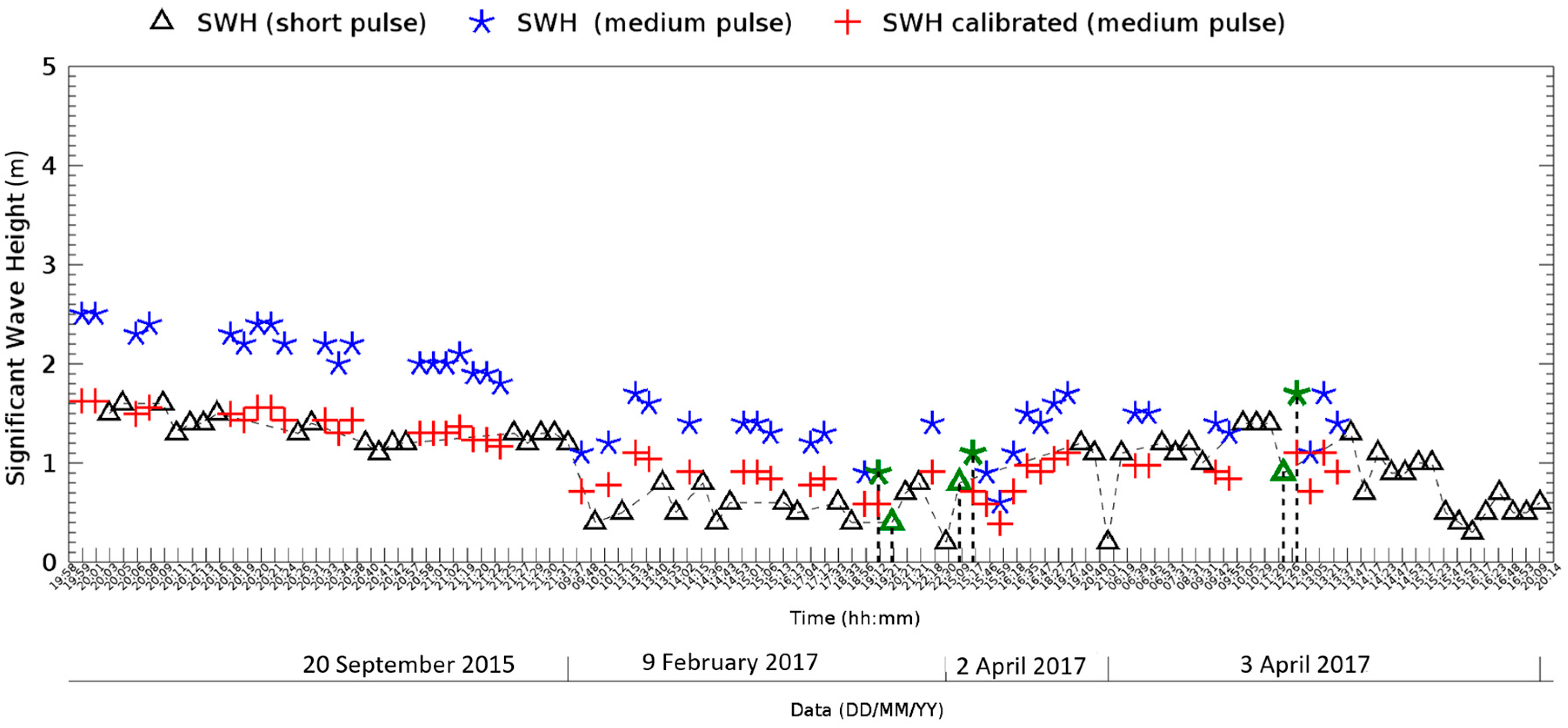
It is worth noting that the data on 9 February 2017 and 2 April 2017 have been acquired in “gentle breeze” sea conditions (Beaufort scale), i.e., significant wave height Hs < 1 m; see Figure 10. These sea conditions involve a high level of clutter in the radar images and consequently a wave spectrum power comparable to the noise spectrum power at low wavenumbers. In addition, the wave radar, installed at Cape Granitola and adopted for the presented measurement campaigns, is affected by non-appropriate tuning procedures, which degrades the radar images acquired both in medium and short pulse mode. Consequently, a greater intensity of the 2D directional spectra is possible to observe especially for the data acquired in “gentle breeze” sea conditions (see Figure 7).

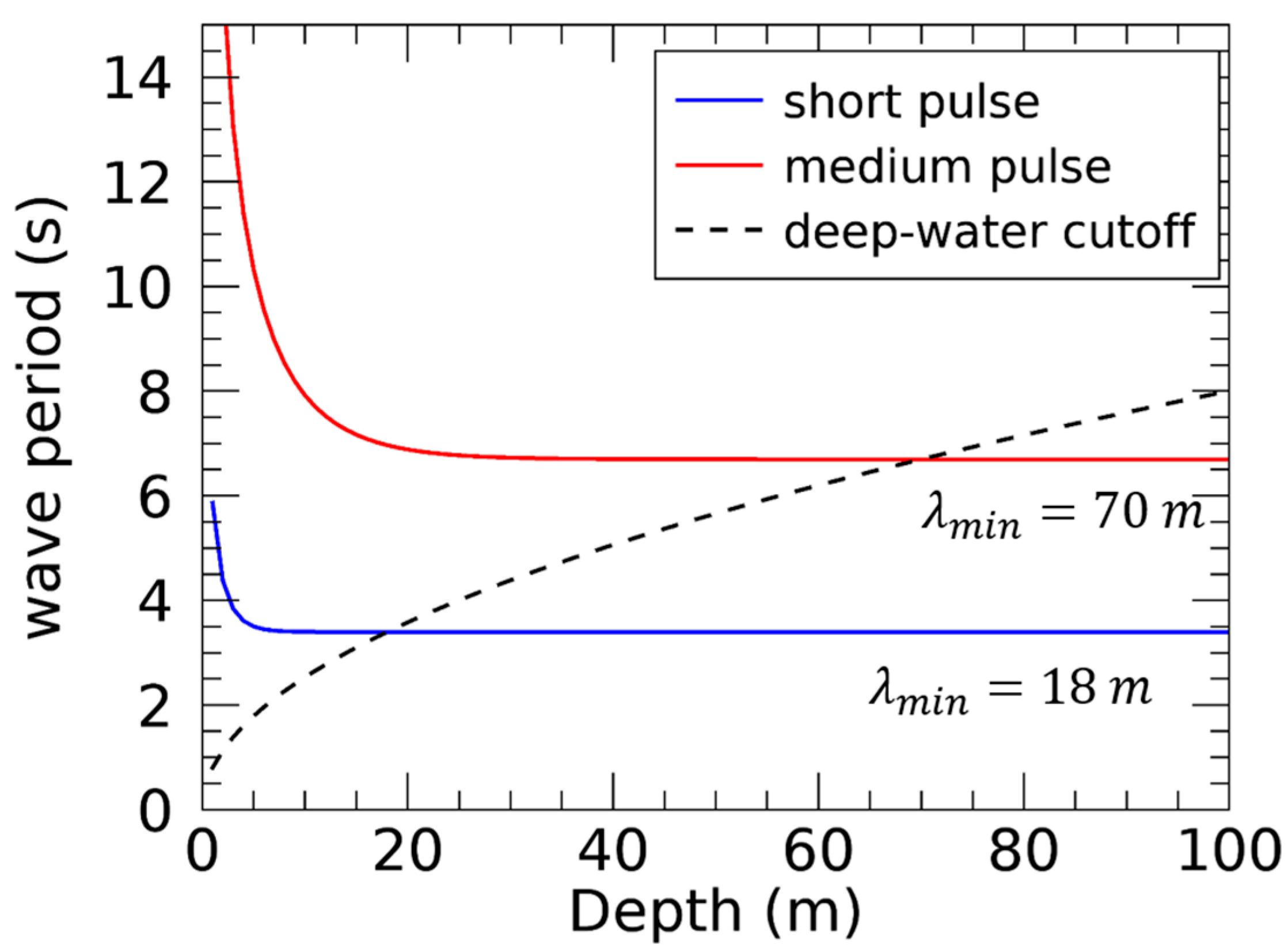
The low sensitivity of the medium pulse mode in capturing the higher spatial variability of the sea wave phenomena can be explained in term of theoretical frequency cutoff (fc) computed in the function of minimum theoretical wavelength detectable in both pulses modes. Figure 11 shows the curves of wave period (T) in the function of the bathymetry for theoretical values of minimum wavelength (λ_min) detectable in short (blue line) and medium (red line) pulse modes, together with the theoretical curve of the deep-water cutoff (black dashed line). In particular, it is possible to obtain a theoretical frequency cutoff equal to fc = 0.29 Hz (T = 3.4 s) and fc = 0.14 Hz (T = 7.1 s) for the short and medium pulse mode, respectively. Consequently, the medium pulse mode has a low sensitivity for detecting sea state with wave period lower than of 7 s.

Before discussing the discrepancy concerning the significant wave height $H_s$, it is worth noticing that the radar image, acquired by the wave monitoring system, is not the direct representation of the sea surface due distortion occurring in the electromagnetic scattering phenomenon. In particular, the intensity of the received signal is mostly related to the electromagnetic backscattering of the sea surface rather than to the sea wave elevation [17,23]. Accordingly, the function $F_w\left(k_x,k_y,\omega \right)$ retrieved from the analysis of the radar data represents a “scaled version” of the actual sea wave spectrum. Therefore, a calibration stage is required; see Equation (3).

As far as the short pulse mode is concerned, the calibration stage has already been carried out during previous campaigns [27,28]. In this paper, we use the calibration factor γ adopted in [27,28] to estimate the significant wave height $H_s$ by using both short and medium pulse modes; see Figure 10.

The two estimated $H_s$ have the same behavior, apart a multiplicative factor, and this difference is due to the different power radiated by the radar in the two considered pulse modes. In fact, the radar transmits a greater power in the medium pulse mode (see Figure 3d) and this translates into a larger radar spectrum intensity and in a larger $H_s$. This suggests the adoption of a new calibration factor for the medium pulse, which is equal to the calibration factor of the short pulse mode multiplied by a given factor. In particular, for the adopted wave radar system, this multiplicative factor is 0.65. This value has been obtained as the ratio between the mean power intensity received in short and medium pulse mode. Consequently, this calibration factor can be used for future acquisitions in medium pulse mode without a further calibration step, if the radar data acquired in the short pulse mode are available and calibrated.

Indeed, by computing in such a way γ, we achieve a good agreement between the two pulse modes, as shown by Figure 10, wherein the red crosses represent the $H_s$ values referred to the medium pulse mode with the new calibration factor.

For completeness of the results, the mean and standard deviation of all mean spectral parameters retrieved during each measurement campaign have been computed and reported in

Table 4. Mean and standard deviation of the mean sea state spectral parameters obtained for each measurement campaign.

TM (Short)	TM (Medium)	θM (Short)		θM (Medium)		Hs (Short)	Hs (Medium)
20 September 2015
Mean	9.0 s	9.0 s	266°		270°	2.3 m	2.3 m
St dev	0.2 s	0.2 s	2°		1.5°	0.2 m	0.2 m
9 February 2017
Mean	10 s	10 s	252°		261°	0.5 m	0.7 m
St dev	0.02 s	0.04 s	19°		15°	0.2 m	0.1 m
2 and 3 April 2017
Mean	8.7 s	8.6 s	262°		266°	0.9 m	0.8 m
St dev	1.1 s	1.1 s	14°		14°	0.3 m	0.2 m

.

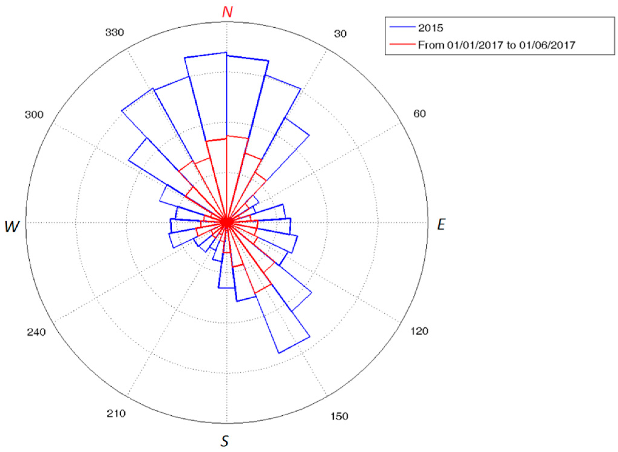
Table 4 and Figure 8 show that the mean wave direction is about 270° for all the considered period. This phenomenon can be explained by considering Figure 12, which shows the polar graphic of the density of the wind direction observed in the Cape Granitola site during the years 2015 and 2017. In fact, in this area for most part of the year, the wind blows from the NN-NW-NE (see Figure 10) and the mean wind direction differs from the direction of dominant waves due to the phenomenon of refraction, which causes rotation of about 30° to the waves that approach the coast [29]. The wind data were provided by the meteorological station of the network SIAS (Servizio Informativo Agrometeorologico Siciliano) of Mazara del Vallo, at about 13 km far from the experiment site (see Figure 1) (data available at http://www.sias.regione.sicilia.it/frameset_rete_new.htm).

5. Conclusions

In this manuscript, we have presented a proof of feasibility of sea state monitoring from data collected in medium pulse mode. To evaluate the reliability of sea state parameters and surface current fields retrieved from data collected in medium pulse mode, we have compared them with estimations provided by data collected in short pulse mode, which are considered as ground-truth.

By means of the “Local Method” procedure, we have processed the radar data acquired during three different measurement campaigns. The surface current estimations achieved under the two pulse modes exhibit small discrepancies, which are comparable with the sensitivity of the wave radar. On the other hand, as far as sea state parameters are concerned, the results obtained with the data collected in medium pulse mode have the same behavior of those referred to in the short pulse mode.

A specific focus has been given to significant wave height estimation, where a calibration factor, obtained as the ratio between the mean power intensity received in short and medium pulse mode, was exploited for the medium pulse data.

The analysis here presented is encouraging and made us confident that effective sea state monitoring is possible to obtain, at least for the tested conditions, when medium pulse mode is exploited.

However, due to the limited amount of data and environmental conditions considered in this work, further field tests are needed and are addressed as further work. These tests will allow us to continue with the performance comparison and be sure that the medium pulse mode can be adopted for effective sea state monitoring. Specifically, we are carrying out further study activity (already under way) regarding a performance analysis in a more systematic way by considering long-term observations under different sea state conditions and the comparison of the two pulse modes during the navigation.

References

- Young, I.R.; Rosenthal, W.; Ziemer, F. Three-dimensional analysis of marine radar images for the determination of ocean wave directionality and surface currents. J. Geophys. Res. 1985, 90, 1049–1059. [Google Scholar] [CrossRef]
- Ziemer, F.; Rosenthal, W. Directional spectra from shipboard navigation radar during LEWEX. In Directional Ocean Wave Spectra: Measuring, Modelling, Predicting, and Applying; Beal, R.C., Ed.; The Johns Hopkins University Press: Baltimore, MD, USA, 1991; pp. 125–127. [Google Scholar]
- Bell, P.S.; Osler, J.C. Mapping bathymetry using X-band marine radar data recorded from a moving vessel. Ocean Dyn. 2011, 61, 2141–2156. [Google Scholar] [CrossRef]
- Lund, B.; Graber, H.C.; Hessner, K.; Williams, N.J. On shipboard marine X-band radar near-surface current “calibration”. J. Atmos. Ocean. Technol. 2015, 32, 1928–1944. [Google Scholar] [CrossRef]
- Alford, A.K.; Lyzenga, D.; Beck, R.F.; Nwogu, O.; Johnson, J.T.; Zundel, A. A real-time system for forecasting extreme waves and vessel motions. In Proceedings of the International Conference on Offshore Mechanics and Arctic Engineering—OMAE, St. John’s, NL, Canada, 31 May–5 June 2015. [Google Scholar]
- Ludeno, G.; Orlandi, A.; Lugni, C.; Brandini, C.; Soldovieri, F.; Serafino, F. X-Band Marine Radar System for High-Speed Navigation Purposes: A Test Case on a Cruise Ship. IEEE Geosci. Remote Sens. Lett. 2014, 11, 244–248. [Google Scholar] [CrossRef]
- Ludeno, G.; Brandini, C.; Lugni, C.; Arturi, D.; Natale, A.; Soldovieri, F.; Gozzini, B.; Serafino, F. Remocean System for the Detection of the Reflected Waves from the Costa Concordia Ship Wreck. IEEE J. Sel. Top. Appl. Earth Obs. Remote Sens. 2014, 7. [Google Scholar] [CrossRef]
- Ludeno, G.; Flampouris, S.; Lugni, C.; Soldovieri, F.; Serafino, F. A novel approach based on marine radar data analysis for high resolution bathymetry map generation. IEEE Geosci. Remote Sens. Lett. 2014, 11, 234–238. [Google Scholar] [CrossRef]
- Ludeno, G.; Reale, F.; Dentale, F.; Pugliese Carratelli, E.; Natale, A.; Soldovieri, F.; Serafino, F. A X-Band Radar System for Bathymetry and Wave Field Analysis in Harbor Area. Sensors 2015, 15, 1691–1707. [Google Scholar] [CrossRef] [PubMed]
- Serafino, F.; Lugni, C.; Ludeno, G.; Arturi, D.; Uttieri, M.; Buonocore, B.; Zambianchi, E.; Budillon, G.; Soldovieri, F. REMOCEAN: A Flexible X-Band Radar System for Sea-State Monitoring and Surface Current Estimation. IEEE Geosci. Remote Sens. Lett. 2012, 9, 822–826. [Google Scholar] [CrossRef]
- Bell, P.S. Mapping Shallow Water Coastal Areas Using a Standard Marine X-Band Radar; International Federation of Hydrographic Societies: Liverpool, UK, 2008. [Google Scholar]
- Senet, C.M.; Seemann, J.; Flampouris, S.; Ziemer, F. Determination of bathymetric and current maps by the method DiSC based on the analysis of nautical X-band radar image sequences of the sea surface. IEEE Trans. Geosci. Remote Sens. 2007, 46, 2267–2279. [Google Scholar] [CrossRef]
- Gangeskar, R. Ocean Current Estimated From X-Band Radar Sea Surface Images. IEEE Trans. Geosci. Remote Sens. 2002, 40, 4. [Google Scholar] [CrossRef]
- Plant, W.J.; Keller, W.C. Evidence of Bragg scattering in microwave Doppler spectra of sea return. J. Geophys. Res. 1990, 95, 16299–16310. [Google Scholar] [CrossRef]
- Nieto Borge, J.C.; Guedes Soares, C. Analysis of directional wave fields using X-Band navigation radar. Coast. Eng. 2000, 40, 375–391. [Google Scholar] [CrossRef]
- Cheng, H.Y.; Chien, H. Implementation of S-band marine radar for surface wave measurement under precipitation. Remote Sens. Environ. 2017, 188, 85–94. [Google Scholar] [CrossRef]
- Nieto Borge, J.C.; Rodriguez, R.G.; Hessner, K.; Gonzales, I.P. Inversion of marine radar images for surface wave analysis. J. Atmos. Ocean. Technol. 2004, 21, 1291. [Google Scholar] [CrossRef]
- Serafino, F.; Lugni, C.; Soldovieri, F. A novel strategy for the surface current determination from marine X-Band radar data. IEEE Geosci. Remote Sens. Lett. 2010, 7, 231–235. [Google Scholar] [CrossRef]
- Brandini, C.; Taddei, S.; Doronzo, B.; Fattorini, M.; Costanza, L.; Perna, M.; Serafino, F.; Ludeno, G. Turbulent behaviour within a coastal boundary layer, observations and modelling at the Isola del Giglio. Ocean Dyn. 2017, 67. [Google Scholar] [CrossRef]
- Raffa, F.; Ludeno, G.; Patti, B.; Soldovieri, F.; Mazzola, S.; Serafino, F. X-band wave radar for coastal upwelling detection off the southern coast of Sicily. J. Atmos. Ocean. Technol. 2016, 34, 21–31. [Google Scholar] [CrossRef]
- Ludeno, G.; Postacchini, M.; Natale, A.; Brocchini, M.; Lugni, C.; Soldovieri, F.; Serafino, F. Normalized Scalar Product Approach for Nearshore Bathymetric Estimation from X-band Radar Images: An Assessment Based on Simulated and Measured Data. IEEE J. Ocean. Eng. 2018, 43, 221–237. [Google Scholar] [CrossRef]
- Huang, W.; Gill, E. Surface Current Measurement Under Low Sea State Using Dual Polarized X-Band Nautical Radar. IEEE J. Sel. Top. Appl. Earth Obs. Remote Sens. 2012, 5, 1868–1873. [Google Scholar] [CrossRef]
- Vicen-Bueno, R.; Lido-Muela, C.; Nieto-Borge, J.C. Estimate of significant wave height from non-coherent marine radar images by multilayer perceptrons. EURASIP J. Adv. Signal Process. 2012, 84. [Google Scholar] [CrossRef]
- Lee, P.H.Y.; Barter, J.D.; Beach, K.L.; Hindman, C.L.; Lade, B.M.; Rungaldier, H.; Shelton, J.C.; Williams, A.B.; Yee, R.; Yuen, H.C. X-Band Microwave Backscattering from Ocean Waves. J. Geophys. Res. 1995, 100, 2591–2611. [Google Scholar] [CrossRef]
- Wenzel, L.B. Electromagnetic Scattering from the Sea at Low Grazing Angles; Surface Waves and Fluxes: Norwell, MA, USA, 1990. [Google Scholar]
- Senet, C.M.; Seemann, J.; Ziemer, F. The near-surface current velocity determined from image sequences of the sea surface. IEEE Trans. Geosci. Remote Sens. 2001, 39, 492–505. [Google Scholar] [CrossRef]
- Ludeno, G.; Nasello, C.; Raffa, F.; Ciraolo, G.; Soldovieri, F.; Serafino, F. A Comparison between Drifter and X-Band Wave Radar for Sea Surface Current Estimation. Remote Sens. 2016, 8, 695. [Google Scholar] [CrossRef]
- Raffa, F.; Ludeno, G.; Buscaino, G.; Sannino, G.; Carillo, A.; Grammauta, R.; Spoto, D.; Soldovieri, F.; Mazzola, S.; Serafino, F. Coupling of wave data and underwater acoustic measurements in a maritime high traffic coastal area: A case study on the Strait of Sicily. J. Atmos. Ocean. Technol. 2018. [Google Scholar] [CrossRef]
- Arthur, R.S. The Effect of Islands on Surface Waves, Bulletin of the Scripps Institution of Oceanography. 1951. Available online: http://escholarship.org/uc/item/9sz6r0qc (accessed on 13 March 2018).
Figure 1.
Point (R) indicates the position of the wave radar system in Cape Granitola site and the triangle indicates the meteorological station of the network SIAST.
Figure 2.
Bathymetry map of the investigated area.
Figure 3.
Radar images acquired at Cape Granitola with the short (a) and medium (b) pulse modes. (c) The spatial distribution of the backscattering intensity along transect marked by the dot line (a,b) for the short (black line) and medium (red line) pulses. (d) The temporal variation of the backscattering intensity at the location [x = −672 m, y = −590 m] marked by the red diamond (a,b) for the short (black line) and medium (red line) pulses.
Figure 4.
Sections of the spectrum of the radar signal achieved for short (a) and medium (b) mode. The plot corresponds to a transect in the ω-k spectral domain along the peak wave direction. Red edge indicates the region where the radar spectrum intensity is larger than −20 dB of the maximum value.
Figure 5.
Map of the sea surface current reconstructed under the short (left panel) and medium (right panel) pulse mode.
Figure 6.
Mean current intensity (a) and Mean current direction (b) obtained by analyzing radar data in medium (blue star) and short (black triangle) pulse mode configurations. The green symbols and the vertical dashed lines indicate the measurements values obtained from the surface current maps used for the qualitative comparison in Figure 5.
Figure 7.
2D Directional spectra obtained from the radar data acquired in short (top left panels) and medium (top right panels) pulse mode configurations. The spectra are referred to the geographic north. (bottom panels) 1D Frequency spectra from the radar data acquired in short (red line) and medium (blue line) pulse mode configurations.
Figure 8.
Mean Direction of dominant waves obtained by analyzing radar data in medium (blue star) and short (black triangle) pulse mode configurations. The green symbols and the vertical dashed lines indicate the measurements values obtained from the 2D directional spectra used for the qualitative comparison shown in Figure 7.
Figure 9.
Mean Period of dominant waves obtained by analyzing radar data in medium (blue star) and short (black triangle) pulse mode configurations. The green symbols and the vertical dashed lines indicate the measurements values obtained from the 2D directional spectra used for the qualitative comparison.
Figure 10.
Significant wave height of dominant waves obtained by analyzing radar data in medium (blue star) and short (black triangle) pulse mode configurations. Red symbols refer to the medium pulse data after the application of the calibration factor. The green symbols and the vertical dashed lines indicate the measurements values obtained from the 3D wave spectra used for the qualitative comparison.
Figure 11.
Wave period in function of the bathymetry for theoretical values of minimum wavelength detectable in short pulse (blue line) and medium pulse (red line) modes, together with the theoretical curve of the deep-water cutoff (black dashed line).
Figure 12.
Density of the wind directions observed in the Cape Granitola site during the years 2015 and 2017, blue and red lines, respectively.