Calculating Viewing Angles Pixel by Pixel in Optical Remote Sensing Satellite Imagery Using the Rational Function Model


1
State Key Laboratory of Information Engineering in Surveying, Mapping and Remote Sensing, Wuhan University, Wuhan 430079, China
2
Collaborative Innovation Center of Geospatial Technology, Wuhan University, Wuhan 430079, China
3
China Academy of Space Technology, Beijing 100094, China
*
Author to whom correspondence should be addressed.
Remote Sens. 2018, 10(3), 478; https://doi.org/10.3390/rs10030478
Submission received: 19 January 2018
/
Revised: 4 March 2018
/
Accepted: 17 March 2018
/
Published: 19 March 2018
(This article belongs to the Section Remote Sensing Image Processing)
Abstract
:In studies involving the extraction of surface physical parameters using optical remote sensing satellite imagery, sun-sensor geometry must be known, especially for sensor viewing angles. However, while pixel-by-pixel acquisitions of sensor viewing angles are of critical importance to many studies, currently available algorithms for calculating sensor-viewing angles focus only on the center-point pixel or are complicated and are not well known. Thus, this study aims to provide a simple and general method to estimate the sensor viewing angles pixel by pixel. The Rational Function Model (RFM) is already widely used in high-resolution satellite imagery, and, thus, a method is proposed for calculating the sensor viewing angles based on the space-vector information for the observed light implied in the RFM. This method can calculate independently the sensor-viewing angles in a pixel-by-pixel fashion, regardless of the specific form of the geometric model, even for geometrically corrected imageries. The experiments reveal that the calculated values differ by approximately 10−40 for the Gaofen-1 (GF-1) Wide-Field-View-1 (WFV-1) sensor, and by ~10−70 for the Ziyuan-3 (ZY3-02) panchromatic nadir (NAD) sensor when compared to the values that are calculated using the Rigorous Sensor Model (RSM), and the discrepancy is analyzed. Generally, the viewing angles for each pixel in imagery are calculated accurately with the proposed method.

1. Introduction
With the development of remote sensing theory and techniques, and the advances in remote sensing applications, the field of remote sensing has evolved from predominantly qualitative interpretations to a field that enables quantitative analysis. In terms of quantitative analysis, most surface parameters in quantitative remote-sensing models, such as the leaf-area index, are based on the surface albedo. The albedo depends on the Bidirectional Reflectance Distribution Function (BRDF), and directly characterizes the surface-energy balance, making it critical for monitoring of global climate change [1,2]. The BRDF of a particular target represents the reflectance at all possible illumination and viewing angles [3]. The albedo of most real-world surfaces is anisotropic, and, thus, the viewing angles can have significant effects on the measured albedo [4]. Therefore, it is increasingly important to measure viewing angles precisely, given the development of quantitative remote sensing techniques.
The viewing angles from sensors can change substantially from one overpass to the other, and data collected by wide-swath sensors can produce different results for different pixels. Several researchers have studied the effects of viewing angles. For example, Van Leeuween et al. [5] pointed out that the Normalized Difference Vegetation Index (NDVI) is sensitive to the effects of viewing-angle geometry in monitoring the changes to vegetation. Bognar [6] considered and corrected the effect of sun-sensor geometry in the Advanced Very-High Resolution Radiometer (AVHRR) data from the National Oceanic and Atmospheric Administration (NOAA), but did not examine pixel-by-pixel correction. Bucher [7] proposed and obtained good results from normalizing the sun and viewing-angle effects in vegetation indices using the BRDF of typical crops. Pocewice et al. [8] reported the first quantitative study that considered the effects of Multi-Angle Imaging Spectro-Radiometer (MISR) viewing angles on the leaf-area index. Verrelst et al. [9] used data from the Compact High-Resolution Imaging Spectrometer (CHRIS), which was installed on the Project for On-Board Autonomy (PROBA) satellite to examine the angular sensitivity of several vegetation indices, including the NDVI and the Photochemical Reflectance Index (PRI). Sims et al. assessed [4] the magnitude of the effect of viewing angles on three commonly used vegetation indices: the PRI, the NDVI, and the EVI. In addition to the angular sensitivity of different vegetation indices, Sims et al. [4] were interested in determining the variation in this angular sensitivity over time, both across seasons and between years.
The above-described research confirms the importance of viewing angles in quantitative remote sensing. In studies concerning the surface BRDF, the solar and viewing geometry must be known. With respect to solar angles, the pixel-by-pixel acquisition of bidirectional viewing angles is critical to many researchers, and yet, there are relatively few studies that report the calculation of such angles. Conventional methods estimate the viewing geometry that is mainly based on rigorous sensor model (RSM).
Niu et al. [10] estimated the sensor viewing geometry for the NOAA’s AVHRR data based on the location of the pixel, imaging time, and specific orbital parameters. However, to derive the viewing geometry in addition to the pixel’s location, satellite orbital parameters, such as the inclination and equatorial-crossing longitude at each epoch time, must be known. Although Niu et al.’s proposal was successful with the AVHRR data; their method is rather inapplicable because the necessary parameters are difficult to obtain directly.
The Moderate Resolution Imaging Spectra (MODIS) radiometer [11] calculates the parameter of viewing angle based on geometric parameters such as attitude and orbit data of satellite and provides directly a 16-bit signed integer array containing the sensor angles for the corresponding 1-km earth-view frames of each pixel, for which interpolation is required. Some sensors, such as the HJ sensor, also utilize this method insofar as it is convenient for users. However, most high-resolution satellites, such as SPOT5 [12], IKONOS [13,14,15], ALOS PRISM [16], IRS-P6 [17], ZY-3 [18,19,20], and Gaofen-1 (GF-1) [21] provide rational polynomial coefficients (RPCs), together with satellite imagery as basic products and only the viewing angles in the center of the scene distributed to users, which leads to difficulties when the viewing angles are required pixel-by-pixel and hard to guarantee the high accuracy of application, especially for GF-1’s Wide Field-of-View (WFV) sensor [22].
Concerning the defects in the above traditional methods based on RSM, the present work proposes a common and novel method for calculating viewing angles pixel-by-pixel, while meeting storage and accuracy requirements. When considering that rational function model (RFM) are widely used in high-resolution satellite imagery and together with satellite imagery as basic products that are distributed to users, this study proposes a method for calculating the viewing angles that is based on the space-vector information of observed light implied by the RFM. Since the RFM has been extensively studied and verified by many types of HRS sensors, it can replace the Rigorous Sensor Model (RSM) to give a complete description of the imaging geometry. Finally, when the viewing angles are obtained with the RFM, the above-mentioned shortcomings are resolved.
2. Materials and Methods
2.1. Rational Function Model Expression
The RFM, based on the rational of two cubic polynomials with 80 rational polynomial coefficients (RPCs), has been proposed as a basic geometric model together with satellite imagery since its successful application in SPOT5 [23], IKONOS, QuickBird, ZiYuan3, and Gaofen series satellites. The RFM models the relationship between an object and image space. Taking the RFM expression into account, the upward rational function (RF) can be expressed as:
where x and y are the image coordinates, are polynomials of Lat, Lon, and H. Similarly, the downward RF can be derived from the upward RF:
In addition, the relationship between the coordinates in geocentric Cartesian coordinate system and coordinates in the geographical coordinate system is shown as:
Equations (2) and (3) have the following relationship:
2.2. Calculation of Viewing Direction
2.2.1. Principles of Calculating the Viewing Direction in the WGS84 Geocentric System
As shown in Figure 1, the same pixel on the same scan line is first considered, where the point O is the projection center, and indicates the position of O with respect to the WGS84 geocentric system. The irregular three-dimensional (3-D) object in the figure is a real surface. Here, S is a pixel that is studied and the vector OS, i.e., , in the WGS84 geocentric system, is the viewing direction. Two elevation surfaces, with elevations H1 and H2 with respect to the geographical coordinate system, are formed. The vector OS intersects with the elevation plane H1 in ground point A, and with the elevation plane H2 in ground point B. In this paper, H1 is the highest elevation and H2 is the lowest elevation. The position of ground point A is and the position of ground point B is in the WGS84 geocentric system. According to three-dimensional geometric knowledge, we obtain the following:
where and are scale parameters. In Equation (5), the first formula is subtracted from the second formula to give a new equation that can be described as follows:
From Equation (6), the viewing direction in the WGS84 geocentric system is proportional to vector AB.
Taking S as an example, viewing direction OS intersects elevation planes H1 and H2. The coordinates of A and B are and in the geographical coordinate system, respectively. As the pixel S is common for ground point A and B, the image coordinates are the same. and can be calculated, according to Equation (2).
Then, the coordinates of A and B are and in WGS84 geocentric system, which can be derived from Equation (3) respectively:
Subsequently, Equation (7) is taken into Equation (6), with the following result:
Thus, the viewing direction of the current pixel in the WGS84 geocentric system can be described as:
When solving the viewing direction in the WGS84 geocentric system, the elevation values of H1 and H2 merit attention. In general, the lowest and highest elevations are obtained in accordance with the RFM. Nevertheless, whether or not this method is optimal, it is necessary for experimental verification.
2.2.2. Transformation between the WGS84 Geocentric System and the Local Cartesian Coordinate System
The viewing zenith and azimuth angles are defined by the local Cartesian coordinate system. Thus, it is necessary to transform the viewing vector from the WGS84 geocentric system to the local Cartesian coordinate system.
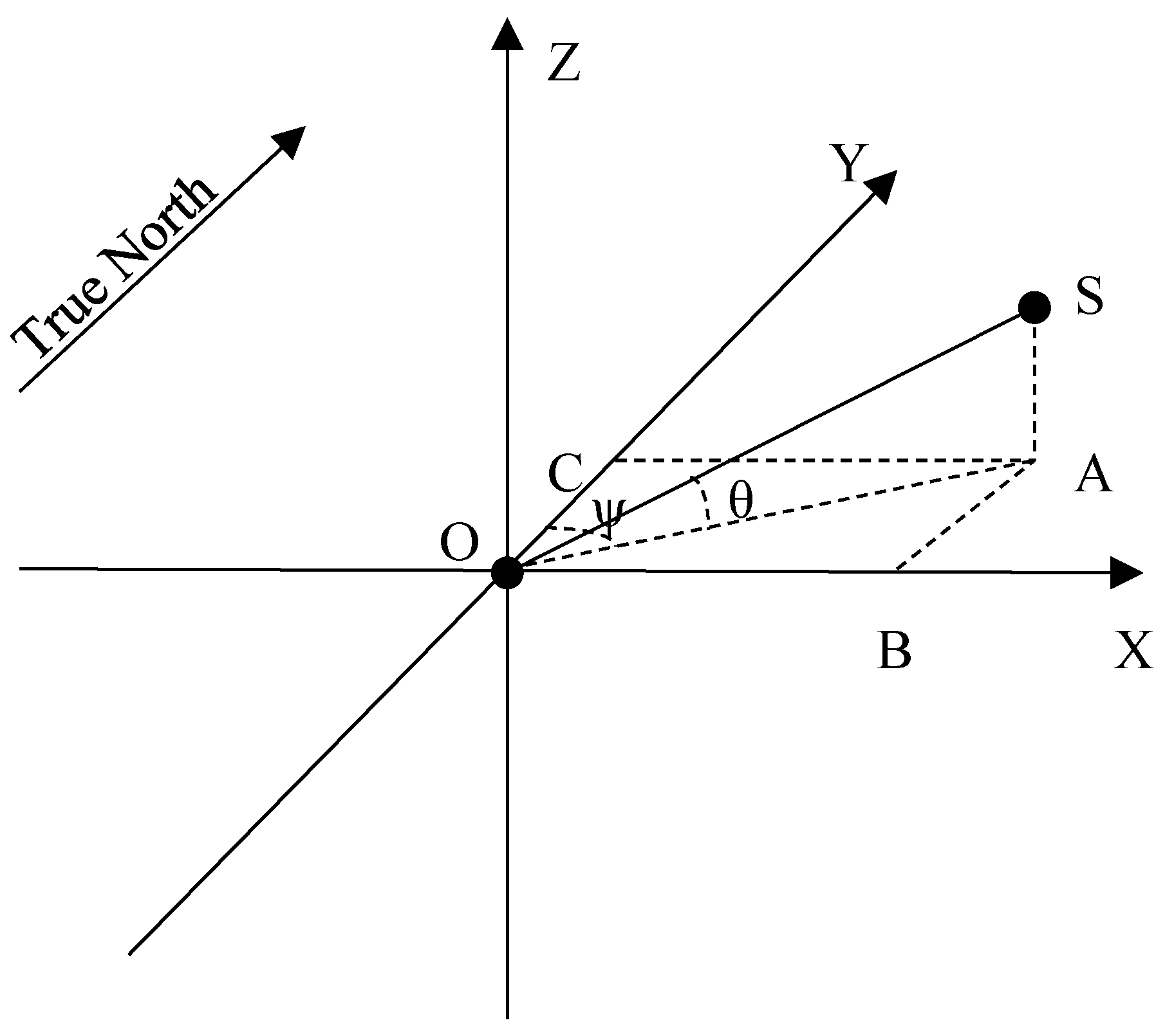
Figure 2 provides the definition of the local Cartesian coordinate system. The point O is the surface point that one sensor pixel observes, and it is regarded as the point of origin. The coordinates for point O are in the WGS84 geocentric system, and they can be transformed into in the geographic coordinate system. The local Cartesian coordinate system is expressed in the Cartesian form, such that the Y-axis lies on the tangent plane in the direction of true north, and the Z-axis is normal to the tangent plane pointing away from the earth (with the X axis completing a right-handed triad, as usual).
The conversion matrix from the WGS84 geocentric system to the local Cartesian coordinate system comprises two simple rotations: (1) a rotation about the Earth’s axis (through angle ) from the Greenwich meridian to the meridian of the local ground; and, (2) a rotation about an axis that is perpendicular to the meridian plane of the local ground (through angle ) from the North Pole to the local ground. The conversion matrix can be expressed as follows:
Taking into consideration Equations (9) and (10), the viewing vector in the local Cartesian coordinate system can be described as follows:
2.2.3. Calculating the Viewing Zenith and Azimuth Angles
Once the viewing vector in the local Cartesian coordinate system is obtained, then the viewing zenith and azimuth angles can be calculated. As shown in Figure 3, the coordinates are the local Cartesian coordinate system, in which the point of origin is O, and S denotes the sensor. Thus, the vector SO is the viewing vector proportional to the vector . Line SA crosses S and is perpendicular to plane XOY at point A. Line AB is perpendicular to plane XOZ and crosses line OX at point B. Line AC is perpendicular to plane YOZ and crosses line OY at point C. Then, is the zenith angle , and is the azimuth angle .
SO is proportional to vector and this equation can be derived as follows:
where m is the scale parameter. Then, the zenith angle and the azimuth angle can be expressed as follows:
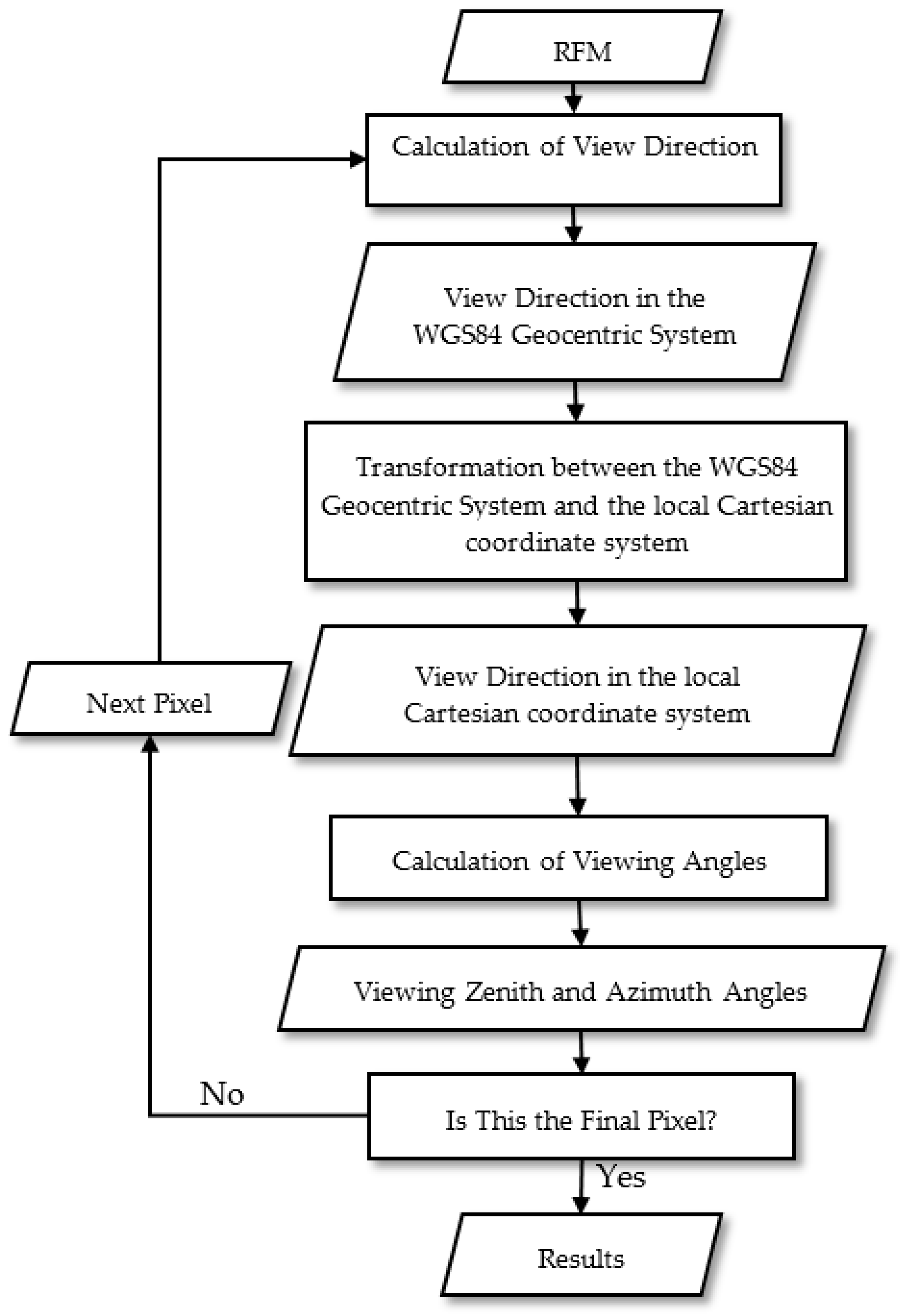
2.3. Workfolow
The process workflow is illustrated in Figure 4, and incorporates steps that can be summarized as follows:
- (1)
- The RFM is obtained, and the view direction in the WGS84 geocentric system is calculated based on the space-vector information of observed light implied by the RFM.
- (2)
- The viewing direction is transformed from the WGS84 geocentric system to the local Cartesian coordinate system.
- (3)
- The viewing zenith and azimuth angles can be calculated in the local Cartesian coordinate system.
- (4)
- If there are pixels that are not calculated, then the first three steps are repeated to solve the next pixel. Finally, all of the the zenith and azimuth angles for all pixels are outputted.
3. Results and Discussion
To verify the correctness and stability of the proposed method, experiments were performed with GF-1’s WFV-1 sensor and ZY3-02’s NAD sensor data. In this section, the two test datasets and the experimental results will be discussed.
3.1. Test Datasets and Evaluation Criterion
The first dataset is from GF-1’s WFV-1 L1 imagery, specifically the RFM file that was taken on 5 October 2013 in Macheng, Hubei Province, China. The image size is 12,000 × 14,400 pixels. The field of view (FOV) for GF-1’s WFV-1 sensor is approximately 16.9°. The elevation of the area varies from 2810 m to 3160 m.
The second dataset is from ZY3-02’s NAD Level-1 imagery, specifically the RFM file taken on 9 March 2017 in Fuzhou, Fujian Province, China. The image size is 24,576 × 24,576 pixels. The FOV for ZY3-02’s NAD sensor is approximately 6°, and the elevation of the area varies from 0 m to 950 m.
In order to verify the correctness and the stability of the proposed method, the RSM parameters were obtained from the original Level-0 products. Then, the angles calculated with the method above were compared with the angles that were calculated using the real parameters from the original Level-0 products. This comparison was used as the evaluating criterion in the verification of the proposed method. This comparison process can be conducted as follows:
- (1)
- Establish the rigorous geometric model based on the corresponding original Level-0 products including interior and exterior parameters.
- (2)
- Calculating the viewing angles of any pixel by the rigorous geometric model established in step 1) using Equation (6) and by the proposed method separately, and then the deviation is calculated.
- (3)
- Statistics deviations of all pixels to calculate the minimum, maximum, and root mean square (RMS).
3.2. Minimum and Maximum Elevation Plane for Calculation
In general, the lowest and highest elevations can be obtained in accordance with the RFM file. However, it is pertinent to establish by experimentation whether this is the best method. In these experiments, the influence of the minimum and maximum elevation can be determined by examining the differences between the angles calculated from the method above and the angles that were calculated from the real parameters of the original Level-0 products.
Table 1 shows the level of precision in GF-1’s WFV-1 viewing angles calculated from the RFM. Item 1 is based on the lowest and highest elevation that was obtained from the RFM file for the sake of comparison under other circumstances. Item 2 shows that the results are very good when there is little distance between the lowest and the highest elevation. Items 3 and 5 reveal that the precision is lower when the maximum elevation increases. Item 4 is included in order to examine the level of precision when the lowest elevation drops. As shown in Table 1, the precision is very high and stable when the elevation is between −10,000 m and +10,000 m. Therefore, the method is not sensitive to the elevations, and shows good stability in this dataset.
In the second dataset, the elevation varies from 0 m to 950 m obtained from corresponding RFM. Thus, different minimum and maximum elevations are set under different circumstances (see Table 2), and the level of precision can be obtained.
Item 1 in Table 2 is based on the lowest and highest elevation that was obtained from the RFM for the sake of comparison with other circumstances. Item 2 shows that the results are considerably precise when there is little distance between the lowest and the highest elevation. Items 3 and 5 reveal that the precision decreases as the maximum elevation increases. Item 4 is included in order to examine the level of precision as the lowest elevation drops. As with the first dataset, Table 2 shows highly precise and stable results for elevations between −10,000 m and +10,000 m. Therefore, the method is not sensitive to the elevations with the stability in this dataset. Moreover, Table 2 also suggests that the elevations are in accordance with the minimum and maximum elevations that were yielded by the RFM, and are the optimal scheme in this dataset.
The above two experiments demonstrate that the method is appropriately insensitive to elevation. The differences are especially small and stable when the elevation is between –10,000 m and +10,000 m, and the results are precise when the distance between the lowest and the highest elevation is small. In general, the minimum and maximum elevation values are set in accordance with the RFM file, because the RFM uses the minimum and maximum elevations for fitting.
3.3. Precision of RFM-Calculated Viewing Angles
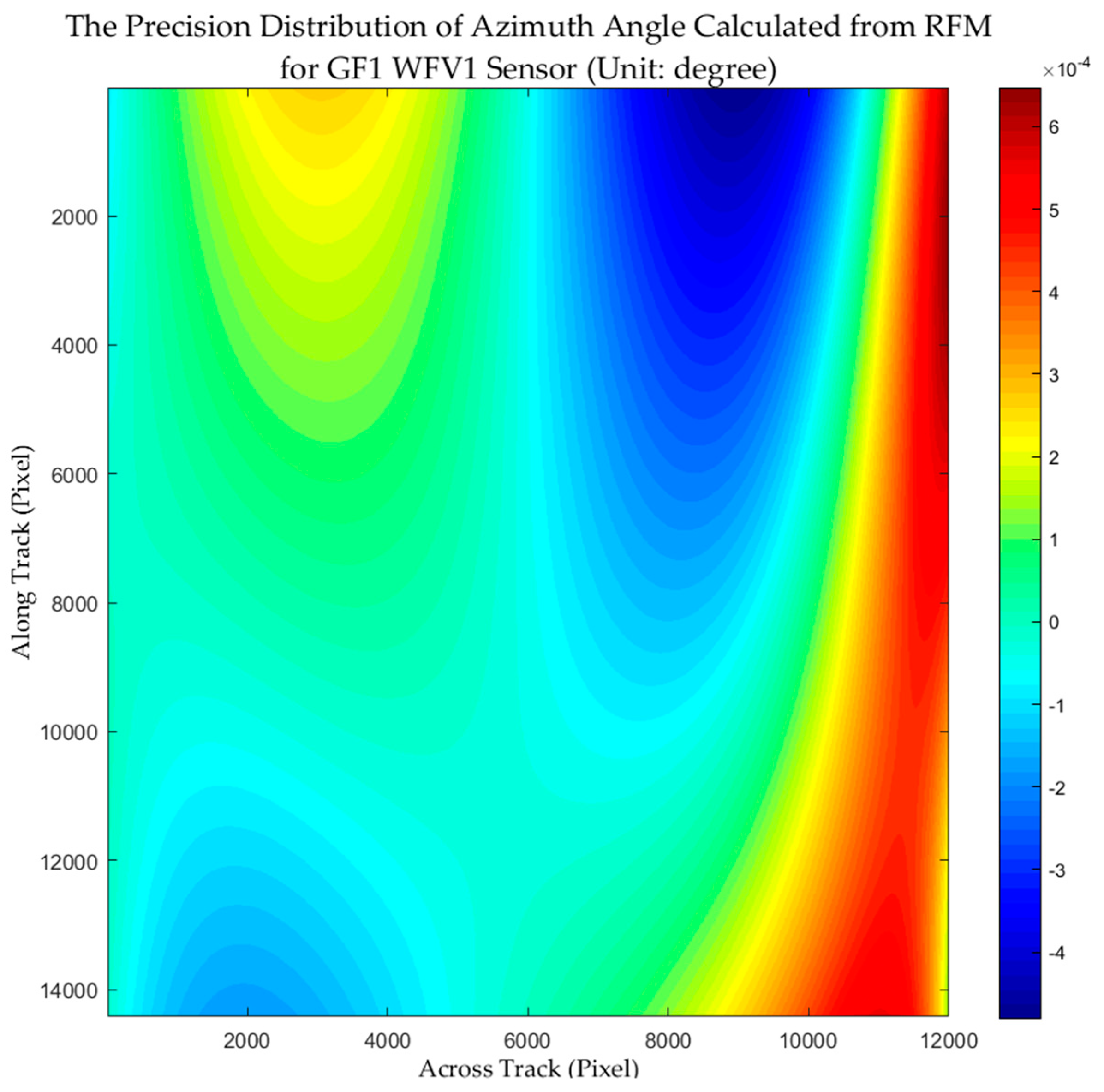
In order to verify the accuracy of the proposed method, the precision can be assessed by examining the differences between the angles that were calculated using the proposed method and the angles calculated using the real parameters from the original Level-0 products. Thus, checkpoints were established on the image plane in 10-pixel intervals. Every checkpoint calculates two groups of viewing angles, after which the two groups of angles can be compared in order to examine the differences between them and thus to verify the accuracy of the proposed method. The precision distribution for the viewing angles from GF-1’s WFV-1 sensor on the image plane is shown in Figure 5.
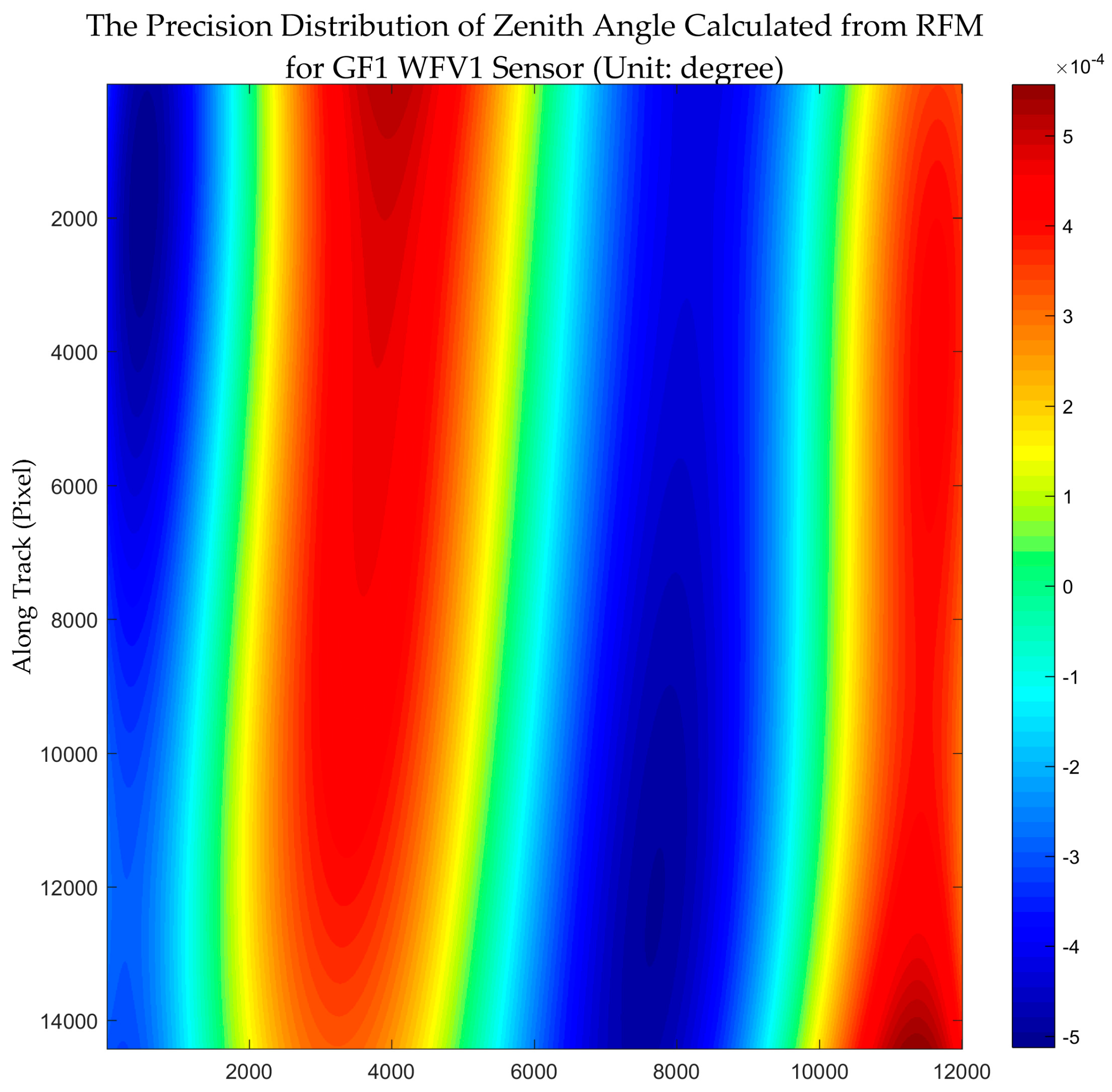
The precision of the viewing angles from GF-1’s WFV-1 sensor is approximately 10–40. However, the precision distribution is relatively irregular. The precision of the azimuth angle, as calculated from the RFM, is high in the middle plane, but drops on going away from the center. In the top-right corner of the plane, there is a sudden change from negative to positive. As shown in Figure 6, the precision of the zenith angle, as calculated from the RFM, is roughly similar along the track, repeating a transformation from negative to positive across the track. Overall, the precision of the viewing angles from GF-1’s WFV-1 sensor meets the requirements in terms of precision and stability.
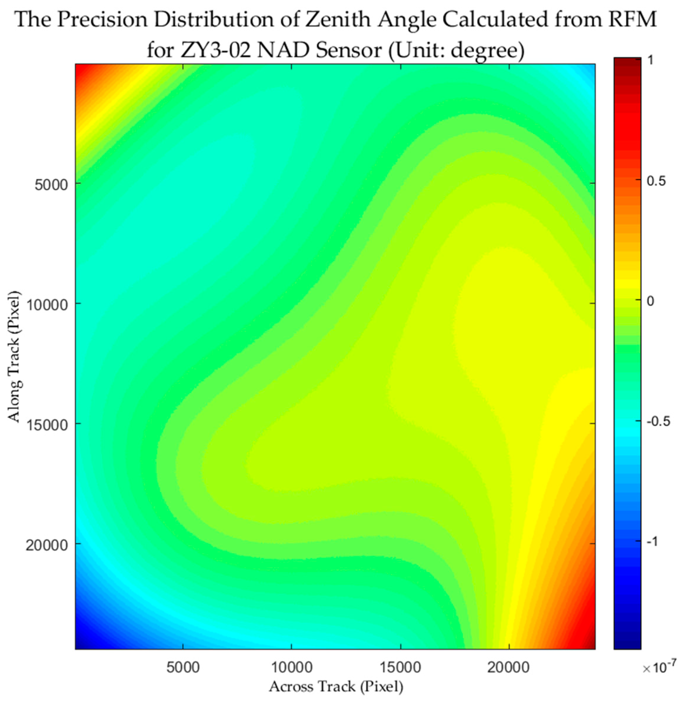
The experiment with ZY3-02’s NAD sensor dataset was performed using the same steps, and the precision distribution for the viewing angles from ZY3-02’s NAD sensor on the image plane is shown in Figure 7 and Figure 8.
The precision of the viewing angles for ZY3-02’s NAD sensor is approximately 10–70. This time, however, the precision distribution is relatively regular. The precision of the azimuth angle calculated from the RFM is roughly similar along the track and across the track in its transformation from negative to positive. The precision of the zenith angle calculated from the RFM is high in the middle plane, and drops in direction away from the center. In the top-left and bottom-right corners, the precision of the zenith angle is positive, whereas in the top-right and bottom-left corners the precision is negative. Overall, the precision of the viewing angles from ZY3-02’s NAD sensor meets the actual requirements both in terms of stability and precision.
Theoretically, the viewing angles calculated from the RFM should be strictly equal to the real parameters from the original Level-0 products. However, because of the residual fitting of the RFM from attitude jitters, time jumps, or higher-order aberrations when the RFM is generated, differences emerge between the angles that are calculated from the RFM and the real parameters of the original Level-0 products. From the described experiments, it is apparent that the precision distribution of angles calculated from GF-1’s WFV-1 sensor RFM is more irregular than the angles that are calculated from ZY3-02’s NAD sensor RFM, and the precision of the angles from ZY3-02’s NAD is three orders of magnitude higher than that of the angles from GF-1’s WFV-1. The FOV of GF-1’s WFV-1 is approximately 16.9°, whereas the FOV of ZY3-02’s NAD is approximately 6°. A wide-field view means higher distortion at the edge of the field, and the residual fitting of the RFM for a wide-field view is relatively larger than the narrow-field view. Thus, the precision distribution of GF-1’s WFV-1 is more irregular and less precise.
In order to examine the statistical properties related to precision, we calculated the RMS in terms of the maximum and minimum precision (Table 3).
The precision of the GF-1’s WFV-1 sensor is similar between the azimuth angle and the zenith angle. The RMS for the azimuth angle is 0.00020°, whereas for the zenith angle, it is 0.00032°. The maximum of the azimuth angle is 0.00065°, while the maximum of the zenith angle is 0.00056°. Thus, the precision is approximately 10–40, and the maximum precision is approximately two or three times that of the RMS. These results confirm that the method as employed for the GF-1’s WFV-1 dataset is accurate and stable.
The precision of the ZY3-02’s NAD sensor is similar between the azimuth and zenith angles. The RMS of the azimuth angle is 0.00000024°, while that of the zenith angle is 0.000000028°. The maximum of the azimuth angle is 0.00000085°, whereas the maximum of the zenith angle is 0.000000145°. Thus, the precision is approximately 10–70 and the maximum precision is several times that of the RMS. Again, these results demonstrate that the method employed for the ZY3-02’s NAD dataset is both accurate and stable.
The accuracy and stability of the method has been successfully verified through the experiments described above, which demonstrated its feasibility for practical applications. The precision is approximately 10−40 for the GF-1’s WFV-1 sensor data, and approximately 10−70 for the ZY3-02’s NAD sensor data.
4. Conclusions
Relying on the commonly used RFM in high-resolution satellite imagery, this study proposed a new method for the determination of viewing angles based on the space-vector information from the observed light implied by the RFM. In deriving the method, we observed that it does not require specific forms of the geometry model. Indeed, every geometric model that can be written as either an implicit or explicit function to describe the geometric relationship between an object point and its image coordinates can use this method to calculate the viewing angles in satellite imagery. Moreover, with the proposed method, the viewing angles for each pixel are calculated independently. That is, the proposed method calculates viewing angles pixel by pixel. Even though geometric transformation is applied to the imagery (e.g., geometric correction or re-projection), it is possible to calculate the viewing angles in pixel-by-pixel fashion, provided that the geometric model is available.
In the proposed method, only the minimum and maximum elevation planes are uncertain, and only they will influence the results. The experiments that were conducted here demonstrate that the method is not sensitive to elevation. The differences are noticeably small and stable when the elevation is between −10,000 m and +10,000 m, and the results are more precise when there is little distance between the lowest and the highest elevation. In general, the optimal elevations are in agreement with the minimum and maximum elevations that are offered by the RFM, because the RFM uses the minimum and maximum elevations for fitting.
Finally, the experiments showed that the precision of the method relative to the real data is approximately 10–40 for the GF-1’s WFV-1 sensor and approximately 10–70 for the ZY3-02’s NAD sensor. The FOV of GF-1’s WFV-1 is approximately 16.9°, whereas the ZY3-02’s NAD is approximately 6°. The wide-field view resulted in high distortion at the edge of the field, and the residual fitting of the RFM for the wide-field view was relatively larger than that for the narrow-field view. Thus, the precision distribution of GF-1’s WFV-1 is more irregular and less precise than that of ZY3-02’s NAD. Overall, the method meets the actual demands in terms of precision and stability for both the GF-1’s WFV-1 sensor and the ZY3-02’s NAD sensor. It is predicted that the method will also meet the requirements of other sensors that are not included in our experiments, and with a comparable level of precision. Despite the promising results that were achieved by comparing with the result acquired from RSM, the proposed method is not yet applied to quantitative remote sensing practically. Thus, the implementation of calculating viewing angles pixel by pixel using RFM for the extraction of surface physical parameters needs further research.
Acknowledgments
This work was supported by, Key research and development program of Ministry of science and technology (2016YFB0500801), National Natural Science Foundation of China (Grant No. 91538106, Grant No. 41501503, 41601490, Grant No. 41501383), China Postdoctoral Science Foundation (Grant No. 2015M582276), Hubei Provincial Natural Science Foundation of China (Grant No. 2015CFB330), Special Fund for High Resolution Images Surveying and Mapping Application System (Grant No. AH1601-10), Quality improvement of domestic satellite data and comprehensive demonstration of geological and mineral resources (Grant No. DD20160067). The authors also thank the anonymous reviews for their constructive comments and suggestions.
Author Contributions
Kai Xu, Guo Zhang and Deren Li conceived and designed the experiments; Kai Xu, Guo Zhang, and Qingjun Zhang performed the experiments; Kai Xu, Guo Zhang and Deren Li analyzed the data; Kai Xu wrote the paper.
Conflicts of Interest
The authors declare no conflict of interest.
References
- Dickinson, R.E. Land processes in climate models. Remote Sens. Environ. 1995, 51, 27–38. [Google Scholar] [CrossRef]
- Mason, P.J.; Zillman, J.W.; Simmons, A.; Lindstrom, E.J.; Harrison, D.E.; Dolman, H.; Bojinski, S.; Fischer, A.; Latham, J.; Rasmussen, J. Implementation Plan for the Global Observing System for Climate in Support of the UNFCCC (2010 Update). Lect. Notes Phys. 2010, 275, 287–306. [Google Scholar]
- Wang, Z.J.; Coburn, C.A.; Ren, X.M.; Teillet, P.M. Effect of surface roughness, wavelength, illumination, and viewing zenith angles on soil surface BRDF using an imaging BRDF approach. Int. J. Remote Sens. 2014, 35, 6894–6913. [Google Scholar] [CrossRef]
- Sims, D.A.; Rahman, A.F.; Vermote, E.F.; Jiang, Z.N. Seasonal and inter-annual variation in view angle effects on MODIS vegetation indices at three forest sites. Remote Sens. Environ. 2011, 115, 3112–3120. [Google Scholar] [CrossRef]
- Van Leeuwen, W.J.; Huete, A.R.; Laing, T.W.; Didan, K. Vegetation change monitoring with spectral indices: The importance of view and sun angle standardized data. In Remote Sensing for Earth Science, Ocean, and Sea Ice Applications; International Society for Optics and Photonics: Bellingham, WA, USA, 1999; p. 10. [Google Scholar]
- Bognár, P. Correction of the effect of Sun-sensor-target geometry in NOAA AVHRR data. Int. J. Remote Sens. 2003, 24, 2153–2166. [Google Scholar] [CrossRef]
- Bucher, T.U. Directional effects (view angle, sun angle, flight direction) in multi-angular high-resolution image data: Examples and conclusions from HRSC-A(X) flight campaigns. Proc. SPIE Int. Soc. Opt. Eng. 2004, 5239, 234–243. [Google Scholar]
- Pocewicz, A.; Vierling, L.A.; Lentile, L.B.; Smith, R. View angle effects on relationships between MISR vegetation indices and leaf area index in a recently burned ponderosa pine forest. Remote Sens. Environ. 2007, 107, 322–333. [Google Scholar] [CrossRef]
- Verrelst, J.; Schaepman, M.E.; Koetz, B.; Kneubühler, M. Angular sensitivity analysis of vegetation indices derived from CHRIS/PROBA data. Remote Sens. Environ. 2008, 112, 2341–2353. [Google Scholar] [CrossRef]
- Niu, Z.; Wang, C.; Wang, W.; Zhang, Q.; Young, S.S. Estimating bidirectional angles in NOAA AVHRR images. Int. J. Remote Sens. 2001, 22, 1609–1615. [Google Scholar] [CrossRef]
- Isaacman, A.T.; Toller, G.N.; Barnes, W.L.; Guenther, B.W.; Xiong, X. MODIS Level 1B calibration and data products. In Proceedings of Optical Science and Technology, SPIE’s 48th Annual Meeting; International Society for Optics and Photonics: Bellingham, WA, USA, 2003; p. 11. [Google Scholar]
- Tao, C.V.; Hu, Y. A Comprehensive study of the rational function model for photogrammetric processing. Photogramm. Eng. Remote Sens. 2001, 67, 1347–1357. [Google Scholar]
- Grodecki, J. IKONOS stereo feature extraction—RPC approach. In Proceedings of the 2001 ASPRS Annual Conference, St. Louis, MO, USA, 23–27 April 2001. [Google Scholar]
- Lutes, J. Accuracy analysis of rational polynomial coefficients for Ikonos imagery. In Proceedings of the 2004 Annual Conference of the American Society for Photogrammetry and Remote Sensing (ASPRS), Denver, CO, USA, 23–28 May 2004. [Google Scholar]
- Dial, G.; Bowen, H.; Gerlach, F.; Grodecki, J.; Oleszczuk, R. IKONOS satellite, imagery, and products. Remote Sens. Environ. 2003, 88, 23–36. [Google Scholar] [CrossRef]
- Hashimoto, T. RPC model for ALOS/PRISM images. In Proceedings of the 2003 IEEE International Geoscience and Remote Sensing Symposium, Toulouse, France, 21–25 July 2003; pp. 1861–1863. [Google Scholar]
- Nagasubramanian, V.; Radhadevi, P.V.; Ramachandran, R.; Krishnan, R. Rational function model for sensor orientation of IRS-P6 LISS-4 imagery. Photogramm. Record 2007, 22, 309–320. [Google Scholar] [CrossRef]
- Pan, H.B.; Zhang, G.; Tang, X.M.; Li, D.R.; Zhu, X.Y.; Zhou, P.; Jiang, Y.H. Basic Products of the ZiYuan-3 Satellite and Accuracy Evaluation. Photogramm. Eng. Remote Sens. 2013, 79, 1131–1145. [Google Scholar] [CrossRef]
- Xu, K.; Jiang, Y.H.; Zhang, G.; Zhang, Q.J.; Wang, X. Geometric Potential Assessment for ZY3-02 Triple Linear Array Imagery. Remote Sens. 2017, 9, 658. [Google Scholar] [CrossRef]
- Zhang, G.; Jiang, Y.H.; Li, D.R.; Huang, W.C.; Pan, H.B.; Tang, X.M.; Zhu, X.Y. In-Orbit Geometric Calibration And Validation Of Zy-3 Linear Array Sensors. Photogramm. Record 2014, 29, 68–88. [Google Scholar] [CrossRef]
- Zhang, G.; Xu, K.; Huang, W.C. Auto-calibration of GF-1 WFV images using flat terrain. ISPRS J. Photogram. Remote Sens. 2017, 134, 59–69. [Google Scholar] [CrossRef]
- Lu, C.L.; Wang, R.; Yin, H. GF-1 Satellite Remote Sensing Characters. Spacecr. Recover. Remote Sens. 2014, 35, 67–73. [Google Scholar]
- Madani, M. Real-time sensor-independent positioning by rationalfunctions. In Proceedings of the ISPRS Workshop on Direct versus Indirect Methods of Sensor Orientation, Barcelona, Spain, 25–26 November 1999; pp. 64–75. [Google Scholar]
Figure 1.
Principles for calculating the viewing direction.
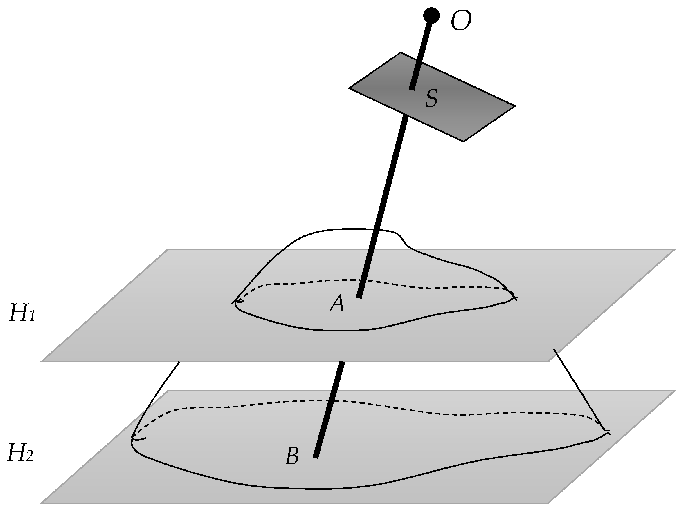
Figure 2.
Definition of the local Cartesian coordinate system.
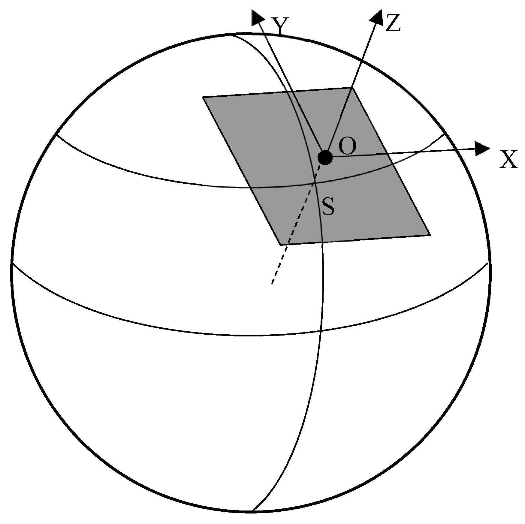
Figure 3.
Calculating the viewing zenith and azimuth angles.

Figure 4.
Calculation process for the Rigorous Sensor Model recovery.

Figure 5.
Precision distribution of the azimuth angle calculated from the Rational Function Model (RFM) for Gaofen-1 (GF-1) Wide-Field-View-1 (WFV-1) sensor (unit: degrees).
Figure 5.
Precision distribution of the azimuth angle calculated from the Rational Function Model (RFM) for Gaofen-1 (GF-1) Wide-Field-View-1 (WFV-1) sensor (unit: degrees).

Figure 6.
Precision distribution for the zenith angle calculated from the Rational Function Model (RFM) for Gaofen-1 (GF-1) Wide-Field-View-1 (WFV-1) sensor (unit: degrees).
Figure 6.
Precision distribution for the zenith angle calculated from the Rational Function Model (RFM) for Gaofen-1 (GF-1) Wide-Field-View-1 (WFV-1) sensor (unit: degrees).

Figure 7.
Precision distribution for the azimuth angle calculated from the Rational Function Model (RFM) for ZY3-02 panchromatic nadir (NAD) sensor (unit: degrees).
Figure 7.
Precision distribution for the azimuth angle calculated from the Rational Function Model (RFM) for ZY3-02 panchromatic nadir (NAD) sensor (unit: degrees).
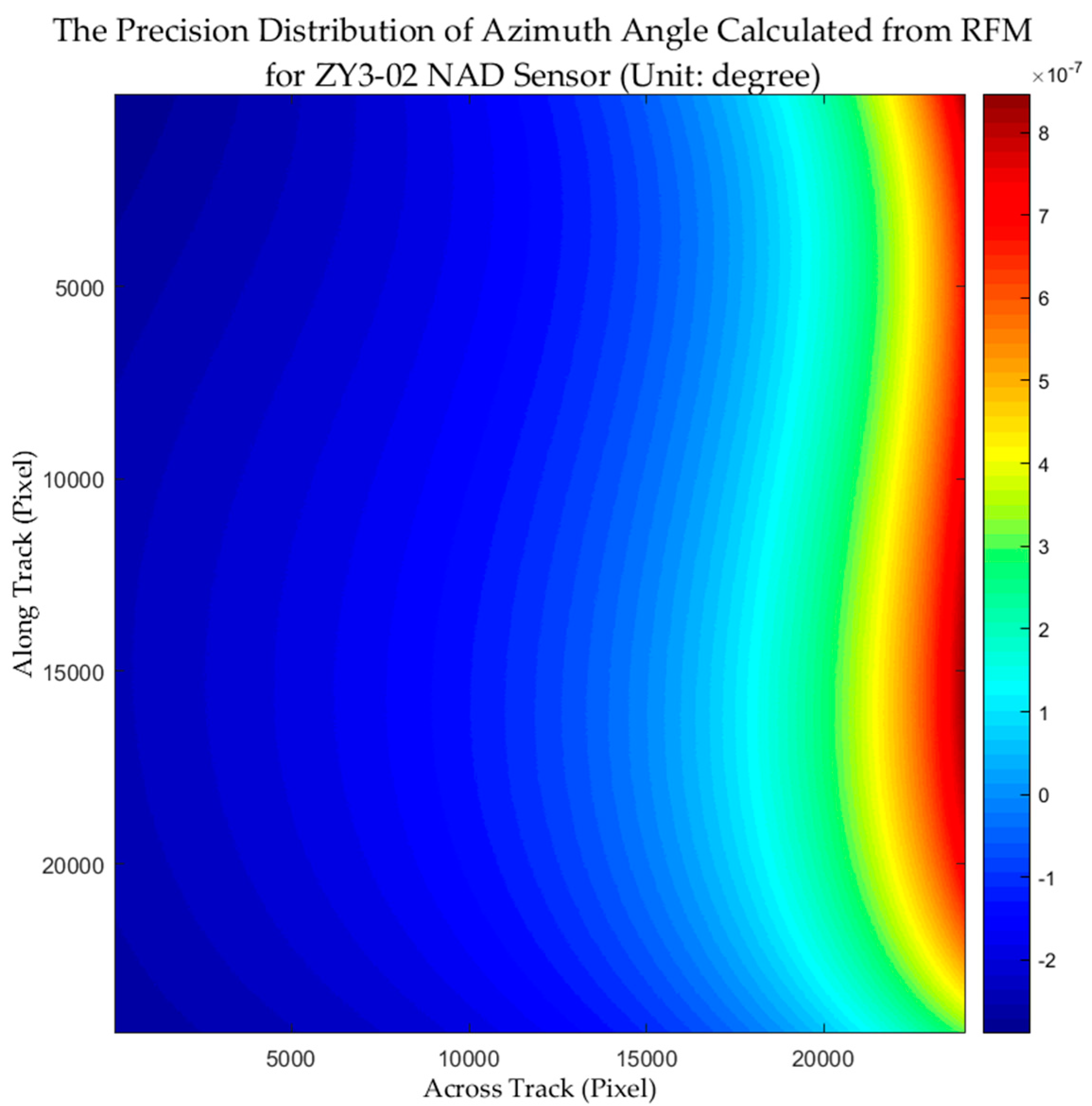
Figure 8.
Precision distribution for the zenith angle calculated from the Rational Function Model (RFM) for ZY3-02 panchromatic nadir (NAD) sensor (unit: degrees).
Figure 8.
Precision distribution for the zenith angle calculated from the Rational Function Model (RFM) for ZY3-02 panchromatic nadir (NAD) sensor (unit: degrees).


Table 1.
Precision of Gaofen-1 (GF-1) Wide Field-of-View-1 (WFV-1) viewing angles calculated from the Rational Function Model (RFM) at planes of different elevations.
Table 1.
Precision of Gaofen-1 (GF-1) Wide Field-of-View-1 (WFV-1) viewing angles calculated from the Rational Function Model (RFM) at planes of different elevations.
| Items | 1 | 2 | 3 | 4 | 5 | |
|---|---|---|---|---|---|---|
| Elevation (m) | Min. Elevation | 2810 | 500 | 0 | −10,000 | 0 |
| Max. Elevation | 3160 | 501 | 10,000 | 10,000 | 100,000 | |
| Azimuth Angle Precision (°) | RMS | 0.00020 | 0.00019 | 0.00027 | 0.00019 | 0.0034 |
| Max. | 0.00065 | 0.00065 | 0.00088 | 0.00056 | 0.0147 | |
| Min. | 0.00000 | 0.00000 | 0.00000 | 0.00000 | 0.0000 | |
| Zenith Angle Precision (°) | RMS | 0.00032 | 0.00032 | 0.00031 | 0.00032 | 0.0089 |
| Max. | 0.00056 | 0.00057 | 0.00070 | 0.00055 | 0.0183 | |
| Min. | 0.00000 | 0.00000 | 0.00000 | 0.00000 | 0.0000 | |
Table 2.
Precision of ZY3-02 panchromatic nadir (NAD) viewing angles calculated from the Rational Function Model (RFM) at planes of different elevations.
Table 2.
Precision of ZY3-02 panchromatic nadir (NAD) viewing angles calculated from the Rational Function Model (RFM) at planes of different elevations.
| Items | 1 | 2 | 3 | 4 | 5 | |
|---|---|---|---|---|---|---|
| Elevation (m) | Min. Elevation | 0 | 500 | 0 | −10,000 | 0 |
| Max. Elevation | 950 | 501 | 10,000 | 10,000 | 100,000 | |
| Azimuth Angle Precision (°) | RMS | 2.3 × 10⁻⁷ | 6.3 × 10⁻⁷ | 5.0 × 10⁻⁶ | 6.8 × 10⁻⁷ | 0.0034 |
| Max. | 8.0 × 10⁻⁷ | 2.8 × 10⁻⁵ | 1.2 × 10⁻⁵ | 2.2 × 10⁻⁶ | 0.0147 | |
| Min. | 0.0000 | 0.0000 | 2.3 × 10⁻⁶ | 0.0000 | 0.0000 | |
| Zenith Angle Precision (°) | RMS | 2.8 × 10⁻⁸ | 8.8 × 10⁻⁸ | 6.5 × 10⁻⁸ | 5.4 × 10⁻⁸ | 0.0089 |
| Max. | 1.5 × 10⁻⁷ | 3.4 × 10⁻⁶ | 3.8 × 10⁻⁷ | 2.5 × 10⁻⁷ | 0.0183 | |
| Min. | 0.0000 | 0.0000 | 0.0000 | 0.0000 | 0.0000 | |
Table 3.
Precision of the viewing angles using the proposed method.
| Items | GF-1’s WFV1 Sensor | ZY3-02’s NAD Sensor | |
|---|---|---|---|
| Azimuth Angle Precision (°) | RMS | 0.00020 | 0.00000024 |
| Max. | 0.00065 | 0.00000085 | |
| Min. | 0.00000 | 0.00000000 | |
| Zenith Angle Precision (°) | RMS | 0.00032 | 0.000000028 |
| Max. | 0.00056 | 0.000000145 | |
| Min. | 0.00000 | 0.000000000 | |
© 2018 by the authors. Licensee MDPI, Basel, Switzerland. This article is an open access article distributed under the terms and conditions of the Creative Commons Attribution (CC BY) license (http://creativecommons.org/licenses/by/4.0/).
Share and Cite
MDPI and ACS Style
Xu, K.; Zhang, G.; Zhang, Q.; Li, D. Calculating Viewing Angles Pixel by Pixel in Optical Remote Sensing Satellite Imagery Using the Rational Function Model. Remote Sens. 2018, 10, 478. https://doi.org/10.3390/rs10030478
AMA Style
Xu K, Zhang G, Zhang Q, Li D. Calculating Viewing Angles Pixel by Pixel in Optical Remote Sensing Satellite Imagery Using the Rational Function Model. Remote Sensing. 2018; 10(3):478. https://doi.org/10.3390/rs10030478
Chicago/Turabian StyleXu, Kai, Guo Zhang, Qingjun Zhang, and Deren Li. 2018. "Calculating Viewing Angles Pixel by Pixel in Optical Remote Sensing Satellite Imagery Using the Rational Function Model" Remote Sensing 10, no. 3: 478. https://doi.org/10.3390/rs10030478
Note that from the first issue of 2016, this journal uses article numbers instead of page numbers. See further details here.