Article

Improving SMOS Sea Surface Salinity in the Western Mediterranean Sea through Multivariate and Multifractal Analysis

by
Estrella Olmedo
1,*,
Isabelle Taupier-Letage
2,
Antonio Turiel
1 and
Aida Alvera-Azcárate
3
1
Department of Physical Oceanography, Institute of Marine Sciences, CSIC, Barcelona Expert Center, Pg. Marítim 37-49, Barcelona E-08003, Spain
2
Aix Marseille Université, CNRS/INSU, Université de Toulon, IRD, Mediterranean Institute of Oceanography (MIO), F-83507 La Seyne, Marseille, France
3
Département d’astrophys., géophysique et océanographie (AGO), GeoHydrodynamics and Environment Research (GHER), Université de Liège, Allée du 6 Août, 17 Sart Tilman, Liège 4000, Belgium
*
Author to whom correspondence should be addressed.
Remote Sens. 2018, 10(3), 485; https://doi.org/10.3390/rs10030485
Submission received: 23 January 2018 / Revised: 5 March 2018 / Accepted: 17 March 2018 / Published: 20 March 2018
(This article belongs to the Special Issue Sea Surface Salinity Remote Sensing)

Abstract

:
A new methodology using a combination of debiased non-Bayesian retrieval, DINEOF (Data Interpolating Empirical Orthogonal Functions) and multifractal fusion has been used to obtain Soil Moisture and Ocean Salinity (SMOS) Sea Surface Salinity (SSS) fields over the North Atlantic Ocean and the Mediterranean Sea. The debiased non-Bayesian retrieval mitigates the systematic errors produced by the contamination of the land over the sea. In addition, this retrieval improves the coverage by means of multiyear statistical filtering criteria. This methodology allows obtaining SMOS SSS fields in the Mediterranean Sea. However, the resulting SSS suffers from a seasonal (and other time-dependent) bias. This time-dependent bias has been characterized by means of specific Empirical Orthogonal Functions (EOFs). Finally, high resolution Sea Surface Temperature (OSTIA SST) maps have been used for improving the spatial and temporal resolution of the SMOS SSS maps. The presented methodology practically reduces the error of the SMOS SSS in the Mediterranean Sea by half. As a result, the SSS dynamics described by the new SMOS maps in the Algerian Basin and the Balearic Front agrees with the one described by in situ SSS, and the mesoscale structures described by SMOS in the Alboran Sea and in the Gulf of Lion coincide with the ones described by the high resolution remotely-sensed SST images (AVHRR).

Graphical Abstract

1. Introduction

The Mediterranean Sea is a hot spot for climate change [1]. The water balance in the basin is characterized by an excess of evaporation over precipitation and river runoff, which is compensated by the entrance of fresher water from the Atlantic. This Atlantic water (AW), which spreads through the Mediterranean Sea, determines the surface circulation [2]. In the Algerian Basin, AW forms an unstable current that generates fresh-core coastal eddies that propagate downstream [3]. The eddy activity in the region enhances the mixing of the recently entered fresher AW with the saltier resident ones, strongly affecting the spatial distribution of salinity and, therefore, playing a major role in the surface circulation of the Mediterranean Sea ([4,5] and references therein).
Additionally, during winter, in the Northwestern Mediterranean, deep water convection occurs under the influence of dry and cold northerly winds. The result is the Western Mediterranean Deep Water, which contributes to the Mediterranean thermohaline circulation. The budget of salt involved in the Deep Water Formation (DWF) remains an open question (e.g., [6,7]), which is addressed by the HYMEX (HYdrological cycle in the Mediterranean EXperiment [8]) program [9].
Reliable estimates of budgets are indeed critically needed to improve the Mediterranean climate evolution simulations [10,11,12]. Finally, DWF also impacts the ecosystems: the associated winter vertical mixing is responsible for the nutrients enrichment of the surface layer, and therefore contributes to the following spring bloom ([13,14] and references therein).
In such a context, data from Soil Moisture and Ocean Salinity (SMOS) European Space Agency (ESA)’s mission [15,16,17] spanning more than eight years can help to gain a better understanding of the Sea Surface Salinity (SSS) dynamics in the Mediterranean Sea. Unfortunately, this critical area is strongly affected by Radio Frequency Interference (RFI) and systematic biases due to the coast contamination (also called Land-Sea Contamination, (LSC)). Both effects make it very difficult to retrieve SMOS SSS in these areas.
Recently, several studies have been presented showing that retrieving SMOS SSS in the Mediterranean is actually feasible. The first one [18] considers the domain North Atlantic Ocean and the Mediterranean Sea. They start from the official Level 2 Ocean Salinity (L2OS) product (version 550), and, by using DINEOF (Data Interpolating Empirical Orthogonal Functions), the authors reconstruct missing data using a truncated EOF basis. The methodology allows removing part of the biases (for example, the ones associated with the edge of the swath). However, the biases present near land masses (LSC), large scale biases and latitudinal biases are not corrected because they are persistent and retained in dominant EOFs.
In the second one [19], the probability of detecting and following eddies in the Algerian Basin from the SMOS SSS is computed. They also use the SMOS SSS to reconstruct currents in the basin. In this case, the SMOS SSS are retrieved from the Level 1 Brightness Temperature (TB) product (v620) following the methodology proposed in [20], which aims to mitigate the spatial systematic biases (such as the LSC). Furthermore, this methodology applies statistical filtering criteria, which allow for a better removal of those TB degraded by RFI. After that, they improve the spatial and temporal resolution of the products by using the multifractal vectorial fusion algorithm proposed in [21]. Despite the fact that the resulting SMOS SSS maps in the Mediterranean display coherent spatial structures (in comparison with other remotely sensed variables such as the sea surface temperature or height), the authors pointed out that some biases still remain in the Mediterranean when they compare with Argo floats.
The purpose of this work is to improve the quality of the SMOS SSS in the Mediterranean Sea by: (1) better retrieval and filtering of SMOS SSS [20]; (2) deletion of time-dependent residual biases by means of DINEOF [18], and (3) improvement of the spatial and temporal resolutions by use of multifractal fusion [21]. The structure of the work is the following: in Section 2, the different data sets used in our study are described. A brief description of the methodologies is presented in Section 3. The results are shown in Section 4. Finally, Section 5 includes the main findings and lists the prominent conclusions of our work.

2. Data Sets

2.1. Sea Surface Salinity SMOS Data

Three different SMOS data sets have been used in this study:
  • Level 1 B product: the input data for the computation of the product in this work is the Level 1 Brightness Temperature product (L1B v620). This product is the output of the image reconstruction of the SMOS measurements and consists of the Fourier components of brightness temperatures in the antenna polarization reference frame. The latency of the products is 6–8 h. The L1B TB product is distributed by the ESA and it is freely available in [22].
  • Objectively analyzed SMOS SSS maps provided by the Barcelona Expert Center: the global advanced debiased non-Bayesian L3 9-day SSS maps at 0.25 × 0.25 available at [23] have been used for assessing the improvements of our proposed methodology at Level 3.
  • Level 4 SMOS SSS maps provided by the Barcelona Expert Center: The global L4 advanced SSS maps at 0.05 × 0.05 available at [23] have been used also for assessing the proposed methodology at Level 4, after applying the multifractal fusion with the OSTIA SST maps.

2.2. Sea Surface Salinity In Situ Data

Three different sources of in situ SSS data have been used in this study:
  • Argo SSS: SSS data from Argo floats have been used in Section 3.2 for the characterization of the bias of the binned SMOS SSS products. After that, Argo data have been also compared with the resulting SMOS products in Section 4.1. The collocation of SMOS and Argo SSS has been performed as follows: we compare the uppermost SSS measurement provided by the Argo profile at the instant t 0 with the SMOS SSS field given by the 9-day map ( t 0 ± 4 days). The Argo floats present errors on the conductivity records when measurements are done shallower than 0.5 m due to air bubbles. Therefore, those records are not considered for the analysis. Additionally, Argo SSS deeper than 10 m have not been considered in our study.
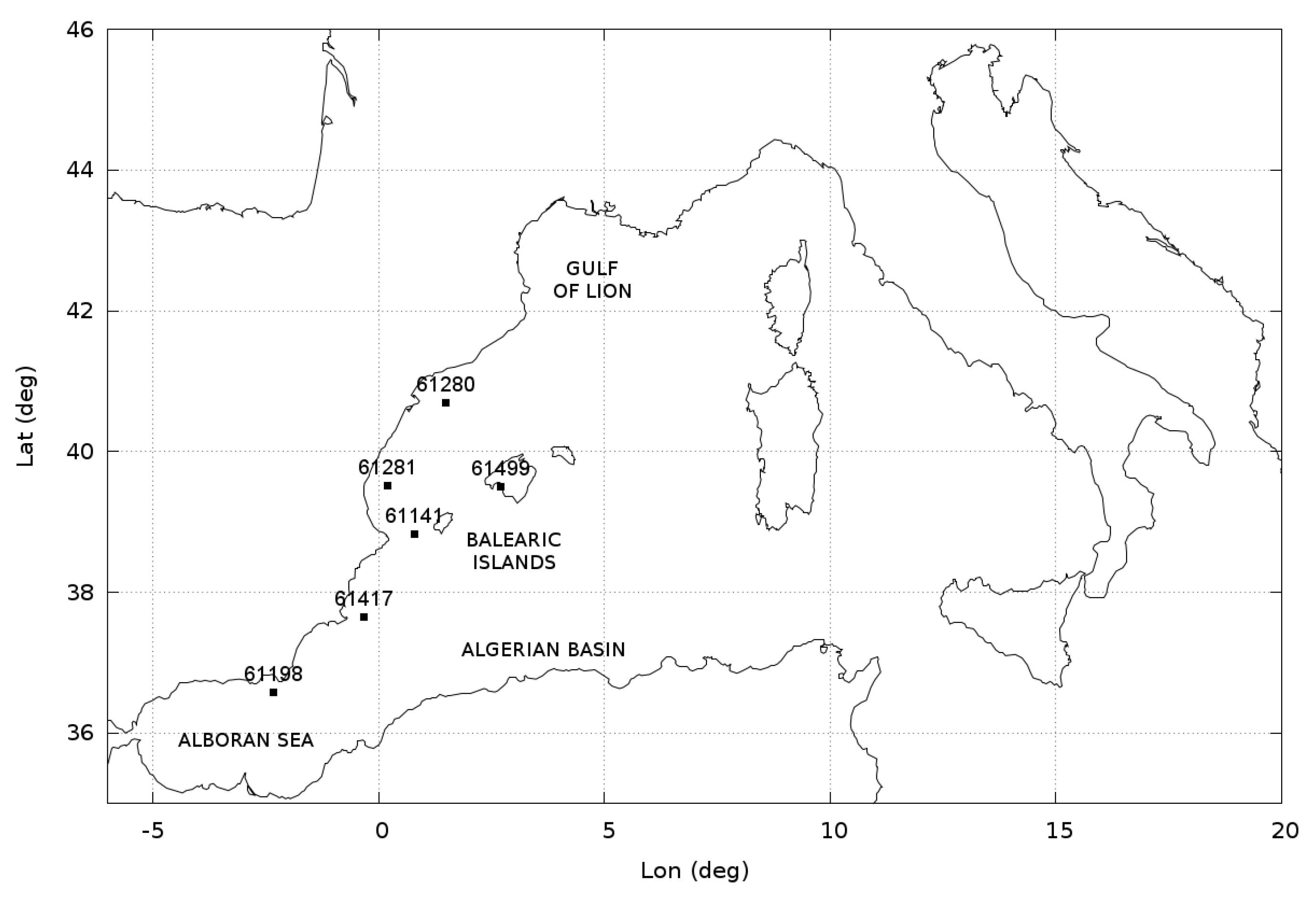
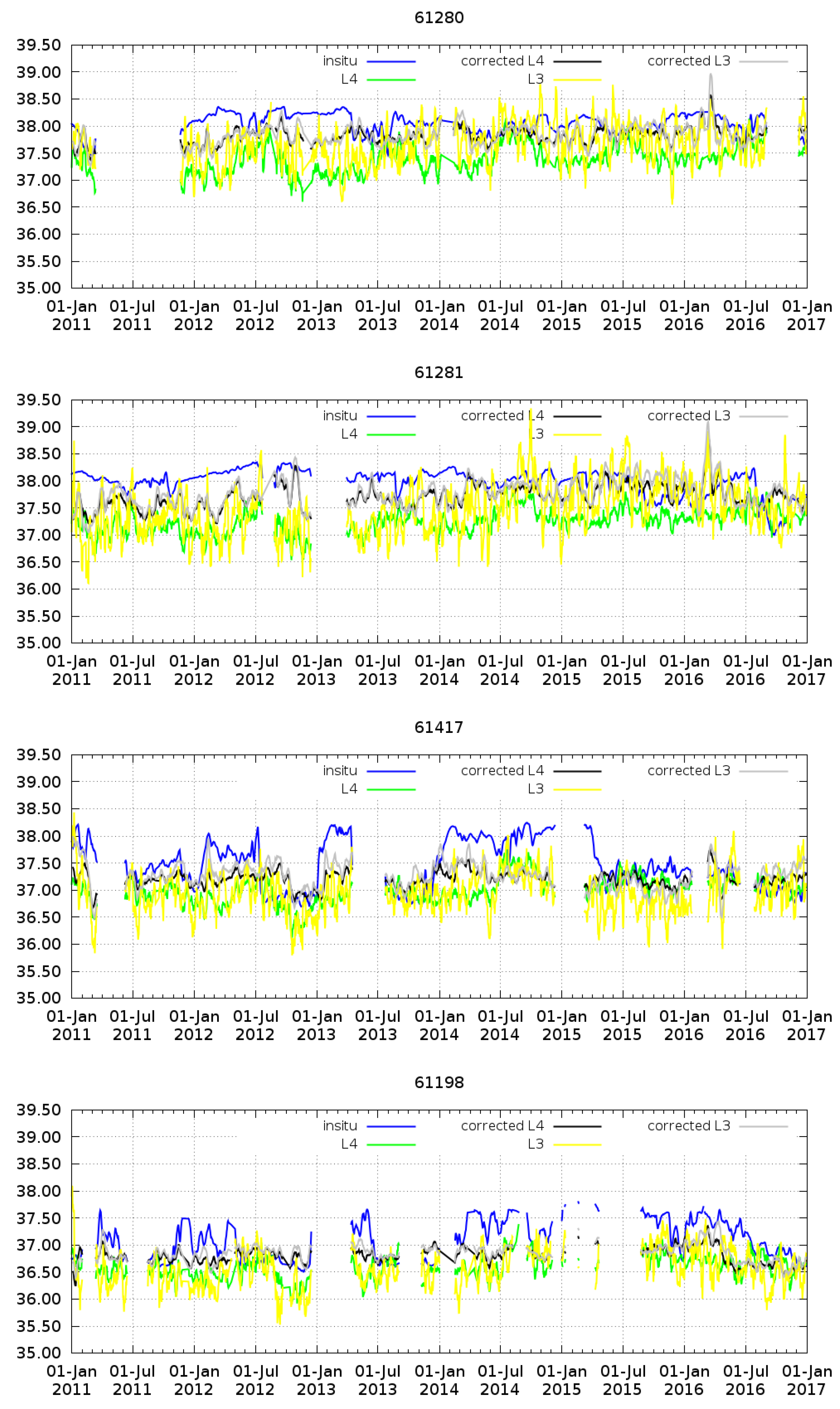
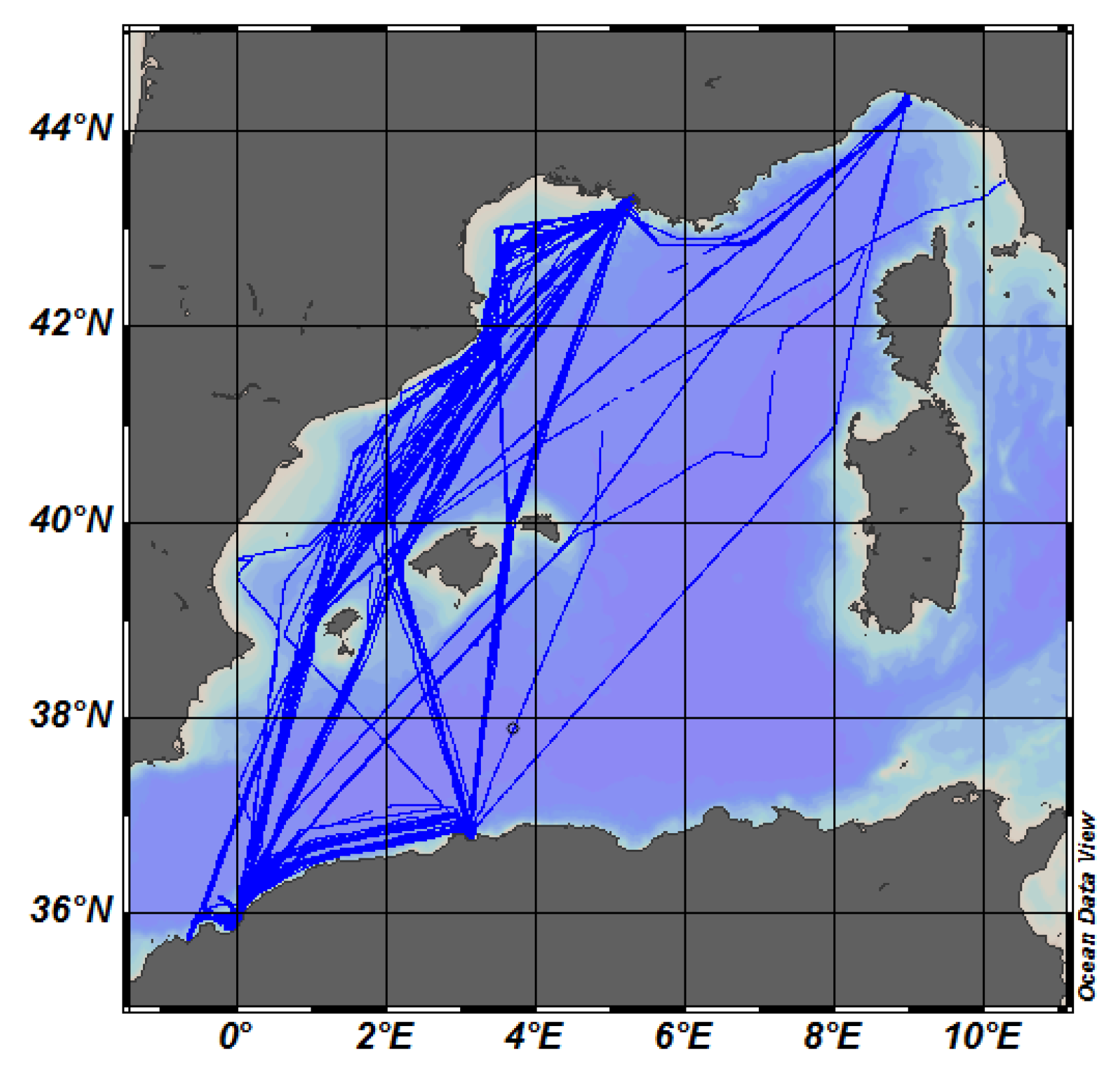
  • SSS time series from six moorings located in the Western Mediterranean have been considered as part of the independent validation process described in Section 4.2 (see their location in Figure 1):
    -
    Four moorings are operated by Puertos del Estado ([24]): the moorings number 61,198, 61,417, 61,281 and 61,280.
    -
    Two moorings are operated by SOCIB (Sistema de Observacion y prediccion Costero de las Islas Baleares): the moorings number 61,141 and 61,499. Data before 2016 have been collected from [25,26]. Data of 2016 have been collected directly from SOCIB website:
    Data in the Ibiza chanel is provided at [27]
    Data in the Palma Bahia is providad at [28]
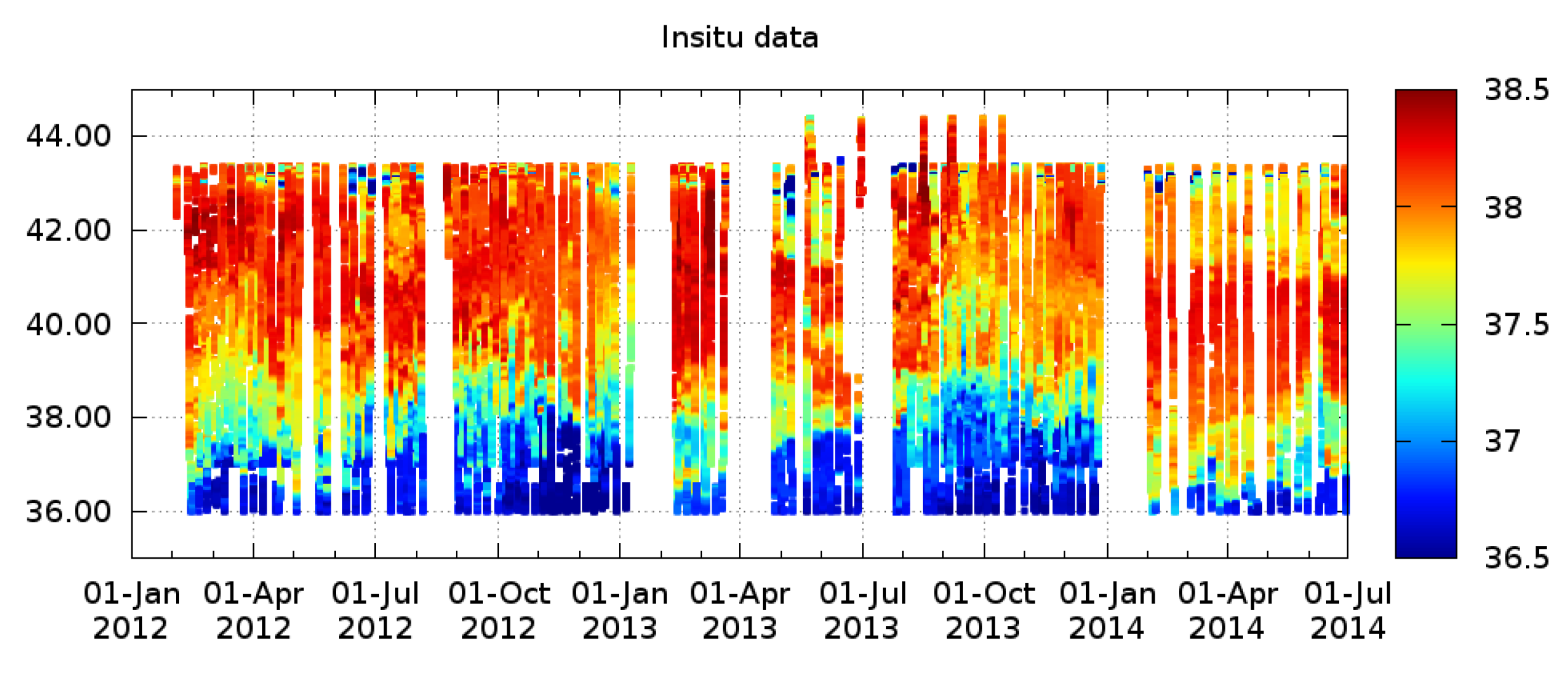
    The collocation between mooring and SMOS SSS has been computed as follows: we have only considered data flagged as “good-quality”. In addition, salinity values out of the range [36:39] PSU (Practical Salinity Units) have been removed from the comparison. A sliding averaging window of nine days has been applied to the mooring data in order to compare both data (satellite and mooring) in a more similar temporal scale. Therefore, the mooring acquisition at time t 0 , which has been filtered with a centered 9-day window, has been compared with the SMOS SSS maps computed from the same 9-day period.
  • Data from the TRANSMED system thermosalinometer, ([29]) on board the MV Marfret Niolon [30] have been used in this study as independent source of data for validation in Section 4.3. Sea Surface Temperature (TRANSMED SST) and Sea Surface Salinity (TRANSMED SSS) are recorded underway at ∼3 m deep, during weekly trips between Marseilles, France, and Algeria. The data has been post-processed following water samples results and yearly recalibration of the thermosalinometers. In this case, the collocation strategy between satellite and in situ data is the same as the one used for the Argo comparison: the TRANSMED SSS acquired at time t 0 has been compared with the SMOS SSS 9-day map with t 0 the mid-day of the 9-day period. Each TRANSMED SSS measurement has been compared with the SMOS SSS corresponding to the cell 0.25 × 0.25 (or 0.05 × 0.05 in the case of L4) corresponding to the TRANSMED SSS location.

2.3. Sea Surface Temperature Data

Two different sources of Sea Surface Temperature have been used:
  • The 0.05 × 0.05 daily Operational Sea Surface Temperature and Sea Ice Analysis (OSTIA) product (see [31]) has been used for the generation of the SMOS SSS L4 products (hereafter OSTIA SST). The OSTIA system is part of the Group for High Resolution Sea Surface Temperature (GHRSST). Access to OSTIA data is available at [25]. The OSTIA output is a daily global coverage combined SST and sea-ice concentration product on a 1/20deg. grid, based on measurements from several satellite and in situ SST data sets. OSTIA uses SST data in the common format developed by GHRSST and makes use of the uncertainty estimates and auxiliary fields as part of the quality control and analysis procedure. Satellite derived sea ice products from the EUMETSAT Ocean and Sea Ice Satellite application Facility (OSI-SAF) provide sea-ice concentration and edge data to the analysis system. After quality control of the SST observations, a bias correction is performed using ATSR-2/AATSR data as a key component. To provide the final SST analysis, a multi-scale optimal interpolation (OI) is performed using the previous analysis as the basis for a first guess field.
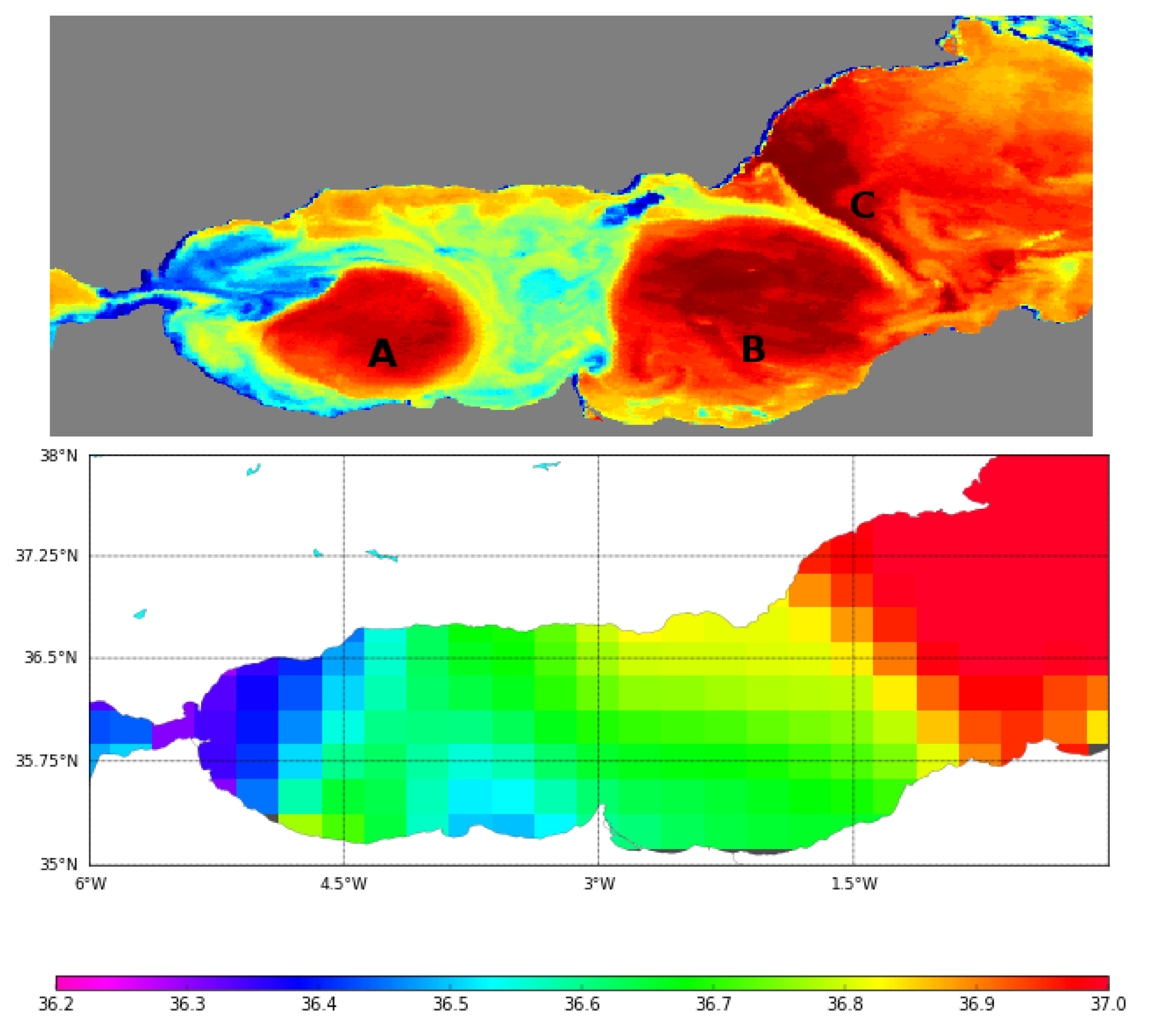
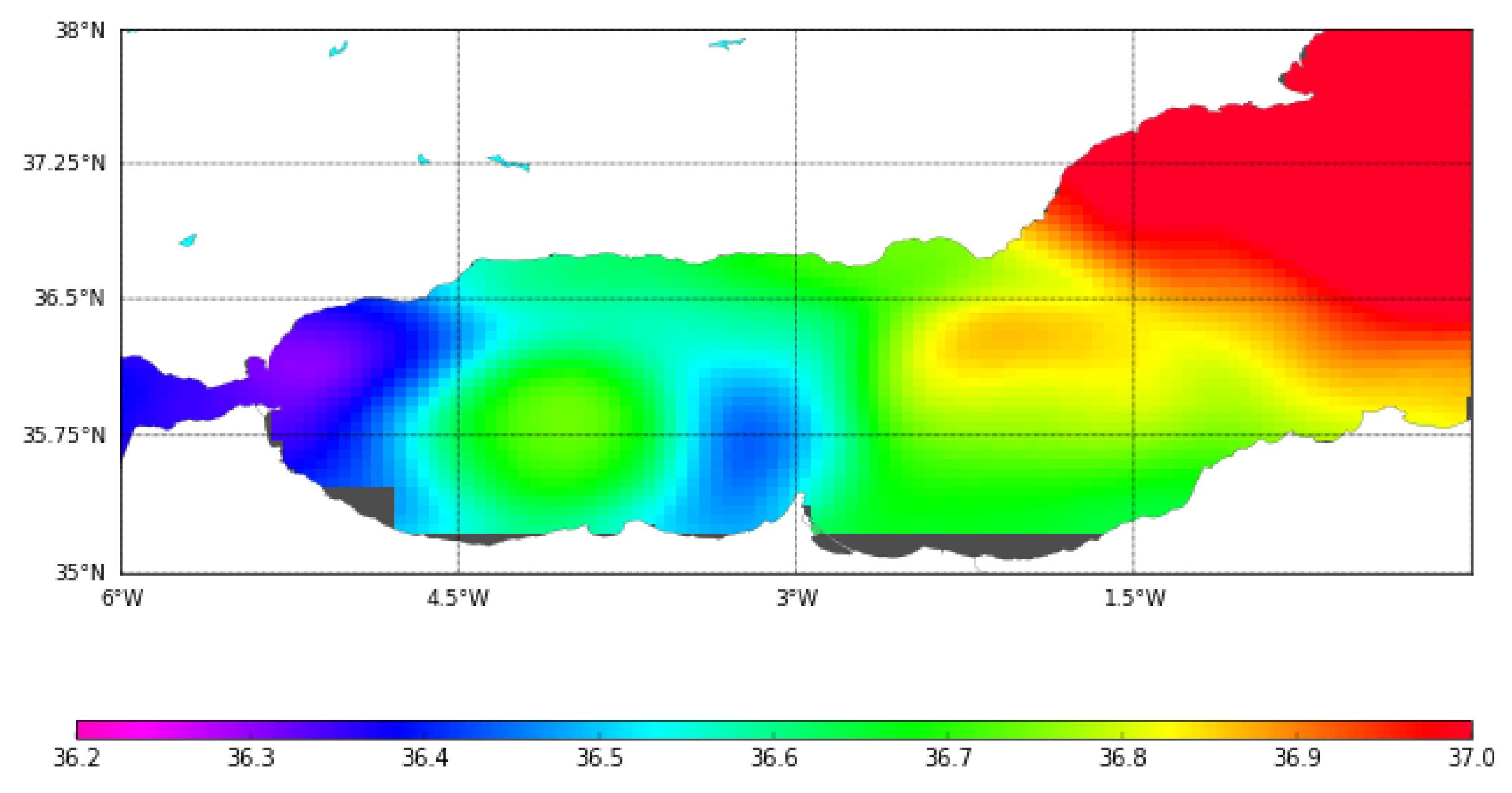
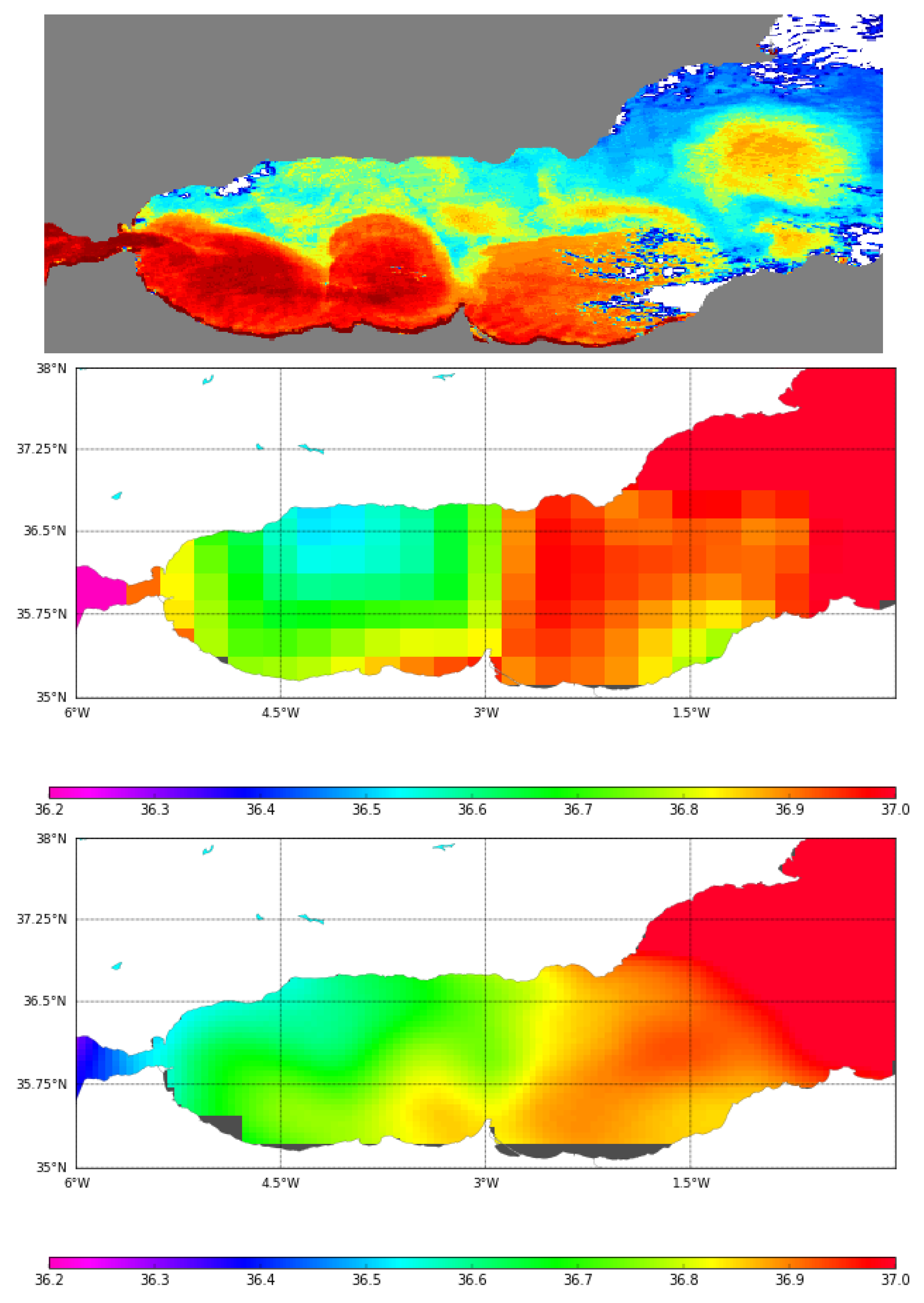
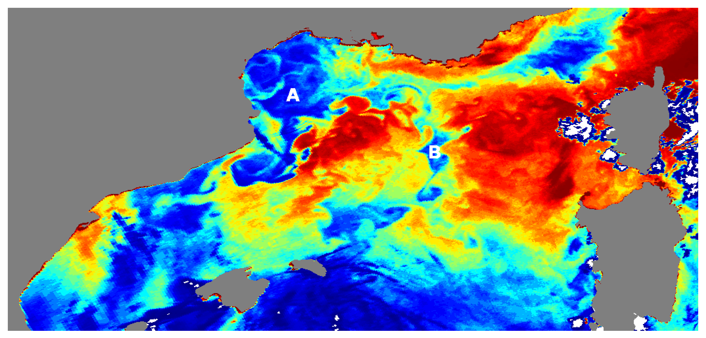
  • Images of Brightness Temperature (Advances Very High Resolution Radiometer (AVHRR) channel 4) from satellites National Atmospheric and Oceanic Administration (NOAA) / AVHRR sensors at 1 × 1 km have been used in Section 4.4 as reference data set in a qualitative assessment of the resulting spatial structures of the SMOS SSS products. Brightness temperature images (hereafter AVHRR images) are produced by the SATMOS (CNRS INSU/MeteoFrance) at the CMS Lannion from NOAA/AVHRR images, and processed at MIO (Available online: [32] (accessed on 19 March 2018)), (see [33]). Brightness Temperatures are relative temperatures, and the color scale is stretched to enhance the structures. These images do not include any compositing, and hence provide the best visualisation of the structures. As a result, the color scale is not relevant and it will not be included.

3. Methods

This section summarizes the steps realized to obtain fields of SSS over the North Atlantic Ocean and the Mediterranean Sea using a combination of a debiased non-Bayesian retrieval, DINEOF and multifractal fusion. The starting point of our study is the Level 1 Brightness Temperatures (L1B v620) product provided by the ESA.

3.1. Debiased Non-Bayesian Retrieval of SSS

The retrieval of SSS from SMOS TB is quite challenging in areas affected by the presence of systematic biases such as LSC or RFI. The standard retrieval scheme is based on a Bayesian approach, which is based in a Maximum Likelihood Estimator of the geophysical parameters obtained by assuming that the errors on TBs are independent and Gaussian-distributed, a hypothesis that poorly adapts to real conditions in the Mediterranean Sea and precludes obtaining quality retrievals in that region. A different approach is provided by the non-Bayesian approach [20,34], in which no hypothesis about the distribution or the correlation of the errors is made. Thus, each single TB measurement is used to derive a noisy estimate of SSS. In [20], these retrievals are later classified according to their geographical (latitude/longitude coordinates) and orbital characteristics (position in the antenna, overpass direction) to correct common biases. This classification allows to define a SMOS-based climatology for each acquisition condition which allows removing systematic biases and also defining proper filtering criteria (based on the statistical properties of each class of salinities), which allow discarding those measurements with a deviation from the reference value that cannot be explained by the radiometric variability. Therefore, SMOS-based anomalies are computed by subtracting their corresponding SMOS-based climatology to each retrieval. The debiased SSS field is obtained when an annual SSS reference (the annual World Ocean Atlas 2013 SSS at 0.25 × 0.25 ([35]) is considered) is added to the SMOS-based anomalies. For each satellite overpass, at every point (i.e., each dwell line), the corrected measurements are thus averaged together to obtain a non-Bayesian L2 SSS. Contrary to the Bayesian approach, in which either the full dwell line is accounted for or discarded, the non-Bayesian approach allows using parts of a dwell line less affected by artifacts, once corrected for systematic biases. The non-Bayesian method allows therefore to retrieve SSS values in the Mediterranean sea.
We have used this methodology for the retrieval of debiased SMOS SSS. Daily 9-day maps of SMOS SSS have been generated by averaging those debiased SMOS SSS in a rectangular grid of 0.25 × 0.25 . After applying the debiased methodology, the SMOS SSS product still contains residual time-dependent biases. In [20], the mitigation of the time-dependent biases is done by means of the removal of the mean value of the SMOS-based anomaly of each 9-day map. This time-dependent bias correction provides quite accurate global maps (as shown in [20]). However, in some specific more challenging regions, such as the Mediterranean Sea, some residual time-dependent biases still remain (as observed in [19]). In this work, we propose a different approach. We have not applied this time correction to our 9-day maps, but we try to remove the residual biases by means of Data Interpolating Empirical Orthogonal Functions.

3.2. Mitigation of Time-Dependent Biases: Removal of EOFs from the DINEOF Basis

DINEOF ([36,37]) has been used to analyze the L3 SSS binned fields obtained using the debiased non-Bayesian approach detailed in Section 3.1. DINEOF is a technique to reconstruct missing data and reduce noise in geophysical data sets using an EOF basis. The most dominant EOFs, calculated iteratively to overcome the presence of missing data, are used to infer the missing information. As the amount of missing data in the 9-day L3 binned SSS data set used in this work is very low (5.3%), the main aim of the use of DINEOF with these data is to reduce noise and remove non-physical patterns. A filter has been applied to the covariance matrix, following [38]. This filter allows for ensuring a smooth transition between subsequent images, by providing information on the time step between them, which is otherwise not considered in the EOF decomposition. The filter length is of 1.98 days.
DINEOF has been successfully used with several variables and domains. Among others, Ref. [39] used sea surface temperature, chlorophyll-a and winds in a multivariate approach over the Gulf of Mexico, Ref. [40] analyzed total suspended matter in the North Sea, Ref. [41] reconstructed turbidity in the North Sea from a geostationary satellite, and, more recently, Ref. [18] worked with SSS from SMOS in the North Atlantic Ocean and the Mediterranean Sea.
Six years (2011–2016) of 9-day binned L3 SMOS SSS maps at 0.25 × 0.25 have been decomposed into 30 EOFs. Our spatial domain contains part of the North Atlantic Ocean and the full Mediterranean Sea. Let us call our spatial domain Ω = [ 26 , 50 ] N × [ 50 W , 38 E ] . Thus, the initial binned SMOS SSS ( S S S b i n ( t , φ , λ ) ) has been approximated by:
S S S b i n ( t , φ , λ ) S S S m e a n ( t , φ , λ ) + i = 1 30 s ( i ) v ( t , i ) u ( φ , λ , i ) ,
where φ , λ represent the latitude and longitude, respectively, t represents the time variable, v ( t , i ) is the time-dependent part of the EOF decomposition, u ( φ , λ , i ) is the spatial-dependent part of the EOF decomposition and s ( i ) are the singularity values. For the same time period (2011–2016), we have collocated Argo float SSS data with the SMOS SSS maps (as described in Section 2.2). Then, at every day, t 0 , we have a set of locations with Argo and SMOS SSS. Let us call Θ ( t 0 ) Ω the set of locations where Argo and SMOS SSS have acquisitions at time t 0 . We define the following time series:
ϵ 0 ( t ) = φ , λ Θ ( t ) S S S b i n ( t , φ , λ ) S S S A r g o ( t , φ , λ ) .
If we assume that Argo covers the domain uniformly, this time series shows the time-dependent bias of the SMOS SSS. In particular, we can approximate it by:
ϵ 0 ( t ) φ , λ Θ ( t ) S S S m e a n ( t , φ , λ ) + i = 1 30 s ( i ) v ( t , i ) u ( φ , λ , i ) S S S A r g o ( t , φ , λ ) .
We want to remove the EOFs that describe the majority of the time-dependent bias. Thus, we compute the correlation between ϵ ( t ) and each one of the 30 time series corresponding to:
ω i ( t ) = φ , λ Θ ( t ) s ( i ) v ( t , i ) u ( φ , λ , i ) ,
such that each ω i corresponds to the contribution of the i-th EOF to the SMOS SSS at the collocated locations with Argo SSS. Therefore, the ω i ( t ) with the highest correlation with ϵ 0 ( t ) will describe the highest part of the residual time-dependent bias of the initial SMOS SSS data. Let us call i 0 the EOF that provides the highest correlation with ϵ 0 ( t ) . We remove the EOF i 0 from the initial approximation and redefine:
ϵ 1 ( t ) = ϵ 0 ( t ) ω i 0 ( t ) .
Then, we iterate the process. We compute the correlation of all the ω i ( t ) (except for ω i 0 ( t ) , which has been removed) with ϵ 1 ( t ) . The w i ( t ) with the highest correlation will describe the highest part of the residual time-dependent bias. We iterate until the correlation is not significant, or when the residual ϵ n ( t ) is too small. In our case, as we are interested in the characterization and correction of the seasonal and other eventual time-dependent biases, we expect that the signal of this error will be concentrated in a few EOFs. The final selection of the number of EOFs to be removed has been done by considering the partial solutions obtained in each iteration (and shown in Table 1 and Figure 2). We explain it in more detail below.
In Table 1, the different iteration steps are shown. In the first step (first row), the mean value of the initial residual ϵ 0 ( t ) is −0.07 PSU (fourth column) and the corresponding standard deviation (fifth column) is 0.23 PSU. The EOF that better correlates with ϵ 0 is the EOF number 2 (second column) with a correlation value of 0.69 (third column). The first plot of Figure 2 shows the time evolution of ϵ 0 ( t ) (green squares) and ω 2 ( t ) (violet triangles). In the second row of Table 1, the results of the second iteration are shown: the mean value of the residual ϵ 1 ( t ) = ϵ 0 ( t ) ω 2 ( t ) and the corresponding standard deviation are −0.04 PSU and 0.17 PSU (respectively) (the fourth and fifth columns of the second row of Table 1). The EOF with the largest correlation with ϵ 1 ( t ) is the EOF number 1. In this case, the correlation between ω 1 ( t ) and ϵ 1 ( t ) is 0.46. The second plot of Figure 2 shows the time evolution of ϵ 1 ( t ) (green squares) and ω 1 ( t ) (violet triangles)). In the third iteration, the mean value and standard deviation of the residual ϵ 2 ( t ) = ϵ 1 ( t ) ω 1 ( t ) are −0.03 PSU and 0.15 PSU (respectively). The EOF with the largest correlation (0.27) is the EOF number 6. The third plot of Figure 2 shows the time evolution of ϵ 2 ( t ) and the ω 6 ( t ) .
We have removed only these three EOFs. As observed in Table 1, from the third iteration onward (the table only includes the first 10 steps), the resulting residuals are almost the same, and they do not improve the correlation.

3.3. Reduction of White Noise by Means of Objective Analysis

We have applied a scheme of objective analysis to the resulting debiased and time-corrected L3 maps. The scheme is the one described in [20], which is also the same applied for the generation of World Ocean Atlas [35]. The algorithm consists of averaging the binned SSS fields in three iterative steps, such that in each step a different radius of influence is considered. In our case, the three different radii are 175, 125 and 75 km, respectively.

3.4. Improving the Spatial and Temporal Resolution by Mean of Multifractal Fusion

It has been shown that different ocean scalars possess a multifractal structure, which is due only to the action of the underlying ocean currents [42] and thus is shared by different scalars [43,44]. It has been shown that this degree of redundancy among different ocean scalars can be used to enhance the quality of one noisy ocean variable if a different, less noisy variable is known: this is the so-called multifractal fusion [45]. Multifractal fusion has been shown to be useful to increase the spatial- and temporal-resolution of ocean scalars (particularly, SMOS SSS) while, at the same time, reducing the level of noise ([21] in the case of SMOS, and [46] in the case of CO 2 satellite imagery).
The main idea of the algorithm is to assume that we have two different ocean variables measured by remote sensing means such that one of them, θ , is considerably less noisy than the other, s. The main goal of the fusion method is to use the more reliable information provided by θ to reduce the noise and improve the spatial structure of s. In our case, this is done by assuming that both θ and s have the same singularity exponents (SE).
Now, if both variables have the same SE, a relation must exist between the spatial variations of both variables because they behave the same way under changes of scale (they are ruled by the same SE). As discussed in [45], the correspondence between SE must be smooth as it cannot be an additional source of singular behavior. In particular, the relation between the gradient of s and that of θ can be expressed in terms of a smooth matrix Φ :
s ( x ) = Φ ( x ) θ ( x ) .
The estimation of the matrix Φ ( x ) from Equation (6) is not straightforward: this problem is ill-posed, as for each x the number of unknowns (the elements of the matrix Φ ( x ) ) is d 2 while the number of equations is d.
In [21], different strategies to estimate this matrix from real data are investigated, with the only constraint that the matrix Φ ( x ) must smoothly depend on x . We use the scalar approach here that consists of assuming what is proportional to the identity matrix, i.e., the matrix can be simplified to a scalar a, as in [45]:
s ( x ) = a ( x ) θ ( x ) .
This expression can be integrated under the assumption that the gradient of a is negligible as compared to the gradients of s and θ , namely
s ( x ) = a ( x ) θ ( x ) + b ( x ) + ε ( x ) ,
where the functions a, b have small gradients and ε ( x ) is the additive error to be minimized.

4. Results

In this section, we have assessed four different SMOS SSS products:
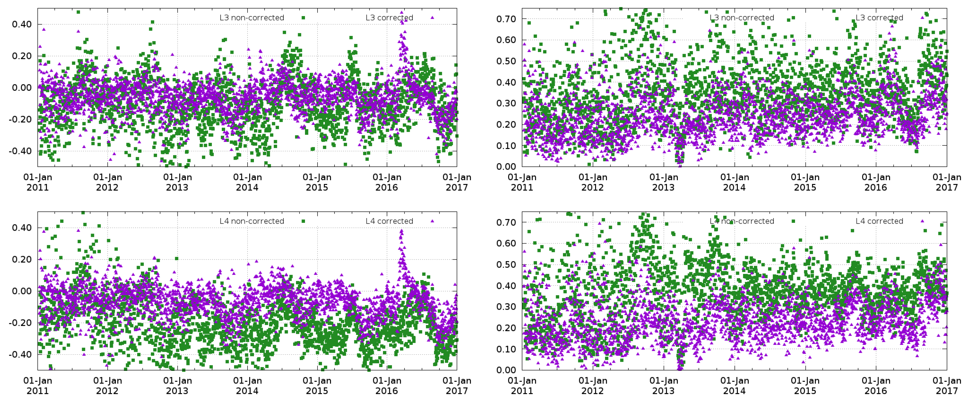
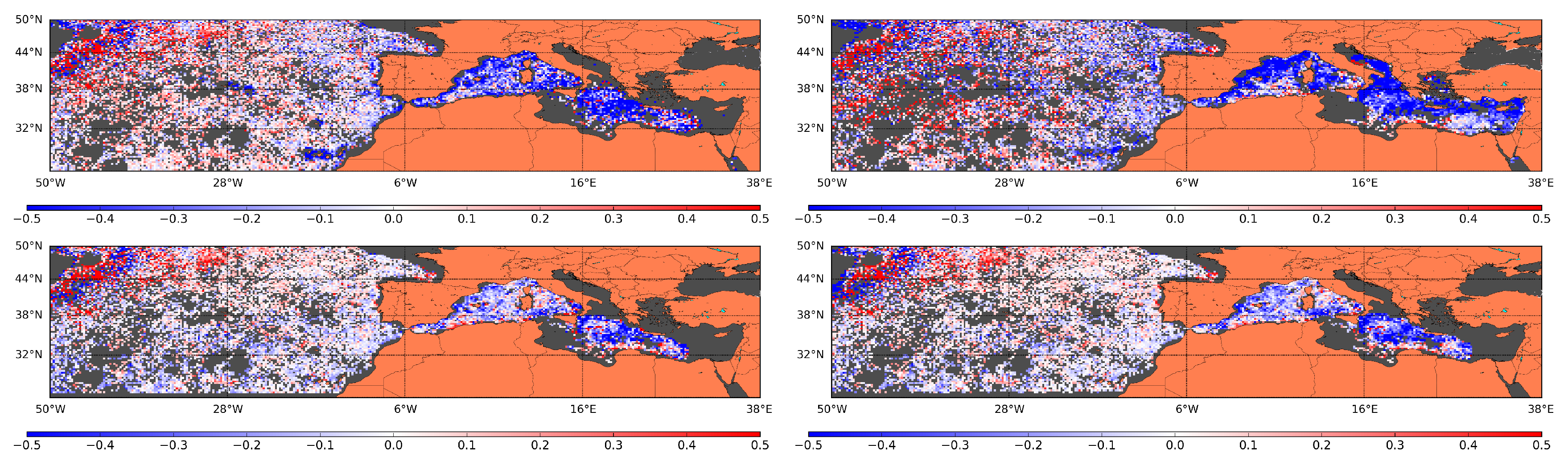
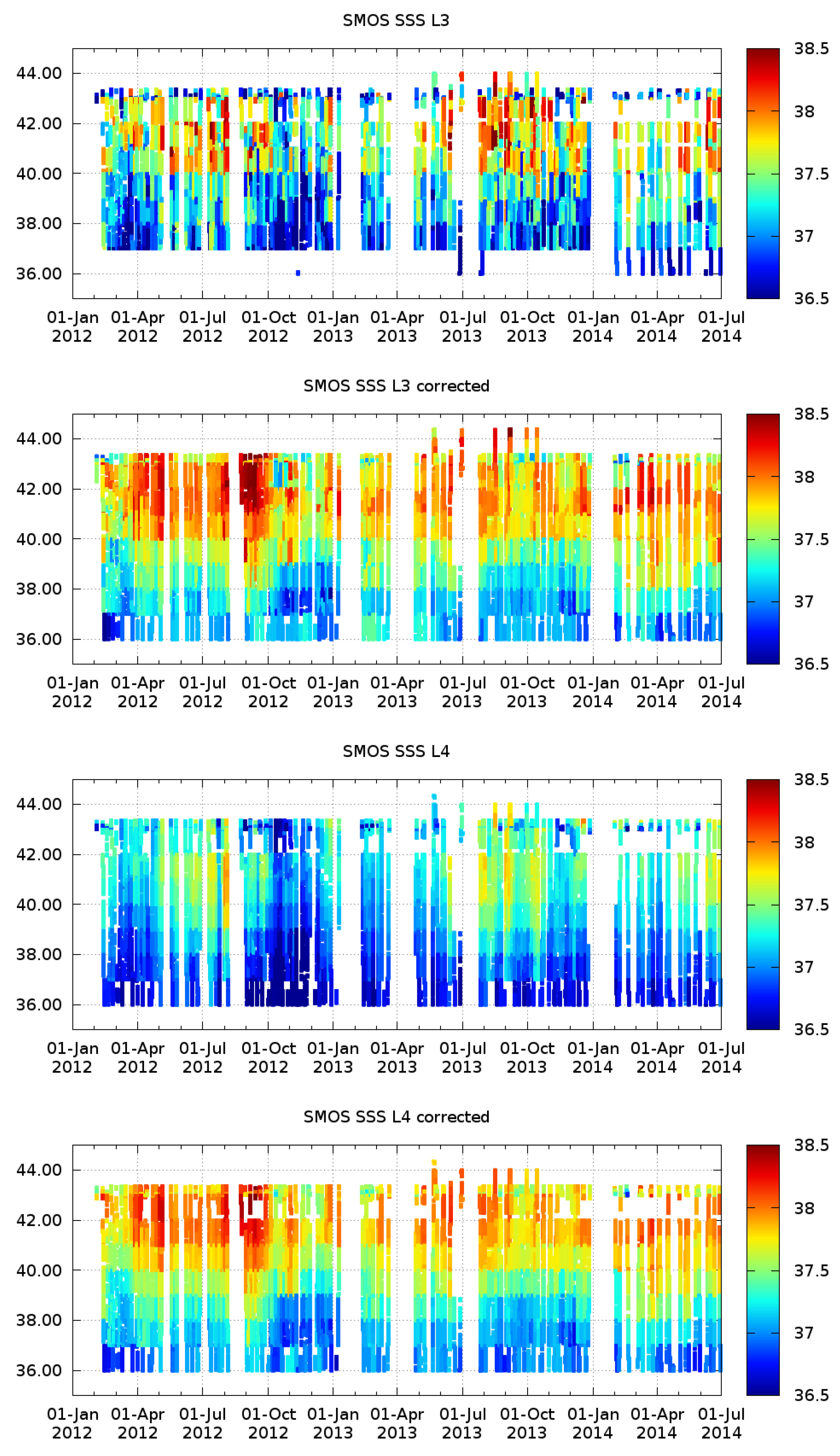
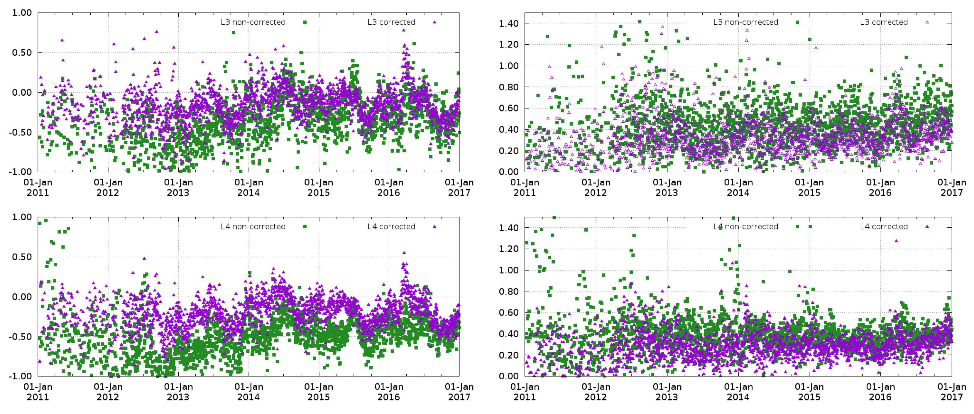
  • SMOS SSS L3 corrected products (L3 corrected): objectively analyzed 9-day maps at 0.25 × 0.25 resulting from the steps described in Section 3.1, Section 3.2 and Section 3.3.
  • SMOS SSS L3 products (L3): They are the global debiased non-Bayesian advanced products (see Section 2.1). They result from the methodologies described in Section 3.1 and Section 3.3. The unique difference with respect to the corrected L3 product is the time-bias correction. Instead of applying DINEOF decomposition, these products are time-bias corrected by assuming that the mean value of the SMOS-based anomaly at each map is null (see [20] for more details).
  • SMOS SSS L4 corrected products (L4 corrected): result from the multifractal fusion between the SMOS SSS L3 corrected maps and the OSTIA SST (step described in Section 3.4). They are provided at 0.05 × 0.05 on a daily basis.
  • SMOS SSS L4 products (L4): Multifractal fusion applied to the SMOS SSS L3 product (see Section 2.1).

4.1. Comparison with Argo Floats

Since we have used Argo floats for the generation of the time-dependent bias correction, this in situ data set is not an independent source of SSS data to be used in our assessment. However, we have included here a comparison with Argo not only for completeness, but also because our methodology uses the average in the full domain (North Atlantic and Mediterranean Sea) for removing the biases. We want to see here also the effect in the Mediterranean subdomain (which is the most challenging region in terms of processing). An independent validation is presented in the next sections. We also want to highlight that the number of Argo surface measurements available for validation in the Mediterranean Sea is low (less than 50) before 2014.
Thus, we will analyze the SMOS SSS errors with respect to Argo in two different regions:
  • Full domain (DOM), which includes part of the North Atlantic and the Mediterranean Sea and is defined in [ 26 , 50 ] N × [ 50 , 38 ] E
  • The Mediterranean Sea (MED) that is defined by the following rectangle [ 30 , 44 ] N × [ 6 , 30 ] E.
Figure 3 shows the time evolution of the mean difference between the L3 (green squares) and L3 corrected (violet triangles) products and Argo floats (plot in the first row and first column) in DOM and the corresponding standard deviation (in the plot of the second column in the first row of the same figure). As observed in the figure, the mean values of the differences of the L3 corrected product are closer to the 0 line than the ones of the L3 product. Additionally, the standard deviation of the difference corresponding to the L3 corrected product is lower than the one corresponding to the L3 product. The same plots for L4 products are shown in the lower row of Figure 3. The analysis of these plots leads to analogous conclusions. The corrected L4 reduces the errors with respect to the Argo measurements.
Figure 4 shows the same four plots as before but computed over the MED subdomain only. As in the case of the DOM, the corrected products are closer to the Argo measurements (both in bias and standard deviation). However, in this case, a seasonal bias is still present. Although the biases and the standard deviations in the Mediterranean basin have been noticeably reduced (see the numbers in Table 2), some residual (time-dependent) bias is still present.
Figure 5 and Figure 6 show the spatial distribution of the mean and standard deviation of the differences between the different SMOS SSS products and Argo. As observed in Figure 5, the major reduction of the bias is obtained in the Mediterranean basin, as well as the major reduction of the standard deviation (Figure 6). In particular, the SSS in the non-corrected products in the Northwestern Mediterranean are strongly biased, while the corrected ones strongly reduce the bias in this region.
In these figures, no noticeable differences between corrected L3 and L4 products are observed. We want to also highlight that the accuracy in the Eastern Mediterranean is very poor. The Eastern Mediterranean region is strongly affected by RFI and the SMOS SSS retrieval there is even more challenging. Recent calibration and image reconstruction techniques [34,47,48] are providing promising results in these more degraded regions.

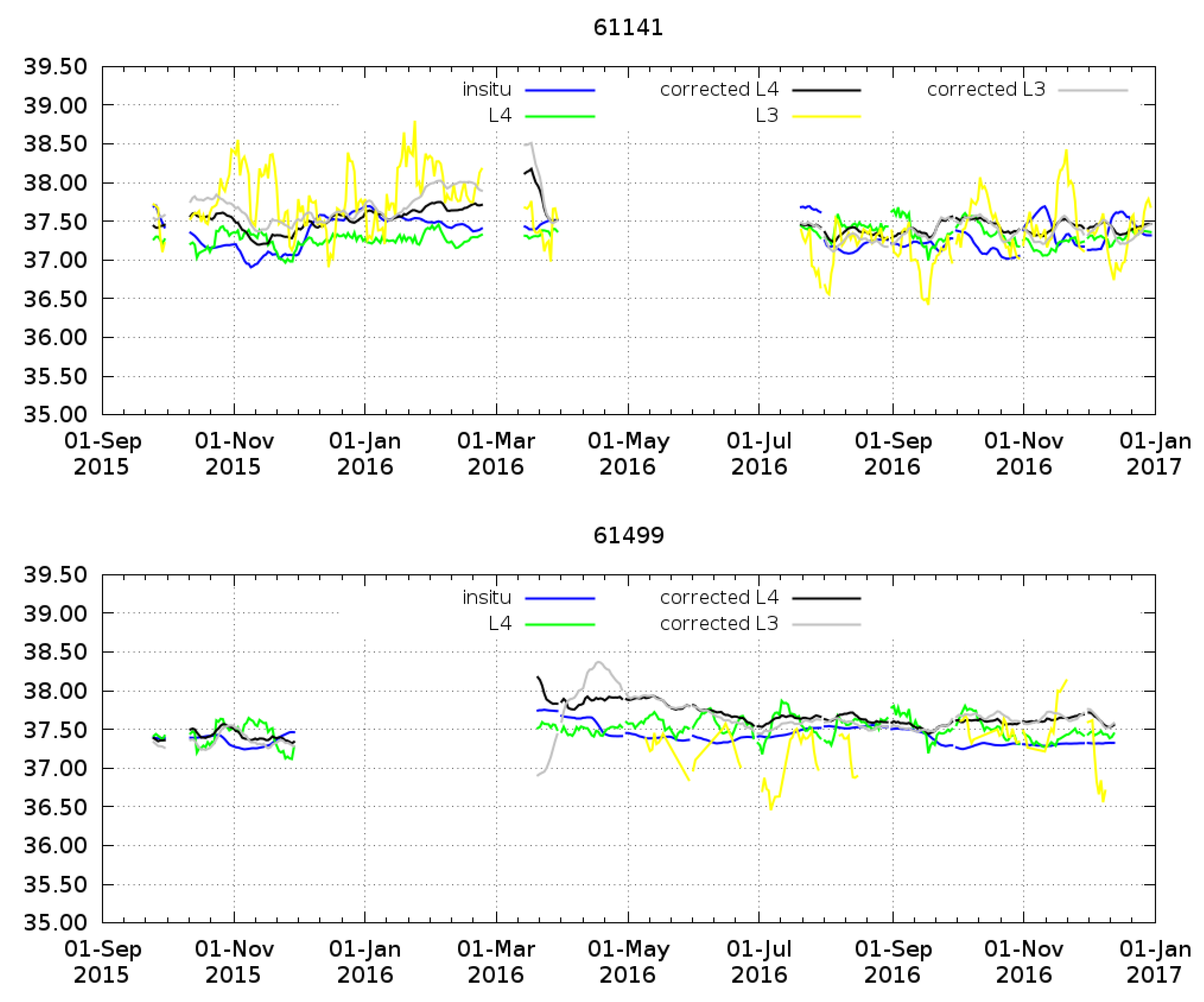
4.2. Comparison with Moorings Data

In this section, we have compared the time series of the six years of SMOS SSS with the time series provided by moorings located in the coastal Western Mediterranean (see their location in Figure 1).
The spatial and temporal scales corresponding to the mooring and satellite measured SSS are very different. While the satellite observations correspond to SSS over an area of 0.25 × 0.25 (or 0.05 × 0.05 in the case of L4 products) and computed from an integrated time period of nine days, the mooring measurements represent SSS values of a pinpointed location at hourly time steps. These differences are even more noticeable in regions with high mesoscale activity. For example, moorings number 61,198, 61,141 61,281 and 6120 are located very close to the Mediterranean continental Spanish coast (see Figure 1). These locations are strongly affected by the general circulation (old AW coming from the North), sometimes by recent (fresher) AW coming from the South, and episodically by continental fresh water discharges. These produce complex mixing dynamics that form filaments and mesoscale and submesoscale structures with strong SSS gradients and fast dynamics. This is even more problematic in the vicinity of the Alboran Sea (mooring number 61,198), where the SSS variability amplitude can reach 2PSU within hours. Thus, in order to make both SSS data sets more comparable, we have applied a slide averaging window of nine days to the mooring data. This smoothing technique does not completely solve the temporal scale differences in the comparison between mooring and satellite SSS (as we will discuss below).
Figure 7 shows the time series corresponding to the moorings anchored in the Ibiza Channel and the Palma Bahia (buoys number: 61,141 and 61,499, respectively, see their location in Figure 1). Time series corresponding to the moorings are plotted in blue, L3 in yellow, L3 corrected in grey, L4 in green and L4 corrected in black. The in situ salinity range is relatively narrow (<1PSU) in the case of these two Balearic moorings. In their case, the improvement in the corrected SMOS SSS is not evident because the initial values of the L4 products (and L3 to a lesser extent) are already close. Indeed, although spurious oscillations are also corrected, the mean salinity value of the non-corrected SMOS products seem to be closer to the in situ than the mean salinity values of the corrected SMOS products.
Figure 8 shows the time series corresponding to the four moorings anchored on the Spanish continental coast (moorings number 61,198, 61,417 61,281 and 61,280, see their locations in Figure 1), where the in situ salinity range is higher (>1 PSU). In this case, although a slide averaging window of nine days has been applied to the mooring data, the time series of these moorings (blue lines) still present jumps with a fast dynamics that will not be captured by the satellite. When these jumps are persistent (for example January 2013 mooring number 6147), the satellite captures the jump. However, if the jump does not lead to a persistent change of the SSS (for example January 2012 mooring number 61,198), the satellite will not capture the dynamics. In spite of the temporal scale limitations, as observed in Figure 8, both corrected products (grey and black points) are closer to the in situ (blue points) than the non-corrected ones (yellow and green).
Table 3 shows the mean and the standard deviation of the differences between SMOS SSS and in situ SSS. The comparison shows that, in general, we obtain a reduction of the bias that is more than two-fold for both L3 and L4. We also observe a reduction in the corrected SMOS SSS of the standard deviation. If we compare the results corresponding to the L3 corrected with the results corresponding to the L4 corrected products, the statistics are very similar. In general, a slight increase of the bias appears in the L4 product, which is compensated by a reduction of the standard deviation. In general, there is a residual negative bias still present in the corrected SMOS SSS products. The moorings anchored in the Baleares (61,141 and 61,499) have a different behaviour with respect to the rest of moorings. On one hand, the residual bias is positive. On the other hand, the bias in the Palma bahia (61,499) corresponding to the L4 corrected increases with respect to the bias of the L4 (as mentioned above).
This section shows that our corrections can improve the SMOS SSS retrieval over the whole range of salinity of the Western Mediterranean (36.5–38.5). However, the difference of residual offsets at the respective moorings locations has yet to be investigated.

4.3. Comparison with TRANSMED SSS

In situ data from the TRANSMED program have been also used as an independent source of SSS data for validating the resulting SMOS products. These data cover from February 2012 to July 2014 and they are composed of SSS and SST acquired underway along repeated transects at ∼3 m deep along the Western Mediterranean (see Figure 9).
Table 4 shows the statistics corresponding to the four different SMOS SSS products and the in situ SSS. The time correction proposed in this work reduces the bias in both products L3 and L4 from −0.54 PSU to less than −0.1 PSU. On the other hand, a reduction of 0.12 (0.03) PSU in the standard deviation of the L3 (and L4 respectively) is also obtained.
In order to take a global look at the spatial biases of the SMOS SSS product with respect to TRANSMED SSS data, Figure 10 shows a latitudinal Hovmöller diagram of the different SSS data ordered in time. Thus, on the top of the figure, the Hovmöller corresponding to TRANSMED SSS is shown; in the second row, the Hovmöller corresponding to the L3 SSS product; in the third row, the corresponding to the L3 corrected; in the fourth, the L4; and in the last row, the L4 corrected SMOS SSS product is shown. The Hovmöller corresponding to the non-corrected SMOS SSS products are contaminated by a strong negative bias (as observed also in the statistics of Table 4). Additionally, the time correction proposed in this work has strongly mitigated some particular events that contaminated the initial SMOS product. For instance, in October and November 2012, the non-corrected plots show SSS values lower than 37 PSU practically at all the latitudes, when such low SSS values are limited to recent AW and thus confined to the southernmost part of the basin, as shown by the TRANSMED SSS. The Hovmöller plots corresponding to the corrected products show on the contrary a more similar behavior than the ones observed by the TRANSMED SSS. A similar effect is observed in October 2013 and April 2014, where spurious fresh events contaminate all the latitude range in the non-corrected Hovmöller diagrams but not in the corrected nor in the TRANSMED diagrams. In spite of the different spatial scales, which produce a more pixelated plot for SMOS, and in spite of a slight global fresh bias, which also shows the statistics of Table 4, the corrected SMOS SSS products allow for reducing the spatial noise and they also improve the depiction of the North-South SSS gradients. For instance, the fresher (blue) area moves further north around October 2013 in the TRANSMED SSS and both corrected SMOS products, whereas in March–April 2014, the salty water moves south.
In the northern part of the basin, the comparison between corrected SMOS SSS products and TRANSMED SSS is impaired mostly by the Rhone river plume. Its scales of variability in both space (along the shoreline or offshoreward) and time (hours under wind influence or heavy precipitating events) cannot be captured by SMOS. Further analysis on larger scales (northwestern part of the basin, season) would probably help with assessing the freshwater discharges observed by SMOS in the Gulf of Lion.

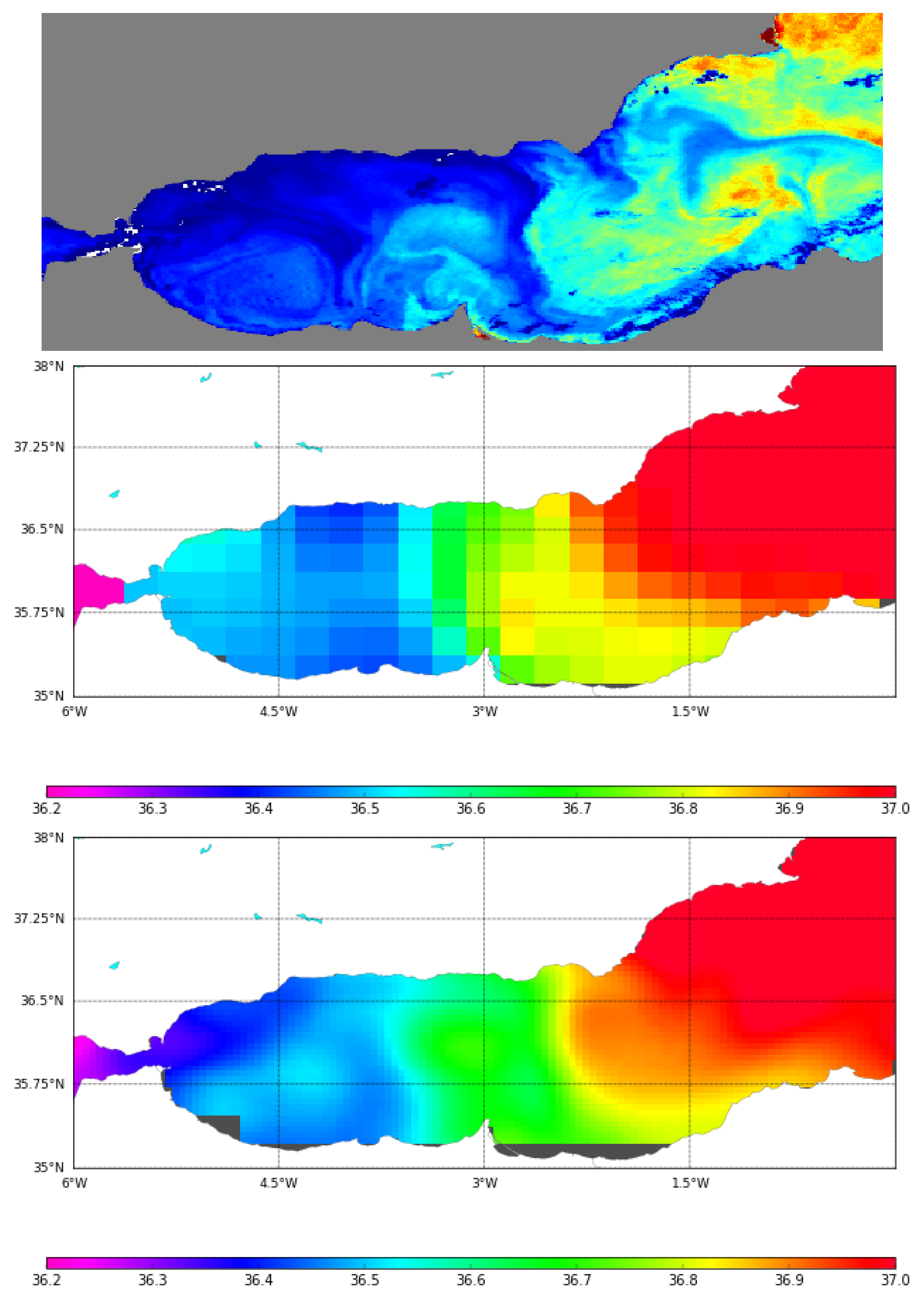
4.4. Spatial Structures: Qualitative Comparison with AVHRR Images

In the previous sections (Section 4.1, Section 4.2 and Section 4.3), we have shown that the corrected SMOS products have lower error than the non-corrected SMOS products (lower bias and std with respect to in situ measurements). However, the performances provided by the corrected L3 and L4 products in the comparison with in situ data are very similar. The main conclusions are that L3 typically provides a slightly lower bias, but L4 provides a slightly lower standard deviation. Therefore, the quality of both products as described by these metrics is very similar. In this section, we want to compare both SMOS SSS corrected products with high resolution AVHRR images in order to assess the kind of spatial structures that each one describes (i.e., which is the added value of the L4 SMOS corrected product with respect to the L3 SMOS corrected one). Therefore, this section is just a qualitative comparison. We want to stress that, although the L4 are computed by means of multifractal fusion with OSTIA SST maps, in this section, we have not considered OSTIA maps, but the AVHRR images as mentioned in Section 2.3.
In Figure 11, Figure 12 and Figure 13, AVHHR images of the Alboran Sea on 25 September of 2011, 1 March 2013 and 25 June 2014 are shown. In Figure 11, both Western (A) and Eastern (B) Alboran gyres are fully developed. Close to 1.5 W, a thermal front (C) clearly bounds the AW that enters into the Mediterranean. The corrected L3 SMOS SSS map also displays clearly the front close to the 1.5 W separating the Atlantic and the Mediterranean waters, and also recognizes the fresh water that enters from the Strait of Gibraltar. However, the spatial structure of the gyres is blurred. The corrected L4 SMOS SSS map shows clearly both gyres. In Figure 12, the Western gyre collapses. The spatial gradients shown by L4 SMOS SSS are not coherent this time, with the spatial structures shown by the AVHRR image. Indeed, during wintertime, AW is signified by higher SST (red for AW and blue for Mediterranean waters in AVHRR images). Thus, lower salinity values would have been expected in the Southern part of the SMOS SSS images, which is not the case. Until further investigations are carried out, it must be noted that gyres in the Alboran Sea are extremely variable in both space and time, and that comparison of SMOS data with instantaneous images has its limits.
In Figure 13, the Eastern gyre collapses. In this case, SMOS presents coherent values with what the AVHRR image is showing.
In Figure 14, the main feature of both the SMOS SSS L3 and L4 corrected maps is the frontal zone between the Atlantic and the Mediterranean waters north of the Baleares. Such a zonal gradient does not appear in the AVHRR image. The area of the Rhone river influence (A) is well marked on the three products, with colder SST and lower SSS west of 5 E in the gulf, and a tongue extending southward (the latter hardly visible though on the SMOS SSS L3 corrected map). A second colder plume extending southward off 6 E (B) in the AVHRR image also shows as a plume of lower SSS on the SMOS SSS L4 corrected map, but not on the SMOS SSS L3 corrected map.

5. Conclusions

A new methodology using a combination of the new retrieval debiased non-Bayesian algorithm, DINEOF and multifractal fusion has been used to obtain Sea Surface Salinity (SSS) fields over the North Atlantic Ocean and the Mediterranean Sea. The data used for the analysis is the 9-day 0.25 SMOS SSS L3 binned maps produced by the Barcelona Expert Centre (BEC), and it has been shown that the proposed methodology improves the accuracy with respect to the Objectively Analyzed maps and the L4 products that are currently being produced at the BEC. In particular, a reduction of the seasonal bias has been observed in the final data set as well as a reduction in the standard deviation of the error. The overall comparison of the new products with Argo floats provides an RMSE of 0.26 PSU in the full domain of study (North Atlantic and Mediterranean Sea) in comparison with an RSME of 0.41 PSU corresponding to the initial SMOS products. In the Mediterranean basin, the methodology also allows for reducing the error (0.39 PSU against 0.70 PSU in the case of the L4 products).
The comparison with the SSS TRANSMED in situ data shows that, in spite of the limitation of the differences in the spatial and temporal resolutions, the corrected SMOS SSS products not only provide a coherent description of the dynamics in the Algerian basin (as pointed out in [19]), but also a coherent description of the Balearic frontal zone. The short time and space scales of the freshwater discharges impair the detection of the latter by the SMOS SSS products, as seen in the gulf of Lion. An analysis at the seasonal scale might improve the comparison in this region. On the other hand, the L4 corrected products provide a description of the mesoscale salinity in regions so challenging as the Alboran Sea, where the water is surrounded by land a few kilometers away, and, therefore, the land sea contamination is especially strong.
The use of the DINEOF decomposition in combination to these new debiased non-Bayesian techniques has a high potential for improving the quality of the SMOS SSS maps not only in the Mediterranean, but also in other regions. On one hand, the debiased non-Bayesian approach mitigates the systematic biases (constant on time) like the land-sea contamination. In addition, its statistical filtering criteria improve the coverage with respect to official Level 2 Ocean Salinity products. On the other hand, the EOF decomposition allows for the characterization of the time-dependent biases. One of the major benefits of using EOFs decomposition in this context is that the technique not only allows to characterize the time-dependent biases with a regular (seasonal) bias (which is still an issue in the SMOS products, [49]), but the technique also allows the removal of some particular events, which could be caused by strong RFI. For example, in this study, we have shown that the proposed methodology has removed the spurious fresh event that contaminated the Mediterranean basin in October–November 2012. In addition, the use of multifractal fusion allows for improving the spatial resolutions and describing better the mesoscale dynamics.
Despite the encouraging results, there is still significant room for improvement. For instance, the EOFs to be removed should not be chosen one by one but as a single, optimized combination. This means assuming that the time-dependent bias is captured not by a single EOF, but by a combination of them. On the other hand, we have applied here a multifractal fusion scheme that is scalar, and more complex schemes can be investigated and tested in the Mediterranean.
All in all, this work has shown that these techniques are not only beneficial, but required to fully correct the SMOS SSS retrievals in some particular regions. Because of the capability of the combined debiased non-Bayesian retrieval-DINEOF-fusion approach to detect biases and reduce other sources of noise and error from the SMOS SSS data, the application of this technology to enclosed seas suffering from strong sources of contamination, such as the China Sea, the Baltic Sea and the Black Sea, will potentially provide promising results.

Acknowledgments

This work has been carried out within the project “SMOS sea surface salinity data in the Mediterranean Sea” ([50]), funded by the European Space Agency “Support to Science (STSE) PATHFINDERS” call. Part of this work was also supported by the Ministry of Economy and Competitiveness, Spain, through the National R+D Plan under L-Band Project ESP2017-89463-C3-1-R, PROMISES Project ESP2015-67549-C3 and previous grants. Argo data were collected and made freely available by the international Argo project and the national programs that contribute to it [51]. SSS time series from the moorings located in the Western Mediterranean were collected and made freely available by the Copernicus project and the programs that contribute to it (available online: [25] (accessed on 19 March 2018) and available online: [26] (accessed on 8 May 2012).). The TRANSMED system (available online: [29] (accessed on 19 March 2018)) was first fostered by the Commission Internationale pour l’Exploration de la Méditerranée, the Science Commission (CIESM) under the program TRANSMED/PartnerSHIPs (available online: [52] (accessed on 19 March 2018)), and achieved thanks to the support of the INSU MISTRALS /HyMeX program. The involvement of Gilles Rougier, the MIO’s staff and from the DT INSU, and the longstanding support of the maritime companies Linea Messina (Genoa, Italy) and Marfret (Marseille, France) have been pivotal to the TRANSMED data collection. This work is a contribution to the ANR ASICS-MED project (grant ANR-12-BS06-0003). The MIO laboratory acknowledges the support received from the European FEDER Fund under project 1166-39417. OSTIA SST data were provided by GHRSST, UKMO and CMEMS.

Author Contributions

Estrella Olmedo, Aida Alvera-Azcárate and Antonio Turiel conceived and designed the algorithm for the SMOS SSS products generation. Estrella Olmedo and Aida Alvera-Azcárate implemented the new algorithm. Estrella Olmedo and Isabelle Taupier-Letage performed the validation of the new SMOS SSS product. Isabelle Taupier-Letage conducted the oceanographic interpretation of the results. The manuscript was prepared by Estrella Olmedo. All authors revised and approved the final manuscript.

Conflicts of Interest

The authors declare no conflict of interest.

References

  1. Giorgi, F. Climate change hot-spots. Geophys. Res. Lett. 2006, 33, L08707. [Google Scholar] [CrossRef]
  2. Millot, C.; Taupier-Letage, I. Circulation in the Mediterranean Sea. In The Handbook of Environmental Chemistry, 5 Part K; Saliot, A., Ed.; Springer: Berlin/Heidelberg, Germany, 2005; pp. 29–66. Available online: https://hal.archives-ouvertes.fr/hal-01191856 (accessed on 23 January 2018). [CrossRef] [Green Version]
  3. Taupier-Letage, I.; Puillat, I.; Millot, C.; Raimbault, P. Biological response to mesoscale eddies in the Algerian Basin. J. Geophys. Res. Oceans 2003, 108, 3245. [Google Scholar] [CrossRef]
  4. Isern-Fontanet, J.; Font, J.; Garcia-Ladona, E.; Emelianov, M.; Millot, C.; Taupier-Letage, I. Spatial structure of anticyclonic eddies in the Algerian basin (Mediterranean Sea) analyzed using the Okubo-Weiss parameter. Deep Sea Res. II 2004, 51, 3009–3028. [Google Scholar] [CrossRef]
  5. Schroeder, K.; Garcìa-Lafuente, J.; Josey, S.; Artale, V.; Buongiorno-Nardelli, B.; Carrillo, A.; Gacic, M.; Gasparin, G.; Herrmann, M.; Lionello, P.; et al. Circulation of the Mediterranean Sea and its variability. In The Climate of the Mediterranean Region; Lionello, P., Ed.; Elsevier: Oxford, UK, 2012; pp. 187–256. [Google Scholar]
  6. Estournel, C.; Testor, P.; Damien, P.; D’ortenzio, F.; Marsaleix, P.; Conan, P.; Prieur, L. High resolution modelling of dense water formation in the north-western Mediterranean during winter 2012–2013: Processes and budget. J. Geophys. Res. Oceans 2016, 121, 5367–5392. [Google Scholar] [CrossRef]
  7. Waldman, R.; Somot, S.; Herrmann, M.; Testor, P.; Estournel, C.; Sevault, F.; Prieur, L.; Mortier, L.; Coppola, L.; Taillandier, V.; et al. Estimating dense water volume and its evolution for the year 2012–2013 in the Northwestern Mediterranean Sea: An observing system simulation experiment approach. J. Geophys. Res. Oceans 2016, 121, 6696–6716. [Google Scholar] [CrossRef]
  8. HYMEX (HYdrological Cycle in the Mediterranean EXperiment). Available online: https://www.hymex.org/ (accessed on 23 January 2018).
  9. Drobinski, P.; Ducrocq, V.; Allen, J.; Alpert, P.; Anagnostou, E.; Béranger, K.; Borga, M.; Braud, I.; Chanzy, A.; Davolio, S.; et al. HyMeX, a 10-year multidisciplinary project on the Mediterranean water 1 cycle. Bull. Am. Meteorol. Soc. 2014, 95, 1063–1082. [Google Scholar] [CrossRef]
  10. Somot, S.; Sevault, F.; Déqué, M.; Crépon, M. 21st century climate change scenario for the Mediterranean using a coupled atmosphere-ocean regional climate model. Glob. Planet. Change 2008, 63, 112–126. [Google Scholar] [CrossRef] [Green Version]
  11. Adloff, F.; Somot, S.; Sevault, F.; Jordà, G.; Aznar, R.; Déqué, M.; Herrmann, M.; Marcos, M.; Dubois, C.; Padorno, E.; et al. Mediterranean Sea response to climate change in an ensemble of twenty first century scenarios. Clim. Dyn. 2015, 45, 2775–2802. [Google Scholar] [CrossRef]
  12. Somot, S.; Houpert, L.; Sevault, F.; Testor, P.; Bosse, A.; Taupier-Letage, I.; Bouin, M.; Waldman, R.; Cassou, C.; Sanchez-Gomez, E.; et al. Characterizing, modelling and understanding the climate variability of the deep water formation in the North-Western Mediterranean Sea. Clim. Dyn. 2016, 1–32. [Google Scholar] [CrossRef]
  13. Herrmann, M.; Diaz, F.; Estournel, C.; Marsaleix, P.; Ulses, C. Impact of atmospheric and oceanic interannual variability on the Northwestern Mediterranean Sea pelagic planktonic ecosystem and associated carbon cycle. J. Geophys. Res. Oceans 2013, 118, 5792–5813. [Google Scholar] [CrossRef]
  14. Herrmann, M.; Estournel, C.; Diaz, F.; Adloff, F. Impact of climate change on the Northwestern Mediterranean Sea pelagic planktonic ecosystem and associated carbon cycle. J. Geophys. Res. Oceans 2014, 119, 5815–5836. [Google Scholar] [CrossRef]
  15. Mecklenburg, S.; Drusch, M.; Kerr, Y.H.; Font, J.; Martin-Neira, M.; Delwart, S.; Buanadicha, G.; Reul, N.; Daganzo-Eurebio, E.; Oliva, R.; et al. ESA’s Soil Moisture and Ocean Salinity Mission: Mission Performance and Operations. IEEE Trans. Geosci. Remote Sens. 2012, 50, 1354–1366. [Google Scholar] [CrossRef] [Green Version]
  16. Font, J.; Camps, A.; Borges, A.; Martín-Neira, M.; Boutin, J.; Reul, N.; Kerr, Y.; Hahne, A.; Mecklenburg, S. SMOS: The Challenging Sea Surface Salinity Measurement From Space. Proc. IEEE 2010, 98, 649–665. [Google Scholar] [CrossRef] [Green Version]
  17. Kerr, Y.; Waldteufel, P.; Wigneron, J.; Delwart, S.; Cabot, F.; Boutin, J.; Escorihuela, M.; Font, J.; Reul, N.; Gruhier, C.; et al. The SMOS mission: New tool for monitoring key elements of the global water cycle. Proc. IEEE 2010, 98, 666–687. [Google Scholar] [CrossRef] [Green Version]
  18. Alvera-Azcárate, A.; Barth, A.; Parard, G.; Beckers, J. Analysis of SMOS sea surface salinity data using DINEOF. Remote Sens. Environ. 2016, 180, 137–145. [Google Scholar] [CrossRef]
  19. Isern-Fontanet, J.; Olmedo, E.; Turiel, A.; Ballabrera-Poy, J.; García--Ladona, E. Retrieval of eddy dynamics from SMOS sea surface salinity measurements in the Algerian Basin (Mediterranean Sea). Geophys. Res. Lett. 2016, 43, 6427–6434. [Google Scholar] [CrossRef]
  20. Olmedo, E.; Martínez, J.; Turiel, A.; Ballabrera-Poy, J.; Portabella, M. Debiased non-Bayesian retrieval: A novel approach to SMOS Sea Surface Salinity. Remote Sens. Environ. 2017, 193, 103–126. [Google Scholar] [CrossRef]
  21. Olmedo, E.; Martínez, J.; Umbert, M.; Hoareau, N.; Portabella, M.; Ballabrera-Poy, J.; Turiel, A. Improving time and space resolution of SMOS salinity maps using multifractal fusion. Remote Sens. Environ. 2016, 180, 246–263. [Google Scholar] [CrossRef]
  22. ESA. Available online: https://earth.esa.int/web/guest/-/level-1b-full-polarization-6889 (accessed on 23 January 2018).
  23. Global SMOS SSS Maps. Available online: http://bec.icm.csic.es/ocean-experimental-dataset-global/ (accessed on 23 January 2018).
  24. Puertos del Estado. Available online: http://www.puertos.es (accessed on 23 January 2018).
  25. Copernicus Marine Environment Monitoring Service. Available online: http://marine.copernicus.eu (accessed on 23 January 2018).
  26. OceanSITES. Available online: http://www.oceansites.org (accessed on 23 January 2018).
  27. SOCIB. Available online: http://www.socib.eu/?seccion=observingFacilities&facility=mooring&id=146 (accessed on 23 January 2018).
  28. SOCIB. Available online: http://www.socib.eu/?seccion=observingFacilities&facility=mooring&id=143 (accessed on 23 January 2018).
  29. TRANSMED. Available online: http://www.mio.univ-amu.fr/?TRANSMED (accessed on 23 January 2018).
  30. Taupier-Letage, I.; Bachelier, C.; Rougier, G. Thermosalinometer TRANSMED, Marfret Niolon, definitive data set. SEDOO OMP 2014. [Google Scholar] [CrossRef]
  31. Donlon, C.J.; Martin, M.; Stark, J.; Roberts-Jones, J.; Fiedler, E.; Wimmer, W. The operational Sea Surface Temperature and Sea Ice Analysis (OSTIA) system. Remote Sens. Environ. 2012, 116, 140–158. [Google Scholar] [CrossRef]
  32. MIO. Available online: www.ifremer.fr/osis_2014 (accessed on 19 March 2018).
  33. Taupier-Letage, I. On the use of thermal infrared images for circulation studies: Applications to the eastern Mediterranean basin. In Remote Sensing of the European Seas; Barale, V., Gade, M., Eds.; Springer: Berlin/Heidelberg, Germany, 2008; Available online: https://hal.archives--ouvertes.fr/hal--01196705 (accessed on 23 January 2018).
  34. González-Gambau, V.; Olmedo, E.; Turiel, A.; Martínez, J.; Ballabrera-Poy, J.; Portabella, M.; Piles, M. Enhancing SMOS brightness temperatures over the ocean using the nodal sampling image reconstruction technique. Remote Sens. Environ. 2016, 180, 202–220. [Google Scholar] [CrossRef]
  35. Zweng, M.; Reagan, J.; Antonov, J.; Locarnini, R.; Mishonov, A.; Boyer, T.; Garcia, H.; Baranova, O.; Johnson, D.; Seidov, D.; et al. World Ocean Atlas 2013, Volume 2: Salinity; Levitus, A., Ed.; Mishonov Technical; NOAA: Silver Spring, MD, USA, 2013; pp. 39–74. [Google Scholar]
  36. Beckers, J.M.; Rixen, M. EOF calculations and data filling from incomplete oceanographic data sets. J. Atmos. Ocean. Technol. 2003, 20, 1839–1856. [Google Scholar] [CrossRef]
  37. Alvera-Azcárate, A.; Barth, A.; Rixen, M.; Beckers, J.M. Reconstruction of incomplete oceanographic data sets using Empirical Orthogonal Functions. Application to the Adriatic Sea surface temperature. Ocean Model. 2005, 9, 325–346. [Google Scholar] [CrossRef] [Green Version]
  38. Alvera-Azcárate, A.; Barth, A.; Sirjacobs, D.; Beckers, J.M. Enhancing temporal correlations in EOF expansions for the reconstruction of missing data using DINEOF. Ocean Sci. 2009, 5, 475–485. [Google Scholar] [CrossRef]
  39. Alvera-Azcárate, A.; Barth, A.; Beckers, J.M.; Weisberg, R.H. Multivariate Reconstruction of Missing Data in Sea Surface Temperature, Chlorophyll and Wind Satellite Fields. J. Geophys. Res. 2007, 112, C03008. [Google Scholar] [CrossRef]
  40. Nechad, B.; Ruddick, K.; Park, Y. Calibration and validation of a generic multisensor algorithm for mapping of total suspended matter in turbid waters. Remote Sens. Environ. 2010, 114, 854–866. [Google Scholar] [CrossRef]
  41. Alvera-Azcárate, A.; Vanhellemont, Q.; Ruddick, K.; Barth, A.; Beckers, J.M. Analysis of high frequency geostationary ocean colour data using DINEOF. Estuar. Coast. Shelf Sci. 2015, 159, 28–36. [Google Scholar] [CrossRef]
  42. Turiel, A.; Solé, J.; Nieves, V.; Ballabrera-Poy, B.; García-Ladona, E. Tracking oceanic currents by singularity analysis of Microwave Sea Surface Temperature images. Remote Sens. Environ. 2008, 112, 2246–2260. [Google Scholar] [CrossRef]
  43. Isern-Fontanet, J.; García-Ladona, E.; Font, J. Microcanonical multifractal formalism: Application to the estimation of ocean surface velocities. J. Geophys. Res. 2007, 112, 2156–2202. [Google Scholar] [CrossRef]
  44. Nieves, V.; Llebot, C.; Turiel, A.; Solé, J.; García-Ladona, E.; Estrada, M.; Blasco, D. Common turbulent signature in sea surface temperature and chlorophyll maps. Geophys. Res. Lett. 2007, L23602. [Google Scholar] [CrossRef]
  45. Umbert, M.; Hoareau, N.; Turiel, A.; Ballabrera-Poy, J. New blending algorithm to synergize ocean variables: The case of SMOS sea surface salinity maps. Remote Sens. Environ. 2014, 146, 188–200. [Google Scholar] [CrossRef]
  46. Hernández-Carrasco, I.; Sudre, J.; Garcon, V.; Yahia, H.; Garbe, C.; Paulmier, A.; Dewitte, B.; Illig, S.; Dadou, I.; González-Dávila, M.; et al. Reconstruction of super-resolution ocean pco2 and airsea fluxes of co2 from satellite imagery in the southeastern atlantic. Biogeosciences 2015, 12, 5229–5245. [Google Scholar] [CrossRef]
  47. González-Gambau, V.; Turiel, A.; Olmedo, E.; Martínez, J.; Corbella, I.; Camps, A. Nodal Sampling: A New Image Reconstruction Algorithm for SMOS. IEEE Trans. Geosci. Remote Sens. 2016, 54, 2314–2328. [Google Scholar] [CrossRef]
  48. González-Gambau, V.; Olmedo, E.; Martínez, J.; Turiel, A.; Duran, I. Improvements on Calibration and Image Reconstruction of SMOS for Salinity Retrievals in Coastal Regions. IEEE J. Sel. Top. Appl. Earth Obs. Remote Sens. 2017, 10, 3064–3078. [Google Scholar] [CrossRef]
  49. Martín-Neira, M.; Oliva, R.; Corbella, I.; Torres, F.; Duffo, N.; Durán, I.; Kainulainen, J.; Closa, A.; Zurita, A.; Cabot, F.; et al. SMOS Instrument performance and calibration after 5 years in orbit. Remote Sens. Environ. 2016, 180, 19–39. [Google Scholar] [CrossRef]
  50. DINEOF Analysis of SMOS Sea Surface Salinity Data. Available online: http://www.gher.ulg.ac.be/WP/ (accessed on 23 January 2018).
  51. Argo. Argo float data and metadata from Global Data Assembly Centre (Argo GDAC). SEANOE 2000. [Google Scholar] [CrossRef]
  52. CIESM. Available online: www.ciesm.org/marine/programs/partnerships.htm (accessed on 23 January 2018).
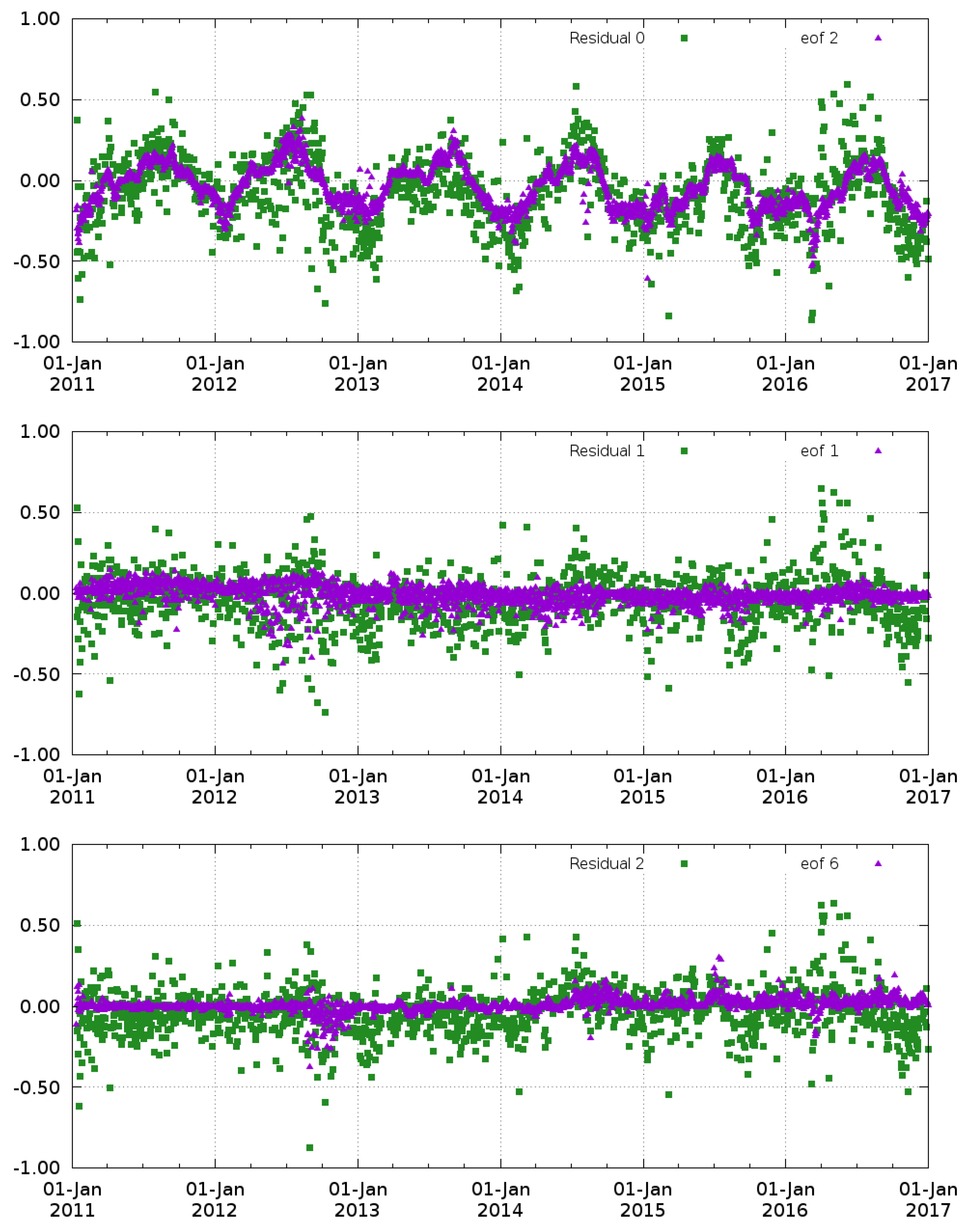
Figure 1. Location of the moorings that have been used for validation.
Remotesensing 10 00485 g001
Figure 2. Time evolution of the mean difference between SMOS and Argo SSS ( ϵ ( t ) green squares) and the contribution to the SSS of the EOF, which provides the largest correlation with the residual ( ω ( t ) violet triangles). On the top the results corresponding to the first iteration step; in the middle, the ones corresponding to the second iteration; and, in the bottom, the results of the third and last iteration.
Remotesensing 10 00485 g002
Figure 3. Time evolution of the mean differences (left) and standard deviation of the differences (right) between SMOS and Argo SSS computed over the full domain of the study. The top results correspond to the L3 products. The bottom results correspond to the L4 products. The non-corrected SMOS values are plotted with green squares and the corrected ones with violet triangles.
Remotesensing 10 00485 g003
Figure 4. As in Figure 3 but for the Mediterranean Sea (MED subdomain).
Remotesensing 10 00485 g004
Figure 5. Spatial distribution of the differences between SMOS and Argo SSS. In the first row, the plots correspond to the non-corrected products (left L3 and right L4). In the second row, the plots correspond to the corrected products (left L3 and right L4).
Remotesensing 10 00485 g005
Figure 6. Spatial distribution of the standard deviation of the differences between SMOS and Argo SSS. In the first row, the plots correspond to the non-corrected products (left L3 and right L4). In the second row, the plots correspond to the corrected products (left L3 and right L4).
Remotesensing 10 00485 g006
Figure 7. Moorings in the Ibiza Channel (top) and Palma bahia (bottom). Time evolution of the salinity: in blue the in situ SSS; L3 SMOS SSS in yellow; L4 SMOS SSS in green; corrected L3 SMOS SSS in grey; and corrected L4 SMOS SSS in black. The location of the buoys is shown in Figure 1.
Remotesensing 10 00485 g007
Figure 8. Moorings on the Spanish continental Mediterranean coast. Time evolution of the salinity: in blue the in situ SSS; L3 SMOS SSS in yellow; L4 SMOS SSS in green; corrected L3 SMOS SSS in grey; and corrected L4 SMOS SSS in black. The location of the buoys is shown in Figure 1.
Remotesensing 10 00485 g008
Figure 9. TRANSMED routes between 2012 and 2014.
Remotesensing 10 00485 g009
Figure 10. Latitudinal Hovmöller with the SSS values ordered in time: the first row corresponds to the TRANSMED SSS; the second row, the L3 SSS; the third row, L3 corrected; the fourth row, the L4; and the fifth shows the L4 corrected SMOS SSS values.
Remotesensing 10 00485 g010aRemotesensing 10 00485 g010b
Figure 11. Images of the Alboran Sea on 25th September 2011 as observed by AVHRR satellite (top); the SMOS SSS L3 corrected product; and the SMOS SSS L4 corrected product.
Remotesensing 10 00485 g011aRemotesensing 10 00485 g011b
Figure 12. Images of the Alboran Sea on 1st March 2013 as observed by AVHRR satellite (top); the SMOS SSS L3 corrected product; and the SMOS SSS L4 corrected product.
Remotesensing 10 00485 g012
Figure 13. Images of the Alboran Sea on 25th June 2014 as observed by AVHRR satellite (top); the SMOS SSS L3 corrected product; and the SMOS SSS L4 corrected product.
Remotesensing 10 00485 g013
Figure 14. Images of the Gulf of Lion and Balearic Front on 28th September 2011 as observed by AVHRR satellite (top); the SMOS SSS L3 corrected product; and the SMOS SSS L4 corrected product.
Remotesensing 10 00485 g014aRemotesensing 10 00485 g014b
Table 1. Results of the first 10 iterations from the time-dependent bias deletion from EOF decomposition. The first column shows the residual remaining in each iteration. In the second column, the number of the EOF that provides the largest correlation with the residual in each step. The correlation between the different EOFs contributions to the SMOS SSS and the time-dependent bias is shown in the fifth column. In the third and fourth columns, the mean and standard deviation (respectevely) of the residual error before the correction.
ResidualEOF with Largest CorrelationCorrelationMeanStd
ϵ 0 20.69−0.070.23
ϵ 1 = ϵ 0 ω 2 10.46−0.040.17
ϵ 2 = ϵ 1 ω 1 60.27−0.030.15
ϵ 3 = ϵ 2 ω 6 30.28−0.050.15
ϵ 4 = ϵ 3 ω 3 50.31−0.040.14
ϵ 5 = ϵ 4 ω 5 70.21−0.050.14
ϵ 6 = ϵ 5 ω 7 80.20−0.050.14
ϵ 7 = ϵ 6 ω 8 40.19−0.050.13
ϵ 8 = ϵ 7 ω 4 270.17−0.050.13
ϵ 9 = ϵ 8 ω 27 90.16−0.050.13
Table 2. Statistics of the differences between SMOS and Argo SSS. For each of the four SMOS SSS products, the mean, the standard deviation and the root mean squared are shown. The statistics are computed over two different domains: first row: DOM, which contains the Mediterranean Sea and part of the North Atlantic; and the second row: MED, which contains the Mediterranean Sea only.
L3L3 CorrectedL4L4 Corrected
meanstdrmsmeanstdrmsmeanstdrmsmeanstdrms
DOM−0.120.350.41−0.060.240.26−0.200.380.46−0.070.230.26
MED−0.400.450.67−0.160.340.43−0.500.400.70−0.190.290.39
Table 3. Differences between SMOS and in situ SSS. For each one of the four SMOS products, the mean and the standard deviation are shown. In the first column the mooring ID is shown.
Mooring IDL3L3 CorrectedL4L4 Corrected
meanstdmeanstdmeanstdmeanstd
61,198−0.500.40−0.200.31−0.460.35−0.250.32
61,417−0.520.49−0.190.44−0.460.46−0.260.42
61,1410.200.480.200.280.030.240.140.20
61,4990.220.320.200.270.090.170.230.15
61,281−0.510.56−0.220.38−0.730.36−0.270.34
61,280−0.380.43−0.210.25−0.660.34−0.220.22
Table 4. Differences between SMOS and TRANSMED SSS values. For each one of the four SMOS SSS products, the mean, the standard deviation and the total number of colocations between in situ and satellite used in the statistics are provided.
L3L3 CorrectedL4L4 Corrected
Mean−0.54−0.03−0.54−0.09
Std0.390.270.280.25
Nmeas75,12997,5308815091,113

