On Signal Modeling of Moon-Based Synthetic Aperture Radar (SAR) Imaging of Earth


1
State Key Laboratory of Remote Sensing Science, Institute of Remote Sensing and Digital Earth, Chinese Academy of Sciences, Beijing 100101, China
2
University of Chinese Academy of Sciences, Beijing 100049, China
*
Author to whom correspondence should be addressed.
Remote Sens. 2018, 10(3), 486; https://doi.org/10.3390/rs10030486
Submission received: 26 December 2017
/
Revised: 14 March 2018
/
Accepted: 19 March 2018
/
Published: 20 March 2018
(This article belongs to the Special Issue Radar Imaging Theory, Techniques, and Applications)
Abstract
:The Moon-based Synthetic Aperture Radar (Moon-Based SAR), using the Moon as a platform, has a great potential to offer global-scale coverage of the earth’s surface with a high revisit cycle and is able to meet the scientific requirements for climate change study. However, operating in the lunar orbit, Moon-Based SAR imaging is confined within a complex geometry of the Moon-Based SAR, Moon, and Earth, where both rotation and revolution have effects. The extremely long exposure time of Moon-Based SAR presents a curved moving trajectory and the protracted time-delay in propagation makes the “stop-and-go” assumption no longer valid. Consequently, the conventional SAR imaging technique is no longer valid for Moon-Based SAR. This paper develops a Moon-Based SAR theory in which a signal model is derived. The Doppler parameters in the context of lunar revolution with the removal of ‘stop-and-go’ assumption are first estimated, and then characteristics of Moon-Based SAR imaging’s azimuthal resolution are analyzed. In addition, a signal model of Moon-Based SAR and its two-dimensional (2-D) spectrum are further derived. Numerical simulation using point targets validates the signal model and enables Doppler parameter estimation for image focusing.

1. Introduction
Earth observation from remote sensing satellites orbiting in a low Earth orbit provides a continuous stream of data that can enable a better understanding of the Earth with respect to climate change [1]. Recently, the concept of observing the Earth from the Moon-based platform was proposed [2,3,4]. The Moon, as the Earth’s only natural satellite, is stable in periodic motion, making an onboard sensor unique in observing large-scale phenomena that are related to the Earth’s environmental change [5,6]. Synthetic aperture radar (SAR), an active sensor, provides effective monitoring of the Earth with all-time observation capabilities [7,8].
A SAR placed in the lunar platform was proposed [3], in which the configurations and performance of The Moon-Based SAR system was thoroughly investigated. Also, the concept of the Moon-based Interferometric SAR (InSAR) were analyzed by Renga and Moccia [4]. Later, the performance and potential applications of the Moon-Based SAR were characterized by Moccia and Renga [5], and the scientific and technical issues in the application of lunar-based repeat track and along track interferometry in [6]. Following this stream of development, an L-band Moon-Based SAR for monitoring large-scale phenomena related to global environmental changes was discussed [9] and the coverage performance of the Moon-based platform for global change detection [10]. The geometric modeling and coverage for a lunar-based observation by using Jet Propulsion Laboratory (JPL) ephemerides data were addressed in [11]. These studies are focused on the performance analysis and potential applications with some assumptions, such as a regular spherical Earth, an orbicular circular lunar orbit, a fixed earth’s rotational velocity, and a stationary Moon. By so doing, the SAR onboard Moon can be viewed as an inverse SAR (ISAR) or an equivalent sliding spotlight SAR [6,12].
However, when the effect of the lunar revolution was ignored in modeling the Doppler parameters, SAR image focusing is degraded to certain extent. Another aspect is that the imaging geometry of the Moon-Based SAR is quite different from that of LEO SAR systems. For an extremely long synthetic aperture, the signal path is a curved trajectory, and the common ‘stop-and-go’ assumption is no longer valid due to the long delay time in wave propagation.
This paper aims at deriving a signal model of Moon-Based SAR imaging by considering the more complete, but more complex, geometry of SAR in Moon-Earth orbits. The Doppler parameters are first derived without assuming the ‘stop-and-go’ mode. The paper is organized as follows. In the next section, a right-handed Earth-centered reference coordinate is established to unify the ground target and Moon-Based SAR to model the Doppler parameters that are associated with the rotation and revolution of the Moon and Earth as given in Section 3. The signal model and its spectrum, based on a curved trajectory, are introduced in Section 4, followed by the imaging simulation based on a point target model. Finally, in Section 5, conclusions are drawn to close the paper.
2. The Reference Coordinate System
Previous to the derivation of the Moon-Based SAR’s Doppler parameters, the Moon-Based SAR and the ground target shall be normalized to the same reference coordinate system. Accordingly, the coordinate reference frame that contains the moon-based SAR and ground target is first established in this section.
The imaging of the SAR system depends on the relative motion between the earth target and Moon-Based SAR. In the relative motion, it is noted that the Moon revolves around the Earth with an average rotational velocity of 1023 m/s and a sidereal month of 27.32 days. The lunar orbit is elliptical, with an average semi-major axis of 384,748 km and an average eccentricity of 0.0549, which is close to a circular cycle. The lunar perigee is approximately 363,300 km, while the apogee can be up to 405,500 km. The angle between the lunar orbit plane and the Earth’s equatorial plane varies from 18.3° to 28.6°, with a period of 18.6 years [13].
To be more accurate in modeling, it is necessary to establish selenographic coordinates on the lunar surface to define the position of a Moon-based antenna. To derive this position in an inertial geocentric reference frame, a coordinate system that describes the Moon-Based SAR-ground targets geometric model is needed to unify the relative position of the Moon-Based SAR and the ground target position through a series of coordinate conversions. To derive the position in an inertial geocentric reference frame, four main reference frames are introduced [5]:
- (a)
- a right-handed Earth-centered reference frame, which is a geocentric inertial reference frame with the x-axis from the Earth’s center to the true equinox of the date and the z-axis towards celestial North;
- (b)
- a right-handed Moon-centered reference frame, with axes of XE and ZE that are parallel to the right-handed Earth-centered reference frame;
- (c)
- a right-handed Moon-centered reference frame, with the XA axis from the Moon-center to the current center of the lunar disk and the ZA axis towards lunar north; and,
- (d)
- a right-handed Moon-centered reference frame, with the XS axis from the Moon-center to the mean center of the apparent lunar disk and the ZS axis towards the lunar North Pole.
The coordinate transformation matrix from frame (c) to frame (b) is
where and are the right ascension and declination of the Moon, respectively; both of the variables are functions of time [14].
A rotation from frame (d) to frame (c) can be achieved using the matrix
where , , and are the three Euler angles of lunar libations [15].
Consequently, the coordinates of a point l on the lunar surface in reference frame (d) can be related to the coordinates in the geocentric inertial reference frame (a), which takes the form of
where the superscript l refers to the point of the Moon-Based SAR and are the coordinates of the Moon’s barycenter in the Earth-centered inertial coordinate system.
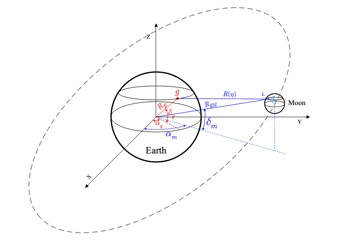
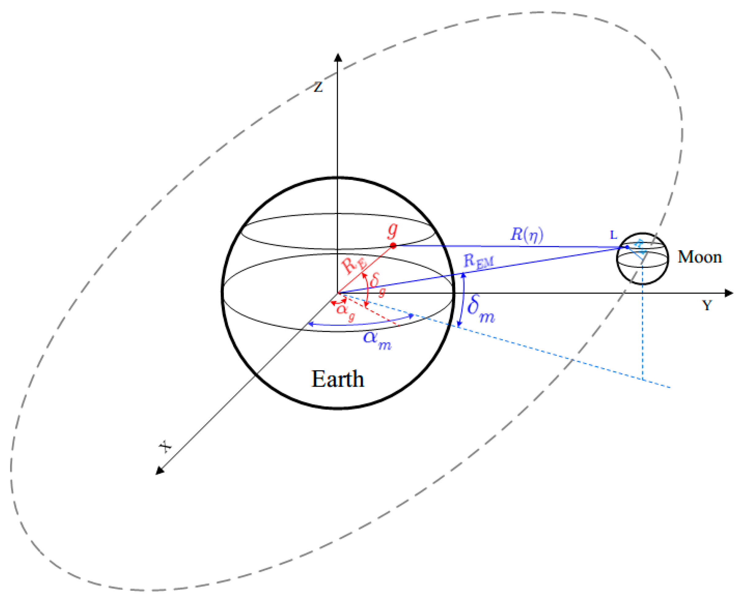
As the selection of the lunar base-station site is still under study [16], the exact coordinates of the Moon-Based SAR are undecided. Once the station site is selected, a right-handed geocentric inertial reference frame is defined, with the Z-axis towards the North Pole and the X-axis pointing to the true equinox of the date. The coordinate system is shown in Figure 1, where the lunar ascension and declination are designated by and the longitude and latitude of the ground target by . According to [17], when the ascending node of the lunar orbit points to the true equinox of the date, the lunar declination reaches its maximum value under this defined reference frame. Now that the Moon-Based SAR and the ground target are unified under the same coordinate system. The Doppler parameters are discussed in the following sections.
3. The Doppler Parameters of Moon-Based SAR
It is noted that the effect of the lunar revolution has been ignored for the simplicity in previous studies. On this basis, the Moon-Based SAR is assumed to be stationary and the synthetic aperture is realized simply by the rotation of the Earth [18]. However, the lunar revolution effect on the Doppler parameters is beyond negligible. To start with, the Doppler parameters for a stationary Moon-Based SAR are given for reference.
3.1. Doppler Parameters for a Stationary Moon-Based SAR
Without loss of generality, we initialize the time to zero when the distance between the ground target and the Moon-Based SAR is smallest. The slant range between SAR and ground target at time takes the expression
where the coefficients are explicitly given by
where are the coordinates of the motionless Moon-Based SAR system, with
Note that is the latitude at time ; the initial latitude at time zero; and, the Earth’s rotation angular velocity. Note that that the initial latitude was set to zero in the previous studies [9,12].
The 1st-order derivative of the slant range reads
According to [19], the Doppler frequency can be written as
where is the radar wavelength.
It follows that the Doppler centroid takes the form [8]
where is the beam center crossing time.
The exposure time is defined as [20]
where is the linear velocity of ground target, defined as , and is the aperture length of Moon-Based SAR in azimuthal direction.
The total Doppler bandwidth during the target exposure is obtained by [21]
The 2nd term in the above equation is generally much smaller than the 1st term by two or three orders of magnitude and can be neglected. Though the exposure time of the Moon-Based SAR is in the order of hundreds of seconds, is very small. Consequently,
Then, the Doppler bandwidth rate is approximated to
The azimuthal resolution is now given by
From above equation, it is seen that the azimuthal resolution is no longer just [8], but is now modified by three terms: , , and . That is, the azimuthal resolution is determined by the aperture length, the relative position of the ground target and SAR, and the Earth’s radius and the distance between the Earth and the SAR. In general, for a specific position of the Earth’s target and the SAR, the Earth’s radius and the distance between the Earth and the Moon-Based SAR can be assumed to be constant. The azimuthal resolution given in Equation (12) is illustrated using the simulation parameters in Table 1.
(1) Effect of declination of Moon-Based SAR.
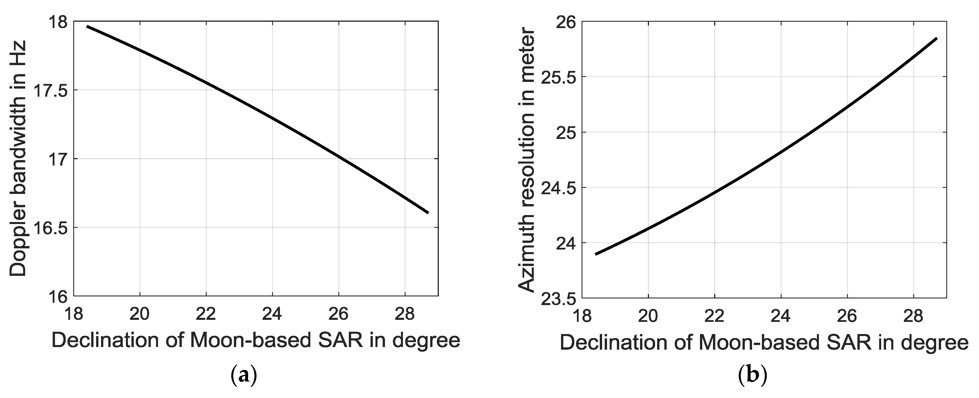
We investigate the impact of the declination of the Moon-Based SAR on the azimuthal resolution; the rest of the simulation parameters remain unchanged except for a variation in the declination of the lunar–based SAR. The Doppler bandwidth and azimuthal resolution are plotted as a function of the Moon-Based SAR’s declination in Figure 2a,b, respectively. In both cases, we set . As shown, when the declination increases, the Doppler bandwidth decreases, while the azimuthal resolution becomes coarser, as expected.
(2) Effects of ground target’s latitude.
From the exposure time given in Equation (9), with the latitude increases, the linear velocity of the Earth decreases, with a slight change in slant range. The net effect is an increased exposure time, which in turn affects the azimuthal resolution. To show this, we plot the exposure time and azimuthal resolution, as a function of the ground target’s latitude in Figure 3a,b by letting . From Figure 3, the azimuthal resolution becomes finer with the increasing of the ground target’s latitude. This is contributed by the reduction of the linear speed, leading to increasing exposure time.
(3) Effect of azimuthal visible range.
From Equation (12), a factor that is related to the azimuthal visible range, is confined by
where is the azimuthal visible range.
To be more explicitly, the factor in (13) is bounded in
As seen, the lower bound of Equation (13b) has a positive correlation with the azimuthal visible range as well as the absolute value of the ground target’s latitude, which indicates that with the increasing of the azimuthal visible range, the Doppler bandwidth increases, resulting in a finer azimuthal resolution.
As an example, the maximum of the azimuthal visible range is set to 6000 km for a ground target latitude of 22.5 degrees. The Doppler bandwidth and azimuthal resolution are plotted as a function of the azimuthal visible range in Figure 4.
As evident from Figure 4, when the azimuthal visible range is limited to less than 1000 km with target’s latitude of 22.5 degrees, the effect of the visible range is quite small. However, for a larger visible range, the Doppler bandwidth increases, resulting a finer azimuthal resolution. For an azimuthal visible range that is smaller than 1000 km, the factor is negligible; thus, the azimuthal resolution can be approximated to
Nevertheless, in general, the factor should be taken into account in determining the azimuthal resolution, as given in Equation (12).
3.2. Doppler Parameters for a Motional Moon-Based SAR
In the preceding sub-section, the Doppler parameters are evaluated by considering the Earth’s rotation only. However, because the Moon revolves around the Earth with an average rotational velocity of 1023 m/s, the Doppler parameters is much more involved when both rotation and revolution exerts. We need to consider the Moon revolution velocity, . The inclination between the plane of the Earth’s equator and the Moon revolution orbit is denoted by , which, typically, ranges from 18.3° to 28.6°, with a period of 18.6 years [22]. Since the variation of is extremely small during the exposure time, in what follows, the inclination is assumed a constant.
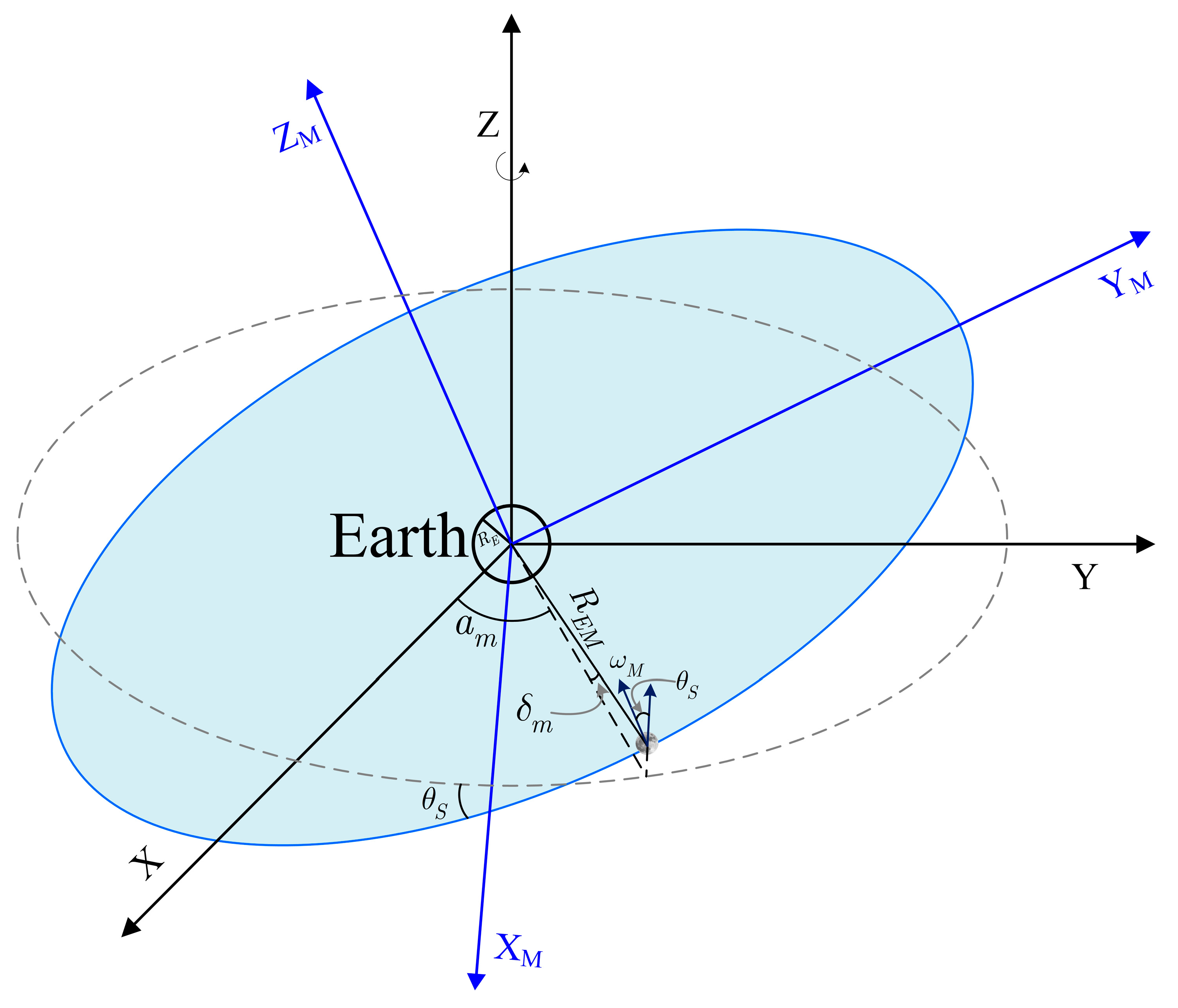
Figure 5 shows that the projected angle of the revolution velocity to the X-Y plane can be regarded as the inclination of that Moon-Based SAR, which varies to a limited extent during the exposure time. Consequently, the angular velocity of lunar revolution can be decomposed into two components along and perpendicular to the Z-axis as and , respectively. It is worth noting that as long as declination of Moon-Based SAR reaches the maximum value or minimum value, the sign of should change (+: for minimum to maximum; -: for maximum to minimum).
If the Moon shares the same orbit with the Earth’s self-rotation, the effect of the lunar revolution is quite limited, but non-negligible. However, a squint angle is caused by , resulting in a more complicated imaging geometry due to an inclination between the lunar orbit and the orbit of the Earth’s self-rotation. In addition, the presence of changes the position vector. When the Moon-Based SAR rotates around an angle of in X-Y plane from time 0 to time , rather than stationary, where , the slant vector of the motional Moon-Based SAR is totally different from that of the stationary Moon-Based SAR. Accordingly, it is of vital importance to consider the effect of the lunar revolution on the Moon-Based SAR imaging.
Now that the motional Moon-Based SAR’s ascension can be rewritten as , and its declination can be expressed as . As a result, the coordinates of the Moon-Based SAR can be expressed as
We can obtain the slant range in the context of the motional Moon-Based SAR:
The Doppler frequency of the Moon-Based SAR in considering the lunar revolution can be modified as
where is the Doppler frequency that is contributed by the Earth’s rotation:
is the contributed by the lunar revolution:
Noted that for , the Doppler frequency reduces to that of a stationary Moon-Based SAR in Equation (6).
The Doppler FM rate can be approximated by the equation
where is the part of the Doppler FM rate mainly contributed by the Earth’s rotation
and is the part of the Doppler FM rate that is mainly contributed by the lunar revolution
and is the coupling term of the Doppler FM rate between Earth’s rotation () and lunar revolution ():
For , Equation (19) reduces to Equation (7).
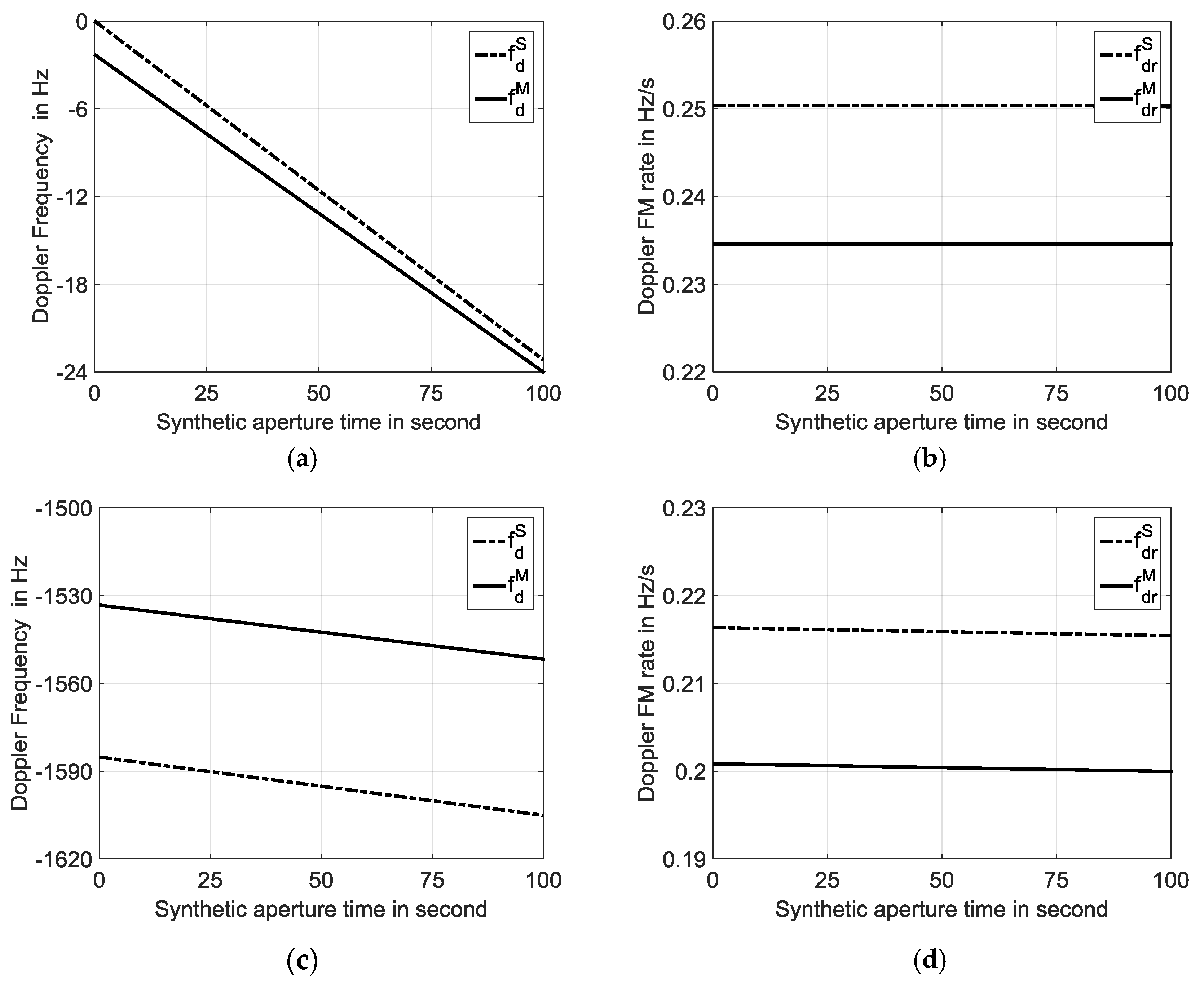
It is interested to compare the Doppler frequency and Doppler FM rate for stationary and motional Moon-Based SAR. For a numerical illustration, we use the parameters shown in Table 1 with two cases of visible ranges: and . From Figure 6, for a small visible range in azimuth, the motional Moon-Based SAR produces larger Doppler frequency, but not much, compared to the stationary one. The Doppler FM rate is little smaller in comparison, as seen from Figure 6b. For a large visible range in azimuth, the difference of Doppler frequency between the motional and the stationary Moon-Based SARs is now much larger, as shown in Figure 6c. Again, the Doppler FM rate is not changed much, as seen from Figure 6d.
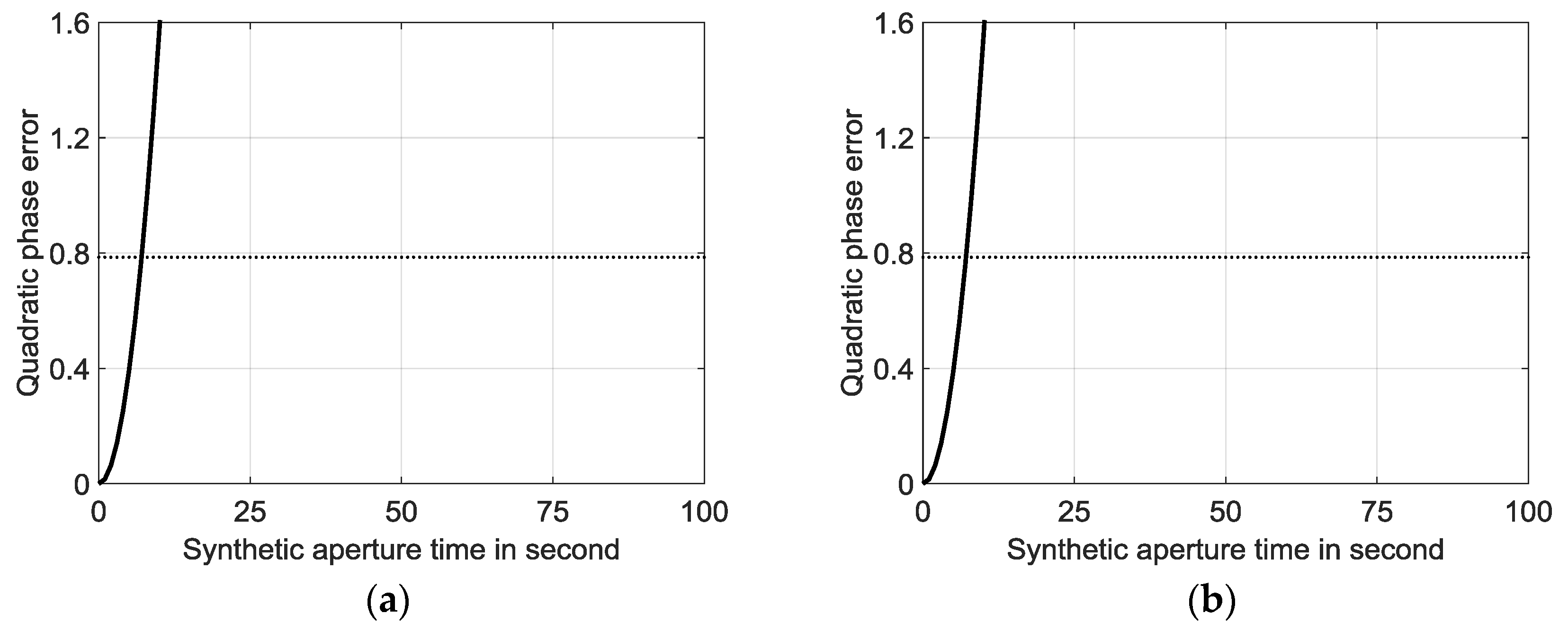
It is noted that the change of Doppler frequency leads to extra quadratic phase error [19], which affects the image focusing. To this end, in Figure 7a,b we plot the quadratic phase error that is caused by the lunar revolution, using the same parameters as in Figure 6b,d. From Figure 7, we see that quadratic phase error exceeds the threshold of . Thus, the imaging defocusing, mainly the image shift, is expected and should be corrected
The Doppler bandwidth is the product of the absolute value of the Doppler FM rate and the exposure time. It is instructive to compare the Doppler bandwidth between a motional Moon-Based SAR and a stationary Moon-Based SAR, and the corresponding azimuthal resolutions. The Doppler bandwidth and the azimuthal resolution with varying ground target latitudes, ranging from 0 to 80 degrees are shown in Figure 8a,b respectively, where the declination of the Moon-Based SAR is assumed 24.5 degrees. The Doppler bandwidth and azimuthal resolution as functions of the declination with a ground target located at (0, 0) are plotted in Figure 8c,d.
From Figure 8a,c we can observe that the Doppler bandwidth of a motional Moon-Based SAR is slightly different from that of a stationary Moon-Based SAR. The azimuthal resolutions of the motional Moon-Based SAR and of the stationary Moon-Based SAR are almost the same, as shown in Figure 8b,d, because both the velocity of strip and Doppler bandwidth decreases due to the lunar revolution.
At this point, the Doppler parameters of the motional Moon-Based SAR are discussed. It is found that the Doppler frequency and the Doppler FM rate of the motional Moon-Based SAR are different from those of the stationary Moon-Based SAR, indicating that the lunar-revolution must be considered. In the next section, the issue of signal propagation time delay for Moon-Based SAR is discussed.
3.3. Doppler Parameters for a Motional Moon-Based SAR
The motional Moon-Based SAR is disturbed by the error that is caused by the ‘stop-and-go’ assumption [23]. To be more complete, in the context of the total time delay, the earth’s rotation, and lunar revolution should be considered. The total time delay consists of two terms:
where is the arriving time of the transmitted signal to the ground target, which is given by
is the received time of a backscattered signal, which can be approximated by [24]
where is the slant range under lunar revolution; the speed of light.
The slant range of a motional Moon-Based SAR without assuming the ‘stop-and-go’ is given as
Under this condition, the Doppler frequency can be expressed as
where is given in Equation (18), and takes the same form as with .
The Doppler FM rate of a motional Moon-Based SAR without the ‘stop-and-go’ assumption can be approximated as
where is given in Equation (19).
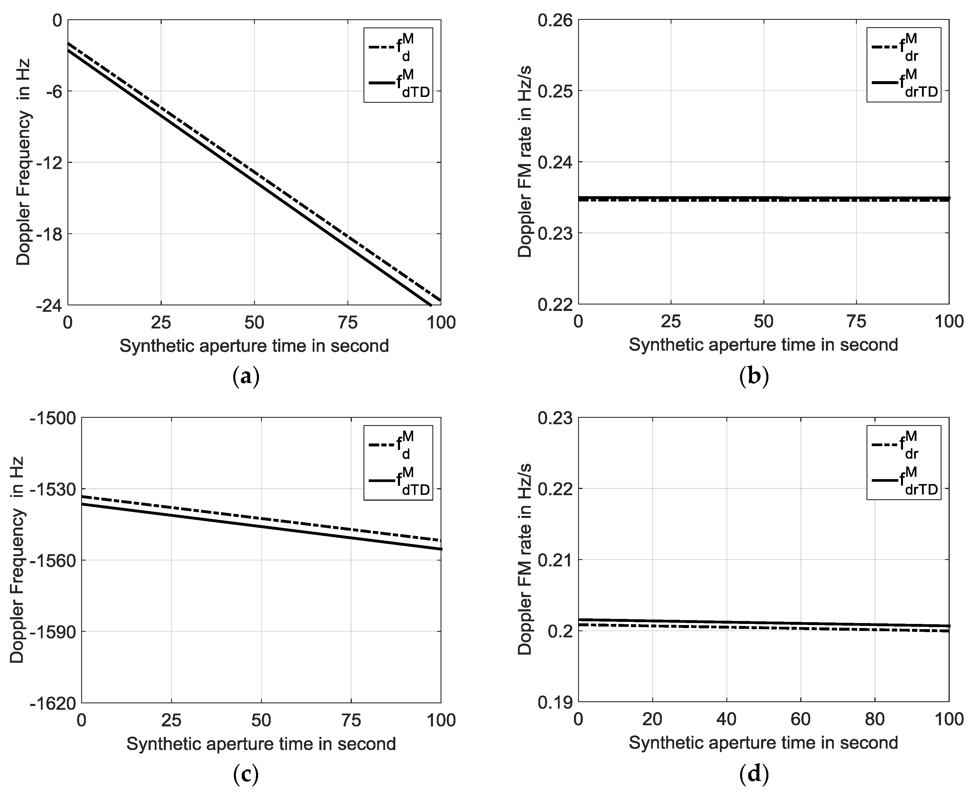
The Doppler parameters of a motional Moon-Based SAR without assuming stop-and-go becomes more complex, but more accurate. To illustrate this, in Figure 9, we plotted the Doppler frequency and the Doppler FM rate after removal of ‘stop-and-go’ assumption with the same simulation parameters, as in Figure 6. The error in the Doppler frequency and Doppler FM rate caused by the ‘stop-and-go’ assumption is relatively small for a smaller visible range in azimuth; is modified by it. With increase of the azimuth visible range, the error is large enough to cause image shift in azimuth direction. However, the variation of the Doppler FM rate is relatively small, as evident in Figure 9b,d, implying that the azimuthal resolution remains almost the same.
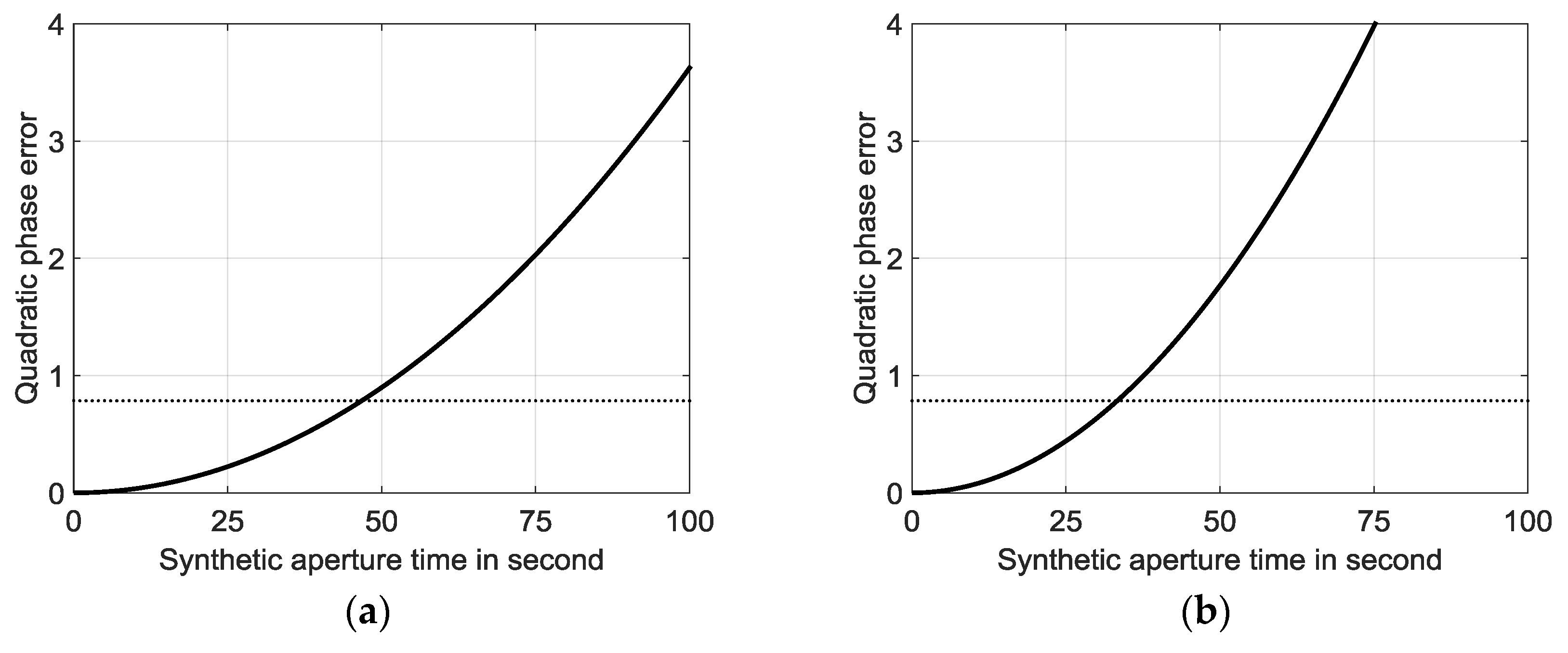
To further assess the influence of the change of Doppler FM rate on imaging focusing, we plot the quadratic phase error due to the total time delay in Figure 10a,b. As evident in Figure 10, the quadratic phase error exceeds its threshold of during an exposure time of 100 s. Consequently, in estimating the Doppler parameters, the error that is caused by the total time delay should be considered if image shift in azimuth is to be corrected.
The azimuthal resolution, with and without propagation time delay, as a function of the latitude of the ground target and declination are respectively plotted in Figure 11a,b, with the Moon-Based SAR placed (0, 28.5°). In Figure 11b, the target is located at (0, 0). From Figure 11a,b, it demonstrates that the azimuthal resolutions with and without the propagation time delay are almost the same, since the Doppler bandwidth and the exposure time are only slightly modified by the propagation time delay.
From above, The Doppler parameters can be affected by the lunar revolution and the ‘stop-and-go’ assumption, even though the azimuthal resolution is little impacted by both of them. On the other hand, the range resolution of the Moon-Based SAR, as in common SAR system, is given by
where is the system bandwidth.
In what follows, evaluation of the imaging properties of the Moon-Based SAR is presented.
4. Imaging Properties of Moon-Based SAR
In this section, we investigate the characteristics of Moon-Based SAR imaging. Before proceeding to the analysis, we need a signal model for the Moon-Based SAR based on the curve trajectory, where the relative positions of the Earth’s target and the Moon are accounted for.
4.1. Moon-Based SAR Signal Model
Before presenting the Moon-Based SAR signal model, we examine the relations between the exposure time of the Moon-Based SAR and the azimuthal resolution, by combining Equations (9) and (12), which is given:
Note that the term is due to the lunar revolution. We plot the exposure time of the Moon-Based SAR as a function of the azimuthal resolution in Figure 11. The simulation parameters remain the same as in Table 1, with .
Figure 12 shows that the exposure time of the Moon-Based SAR is in the order of hundreds of seconds, or even thousands of seconds. For a Moon-Based SAR, the large-scale phenomenon is of the most interest in observations, and thus it is preferable to design the azimuthal resolution on the decametric level.
Note that the straight path assumption that is used in traditional SAR imaging is no longer applicable in Moon-Based SAR imaging, but instead, a curve trajectory should be used. By expanding the slant range into a Taylor series about up to order, we have
where is the shortest slant range. The derivation of the expansion coefficients is tedious but straightforward. Appendix A lists these coefficients up to 3rd order.
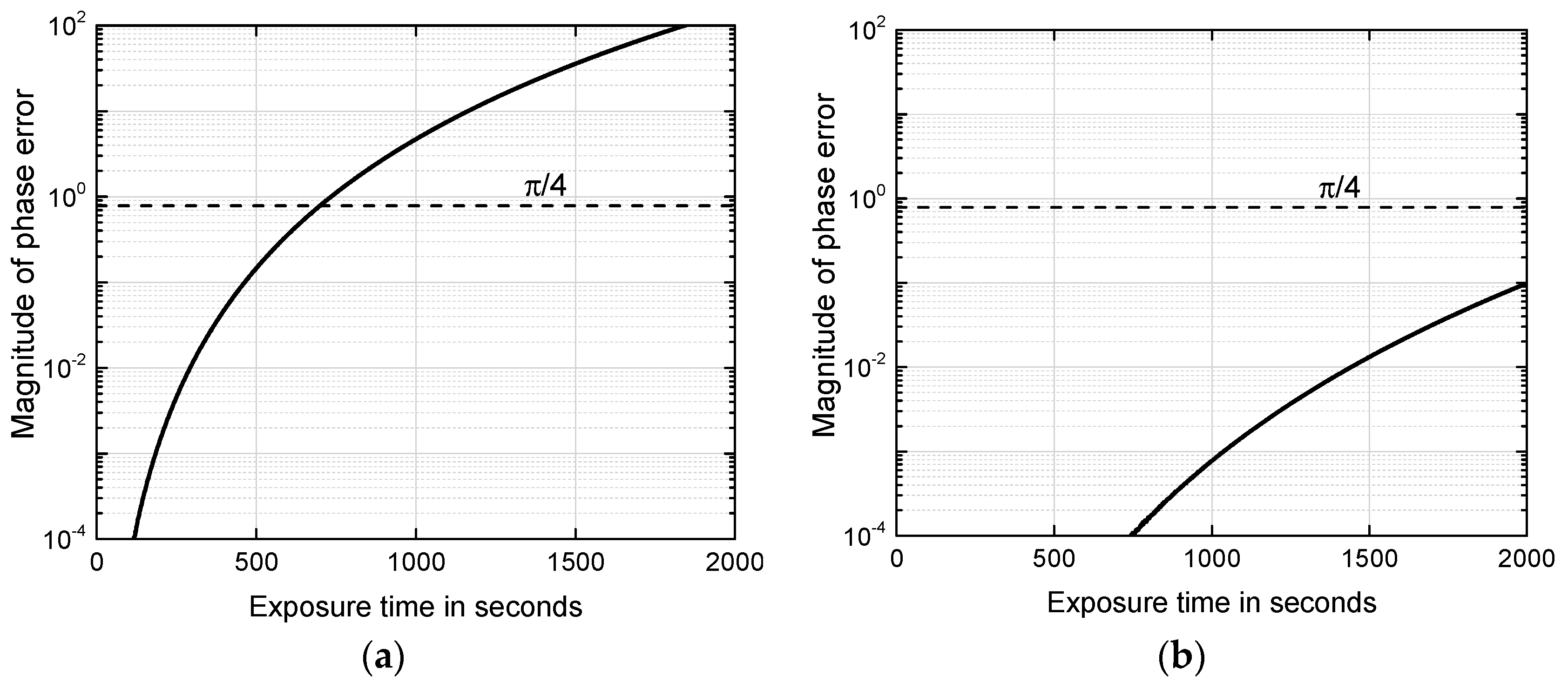
In Figure 13, plot the phase error as a function of exposure time, with parameters given in Table 1 and . It is clear that the 4th order curve trajectory is sufficient to meet the requirements of Moon-Based SAR imaging with an exposure time of 500 s and an azimuth visible range that is larger than 6000 km. However, when an azimuthal resolution in the range of meters is required, the corresponding exposure time ranges from 200 to 2000 s. For an exposure time longer than 700 s, the slant range expansion up to order is no longer enough, because the phase error exceeds the threshold of and an order expansion of the slant range is need to meet the metric level Moon-Based SAR imaging for a larger visible range.
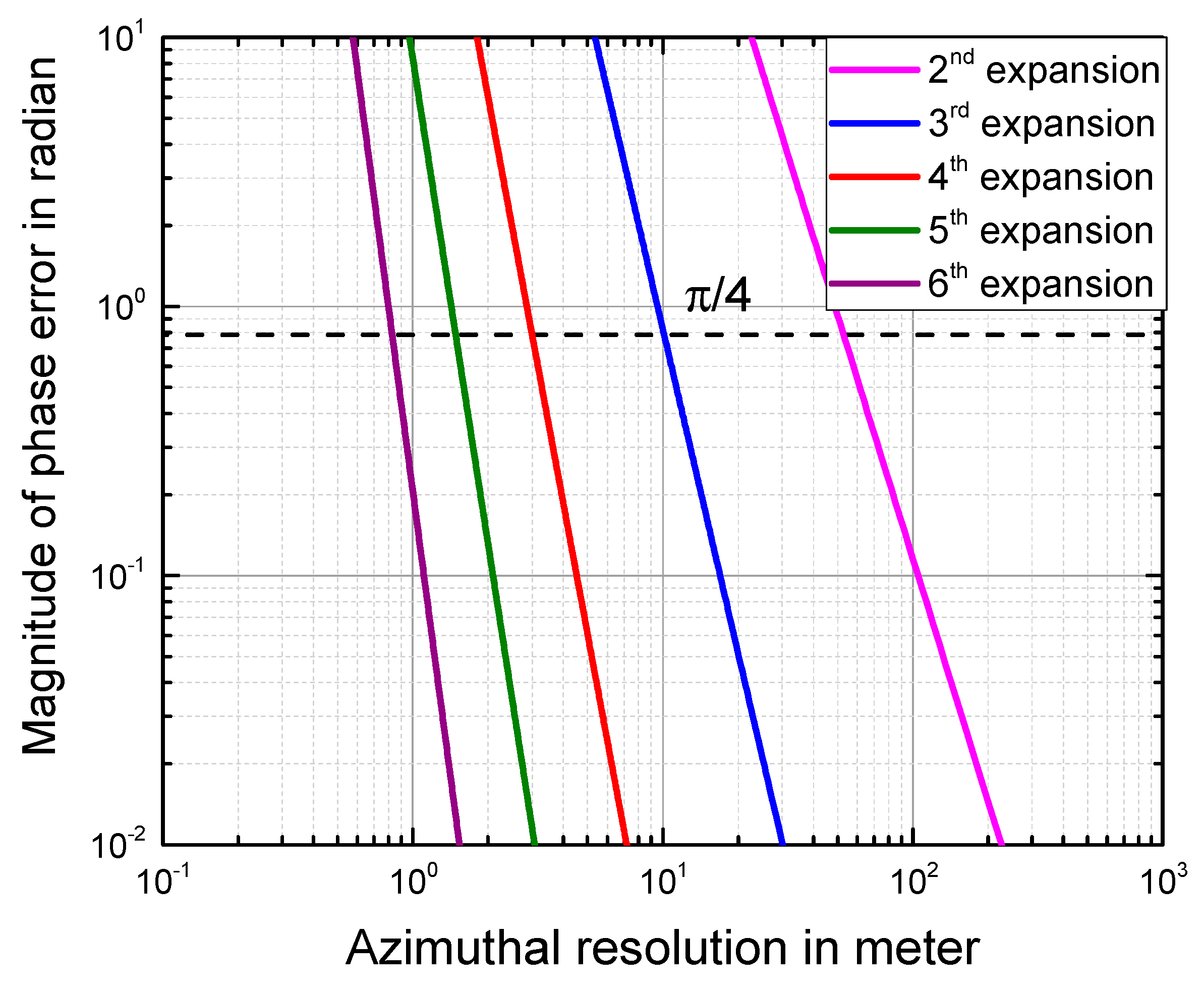
In Figure 14, we plot the azimuthal resolution dependence on the phase error in terms of the expansion orders. Within the phase threshold of , we see that the 6th-order expansion of the slant range is valid, even when an azimuthal resolution of 1 meter is required. In Table 2, we show the expansion orders and their corresponding azimuth resolution. An azimuthal resolution larger than 3.0 m can be achieved by a 4th order expansion curve trajectory. For a smaller azimuthal visible range, the azimuthal resolution becomes coarser within the valid expansion orders.
A Moon-Based SAR signal model with a 4th-order expansion curve trajectory is adopted in the following analysis. The received signal of the Moon-Based SAR from a single point target can be expressed as [19]
where and are window functions in the fast time and slow time domains, respectively. is the chirp rate, and is the carrier frequency.
The two-dimensional (2-D) signal spectrum of Equation (28) can be obtained by using the method of series reversion (MSR) [25] and the principle of stationary phase (POSP) [26],
where the phase spectrum takes the form
where , , , , . From the above Equation (28.a), the range and azimuth frequency are highly coupled in the phase term . Detailed derivation is given in Appendix B.
To process the signal of the Moon-Based SAR, Equation (28.a) is further expanded as
where is in connection with the azimuth compression, and its specific expression is given by
is related to the range compression, which can be written as
is related to the secondary range compression given by
concerns the range cell migration and takes the form:
Finally, is the residual phase term that has a bearing on the polarization:
At this point, the signal model and 2-D spectrum based on the curve trajectory are derived, and the Moon-Based SAR can be achieved by using the Range Doppler algorithm [27]. The characteristics of Moon-Based SAR imaging are studied in the next sub-section.
4.2. Properties of Moon-Based SAR Imaging
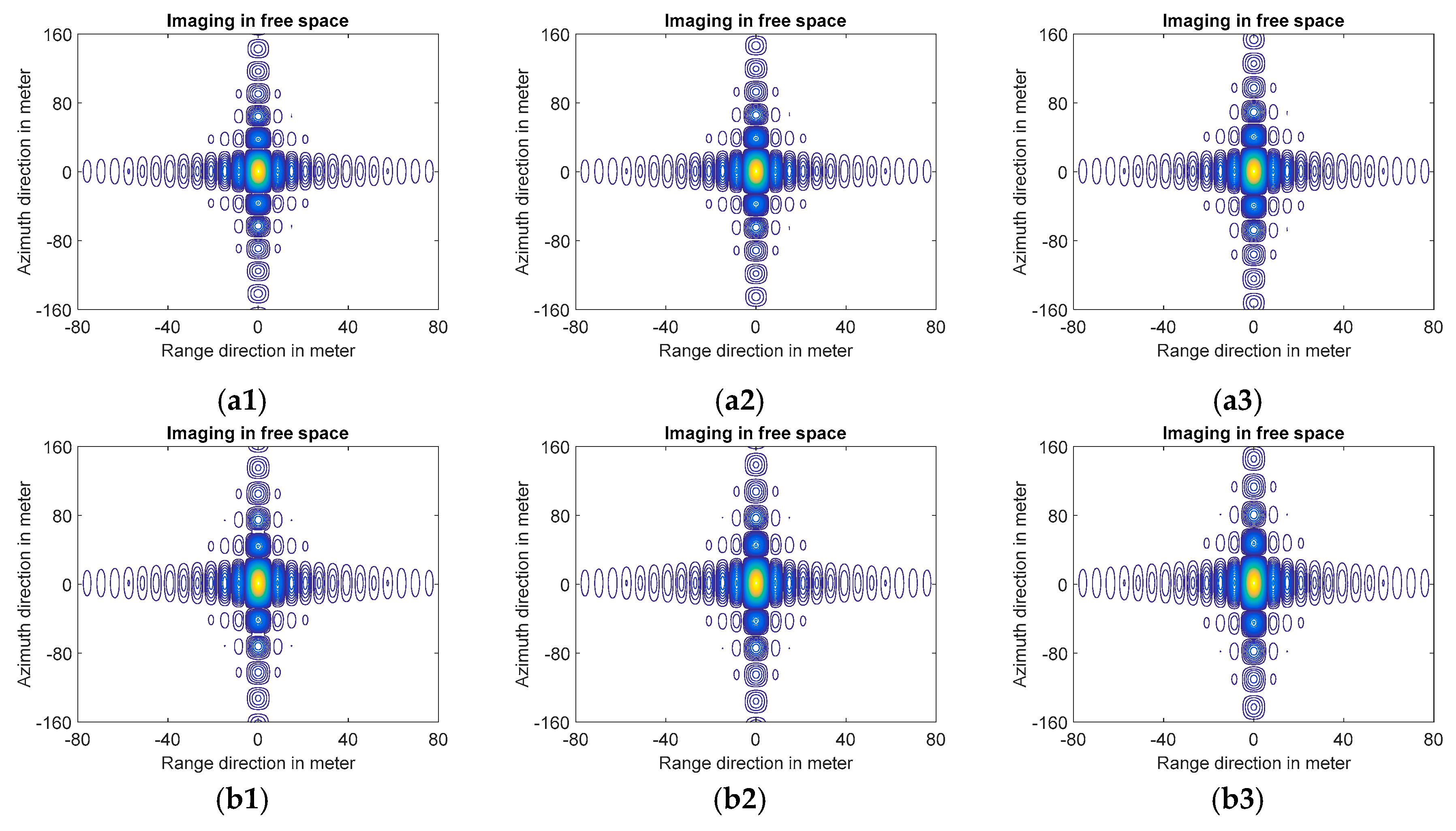
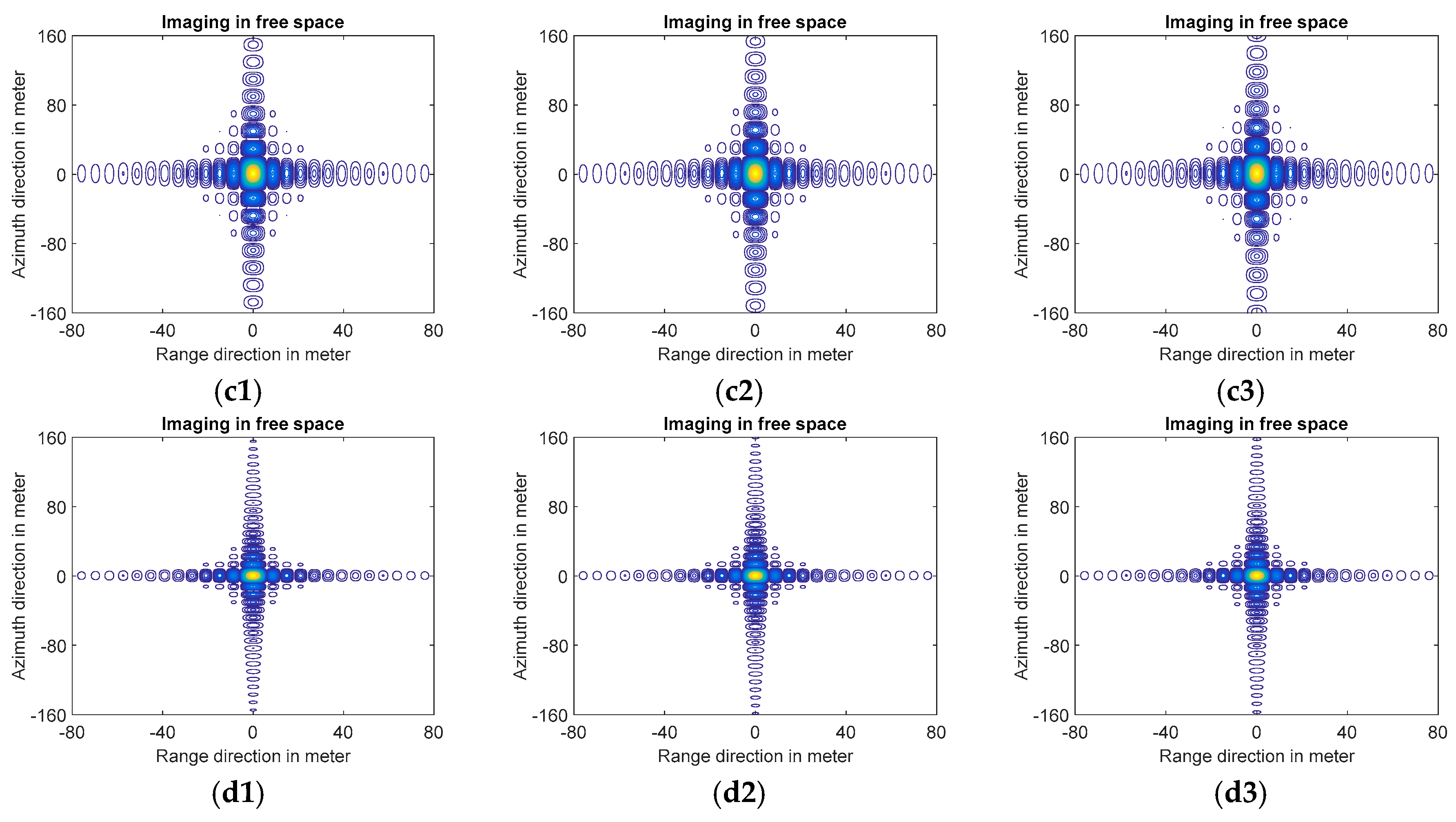
From Equation (14), the azimuthal resolution is a function of the ground target’s position, the Moon-Based SAR’s position and the aperture length in the azimuth. We plot the point target image in azimuth and range directions in Figure 15, for three declination angles: 18 degrees, 22 degrees, and 28 degrees, respectively, shown in 1st (a1,b1,c1,d1), 2nd (a2,b2,c2,d2), and 3rd (a3,b3,c3,d3) columns. As we can see from Figure 15, the latitude of the ground target is the most crucial factor in determining the azimuthal imaging of Moon-Based SAR. The quantitative values of azimuthal resolutions are listed in Table 3.
5. Conclusions
The signal model for Moon-Based SAR imaging is investigated using a complex, but more complete, geometry of Moon-Based SAR and Earth, where the rotations and revolutions are considered. A unified right-handed geocentric inertial reference coordinate system for the Moon-Based SAR is established, followed by analyzing the Doppler parameters under different conditions. It is found that the lunar revolution and the error that is caused by the ‘stop-and-go’ assumption are potentially significant to affect the Doppler parameters, and thus must be taken into account in the image focusing. The Doppler bandwidth and exposure time, on the other hand, are much less affected, and as a result the azimuthal resolution remains almost unaffected. The signal model and its 2-D spectrum of a motional moon-based SAR without imposing the ‘stop-and-go’ assumption are derived. The expansion orders considering azimuthal resolutions are analyzed.
Acknowledgments
This work was supported by National Natural Science Foundation of China under the grants 41580853 and 41531175, and the Director General’s Innovative Funding-2015.
Author Contributions
Kun-Shan Chen and Zhen Xu conceived and developed the theory and signal model; Zhen Xu performed the numerical simulations; Zhen Xu and Kun-Shan Chen wrote the paper.
Conflicts of Interest
The authors declare no conflict of interest.
Appendix A
The derivation of the expansion coefficients appearing in Equation (26) is tedious but straightforward. For reference and for saving space, coefficients up to 3rd order are given below.
Appendix B
The slant distance, considering the lunar revolution and without assuming the “stop and go”, is expanded about the slow time up to order:
To apply MSR, the linear phase term of the received signal need to be removed:
where
The Fourier transform in range direction is applied to Equation (A6) by using principle of stationary phase method:
Next, the Fourier transform is carried out in azimuth direction:
The phase term in the above Fourier integral is
Taking the derivative of with respect to , we have
By way of POSP, we obtain
The slow time can be expressed in terms of via MSR
where the coefficients are , , .
Substituting the slow time (A12) into (A9), we arrive at the two-dimensional (2D) frequency spectrum of Equation (A6):
where the exponent is given by
According to the skew and shift properties of the Fourier transform, is substituted by in Equation (A13) and the corresponding 2-D spectrum is given as
Keeping up to order, the phase term can be written as and the phase can be written as
The range and azimuth frequencies are highly coupled in the phase term. To proceed, Equation (A15) is further expanded as follows:
where
References
- Campbell, J.B.; Wynne, R.H. Introduction to Remote Sensing; Guilford Press: New York, NY, USA, 2011. [Google Scholar]
- Johnson, J.; Lucey, P.; Stone, T.; Staid, M. Visible/Near-Infrared Remote Sensing of Earth from the Moon. NASA Advisory Council Workshop on Science Associated with the Lunar Exploration Architecture White Papers; 2007. Available online: http://www.lpi.usra.edu/meetings/LEA/whitepapers/Johnson_etal_v02.pdf (accessed on 19 July 2017).
- Renga, A. Configurations and Performance of Moon-based SAR Systems for very high resolution Earth remote sensing. In Proceedings of the AIAA Pegasus Aerospace Conference, Naples, Italy, 12–13 April 2007. [Google Scholar]
- Renga, A.; Moccia, A. Preliminary analysis of a Moon-based Interferometric SAR system for very high resolution Earth remote sensing. In Proceedings of the 9th ILEWG International Conference on Exploration and Utilisation of the Moon, Sorrento, Italy, 22–26 October 2007. [Google Scholar]
- Moccia, A.; Renga, A. Synthetic aperture radar for earth observation from a lunar base: Performance and potential applications. IEEE Trans. Aerosp. Electron. Syst. 2010, 46, 1034–1051. [Google Scholar] [CrossRef]
- Fornaro, G.; Franceschetti, G.; Lombardini, F.; Mori, A.; Calamia, M. Potentials and limitations of moon-borne sar imaging. IEEE Trans. Geosci. Remote Sens. 2010, 48, 3009–3019. [Google Scholar] [CrossRef]
- Purkis, S.J.; Klemas, V.V. Remote Sensing and Global Environmental Change; John Wiley & Sons: Chichester, West Sussex, UK, 2011. [Google Scholar]
- Chen, K.-S. Principles of Synthetic Aperture Radar Imaging: A System Simulation Approach; CRC Press: Boca Raton, FL, USA, 2016. [Google Scholar]
- Guo, H.D.; Ding, Y.X.; Liu, G.; Zhang, D.W.; FU, W.X.; Zhang, L. Conceptual study of lunar-based sar for global change monitoring. Sci. China Earth Sci. 2014, 57, 1771–1779. [Google Scholar] [CrossRef]
- Ding, Y. Moonborne Earth Observation Synthetic Aperture Radar and Its Application in Global Change. Ph.D. Thesis, Signal and Information Processing, University of Chinese Academy of Sciences, Beijing, China, 2014. [Google Scholar]
- Ren, Y.; Guo, H.; Liu, G.; Ye, H. Simulation study of geometric characteristics and coverage for moon-based earth observation in the electro-optical region. IEEE J. Sel. Top. Appl. Earth Obs. Remote Sens. 2017, 10, 2431–2440. [Google Scholar] [CrossRef]
- Guo, H.D.; Liu, G.; Ding, Y.X. Moon-based earth observation: Scientific concept and potential applications. Int. J. Digit. Earth 2017, 1–12. [Google Scholar] [CrossRef]
- Ouyang, Z.Y. Introduction to Lunar Science; China Astron Publ House: Beijing, China, 2005. [Google Scholar]
- Standish, E. Jpl Planetary and Lunar Ephemerides: De 405/le 405, Jet Propulsion Laboratory Interoffice Memorandum, IOM 312. F-98-048. August 1998. Available online: http://iau-comm4.jpl.nasa.gov/de405iom/de405iom.pdf (accessed on 23 September 2017).
- Meeus, J. Explanatory supplement to the astronomical ephemeris. Ciel et Terre 1962, 78, 376. [Google Scholar]
- Jia, Y.Z.; Zhou, Y.L. Research on lunar site selection for lunar based earth observation. Spacecr. Eng. 2016, 25, 116–121. [Google Scholar]
- Goldreich, P. History of the lunar orbit. Rev. Geophys. 1966, 4, 411–439. [Google Scholar] [CrossRef]
- Renga, A.; Moccia, A. Moon-based synthetic aperture radar: Review and challenges. In Proceedings of the IEEE International Geoscience and Remote Sensing Symposium, Beijing, China, 10–15 July 2016; pp. 3708–3711. [Google Scholar]
- Cumming, I.G.; Wong, F.H. Digital Signal Processing of Synthetic Aperture Radar Data: Algorithms and Implementation; Artech House: Boston, MA, USA, 2004. [Google Scholar]
- Skolnik, M. Radar Handbook, 2nd ed.; McGraaw-Hill Book Company: New York, NY, USA, 1990. [Google Scholar]
- Ulaby, F.T.; Long, D.G.; Blackwell, W.J.; Elachi, C.; Fung, A.K.; Ruf, C.; Sarabandi, K.; Zebker, H.A.; Van Zyl, J. Microwave Radar and Radiometric Remote Sensing; University of Michigan Press: Ann Arbor, MI, USA, 2014. [Google Scholar]
- Xi, X.N.; Zeng, G.Q.; Ren, X. Orbit Design of Lunar Probe; National Defence Industry Press: Changsha, China, 2001. [Google Scholar]
- Curlander, J.C.; Mcdonough, R.N. Synthetic Aperture Radar: Systems and Signal Processing; John Wiley & Sons: New York, NY, USA, 1991. [Google Scholar]
- Hu, C.; Long, T.; Zeng, T.; Liu, F.; Liu, Z. The accurate focusing and resolution analysis method in geosynchronous sar. IEEE Trans. Geosci. Remote Sens. 2011, 49, 3548–3563. [Google Scholar] [CrossRef]
- Neo, Y.L.; Wong, F.; Cumming, I.G. A two-dimensional spectrum for bistatic SAR processing using series reversion. IEEE Geosci. Remote Sens. Lett. 2007, 4, 93–96. [Google Scholar] [CrossRef]
- Key, E.L.; Fowle, E.N.; Haggarty, R.D. A method of designing signals of large time-bandwidth product. IRE Int. Conv. Rec. 1961, 4, 146–155. [Google Scholar]
- Wu, C.; Liu, K.Y.; Jin, M. Modeling and a correlation algorithm for spaceborne SAR signals. IEEE Trans. Aerosp. Electron. Syst. 1982, AES-18, 563–575. [Google Scholar] [CrossRef]
- Ishimaru, A.; Kuga, Y.; Liu, J.; Kim, Y.; Freeman, T. Ionospheric effects on SAR at 100 MHz to 2 GHz. Radio Sci. 1999, 34, 257–268. [Google Scholar] [CrossRef]
- Xu, Z.; Wu, J.; Wu, Z. A survey of ionospheric effects on space-based radar. Waves Random Media 2004, 14, S189–S273. [Google Scholar] [CrossRef]
- Quegan, S.; Lamont, J. Ionospheric and tropospheric effects on synthetic aperture radar performance. Int. J. Remote Sens. 1986, 7, 525–539. [Google Scholar] [CrossRef]
Figure 1.
An unified right-handed geocentric inertial reference coordinate system for Moon-Based synthetic aperture radar (SAR), where point g represents the ground target, REM is the distance between the Earth and the Moon-Based SAR, which can be approximately regarded as the Earth and the Moon, and RE is the earth radius at point g. (not to scale for the sake of clarity).

Figure 2.
(a) Relationship between Doppler bandwidth and Moon-Based SAR’s declination; (b) Azimuth resolution as a function of the Moon-Based SAR’s declination.
Figure 2.
(a) Relationship between Doppler bandwidth and Moon-Based SAR’s declination; (b) Azimuth resolution as a function of the Moon-Based SAR’s declination.

Figure 3.
Variations of the (a) Exposure time and (b) Azimuthal resolution. The ascension is set to zero degree.
Figure 3.
Variations of the (a) Exposure time and (b) Azimuthal resolution. The ascension is set to zero degree.
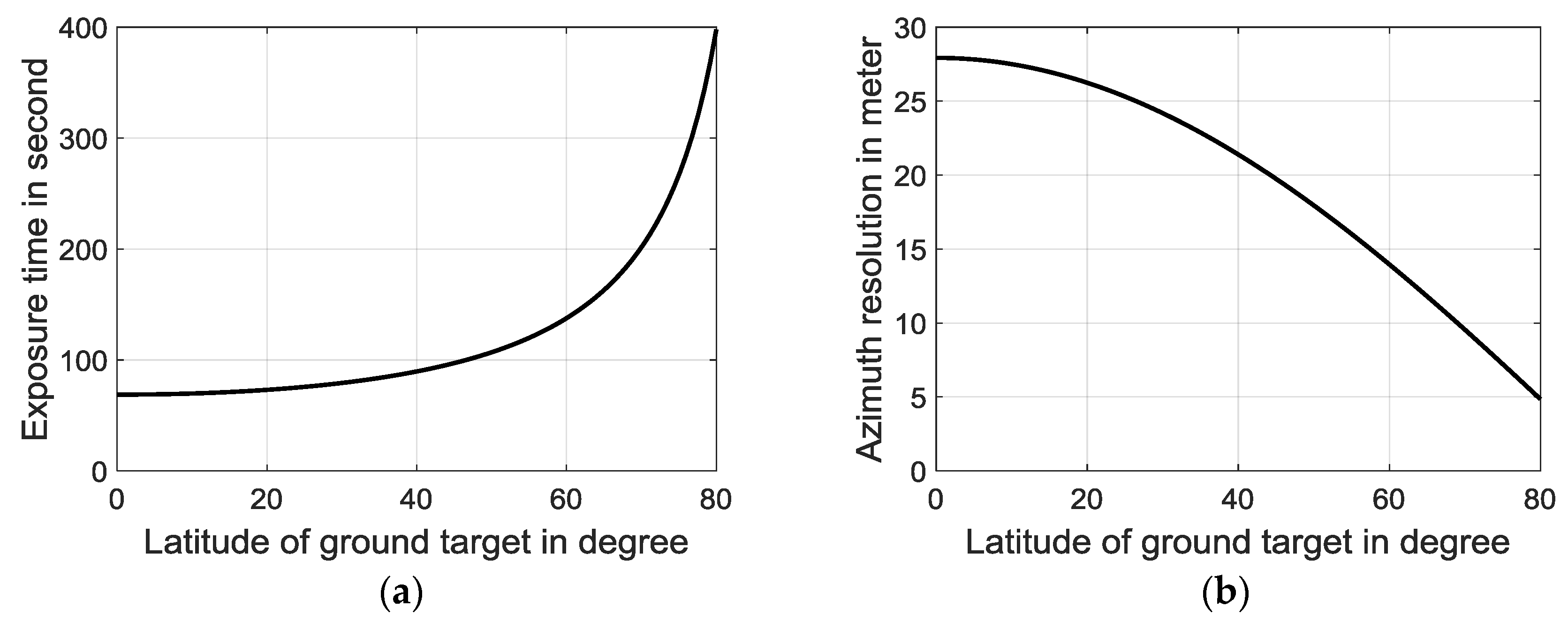
Figure 4.
Doppler bandwidth (a) and Azimuthal resolution (b) as a function of azimuth visible range.
Figure 4.
Doppler bandwidth (a) and Azimuthal resolution (b) as a function of azimuth visible range.
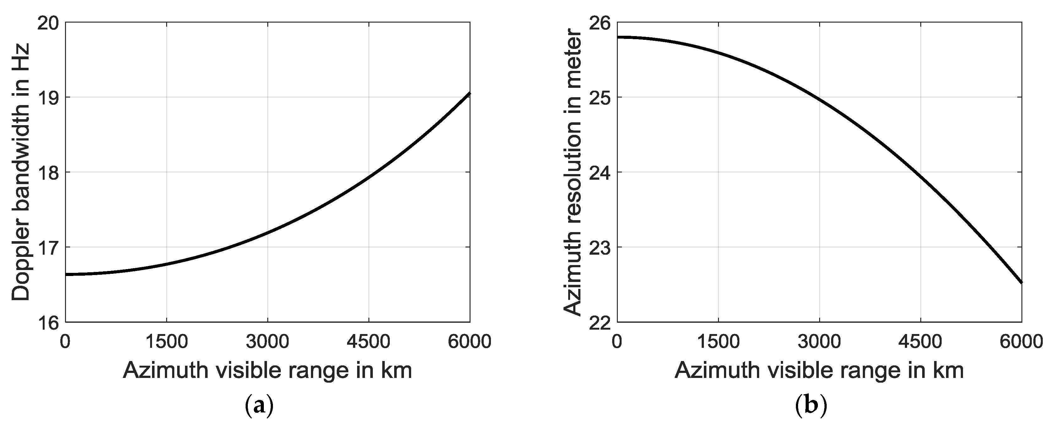
Figure 5.
Imaging geometry of Moon-Based SAR in consideration of lunar revolution.

Figure 6.
Comparison between the Doppler parameters of stationary Moon-Based SAR (superscript S) and motional Moon-Based SAR (superscript M) with a small visible range in azimuth and : (a) Doppler frequency; (b) Doppler frequency modulation (FM) rate; with a large visible range in azimuth ; (c) Doppler frequency; (d) Doppler FM rate.

Figure 7.
Quadratic phase error caused by the lunar revolution within an exposure time of 100 s: (a) (b) .
Figure 7.
Quadratic phase error caused by the lunar revolution within an exposure time of 100 s: (a) (b) .

Figure 8.
With the increasing ground target latitude, variations of the (a) Doppler bandwidth and (b) Azimuth resolution. With the increasing declination of the lunar-based SAR, the variations of the (c) Doppler bandwidth and (d) Azimuth resolution. The superscript S indicates the stationary Moon-Based SAR, while superscript M represents the motional Moon-Based SAR.
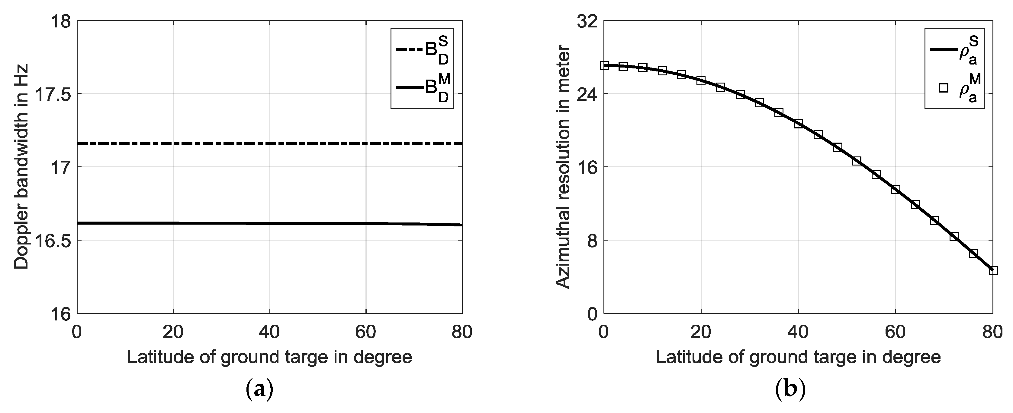
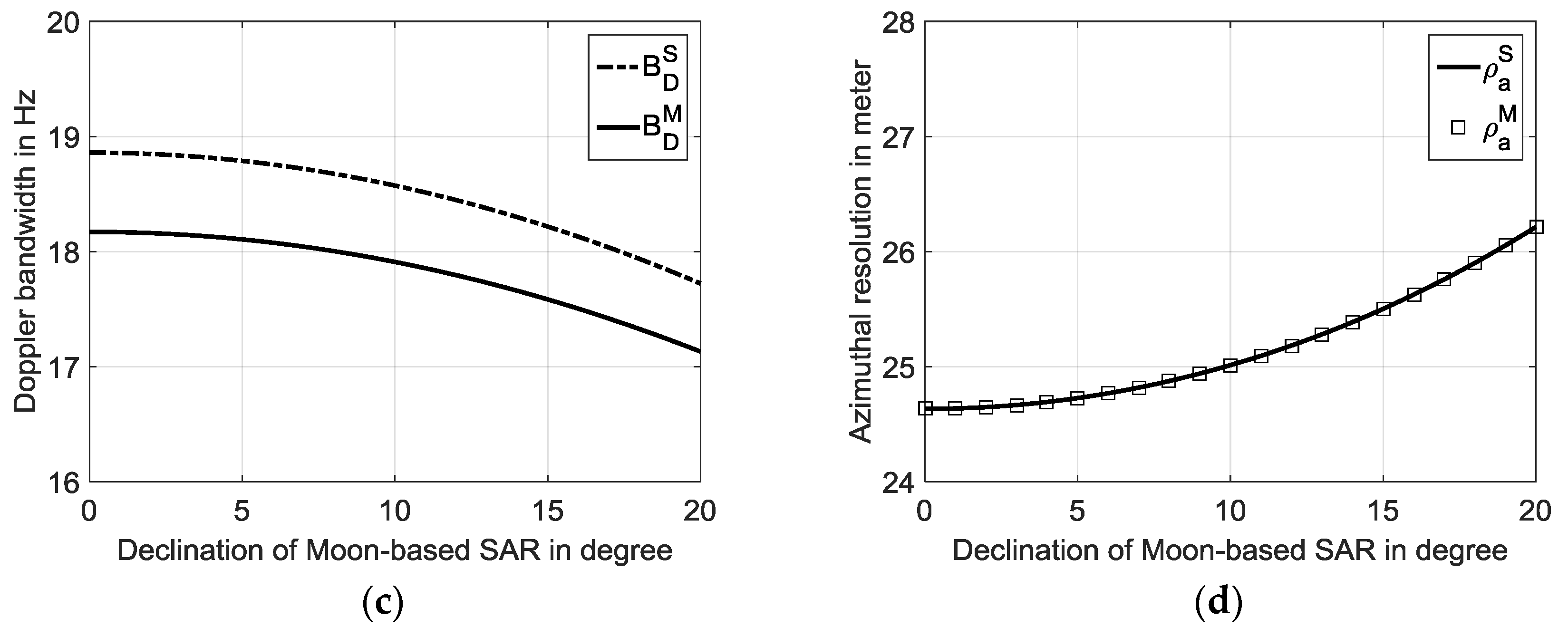
Figure 9.
Comparison between the motional Moon-Based SAR with the ‘stop-and-go’ assumption and that without the ‘stop-and-go’ assumption; equals 0: (a) Doppler frequency; (b) Doppler FM rate; with equal to ; (c) Doppler frequency; (d) Doppler FM rate.
Figure 9.
Comparison between the motional Moon-Based SAR with the ‘stop-and-go’ assumption and that without the ‘stop-and-go’ assumption; equals 0: (a) Doppler frequency; (b) Doppler FM rate; with equal to ; (c) Doppler frequency; (d) Doppler FM rate.

Figure 10.
Quadratic phase error caused by the total time delay during an exposure time of 100 s with: (a) (b) .
Figure 10.
Quadratic phase error caused by the total time delay during an exposure time of 100 s with: (a) (b) .

Figure 11.
Dependence of azimuthal resolution on (a) ground target latitude; (b) declination of the lunar-based SAR. Superscript M denotes motional Moon-Based SAR, and the additional superscript TD indicates the propagation time delay.
Figure 11.
Dependence of azimuthal resolution on (a) ground target latitude; (b) declination of the lunar-based SAR. Superscript M denotes motional Moon-Based SAR, and the additional superscript TD indicates the propagation time delay.
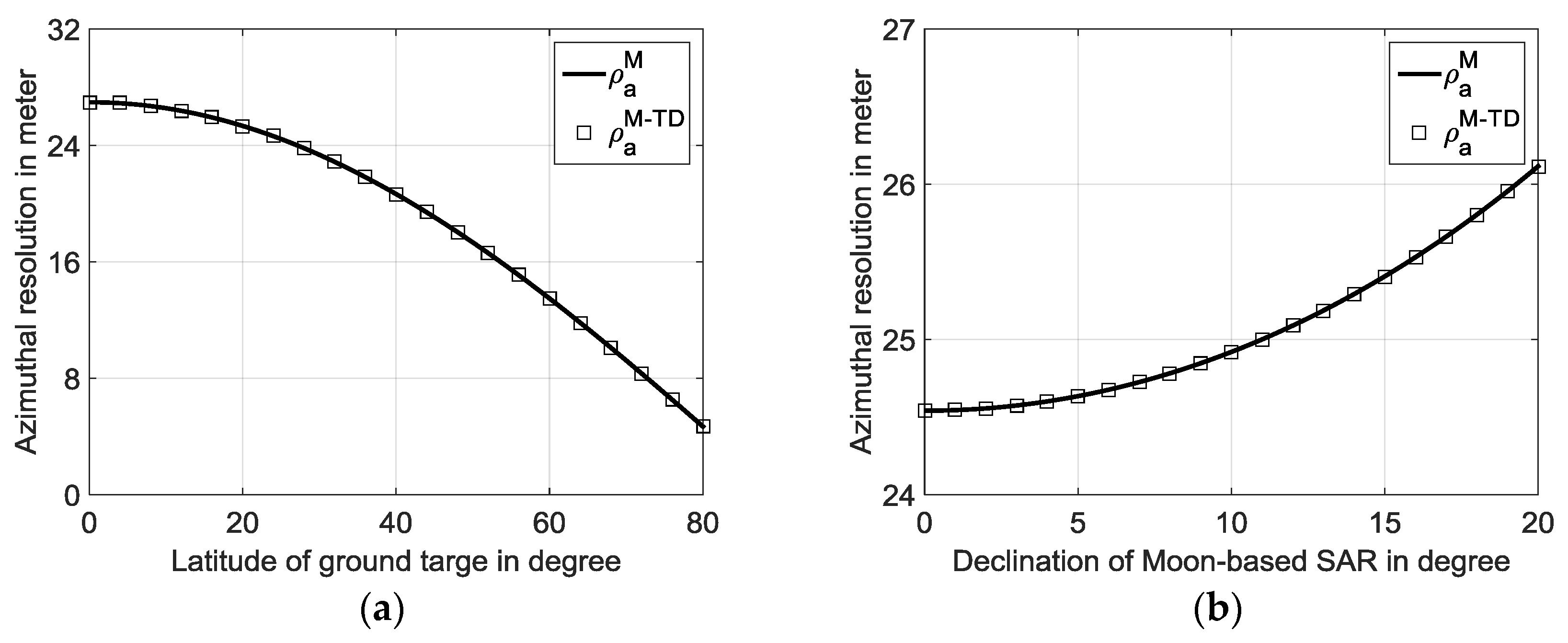
Figure 12.
Relationship between the exposure time and azimuthal resolution. Here, the declination of the moon is set to 28.5 degrees.
Figure 12.
Relationship between the exposure time and azimuthal resolution. Here, the declination of the moon is set to 28.5 degrees.
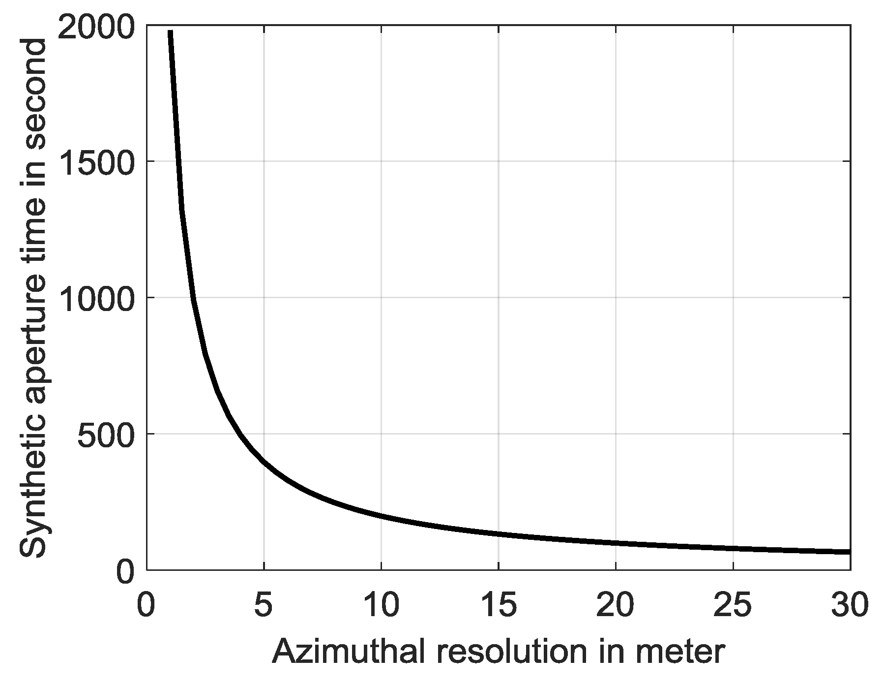
Figure 13.
Phase error with range expansion up to (a) 4th order and (b) 6th order.

Figure 14.
Relationship between the azimuthal resolution and phase error caused by different expansion orders.
Figure 14.
Relationship between the azimuthal resolution and phase error caused by different expansion orders.

Figure 15.
Comparison of azimuthal imaging with different positions, where the 1st (a1,b1,c1,d1), 2nd (a2,b2,c2,d2), and 3rd (a3,b3,c3,d3) columns show declination angle of 18 degrees, 22 degrees, and 28 degrees, respectively. The first row signifies a latitude of 0 degrees, with no difference between the ascension and longitude. The second row denotes a latitude of 0 degrees, with a difference of 30 degrees between the ascension and longitude. The 3rd row and 4th row show the case of latitude of 40 degrees and 70 degrees, respectively, both with no difference between ascension and longitude.


Table 1.
Simulation parameters.
| Parameter | Symbol | Quantity | Unit |
|---|---|---|---|
| Latitude of ground target | 22.5 | degree | |
| Declination of Moon-Based SAR | 24.5 | degree | |
| Inclination of lunar orbit to the equator of the Earth | 28.6 | degree | |
| Earth radius | 6371 | km | |
| Distance between the Earth and the Moon-Based SAR | 389,408 | km | |
| Earth’s rotation angular velocity | 7.292 × 10⁻⁵ | rad/s | |
| Lunar revolution angular velocity | 2.662 × 10⁻⁶ | rad/s | |
| Carrier frequency | 1.2 | GHz | |
| System bandwidth | 50 | MHz |
Table 2.
Relationship between azimuthal resolution and valid expansion orders.
| Expansion Order | Azimuthal Resolution | Unit |
|---|---|---|
| 2 | >52.9 | m |
| 3 | >10.2 | m |
| 4 | >3.0 | m |
| 5 | >1.5 | m |
| 6 | >0.85 | m |
Table 3.
Azimuthal Resolution of Simulation Results.
| Declination of Moon-Based SAR | () | () | () | |
| Latitude of Ground Target | ||||
| () | 25.8 m | 26.5 m | 27.8 m | |
| () | 29.8 m | 30.6 m | 32.1 m | |
| () | 19.8 m | 20.3 m | 21.3 m | |
| () | 8.8 m | 9.1 m | 9.5 m | |
© 2018 by the authors. Licensee MDPI, Basel, Switzerland. This article is an open access article distributed under the terms and conditions of the Creative Commons Attribution (CC BY) license (http://creativecommons.org/licenses/by/4.0/).
Share and Cite
MDPI and ACS Style
Xu, Z.; Chen, K.-S. On Signal Modeling of Moon-Based Synthetic Aperture Radar (SAR) Imaging of Earth. Remote Sens. 2018, 10, 486. https://doi.org/10.3390/rs10030486
AMA Style
Xu Z, Chen K-S. On Signal Modeling of Moon-Based Synthetic Aperture Radar (SAR) Imaging of Earth. Remote Sensing. 2018; 10(3):486. https://doi.org/10.3390/rs10030486
Chicago/Turabian StyleXu, Zhen, and Kun-Shan Chen. 2018. "On Signal Modeling of Moon-Based Synthetic Aperture Radar (SAR) Imaging of Earth" Remote Sensing 10, no. 3: 486. https://doi.org/10.3390/rs10030486
Note that from the first issue of 2016, this journal uses article numbers instead of page numbers. See further details here.