Evaluating Landsat and RapidEye Data for Winter Wheat Mapping and Area Estimation in Punjab, Pakistan

 ,
,
Abstract
:
1. Introduction
2. Materials and Methods
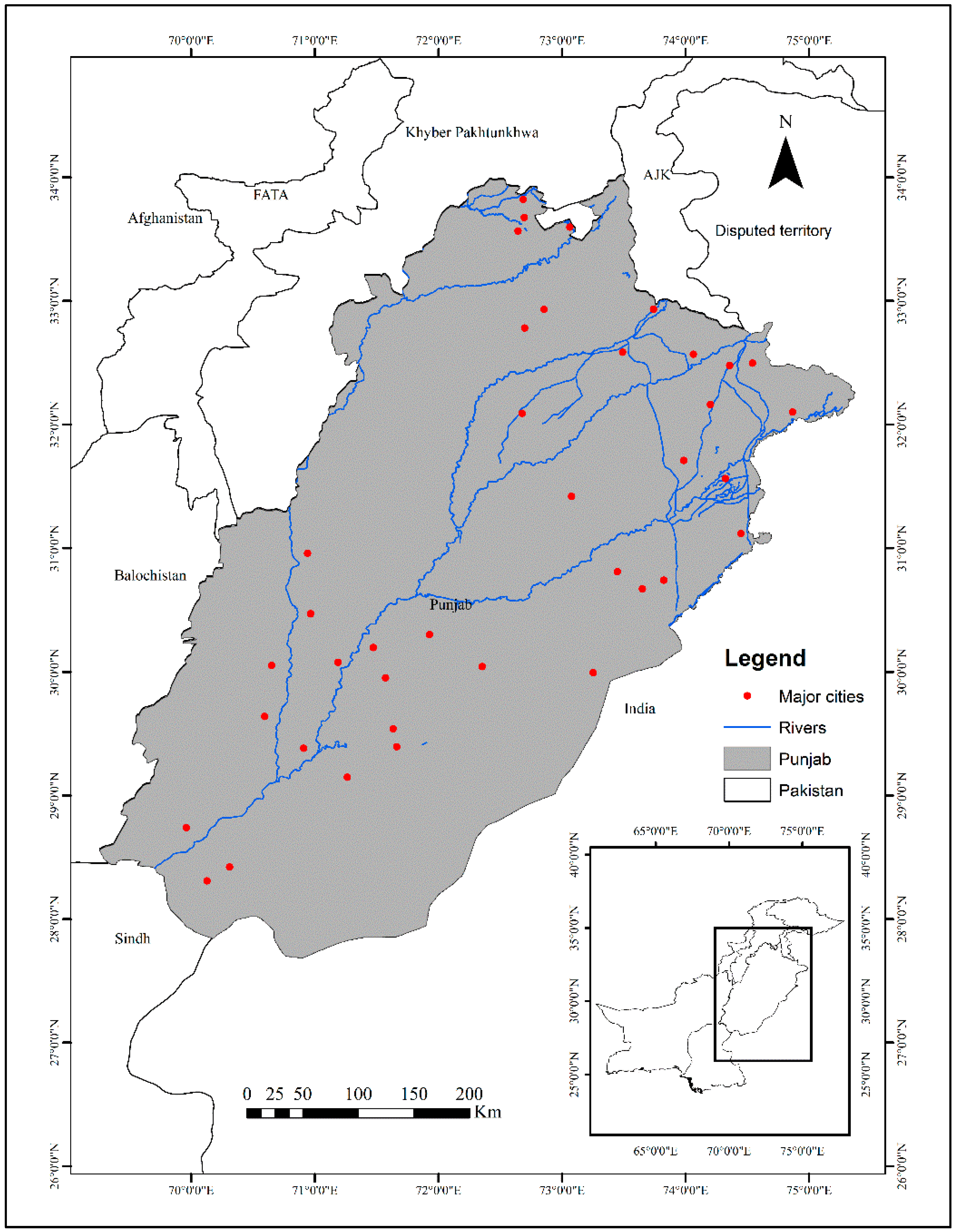
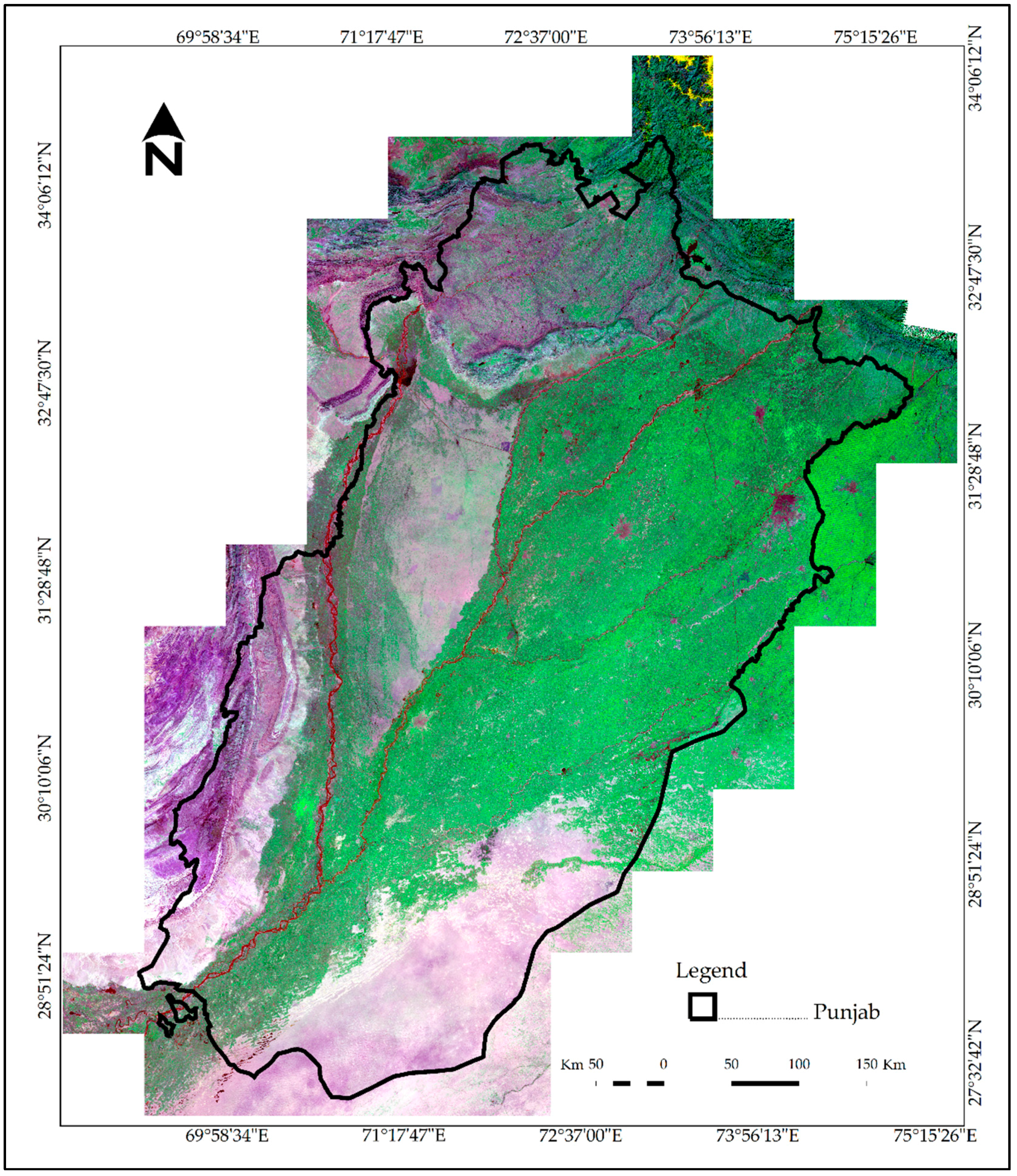
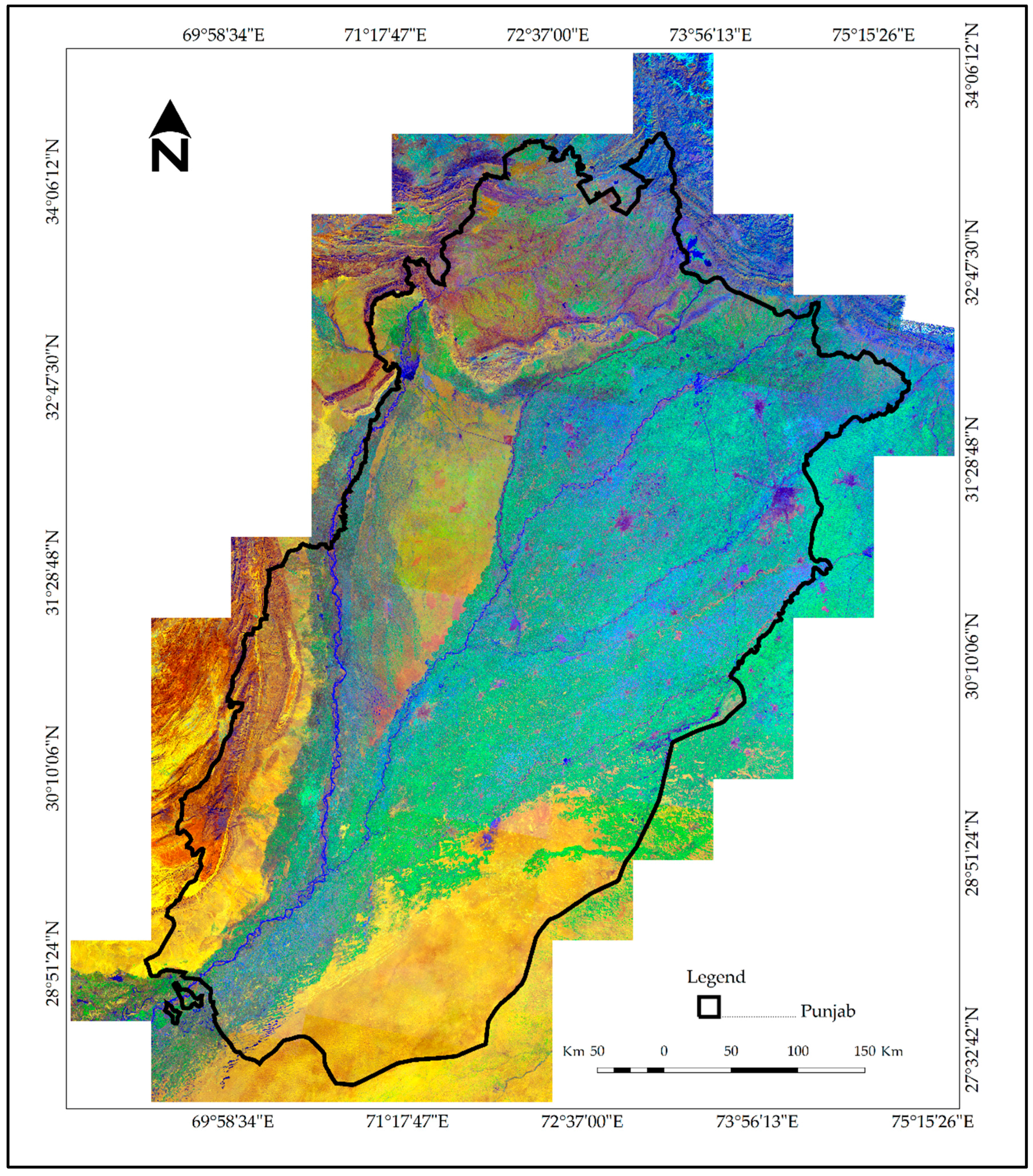
2.1. Study Area
2.2. Data and Methods
2.2.1. Remotely Sensed Data
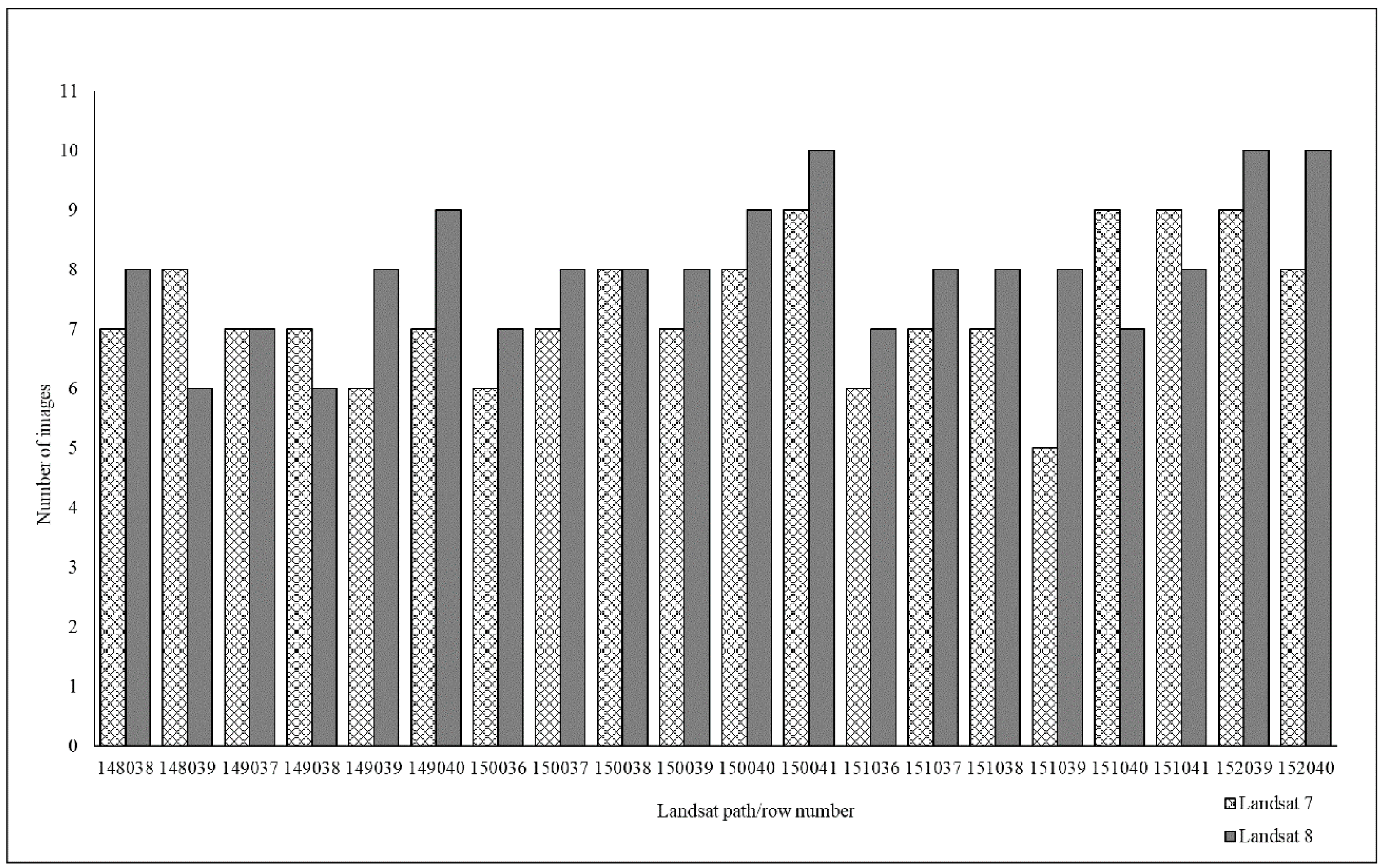
Landsat Data
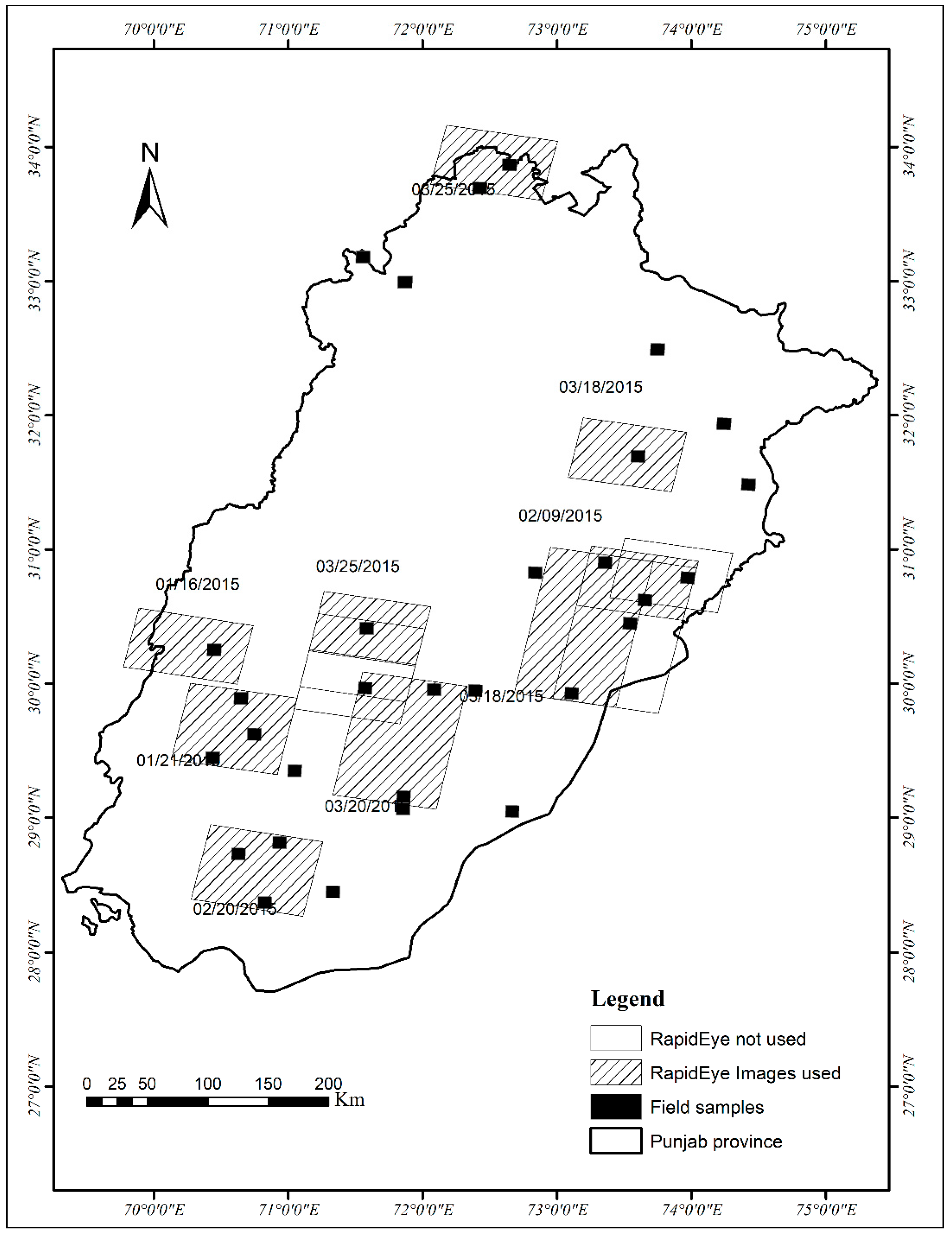
RapidEye Data
Topographic Data
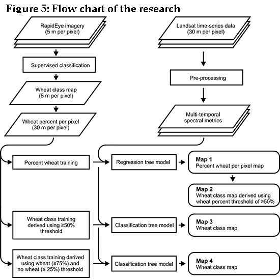
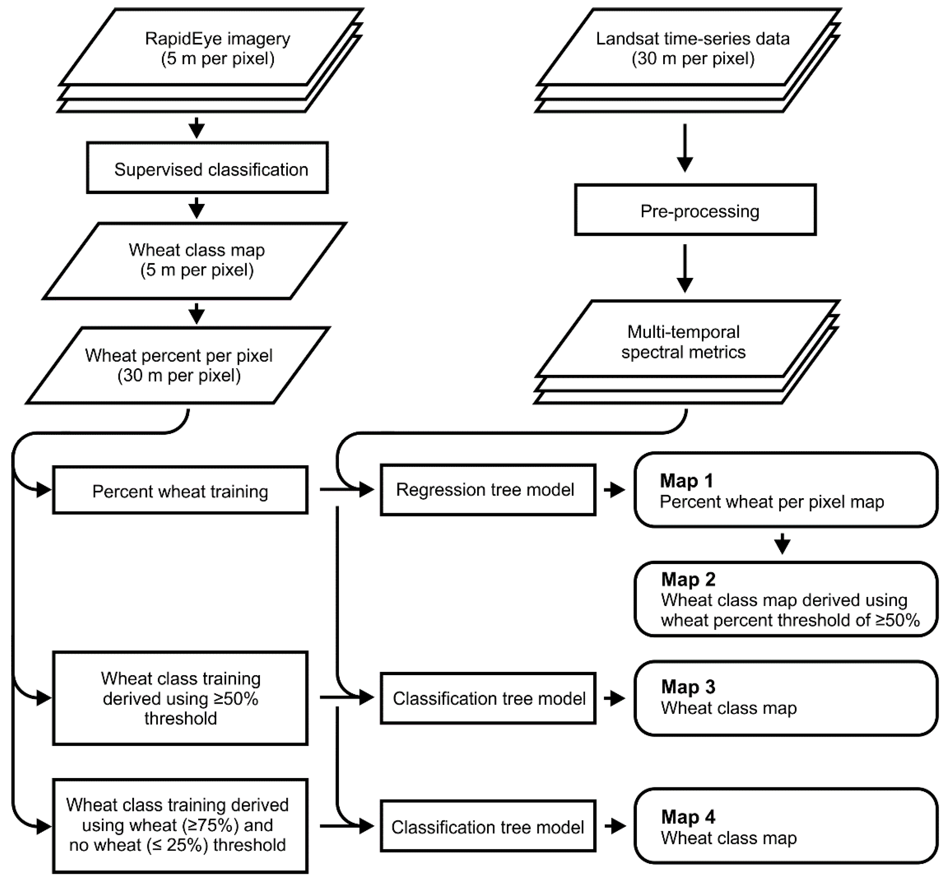
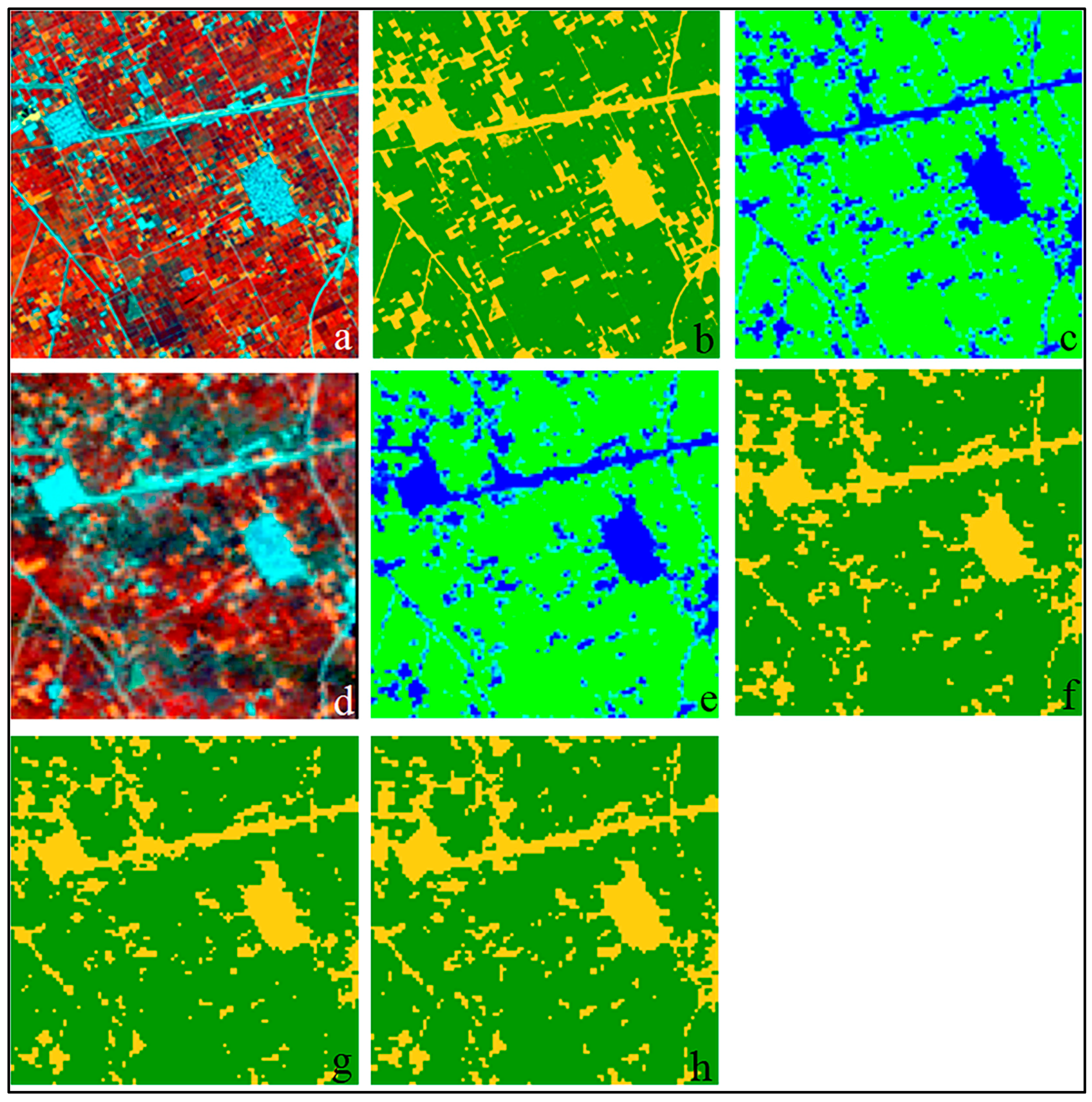
2.2.2. Wheat Mapping: Regression and Classification Trees
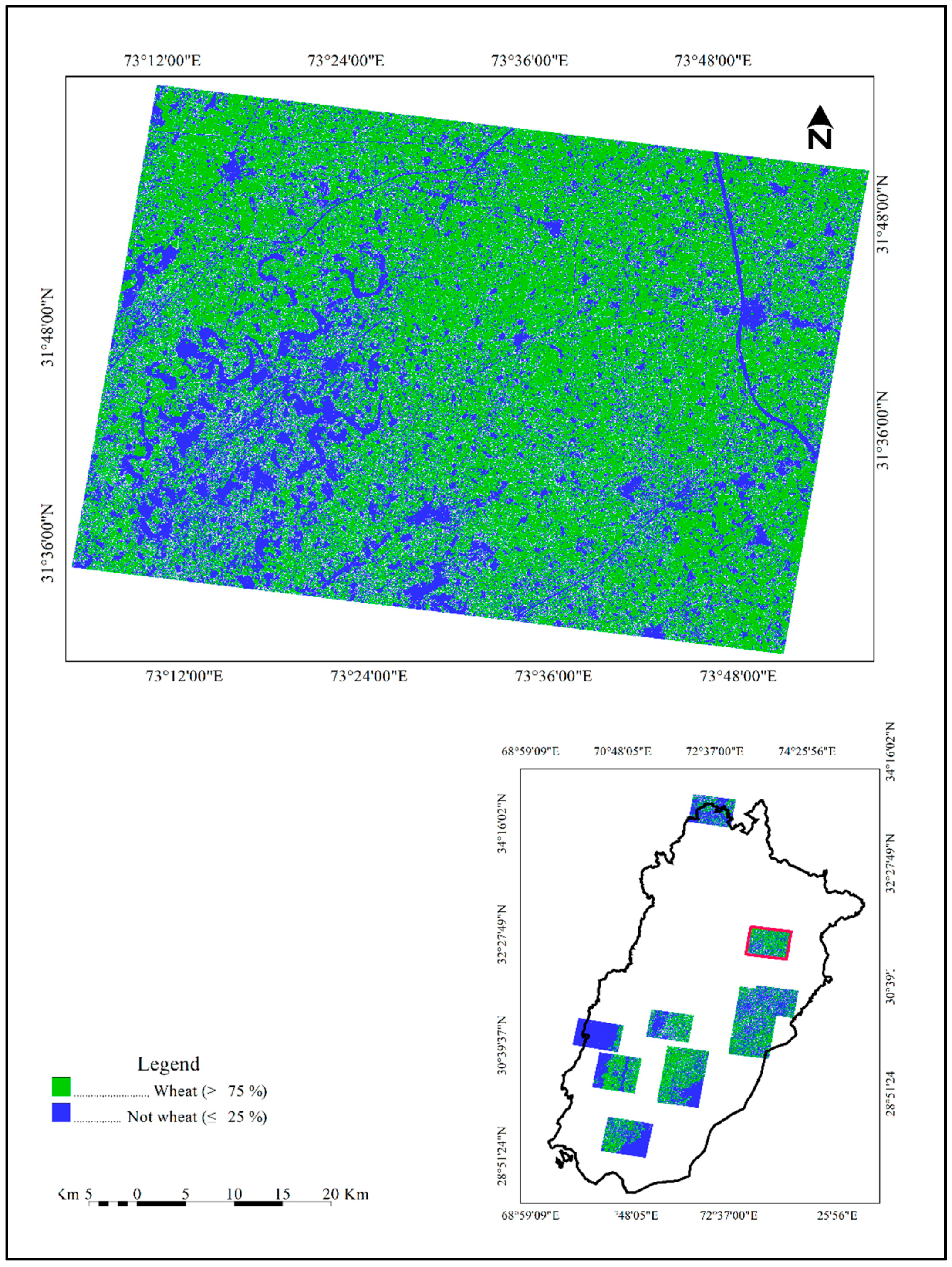
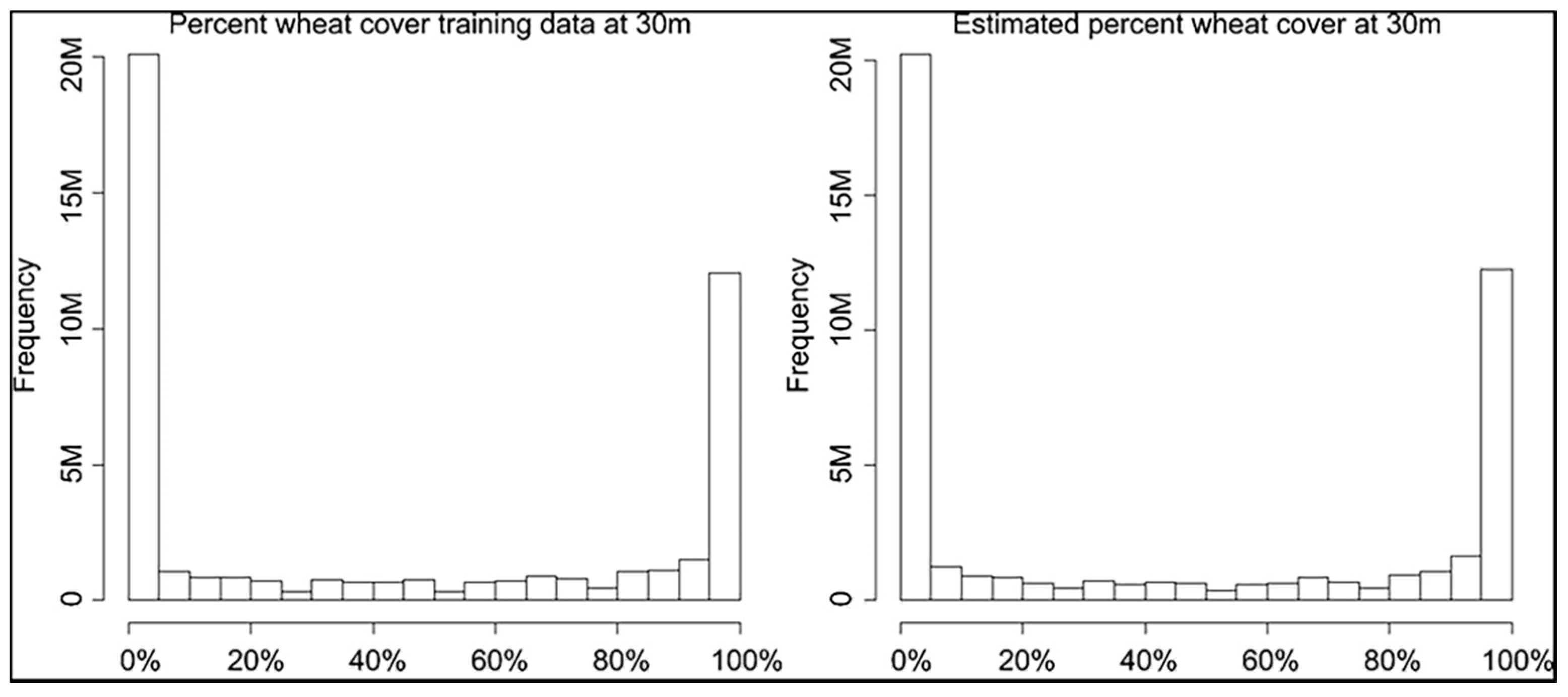
RapidEye-Derived Training Data
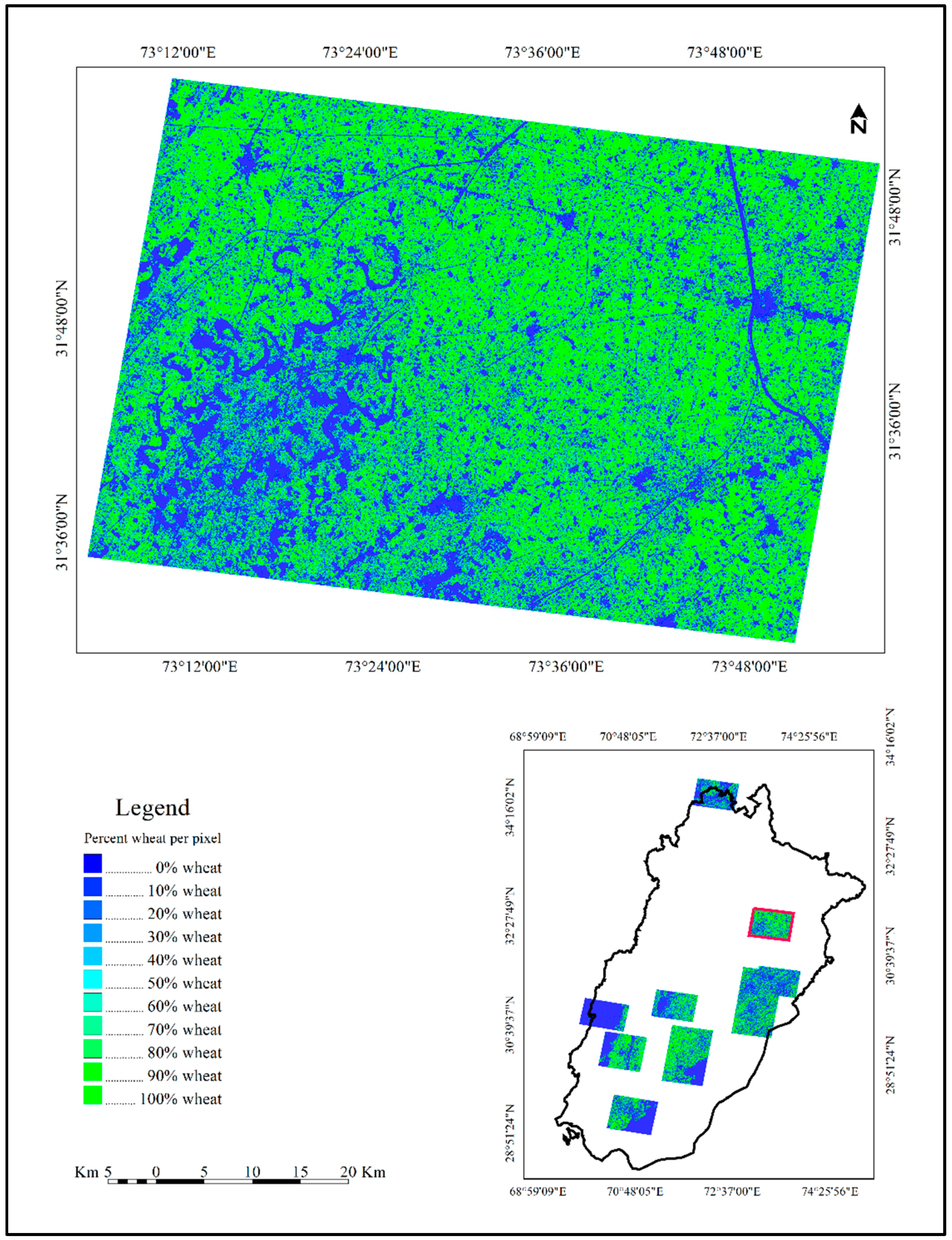
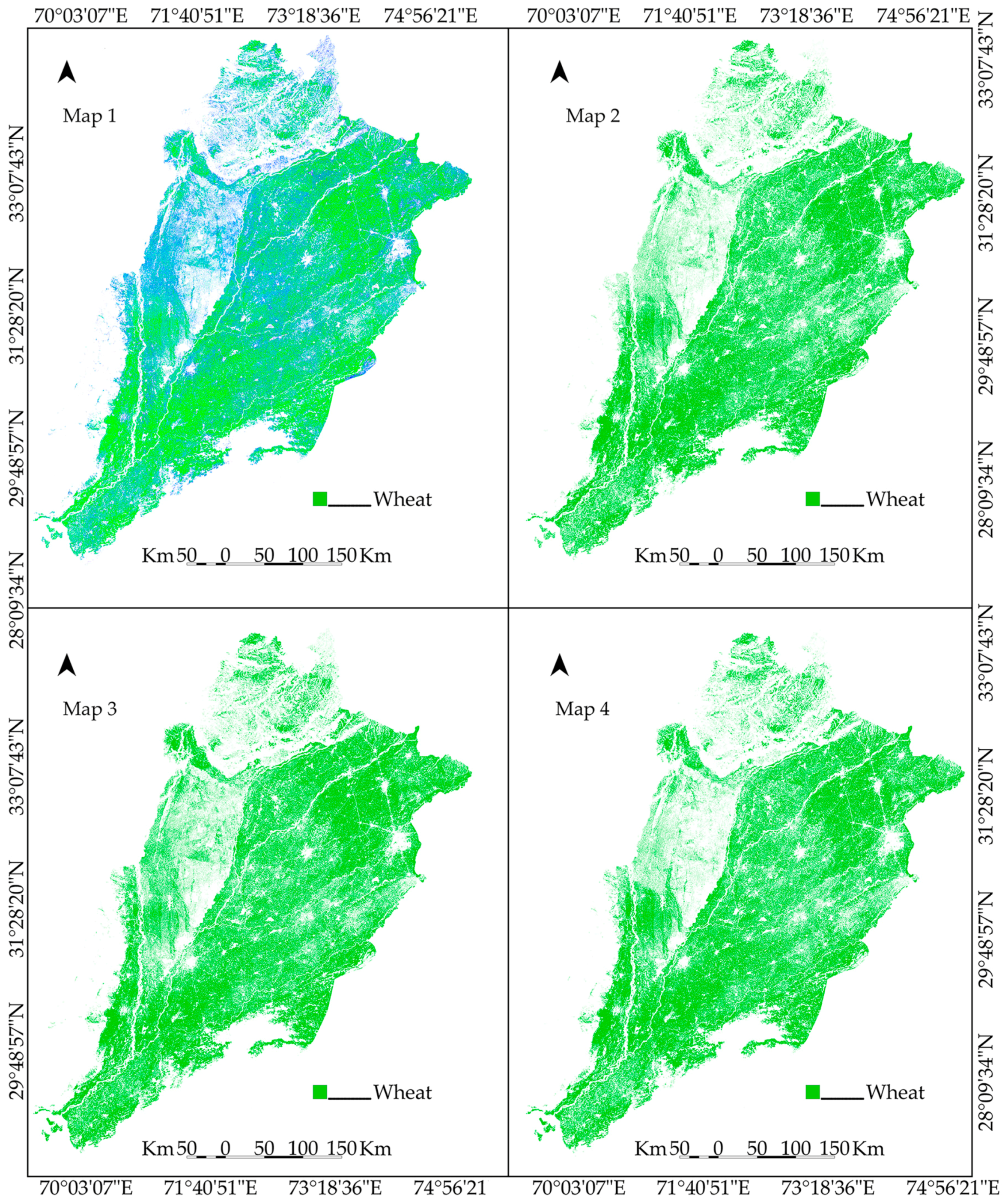
Landsat-Derived Map Products
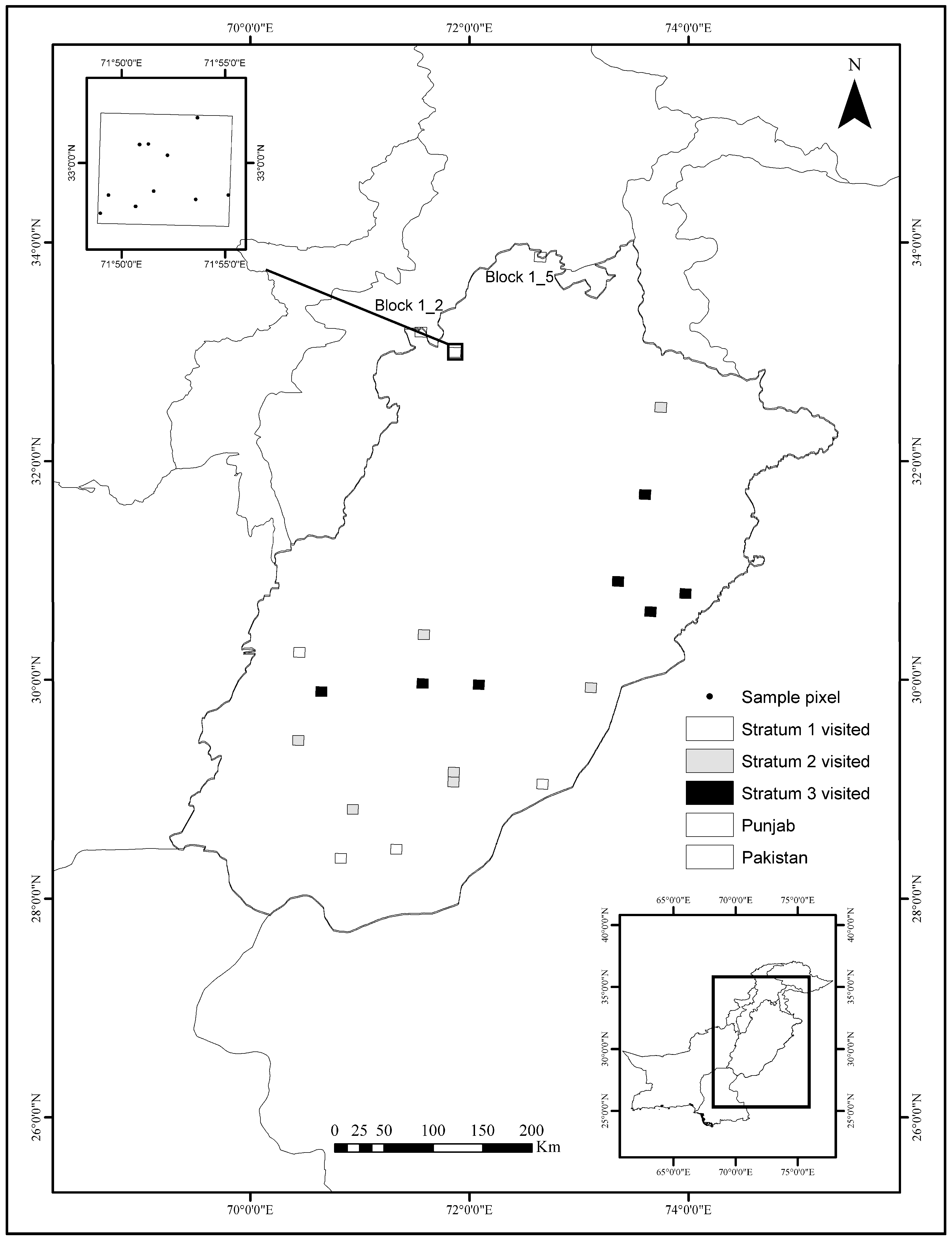
In Situ Data for Area Estimation and Map Validation
3. Results
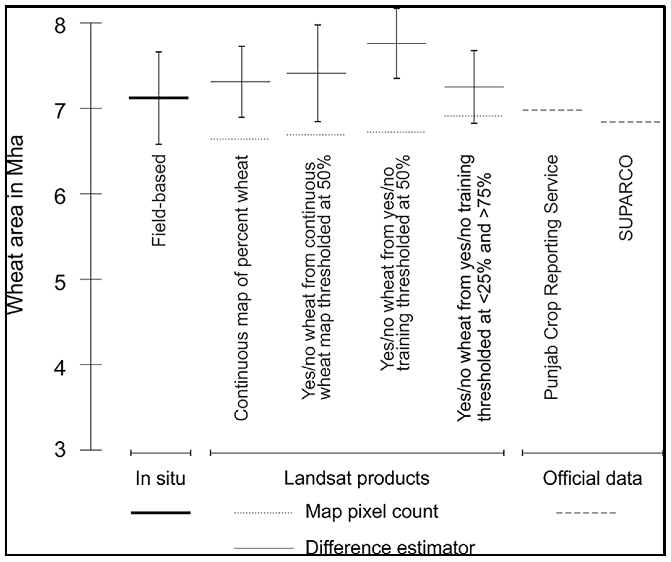
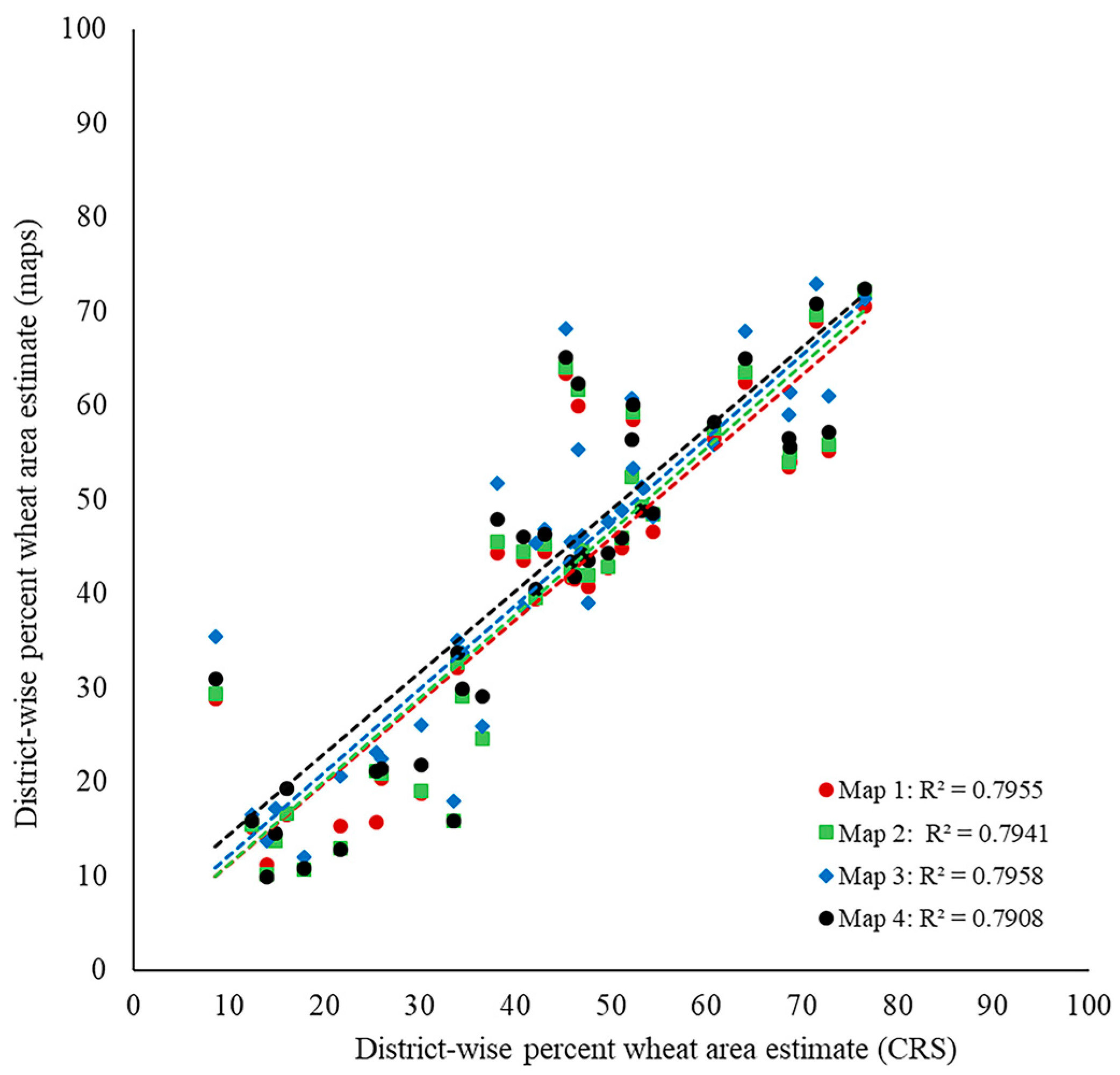
3.1. Intercomparison of Wheat Area Estimates
3.2. Accuracy of the Wheat Maps
4. Discussion
5. Conclusions
Acknowledgments
Author Contributions
Conflicts of Interest
References
- Junior, J.Z.; Coltri, P.P.; Goncalves, R.R.D.V.; Romani, L.A.S. Mult-resolution in remote sensing for agricultural monitoring: A review. Rev. Bras. Cartogr. 2014, 66, 1517–1529. [Google Scholar]
- King, L.; Adusei, B.; Stehman, S.V.; Potapov, P.; Song, X.-P.; Krylov, A.; Di Bella, C.; Loveland, T.; Johnson, D.M.; Hansen, M.C. A multi-resolution approach to national-scale cultivated area estimation of soybean. Remote Sens. Environ. 2017, 195, 13–29. [Google Scholar] [CrossRef]
- Song, X.-P.; Potapov, P.V.; Krylov, A.; King, L.; Di Bella, C.M.; Hudson, A.; Khan, A.; Adusei, B.; Stehman, S.V.; Hansen, M.C. National-scale soybean mapping and area estimation in the United States using medium resolution satellite imagery and field survey. Remote Sens. Environ. 2017, 190 (Suppl. C), 383–395. [Google Scholar] [CrossRef]
- Carfagna, E.; Gallego, F.J. Using Remote Sensing for Agricultural Statistics. Int. Stat. Rev. 2005, 73, 389–404. [Google Scholar] [CrossRef]
- Dempewolf, J.; Adusei, B.; Becker-Reschef, I.; Hansen, M.; Potapov, P.; Khan, A.; Barker, B. Wheat yield forecasting for Punjab Province from Vegetation Index Time Series and Historic Crop Statistics. J. Remote Sens. 2014, 6, 9653–9675. [Google Scholar] [CrossRef]
- Khan, A.; Hansen, C.M.; Potapov, P.; Stehman, S.V.; Chattha, A.A. Landsat-based wheat mapping in the heterogeneous cropping system of Punjab, Pakistan. Int. J. Remote Sens. 2016, 37, 1391–1410. [Google Scholar] [CrossRef]
- Mulla, D.J. Twenty five years of remote sensing in precision agriculture: Key advances and remaining knowledge gaps. Biosyst. Eng. 2013, 114, 358–371. [Google Scholar] [CrossRef]
- GoPakistan. Agricultural Census 2010—Pakistan Report; Pakistan Bureau of Statistics, Government of Pakistan: Lahore, Pakistan, 2010. Available online: www.pbs.gov.pk (accessed on 20 February 2018).
- Zheng, Y.; Wu, B.; Zhang, M.; Zeng, H. Crop Phenology Detection Using High Spatio-Temporal Resolution Data Fused from SPOT5 and MODIS Products. Sensors 2016, 16, 2099. [Google Scholar] [CrossRef] [PubMed]
- The World Bank (WB); Food and Agriculture Organization of the United Nations (FAO). Global Strategy to Improve Agricultural and Rural Statisitcs; WB: Rome, Italy; FAO: Rome, Italy, 2011; p. 39. [Google Scholar]
- Verma, U.; Dabas, D.S.; Hooda, R.S.; Kalubarme, M.H.; Yadav, M.; Grewal, M.S.; Sharma, M.P.; Prawasi, R. Remote sensing based wheat acreage and spectral-trend-agrometeorological Yield Forecasting: Factor Analysis Approach. Stat. Appl. 2011, 9, 1–13. [Google Scholar]
- Heremans, S.; Bossyns, B.; Eerens, H.; Oshoven, J.V. Efficient collection of training data for sub-pixel land cover classification using neural networks. Int. J. Appl. Earth Obs. Geoinf. 2011, 13, 657–667. [Google Scholar] [CrossRef]
- Atzberger, C. Advances in Remote Sensing of Agriculture: Context Description, Existing Operational Monitoring Systems and Major Information Needs. Remote Sens. 2013, 5, 949–981. [Google Scholar] [CrossRef]
- Akhtar, I. Pakistan Needs a New Crop Forecasting System. 2012. Available online: https://www.scidev.net/global/climate-change/opinion/pakistan-needs-a-new-crop-forecasting-system.html (accessed on 16 May 2012).
- Yao, F.; Feng, L.; Zhang, J. Corn Area Extraction by the Integration of MODIS-EVI Time Series Data and China’s Enviornment Satellite (HJ-1) Data. J. Indian Soc. Remote Sens. 2013, 42, 859–867. [Google Scholar] [CrossRef]
- Olofsson, P.; Foody, G.M.; Herold, M.; Stehman, S.V.; Woodcock, C.E.; Wulder, M.A. Good practices for estimating area and assessing accuracy of land change. Remote Sens. Environ. 2014, 148, 42–57. [Google Scholar] [CrossRef]
- SUPARCO. Punjab CRS: Baseline Survey, Agriculture Information System. Building Provincial Capacity for Crop Forecasting and Estimation; A Joint FAO, UN, SUPARCO and Crop Reporting Service; Government of Punjab Publication: Punjab, India, 2012; p. 22.
- Crop Reporting Service, Punjab. Rabi Crop Estimates Data Book 2014–2015; Crop Reporting Service, Punjab: Punjab, India, 2015; p. 86. [Google Scholar]
- Qasim, M. Determinants of Farm Income and Agricultural Risk Management Strategies: The Case of Rain-Fed Farm Households in Pakistan’s Punjab; International Rural Development; Kassel University Press GmbH: Kassel, Germany, 2012; Volume 3, p. 208. [Google Scholar]
- Ministry of Finance, Government of Pakistan. Pakistan Economic Survey 2013–2014; Ministry of Finance, Government of Pakistan: Lahore, Pakistan, 2014. Available online: http://www.finance.gov.pk/survey_1314.html (accessed on 3 July 2014).
- Jabeen, A.; Huang, X.S.; Aamir, M. The Challenges of Water Pollution, Threat to Public Health, Flaws of Water Laws and Policies in Pakistan. J. Water Resour. Protect. 2015, 7, 1516–1526. [Google Scholar] [CrossRef]
- GoPakistan. Provisional Province Wise Population by Sex and Rurual/Urban, 2017th ed.; Government of Pakistan: Pakistan Bureau of Statistics: Lahore, Pakistan, 2017; p. 13. Available online: www.pbs.gov.pk (accessed on 1 April 2015).
- Branca, G.; McCarthy, N.; Lipper, L.; Jolejole, M.C. Climate-Smart Agriculture: A Systhesis of Empirical Evidence of Food Security and Mitigation Benefits from Improved Cropland Management; FAO: Rome, Italy, 2011; p. 36. [Google Scholar]
- Dempewolf, J.; Adusei, B.; Becker-Reschef, I.; Barker, B.; Potapov, P.; Hansen, M.; Justice, C. Wheat Production Forecasting for Pakistan from Satellite Data. In Proceedings of the 2013 IEEE International on Geoscience and Remote Sensing Symposium (IGARSS), Melbourne, Australia, 21–26 July 2013; pp. 3239–3242. [Google Scholar]
- Ouaidrari, H.; Vermote, F.E. Operational Atmospheric Correction of Landsat TM Data. Remote Sens. Environ. 1999, 70, 4–15. [Google Scholar] [CrossRef]
- Tucker, C.J. Photographic Infrared Linear Combinations for Monitoring Vegetation. Remote Sens. Environ. 1979, 8, 127–150. [Google Scholar] [CrossRef]
- Gao, B. NDWI—A normalized difference water index for remote sensing of vegetation liquid water from space. Remote Sens. Environ. 1996, 58, 258–266. [Google Scholar] [CrossRef]
- Potapov, P.V.; Turubanova, S.A.; Hansen, M.C.; Adusei, B.; Broich, M.; Altstatt, A.; Mane, L.; Justice, C.O. Quantifying forest cover loss in Democratic Republic of the Congo, 2000–2010, with Landsat ETM plus data. Remote Sens. Environ. 2012, 122, 106–116. [Google Scholar] [CrossRef]
- Chander, G.; Markham, B.L.; Helder, D.L. Summary of current radiometric calibration coefficients for Landsat MSS, TM, ETM+, and EO-1 ALI sensors. Remote Sens. Environ. 2009, 113, 893–903. [Google Scholar] [CrossRef]
- Hansen, M.C.; Roy, D.P.; Lindquist, E.; Adusei, B.; Justice, C.O.; Altstatt, A. A method for integrating MODIS and Landsat data for systematic monitoring of forest cover and change in the Congo Basin. Remote Sens. Environ. 2008, 112, 2495–2513. [Google Scholar] [CrossRef]
- Hansen, M.; DeFries, R. Detecting long-term global forest change using continuous fields of tree cover maps from 8-km Advanced Very High Resolution Radiometer (AVHRR) data for the years 1982–1999. Ecosystems 2004, 7, 695–716. [Google Scholar] [CrossRef]
- Chang, J.; Hansen, M.C.; Pttman, K.; Dimiceli, C.; Carroll, M. Corn and soybean mapping in the United States using MODIS time-series data sets. Am. Soc. Agron. 2007, 99, 1654–1664. [Google Scholar] [CrossRef]
- DeFries, R.S.; Field, C.B.; Fung, I.; Justice, C.O.; Los, S.; Matson, P.A.; Matthews, E.; Mooney, H.A.; Potter, C.S.; Sellers, P.J.; et al. Mapping the land surface for global atmospher-biosphere models: Toward continous distributions of vegetation’s functional properties. J. Geophys. Res. 1995, 100, 20867–20882. [Google Scholar] [CrossRef]
- Reed, B.C.; Brown, J.F.; VenderZee, D.; Loveland, T.R.; Merchant, J.W.; Ohlen, D.O. Measuring phenological variability from satellite imagery. J. Veg. Sci. 1994, 5, 703–714. [Google Scholar] [CrossRef]
- Pittman, K.; Hansen, M.; Becker-Reschef, I.; Potapov, P.V.; Justice, C.P. Estimating Global Cropland extent with Multi-year MODIS Data. Remote Sens. 2010, 2, 1844–1863. [Google Scholar] [CrossRef]
- Stoll, E.; Konstanski, H.; Anderson, C.; Douglas, K.; Oxfort, M. The RapidEye Constellation and Its Data Products. In Proceedings of the 2012 IEEE on Aerospace Conference, Big Sky, MT, USA, 3–10 March 2012; p. 9. [Google Scholar]
- Arnette, J.T.; Coops, N.C.; Daniels, L.D.; Falls, R.W. Detecting forest damage after a low severity fire using remote sensing at multiple scale. Int. J. Appl. Earth Obs. Geoinf. 2015, 35, 239–246. [Google Scholar] [CrossRef]
- Atzberger, C.; REmbold, F. Mapping the Spatial Distribution of Winter Crops at Sub-Pixel Level Using AVHRR NDVI Time Series and Neural Nets. Remote Sens. 2013, 5, 1335–1354. [Google Scholar] [CrossRef] [Green Version]
- Crnojevic, V.; Lugonija, P.; Brkljac, B.; Brunet, B. Classification of small agricultural fields using combined Landsat-8 and RapidEye imagery: Case study of northern Serbia. J. Appl. Remote Sens. 2014, 8, 1–18. [Google Scholar] [CrossRef]
- Schuster, C.; Forster, M.; Kleinschmit, B. Testing the red edge channel for improving land-use classifications based on high-resolution multi-spectral satellite data. Int. J. Remote Sens. 2012, 33, 5583–5599. [Google Scholar] [CrossRef]
- Breiman, L. Bagging predictors. Mach. Learn. 1996, 24, 123–140. [Google Scholar] [CrossRef]
- Hansen, M.; Dubayah, R.; DeFries, R. Classification trees: An alternative to traditional land cover classifiers. Int. J. Remote Sens. 1996, 17, 1075–1081. [Google Scholar] [CrossRef]
- Bwangoy, J.-R.B.; Hansen, M.C.; Potapov, P.; Turubanova, S.; Lumbuenamo, R.S. Identifying nascent wetland forest conversion in the Democratic Republic of the Congo. Wetl. Ecol. Manag. 2013, 21, 29–43. [Google Scholar] [CrossRef]
- Ripley, B.D. Pattern Recognition and Neural Networks; Cambridge University Press: New York, NY, USA, 1996. [Google Scholar]
- Hansen, C.M.; Egorov, E.; Roy, D.P.; Potapov, P.; Ju, J.; Turubanova, S.; Kommareddy, I.; Loveland, T.R. Continous fields of land cover for the conterminous United States using Landsat data: First results from the Web-Enabled Landsat Data (WELD) project. Remote Sens. Lett. 2011, 2, 279–288. [Google Scholar] [CrossRef]
- Bwangoy, J.-R.B.; Hansen, M.C.; Roy, D.P.; De Grandi, G.; Justice, C.O. Wetland mapping in the Congo Basin using optical and radar remotely sensed data and derived topographical indices. Remote Sens. Environ. 2010, 114, 73–86. [Google Scholar] [CrossRef]
- Breiman, L.; Friedman, J.; Olshen, R.; Stone, C. Classification and Regression Trees; Wadsworth and Brooks/Cole: Monterey, CA, USA, 1984. [Google Scholar]
- Hansen, C.M.; DeFries, R.; Townshend, J.R.G.; Marufu, L.; Sohlberg, R. Development of a MODIS percent tree cover validation data set for Western Province, Zambia. Remote Sens. Environ. 2002, 83, 320–335. [Google Scholar] [CrossRef]
- Becker-Reshef, I.; Vermote, E.; Lindeman, M.; Justice, C. A generalized regression-based model for forecasting winter wheat yields in Kansas and Ukraine using MODIS data. Remote Sens. Environ. 2010, 114, 1312–1323. [Google Scholar] [CrossRef]
- Potapov, P.V.; Dempewolf, J.; Talero, Y.; Stehman, S.V.; Vargas, C.; Rojas, E.J.; Castillo, D.; Mendoza, E.; Calderon, A.; Giudice, R.; et al. National satellite-based humid tropical forest change assessment in Peru in support of REDD+ implementation. Environ. Res. Lett. 2014, 9, 124012. [Google Scholar] [CrossRef]
- Sarndal, C.-E.; Swensson, B.; Wretman, J. Model Assisted Survey Sampling; Springer: New York, NY, USA, 1992. [Google Scholar]
- SUPARCO. Rabi Crop 2014–15; Pakistan Space and Upper Atmosphere Research Commission (SUPARCO): Karachi, Pakistan, 2015; p. 24.


| Sr. # | RapidEye Image Acquisition Date | Image ID | Season |
|---|---|---|---|
| 1. | 16 January 2015 | 23434141_326753 | Early growth stage |
| 2. | 31 January 2015 | 23433903_326754 | Before peak season |
| 3. | 09 February 2015 | 23433753_326753 | Peak growing season |
| 4. | 20 February 2015 | 23434179_326753 | Peak growing season |
| 5. | 18 March 2015 | 23434146_326755 | Late growing season |
| 6. | 18 March 2015 | 23434725_326754 | Late growing season |
| 7. | 20 March 2015 | 23434185_326753 | Late growing season |
| 8. | 25 March 2015 | 23433892_326753 | Before harvest |
| 9. | 25 March 2015 | 23433908_326754 | Before harvest |
| Map Product | Overall Accuracy (%) (SE) | User Accuracy (%) | Producer Accuracy (%) | Wheat Area (Mha) from Difference Estimator (Standard Error) | ||
|---|---|---|---|---|---|---|
| Wheat (SE) | No-Wheat (SE) | Wheat (SE) | No-Wheat (SE) | |||
| Continuous map of percent wheat derived from RapidEye percent wheat training (Map 1) | 88 (4) | 87 (3) | 89 (5) | 79 (9) | 94 (2) | 7.31 (0.83) |
| Binary map of wheat/no wheat derived from continuous wheat map thresholded at 50% (Map 2) | 90 (4) | 90 (3) | 90 (5) | 80 (8) | 95 (2) | 7.41 (1.13) |
| Binary map of wheat/no wheat derived from wheat/no wheat RapidEye training thresholded at 50% (Map 3) | 90 (4) | 91 (3) | 90 (5) | 81 (8) | 96 (2) | 7.76 (0.82) |
| Binary map of wheat/no wheat derived from yes/no RapidEye training thresholded at ≤25% and ≥75% (Map 4) | 87 (4) | 84 (5) | 88 (6) | 77 (8) | 92 (2) | 7.25 (0.85) |
© 2018 by the authors. Licensee MDPI, Basel, Switzerland. This article is an open access article distributed under the terms and conditions of the Creative Commons Attribution (CC BY) license (http://creativecommons.org/licenses/by/4.0/).
Share and Cite
Khan, A.; Hansen, M.C.; Potapov, P.V.; Adusei, B.; Pickens, A.; Krylov, A.; Stehman, S.V. Evaluating Landsat and RapidEye Data for Winter Wheat Mapping and Area Estimation in Punjab, Pakistan. Remote Sens. 2018, 10, 489. https://doi.org/10.3390/rs10040489
Khan A, Hansen MC, Potapov PV, Adusei B, Pickens A, Krylov A, Stehman SV. Evaluating Landsat and RapidEye Data for Winter Wheat Mapping and Area Estimation in Punjab, Pakistan. Remote Sensing. 2018; 10(4):489. https://doi.org/10.3390/rs10040489
Chicago/Turabian StyleKhan, Ahmad, Matthew C. Hansen, Peter V. Potapov, Bernard Adusei, Amy Pickens, Alexander Krylov, and Stephen V. Stehman. 2018. "Evaluating Landsat and RapidEye Data for Winter Wheat Mapping and Area Estimation in Punjab, Pakistan" Remote Sensing 10, no. 4: 489. https://doi.org/10.3390/rs10040489