Detecting Forest Road Wearing Course Damage Using Different Methods of Remote Sensing
by
 , ,
, ,
Petr Hrůza
1,*, 
Tomáš Mikita
2,*,
Nataliya Tyagur
3,
Zdenek Krejza
4,
Miloš Cibulka
2,
Andrea Procházková
2 and
Zdeněk Patočka
2 1
Department of Landscape Management, Faculty of Forestry and Wood Technology, Mendel University in Brno, Zemědělská 3, 613 00 Brno, Czech Republic
2
Department of Forest Management and Applied Geoinformatics, Faculty of Forestry and Wood Technology, Mendel University in Brno, Zemědělská 3, 613 00 Brno, Czech Republic
3
Institute of Geodesy, Faculty of Civil Engineering, Brno University of Technology, Veveri 331/95, 602 00Brno, Czech Republic
4
Centre AdMaS, Faculty of Civil Engineering, Brno University of Technology, Purkyňova 651/139, 612 00 Brno, Czech Republic
*
Authors to whom correspondence should be addressed.
Remote Sens. 2018, 10(4), 492; https://doi.org/10.3390/rs10040492
Submission received: 17 January 2018
/
Revised: 6 March 2018
/
Accepted: 19 March 2018
/
Published: 21 March 2018
Abstract
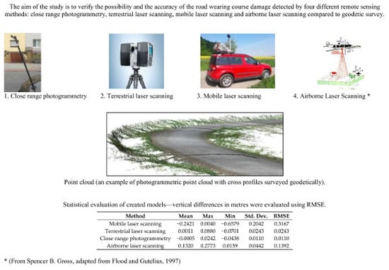
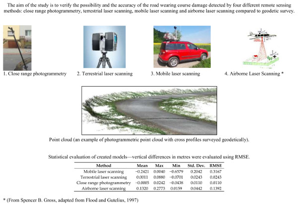
:Currently, a large part of forest roads with a bituminous surface course constructed in the Czech Republic in the second half of the last century has been worn out. The aim of the study is to verify the possibility and the accuracy of the road wearing course damage detected by four different remote sensing methods: close range photogrammetry, terrestrial laser scanning, mobile laser scanning and airborne laser scanning. At the beginning of verification, cross sections of the road surface were surveyed geodetically and then compared with the cross sections created in the DTMs which were acquired using the four methods mentioned above. The differences calculated between particular models and geodetic measurements show that close range photogrammetry achieved an RMSE of 0.0110 m and the RMSE of terrestrial laser scanning was 0.0243 m. Based on these results, we can conclude that these two methods are sufficient for the monitoring of the asphalt wearing course of forest roads. These methods allow precise and objective localization, size and quantification of the road damage. By contrast, mobile laser scanning with an RMSE of 0.3167 m does not reach the required precision for the damage detection of forest roads due to the vegetation that affects the precision of the measurements. Similar results are achieved by airborne laser scanning, with an RMSE of 0.1392 m. As regards the time needed, close range photogrammetry appears to be the most appropriate method for damage detection of forest roads.
1. Introduction
There are two current approaches to data collection and road condition monitoring. Manual data collection used in many countries is slow and it provides poor data [1]. The most common method of measurement is still the geodetic method, with the use of a total station in combination with Global Navigation Satellite System (GNSS). In connection with the use of GNSS, Abdie et al. [2] published an article on the accuracy and the usability of the technology for forest road mapping in the forest environment. According to the article, the forest road network inventory using GNSS is a method often used due to its relatively low purchase price. In line with other authors [3], they state that the utilization of GNSS in the forest ecosystem brings problems with signal reception under the forest cover, including the fact that a different number of satellites is visible in the territory at different times.
Remote sensing technologies have also been commonly used in many applications during the last fifteen years. The derived three-dimensional data are regularly used for digital terrain and surface modelling. Detailed information about roads and their surroundings is very important because of the ever-increasing number of applications, such as noise modelling, traffic safety, road maintenance and repair, driver assistance, or car and pedestrian navigation [4].
Recently, methods of automated data collection and the already mentioned remote sensing methods have become increasingly widespread with the development of new technologies [5,6,7]. The modelling technology for obtaining 3D information can be divided by the used mapping method [4]. According to [8], Light Detection and Ranging (LiDAR) is currently the most sophisticated method for the exploration of the forest road network. LiDAR is a method of distance measurement based on the speed calculation of the reflected laser beam pulse from the scanned object. The method is primarily used for the creation of a digital terrain model (DTM).
The LiDAR method is mostly used as airborne laser scanning (ALS) in which the scanner is mounted on an aircraft. ALS is increasingly used for city modelling, for the generation of digital terrain models, archeological studies [9] or for forest inventory [10,11,12,13]. The distance of the airborne scanner from the scanned location on the Earth’s surface is several hundred metres or several kilometres. According to [3], the density of the obtained points (1–20 b/m2) is sufficiently high for a rough extraction of the contour and the structure of building roofs. However, it is not sufficient for their detailed modelling or for detailed modelling of the road surfaces; for example, road wearing course damage or road debris cannot be detected and modelled.
In the field of opening-up forests, ALS was used to determine the layout of the forest roads within forest stands with an accuracy of one to two metres [8,14]. The method can facilitate the updating of the forest road network maps, increase the efficiency of the accessibility and it can be used to plan harvesting and transport processes, e.g., the layout and the lengths of skidding and hauling roads. Nevertheless, data processing may be more time consuming and not applicable for more accurate and detailed data on road wearing course damage.
Saito et al. [15] published an article on the possible use of the ALS method for the automatic design of a forest road network that takes into account negative points for its layout, such as sites threatened by landslides. Based on accurate DMT created using LiDAR data, it is also possible to localize the drainage objects on the forest roads and minimize the erosion resulting from the construction of forest roads [16]. Contreras et al. [17] attempted to use the created DMT to determine the extent of groundworks during a hauling road design and compared its precision with the data obtained by the conventional ground-based method. Aricak et al. [18] used the commercial satellite imagery system GeoEye-1 with high spatial resolution of 0.46 m pixels to create the DTM. However, the resulting definitions of about 1 meter cannot be used to evaluate the status of the wearing course [19].
In addition to airborne laser scanning, terrestrial laser scanning (TLS) and mobile laser scanning (MLS) can also be used. These methods provide a greater point cloud density, up to thousands of points per m2. The TLS method is one of the most progressively developing methods of 3D data acquisition. Nowadays, the TLS can be applied in various fields: topographical measurements [20], exploration of landslides [21,22], forest inventory [23,24,25], documentation of the actual state of buildings [26,27,28], mapping of industrial sites and underground areas [20,29], monitoring of ground surface erosion [30], documentation of cultural heritage [31,32,33,34], and many others.
The use of such technology can provide a large amount of up-to-date high-resolution data over a short period and it enables very accurate modelling of the environment. Laser scanners use various methods for data acquisition, such as triangulation, Time of Flight (TOF), Phase-Shift [35]. A 3D laser scanner with the triangulation method based on a line-laser is used for very short range scans and collects data to micron level accuracy. This system is mainly used in engineering applications, in archeology, and in precise scanning of the texture on road pavements [36]. A TOF 3D laser scanner measures the time duration in which a laser travels between the scanner and the object so that the space resolution depends on the accuracy of measuring time [23]. According to [23], these characteristics allow very long measurement distances, but relatively low acquisition speeds. This method is well suited to 3D reconstruction of scenes at larger distances [23] and for large areas or objects [35]. A phase-shift type determines the position of points based on the continual measurement of the phase shift between the laser beams transmitted and received. Due to their range, phase-shift based scanners are well suited for high precision and detailed measurements of relatively near scenes [23]. This method enables very fast surface data obtaining (up to million points per second). The phase-shift scanners are generally faster, more accurate and versatile than the TOF scanners.
The TLS technology can be effectively used for a road surface survey before reconstruction, together with documentation of the current condition to detect damage (e.g., rutting, potholes) or to determine the amount of material needed for the road repair. Moreover, the TLS can be used to generate a model for the milling quality control and subsequent laying of a new surface layer. There are studies [37,38,39] that dealt with the assessment of road surface inequalities and road shape analysis. The main problem of the surface of roads, including forest roads, is rut development [40]. Water flowing in these ruts concentrates in some places, the road surface is flooded and subsequent freezing causes surface damage [41]. These deformations on the road surface affect the gradual disintegration of the forest road surfaces, which require more frequent repairs [42].
The main advantage of TLS is rapid and easy non-contact collection of high-precision data with very high resolution obtained in an optimal quantity/time ratio (thousands of points per second) [43]. Due to the advantages, especially high-precision data collection, TLS technology can be used in the field of road construction to monitor the wear of the road surface [40]. Forest roads should always have a stable and quality surface for safe driving. Therefore, expensive periodic maintenance and repairs of forest roads are carried out [40].
Mobile laser scanning (MLS) systems are widely used in urban areas, especially for scanning and evaluation of paved roads. The scanning process is fast and easy and it allows obtaining very dense point clouds precisely representing reality. That is why it is widely used in transportation management, extraction of the road objects, and even for monitoring of natural objects. For example, Jaakkola et al. [44] presented automatic methods for road marking and kerbstone classification; Bitenc et al. [45] used MLS for monitoring of a sandy coast; Wang et al. [46] used roadside environment from MLS data to model water flow. It has also been used to evaluate road traffic safety by analysing pavement cracks [47] or road roughness detection [48]. A mobile scanner can also be placed on a vessel and used, for example, for mapping rivers or shore erosion [49,50,51]. According to [52], MLS can collect 3-dimensional road and road-related geospatial information accurately and efficiently. Their paper provides a complete workflow for the detection and classification of pole-like road objects from MLS in a motorway environment. In article [53], the authors present a method for estimating the condition of a road using the MLS measurement technique. They state that the application of MLS could provide valuable proof of the road technical condition. Vallet et al. [54] propose a pipeline to produce road orthophotos and DTM from MLS, as for DTM, MLS offers a much higher accuracy and density than aerial products. However, most of these studies deal with civil engineering in urban areas for traffic and city planning and modeling. Kukko et al. [55] present multiplatform MLS solutions for mapping applications that require mobility in various terrains and river environments but produce high density point clouds with good reliability and accuracy. They used MLS under difficult measurement conditions such as the sea or river with accurate information over a large open area, which is in contrast with our study.
There are different approaches and algorithms for DTM generation from MLS data in urban or rural areas [56,57,58]. In our work, the robust filtering algorithm in combination with hierarchical interpolation [59,60,61] was used to generate the DTM from the MLS data. The algorithm has proved to be one of the efficient algorithms for generating DTM in forest areas. The algorithms were applied in software OPALS [62,63,64]. Unfortunately, mobile laser scanning of forest roads remains challenging due to the low GNSS signal and the airborne laser scanner cannot always get through the dense canopy.
Nowadays, photogrammetric image processing is commonly used for creating 3D models of objects such as buildings and trees even in large areas, so it is possible to map the structure of forest stands, for example. The Structure from Motion (SfM) algorithm is the most frequently used for the processing. This photogrammetric method is designed for creating three-dimensional models of a feature or topography from overlapping two-dimensional photographs taken from many locations and orientations to reconstruct the photographed scene. This technology has existed in various forms since 1979 [65], but applications were uncommon until the early 2000′s. The utilization of SfM is wide-ranging, from many subfields of geoscience (geomorphology, tectonics, structural geology, geodesy, and mining) to archaeology, architecture, and agriculture. In addition to ortho-rectified imagery, SfM produces a dense point cloud dataset that is similar in many ways to that produced by airborne or terrestrial LiDAR.
Hrůza et al. [66] tested the use of SfM technology to detect road damage to a forest path using UAV with high quality results. The results of the tested road section showed that unmanned aircraft systems can be used to detect the forest road surface damage with a difference in accuracy of up to 2 cm compared with the accuracy of the current tachymetric methods. However, Unmanned aerial vehicle (UAV) flight over the forest road carries the risk of collision with the tree crowns and puts high demands on drone control. Therefore, the same author [67] later tested the imaging method using cameras carried on a rod with a steady height of about 3 m. The method achieved similar results; the height differences reached 0.026 m, the X and Y horizontal differences were 0.019 m and 0.029 m, respectively.
The aim of this study is to verify whether it is possible, and with what precision, to detect the damage of the wearing course by means of different 3D imagining methods, which would facilitate and accelerate this process. Four different methods were used for the purpose of the study: mobile laser scanning, terrestrial laser scanning, close-range photogrammetry and airborne laser scanning.
2. Materials and Methods
Comparison of different methods of forest road mapping was carried out on the section of the first-class forest road “Hradská” in the Training Forest Enterprise “Masaryk Forest” Křtiny. The road wearing course surface was constructed from penetration macadam that was broadly used for the reinforcement of forest transport roads, especially in the second half of the last century, during the extensive construction of the forest road network in the Czech Republic. A road section of 580 m was chosen for the purposes of the study (Figure 1). The entire survey was carried out in June 2017.
2.1. Geodetic Survey
First, cross profiles were surveyed in 20 m intervals for the accuracy comparison. A geodetic survey of the cross profile points was carried out using the GNSS receiver Topcon Hiper Pro in combination with the Trimble M3 total station. A point network has been created and point positions measured using GNSS with applied differential RTK (Real Time Kinematic) correction from CZEPOS (Czech Positioning System) permanent stations network. The points were measured in the JTSK coordinate system and the Baltic Vertical Datum—After Adjustment. First, in total, 14 traverse points of polygon were stabilized and measured. Position measurements of the traverse points by GNSS were used exclusively for places with open canopy due to road length and poor GNSS signal. These points served as occupied points and orientation for the total station Trimble M3. The other traverse points were surveyed tachymetrically based on a measured and balanced polygon program. Subsequently, 30 road cross sections (404 detail points) were measured from stabilized traverse points by total station. The points within the cross sections were measured at distances 20 cm apart. Surveying of the road using the tachymetry took 3 h.
2.2. Methods
2.2.1. Close Range Photogrammetry
A GoPro Hero 5 camera placed on the front of a car at a height of about 1.5 m above the ground was used to obtain image data (Figure 2). The camera has a 12 MPX resolution and allows continuous capturing of images (so called Time Lapse Photo) in half-second intervals. During the data collection, the driving speed must be around 10 km/h for at least 70% overlap of the images. Linear width adjustment with the camera’s inclination of about 45° was used in the course of data collection. This adjustment ensures a sufficient full-frame width of the entire road and it is optimal for post-processing in AGISOFT PhotoScan software as well.
For a precise alignment of individual images and creation of a precise digital surface model and orthopedic mosaic, it was necessary to mark out and survey the control points that serve for the scale determination and model georeferencing. In this case, a total of 26 points were placed and measured tachymetrically. These points have been marked with a special template that allows their automatic identification in the photos and reduces manual data processing significantly. All control points for photogrammetry were measured from occupied point using total station tacheometrically. Therefore, accuracy of point positions can be defined as milimetre-level. The imaging itself, including the preparation and assembly of the car holder, took about 10 min. The total time of the survey, counting the measurement of the control points, was less than 2 h.
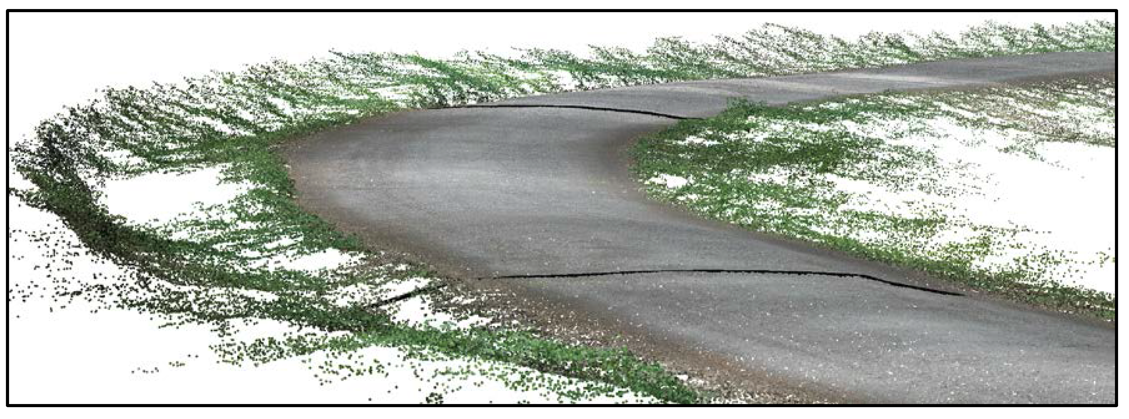
Altogether, 1298 images were captured on the road over a length of 580 m in a period of about 3 min. The images were then processed by AGISOFT PhotoScan software to orthophotographs with 5 cm resolution and to the stereophotogrammetric 3D point cloud with an average density of 4 points per 1 cm2 (Figure 3). The report from AGISOFT PhotoScan showed that created model should have good accuracy with both horizontal and vertical RMSE values to 2 cm. These values were automatically calculated based on the re-validation of control points during image alignment.
The stereophotogrammetric point cloud was then processed in ArcGIS Desktop (version 10.5) by ESRI headquartered in Redlands, CA, USA. 3D Analyst and Spatial Analyst extensions were used for the processing (Figure 3). The first step was to define the boundaries of the forest road wearing course on the basis of manual identification of the roadside over the orthophotograph. In the next step, the stereophotogrammetric point cloud was interpolated using linear interpolation to create continuous raster DTM of the forest road. The created model was generalized to the resolution of 5 cm due to the computational demands of other analyses.
2.2.2. Terrestrial Laser Scanning
The Faro Focus 3D laser scanner was used for the measurement. It is a static panoramic scanner of the “Phase-Shift” type which determines the position of the points based on constant phase shift measurement between the transmitted and received laser beam. The used scanner has a length range of 0.6 m to 120 m. This measurement technology allows high speed data recording (up to 976,000 points per second). Faro Focus 3D uses a wavelength of 905 nm. The accuracy of the length determination is ±2 mm per 10 m. The scanner allows working with different resolution values, ranging from full (1/1) to very low resolution (1/32). A resolution of 1/4 was chosen for the purpose of this study. At such a resolution, scanned points create a point network of approximately 6 mm spacing within 10 m from the scanner. The spacing of the points proportionally increases with increasing distance from the scanner. Depending on the resolution, the number of measurements performed at each point can be set. In this case, the lowest value was set due to considerable time savings. Both values (resolution and quality) were set based on the experience gained from the previous measurements. Such setting combination ensures an appropriate ratio between the scanning velocity (very high) and the density and quality of the obtained data. There were 14 occupied points used for scanning of an approximately 580-m long road. The height of the scanner mounted on a tripod ranged from 1.6 to 1.7 m above the ground. The horizontal and the vertical range of measurements (Field of View) were set to 360°and 300°, respectively. During the scanning, the direction of the scanner was clockwise. Sphere targets or checkboards serving to connect all scans to one common point cloud were placed at each scanning station. The Trimble M3 total station was used for surveying rectangular coordinates (x, y, z) of the eight checkboards in the coordinate system JTSK and the Baltic Vertical Datum - After Adjustment. The measurements were carried out from stabilized occupied points using the Topcon HiPer Pro. The occupied points were measured with of 0.015 m in position and 0.02 m in height. The coordinates of the checkboards are necessary to georeference the resulting point cloud. The scanning time at each point was 1 min and 50 s. The placement of sphere targets and checkboards took about 3 min. Total field measurement time, including measurement of the coordinates, movement and cleaning of the apparatus and the accessories, was approximately 90 min.
The measured data were imported from the SD card of the scanner into the Faro Scene basic processing software (version 5.3) by Faro Technologies. The first step consisted of the automated filtration based on the “Stray” filter to eliminate so-called stray (faulty) points. Subsequently, the points of the individual scans were filtered manually, aligned into one set (point cloud) on the basis of automatic recognition of sphere targets and checkboards, and transformed to the desired coordinate system. Complete processing in the Faro Scene took about 40 min. The resulting georeferenced point cloud was exported to xyz format (Ascii Files) and then converted to LAS format using the “pointzip” tool (version 1.0). Subsequently, LAS points were converted to DTM of 5 cm resolution using the linear interpolation in ArcGIS 10.5 software.
2.2.3. Mobile Laser Scanning
The scanning process was performed by scanner Riegl VMX-450. The measuring head of the scanner consists of two Riegl VQ-450 laser scanners (left and right), IMU and GNSS, which were mounted on a car roof (Figure 4). The measurement rate for each scanner is 550,000 meas./s, with a scan rate of about 200 profiles/s. A single scanner provides a 360° gapless profile, with high accuracy (8 mm) and precision (5 mm). Before the data collection process, the scanner was successfully initialized on the open parking space near the forest. The initialization was done according to the manufacturer’s instructions. The process took nearly 20 min, to achieve good connection with the satellites. The data collection itself took nearly 15 min; the dataset contains 6 LAS files (3 from each scanner). To compute the trajectory and subsequent generation of the point clouds, the data from permanent GNSS stations (30 s sampling) of the EUREF network were used. Georeferencing of the trajectory took place in the Applanix POSPac MMS software. For better alignment, the data from several GNSS stations were used. Additional control points on the terrain were not measured for this method. The data were processed in software OPALS (Orientation and Processing of Airborne Laser Scanning data), developed by Research Groups Photogrammetry and Remote Sensing, Department of Geodesy and Geoinformation, Vienna University of Technology.
The average point density of the collected point cloud is 1029 (pts/m2). Due to the huge capacity of the data, some filtering steps should be applied before running the robust filtering algorithm, which classifies terrain and non-terrain points using robust surface interpolation. Steps of the methodology used for the creation of DTM from MLS data can be divided into:
- Import data into software OPALS and thin each point cloud by choosing the smallest Z-value in every 0.15 m2 cell. Then, six data sets were joined into one for further processing.
- Morphologic filtering (second smallest Z-value in 1 × 1 m cell) and preliminary DTM interpolation (robust moving planes (RMP) and Delaunay triangulation (DT) with a grid size 1m2 both). The DT_dtm was used to fill gaps in RMP_dtm. Then, attribute “normalized Z” was created and added to the point cloud by subtracting the preliminary DTM from the Z-values.
- The third step is the same as the second but with other parameters. Thinning and interpolation were applied for each 0.25 m2 cell. Also, during morphological filtering, we used an asymmetric height threshold from −0.5 to 0.2 m to ensure that all points below the fitted plane will be considered. After interpolating grids, the attribute “normalized Z” was renewed.
- Robust filtering and DTM interpolation. The main parameters of robust filtering are the following: search radius 1 m; plane interpolation; normalized Z below 0.2 m. After we obtained terrain points, we used robust moving plane interpolation to create a DTM with a grid size of 0.05 m for our comparison.
More details about the methodology used can be found in [63]. The number of points of the original point cloud is 438,279,444 million. After applied algorithms and robust filtering, we extracted 16,093,393 million terrain points. The average point density of classified terrain points was about 26 (pts/m2).
2.2.4. Airborne Laser Scanning
ALS data were created within the project of the 5th Generation Digital Terrain Model of the Czech Republic. This model coherently covers the entire territory of the Czech Republic and represents altitude with a total mean error of 0.18 m in exposed terrain and 0.3 m in forest terrain. The model was created between 2009 and 2013 from data acquired using the Litemapper 6800 system, which consists of the RIEGL LMS-Q680 laser scanner and other components (GNSS, IMU) from the IGI company. An L-410, army photogrammetric aircraft, was used as the ALS carrier. The ALS point cloud in LAS format was interpolated to a raster DMT with a resolution of 0.5 m.
2.3. Accuracy Assessment and Density of Point Clouds According to Different Methods
Mutual comparison of recorded elevation models was done in ArcGIS 10.5 and it was followed by statistical evaluation. The comparison was carried out based on the extraction of altitude values from height models (MLS, TLS, close range photogrammetry and ALS) to individual points of cross profiles (geodetically surveyed). Altitude differences were calculated and statistically evaluated using Root Mean Square Error (RMSE) on the basis of the altitude difference of geodetic points and elevations extracted from DMT. For graphical representation, the cross-sections of the road were also created with the marking of the forest road course within the individual models. A different point cloud density of each is provided in Table 1.
3. Results
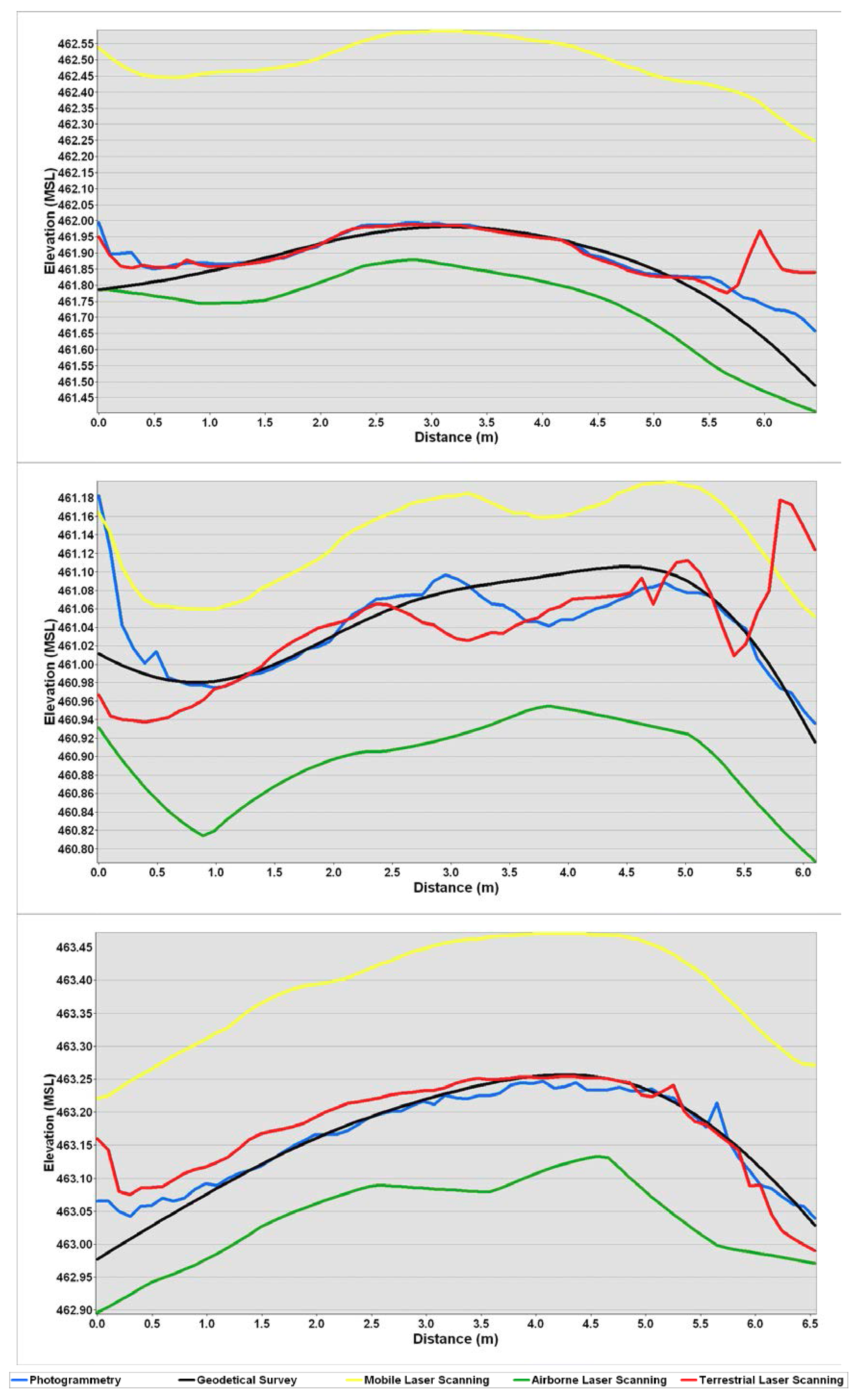
The preliminary data analysis showed that the MLS model had very large deviations in the order of up to tens of centimetres, especially in places with a closed canopy, which was affected by the quality of the GNSS signal. In the case of other models, significant deviations at the road shoulders up to 0.8 m were found (Figure 5). These deviations are caused by the low vegetation growth on the road shoulders. During the time of imaging, the vegetation was not removed; therefore, it was captured instead of the wearing course. This had an effect on the results shown in Table 2. Due to this, only the points with a distance greater than 1 m from the road edges were included in the final evaluation. This condition during evaluation does not influence the final precision of the models for the given purpose but only facilitated automatic elimination of vegetation on the road edges on both sides.
The statistical data set was reduced (from 404 to 206 points), but the accuracy of all models increased significantly (Table 3).
The calculated differences between the models and geodetic measurements are shown in Table 3. The smallest deviations and the highest height accuracy were achieved with the photogrammetric image processing method, where the RMSE was 0.011 m with a maximal deviation of 0.044 m. The TLS and the ALS methods reached RMSE 0.024 m with a maximum deviation of 0.088 m and RMSE 0.1392 m with a maximum deviation of 0.273 m, respectively. The worst results were achieved by MLS with an RMSE of 0.3167 m and a maximum deviation of −0.6579 m (Table 3). Figure 5 shows the best results of the photogrammetric data processing method, where the lowest error is clearly visible contrary to the highest error of the MLS method where the results are affected by the accuracy of GNSS under the canopy. At the same time, the vegetation effect on TLS and photogrammetry is seen at the edges.
4. Discussion
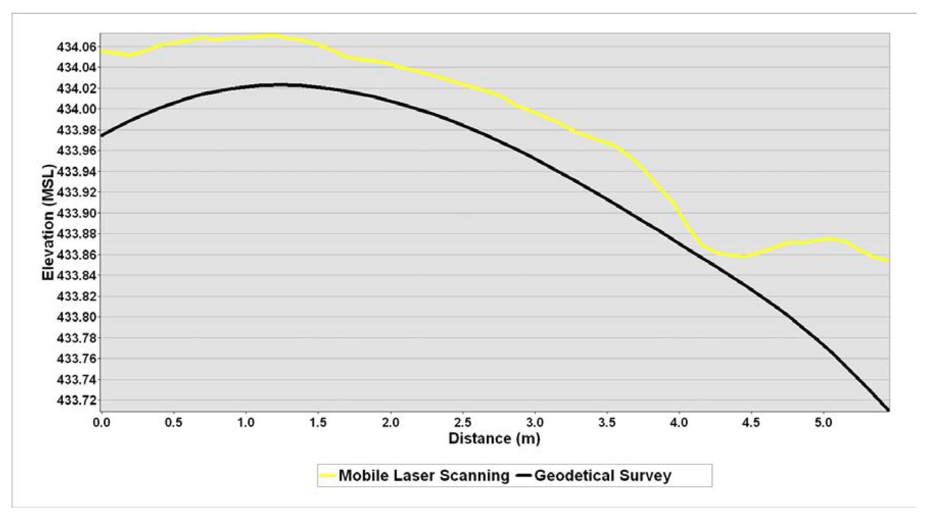
The results show that the method of mobile photogrammetry is very accurate but also allows imaging by commercially available cameras. The resulting point cloud reaches very high density even when a 12MP camera is used, due to the scanning height of about 1.5 m. Higher vertical accuracy of the model was achieved in comparison with other studies [66,67], where a 16-MP camera was used and the respective RMSE reached 0.0198 m and 0.0260 m. Large model errors at the road shoulders are caused by the technology itself because the point cloud is formed from a visible surface, i.e., including vegetation. However, this problem is reflected in all methods used, and therefore the data capture after the maintenance of the road is a prerequisite for the successful use of the methods. A high amount of ground control points (GCPs) surveyed either using GNSS or total station is required to create an accurate model. A lower amount of GCPs caused higher deviations from profiles surveyed by geodetic methods. The close range photogrammetric method also achieves the highest density of points per square meter, which is essential in practical use for the detailed calculation of road wearing course damage. This method is also independent of the car movement and possible vibrations while driving do not affect the final results. The SfM algorithm handles the images based on the current camera position and the basic condition is therefore only to obtain a good-quality image. The only condition for successful model creation is lower car speed due to optimum overlay of individual pictures. High-quality results achieved by the TLS method come from the scanner parameters and the used procedure where the individual scans were carried out, each about 40 m, to gain a sufficient overlap. The spacing between points within 10 m from the scanner was less than the 6 mm as mentioned in Section 2.3. Similar settings were used in Choi et al. [35], who noted that spacing between points within 10 m from the scanner was less than 5 mm. However, even with this setting, the resulting accuracy and point density are lower than in the case of the photogrammetry but much higher than in the case of the MLS. The registration of individual scans and the georeferencing are the important factors for the accuracy of the resulting surface model [39]. The georeferencing of the model in the coordinate system is done based on control points (located throughout the road) which also serve as points for alignment of the scans. The precision of these activities plays a very important role in accuracy evaluation of the used method. In this study, alignment including georeferencing was performed with a mean error of 0.0012 m and the maximum deviation was 0.0095 m. These values guarantee that TLS can provide very accurate information about the location and extent of wearing course damage. This is also confirmed by Valença [68], who pointed out that cracks in the wall of bridge pillars can be detected with 2 mm spatial resolution and scanner distance of 12.5 m from the object. There are also disadvantages in spite of all the advantages of this method. The main disadvantage is the lowest time efficiency: the method requires frequent transfer and placement (positioning) of the scanner [3]. Therefore, the method is inappropriate to map linear structures, but more suitable for targeting of local damage. Compared to the TLS, it is possible to survey even larger areas in a shorter time horizon [69]. However, there is a problem with the GNSS signal reception affected by forest closed canopy in the case of forest road mapping. Therefore, the method is well-suited for road survey outside forest stands, or control points should be measured for better georeferencing in forest areas. Results from places with forest canopy are significantly affected by the GNSS error and require further processing. The resulting MLS accuracy is also affected by the vehicle speed or the type of scanner used. Road scanning was performed at a speed of about 20 km/h, resulting in lower point cloud density (after filtration of 26 p/m2). However, the point density range is from 1 to 120 (pts/m2) after filtration. The point cloud covers not only the road but also its surroundings at nearly 80 m distance in both directions. On the road, the point density will be larger than 26 (pts/m2) because it is closer to the scanner. As we are interested only in the road, which is almost flat, a larger point density will not have a significant influence on the quality of the created DTM. Lim et al. [70] achieved a vertical accuracy of 0.053 m determined from the point cloud of mean density (128 p/m2) obtained at a vehicle speed of 8 km/h; the scanning angle also affects the density of the points in addition to the vehicle speed. Zhou and Vosselman [71] achieved similar accuracy (RMSE = 0.06 m) at a vehicle speed of between 30 and 40 km/h and with density of approximately 1000 p/m2. Previous studies show that the speed of the car does not affect the resulting accuracy of the model. In this case, the greater density despite the higher speed of the vehicle was given by the flat surface in the urban area. Therefore, it was not necessary to filter points of vegetation. Guan et al. [72] used 30 control points surveyed by GNSS to assess the accuracy of the MLS. The mean standard deviations of vertical accuracy for two laser scanners were 0.042 m and 0.033 m. In all of these cases, it is evident that the mean quadratic error in the vertical direction is very similar, ranging from 0.03 m to 0.06 m. This precision is sufficient for creation of a very accurate model of a road leading through an open space. To test the quality of the created model from the MLS, we also calculated the differences between 100 measured points and the part of our road (about 150 m) outside the forest. As we can see from the results presented in Table 4 and Figure 6, the RMSE is in full agreement with other published studies.
It could be stated that MLS is very precise technique for road inspection. Less accuracy in the MLS results would be caused by the lack of an absolute orientation under forest cover. As we can see from the results in Table 2 and Table 3, in the forest areas with a dense canopy, control points should be measured for better georeferencing of the trajectory, or, for example, to overcome the loss of a GNSS signal in the forest, Kukko et al. [57] used graph SLAM correction method (tree stem feature location) for correcting the post-processed GNSS-IMU trajectory for positional drift.
The ALS method showed an RMSE accuracy of 0.1392 m, which coincides with already published results [12,13,14]. Surprising is the increase of RMSE in the case of ALS after elimination of sideways. This phenomenon is due to a higher average error, which is probably due to a lower number of values and generally to an ALS error. The effect of vegetation on sideways could also be lower because the ALS was carried out during September when the vegetation on sideways had been cut. The ALS has very low point density and thus the created DTM has lower precision that is also influenced by interpolation of distant points. All these factors affect the accuracy of the final results. However, the method is hardly usable to determine the extent of damage and maintenance needed in individual forest roads. This all gives an impression of dual work for forest managers or planners and it can be one of the reasons why these methods have not been successfully implemented in practice.
In general, it can be stated that a higher point cloud density may affect the resulting detail of road damage, but it does not significantly affect the accuracy of the used methods. In addition to ALS, all methods achieve higher point densities than geodetic measurements where the points were measured at distances of 20 cm. Therefore, all cross profiles from geodetical survey are smoother than the others and eliminate local road roughness because they are affected by linear interpolation of distant points.
The wearing course of the running surface is usually constructed with a 4-cm thick bituminous layer. In the case of a breakdown, the underlying bearing base course layer of the road is further damaged, which has a significant effect on its lifetime. This also results in the necessary vertical accuracy of the presented methods up to 4 cm in height. This is only satisfied by the TLS and CRP used methods with respective RSME values of 0.0110 m and 0.0243 m taken at a distance of 1.5 m of the target. Practically, due to the mobility of the CRP method and the fact that the forest road is a linear construction, the CRP method is more convenient for this mapping.
5. Conclusions
3D Imaging represents a totally different approach to data acquisition and especially data processing. The time spent by conventional geodetic measurements in the field is transferred to data processing in the office. However, the data processing in the office is mostly automated using computer programs. This provides greater comfort for workers and greater independence from outdoor weather conditions. Moreover, the processing of the 3D model contributes to greater flexibility with regard to possible later changes and point position detection in any part of the model, which is not possible with the conventional geodetic measurement without returning to the terrain. It is related to the very positive results of the close range photogrammetry which uses affordable technical equipment and thus becomes available to a wide range of users. In the case of forest roads, the most important role is played by the precision achieved in the forest environment. The close range photogrammetry, in contrast to the terrestrial laser scanning, allows time-saving creation of a 3D model of lines. Further CRP research should focus on optimizing the amount and distance of GCPs and their influence on the final precision. It is also possible to examine data capture by means of a video that would allow a higher speed of the vehicle when collecting data. The design breakage of the wearing course is up to 25% of its area on forest roads. If the damage is greater, it is necessary to cover the running surface with the new wearing course. In the future, it will be also appropriate to verify the horizontal accuracy of the CRP method so that it is practically usable for determining the percentage of damage to the road surface.
Acknowledgments
Supported by the Specific University Research Fund of the FFWT Mendel University in Brno no. LDF_PSV_2016016 and project no. LO1408 “AdMaS UP—Advanced Materials, Structures and Technologies”, supported by Ministry of Education, Youth and Sports under the “National Sustainability Programme I”.
Author Contributions
P.H. initiated the study, carried out and reviewed the statistical analysis and the manuscript. T.M. conducted the GIS and statistical analysis and drafted the manuscript. N.T. and Z.K. carried out mobile laser scanning and processed the data. M.C. carried out terrestrial laser scanning and processed the data. A.P. carried out photogrammetry data and their processing and corrected the manuscript. Z.P. prepared the database and revised the manuscript.
Conflicts of Interest
The founding sponsors had no role in the design of the study; in the collection, analyses, or interpretation of data; in the writing of the manuscript, and in the decision to publish the results.
References
- Bogus, S.M.; Song, J.; Waggerman, R.; Lenke, L.R. Rank correlation method for evaluating manual pavement distress data variability. J. Infrastruct. Syst. 2010, 16, 66–72. [Google Scholar] [CrossRef]
- Abdie, E.; Sisakht, S.R.; Goushbor, L.; Soufi, H. Accuracy assessment of GPS and surveying technique in forest road mapping. Ann. For. Res. 2012, 55, 309–317. [Google Scholar]
- Rodriguez-Perez, J.R.; Alvarez, M.F.; Sanz-Ablanedo, E. Assessment of low-cost receiver accuracy and precision in forest environments. J. Surv. Eng. 2007, 133, 159–167. [Google Scholar] [CrossRef]
- Lehtomäki, M.; Jaakkola, A.; Hyyppä, J.; Kukko, A.; Kaartinen, H. Detection bogusof Vertical Pole-Like Objects in a Road Environment Using Vehicle-Based Laser Scanning Data. Remote Sens. 2010, 2, 641–664. [Google Scholar] [CrossRef]
- Li, Q.; Yao, M.; Yao, X.; Xu, B. A real-time 3D scanning system for pavement distortion inspection. Meas. Sci. Technol. 2009, 21. [Google Scholar] [CrossRef]
- Wang, K.C.P.; Gong, W.; Tracy, T.; Nguyen, V. Automated Survey of Pavement Distress Based on 2D and 3D Laser Images; The National Academies of Sciences, Engineering, and Medicine: Washington, DC, USA, 2011. [Google Scholar]
- Tsai, Y.J.; Li, F.; Wu, Y. A new rutting measurement method using emerging 3D line-laser-imaging system. Int. J. Pavement Res. Technol. 2013, 6, 667–672. [Google Scholar] [CrossRef]
- Azizi, Z.; Najafi, A.; Sadeghian, S. Forest Road Detection Using LiDAR Data. J. For. 2014, 25, 975–980. [Google Scholar] [CrossRef]
- Rowlands, A.; Sarris, A. Detection of exposed and subsurface archaeological remains using multi-sensor remote sensing. J. Archaeol. Sci. 2007, 34, 795–803. [Google Scholar] [CrossRef]
- Hyyppä, J.; Hyyppä, H.; Yu, X.; Kaartinen, H.; Kukko, A.; Holopainen, M. Forest Inventory Using Small-Footprint Airborne LiDAR. In Topographic Laser Ranging and Scanning, Principles and Processing; Shan, J., Toth, C.K., Eds.; CRC Press: Boca Raton, FL, USA, 2009. [Google Scholar] [CrossRef]
- Brenner, C. Building Reconstruction from Images and Laser Scanning. Int. J. Appl. Earth Obs. Geoinf. 2005, 6, 187–198. [Google Scholar] [CrossRef]
- Sithole, G.; Vosselman, G. Experimental Comparison of Filter Algorithms for Bare-Earth Extraction from Airborne Laser Scanning Point Clouds. ISPRS J. Photogramm. Remote Sens. 2004, 59, 85–101. [Google Scholar] [CrossRef]
- Hyyppä, J.; Hyyppä, H.; Litkey, P.; Yu, X.; Haggrén, H.; Rönnholm, P.; Pyysalo, U.; Pitkänen, J.; Maltamo, M. Algorithms and Methods of Airborne Laser Scanning for Forest Measurements; International Society for Photogrammetry and Remote Sensing (ISPRS): Freiburg, Germany, 2004; Volume XXXVI–8/W2, pp. 82–89. [Google Scholar]
- White, R.; Dietterick, B.C.; Mastin, T.; Strihman, R. Forest road mapped using LiDAR in steep forested terrain. Remote Sens. 2010, 2, 1120–1141. [Google Scholar] [CrossRef]
- Saito, M.; Goshima, M.; Aruga, K.; Matsue, K.; Shuin, Y.; Tasaka, T. Study of Automatic Forest Road Design Model Considering Shallow landslides with LiDAR Data of Funyu Experimental Forest. Croat. J. For. Eng. 2013, 34, 1–15. [Google Scholar]
- Aruga, K.; Sessions, J.; Miyata, E.S. Forest road design with soil sediment using a high-resolution DEM. J. For. Res. 2005, 10, 471–479. [Google Scholar] [CrossRef]
- Contreras, M.; Aracena, P.; Chung, W. Improving Accuracy in Earthwork Volume Estimation for Proposed Forest Roads Using a High-Resolution Digital Elevation Model. Croat. J. For. Eng. 2012, 33, 125–142. [Google Scholar]
- Aricak, B. Using remote sensing data to predict road fill areas affected by fill erosion with planned forest road construction. A case study in Kastamonu Regional Forest Directorate (Turkey). Environ. Monit. Assess. 2015, 187, 4663. [Google Scholar] [CrossRef] [PubMed]
- Dehvari, A.; Heck, J.H. Effect of LiDAR derived DEM resolution on terrain attributes, stream characterization and watershed delineation. Int. J. Agric. Crop Sci. 2013, 6, 946–967. [Google Scholar]
- Gallay, M.; Kaňuk, J.; Hochmuth, Z.; Meneely, J.D.; Hofierka, J.; Sedlák, V. Large-scale and high-resolution 3-D cave mapping by terrestrial laser scanning: A case study of the domica cave, Slovakia. Int. J. Speleol. 2015, 44, 277–291. [Google Scholar] [CrossRef]
- Wang, G.; Joyce, J.; Phillips, D.; Shrestha, R.; Carter, W. Delineating and defining the boundaries of an active landslide in the rainforest of Puerto Rico using a combination of airborne and terrestrial LIDAR data. Landslides 2013, 10, 503–513. [Google Scholar] [CrossRef]
- Barbarella, M.; Fiani, M. Monitoring of large landslides by terrestrial laser scanning techniques: Field data collection and processing. Eur. J. Remote Sens. 2013, 46, 126–151. [Google Scholar] [CrossRef]
- Dassot, M.; Constant, T.; Fournier, M. The use of terrestrial LiDAR technology in forest science: Application fields, benefits and challenges. Ann. For. Sci. 2011, 68, 959–974. [Google Scholar] [CrossRef]
- Marselis, S.M.; Yebra, M.; Jovanovic, T.; van Dijk, A.I.J.M. Deriving comprehensive forest structure information from mobile laser scanning observations using automated point cloud classification. Environ. Model. Softw. 2016, 82, 142–151. [Google Scholar] [CrossRef]
- Moskal, L.M.; Zheng, G. Retrieving forest inventory variables with terrestrial laser scanning (TLS) in urban heterogeneous forest. Remote Sens. 2011, 4, 1–20. [Google Scholar] [CrossRef]
- Tang, P.; Huber, D.; Akinci, B.; Lipman, R.; Lytle, A. Automatic reconstruction of as-built building information models from laser-scanned point clouds: A review of related techniques. Autom. Constr. 2010, 19, 829–843. [Google Scholar] [CrossRef]
- Shukor, S.A.A.; Wong, R.; Rushforth, E.; Basah, S.N.; Zakaria, A. 3D terrestrial laser scanner for managing existing building. J. Teknol. 2015, 76, 133–139. [Google Scholar] [CrossRef]
- Fais, S.; Cuccuru, F.; Ligas, P.; Casula, G.; Bianchi, M.G. Integrated ultrasonic, laser scanning and petrographical characterisation of carbonate building materials on an architectural structure of a historic building. Bull. Eng. Geol. Environ. 2017, 76, 71–84. [Google Scholar] [CrossRef]
- Hullo, J.F.; Thibault, G.; Boucheny, C. Advances in multi-sensor scanning and visualization of complex plants: The utmost case of a reactor building. ISPRS Arch. 2015, XL-5W4, 163–169. [Google Scholar] [CrossRef]
- Day, S.S.; Gran, K.B.; Belmont, P.; Wawrzyniec, T. Measuring bluff erosion part 1: Terrestrial laser scanning methods for change detection. Earth Surf. Process. Landf. 2013, 38, 1055–1067. [Google Scholar] [CrossRef]
- Ergincan, F.; Cabuk, A.; Avdan, U.; Tun, M. Advanced technologies for archaeological documentation: Patara case. Sci. Res. Essays 2010, 5, 2615–2629. [Google Scholar]
- Torres, J.A.; Hernandez-Lopez, D.; Gonzalez-Aguilera, D.; Moreno Hidalgo, M.A. A hybrid measurement approach for archaeological site modelling and monitoring: The case study of Mas D’Is, Penàguila. J. Archaeol. Sci. 2014, 50, 475–483. [Google Scholar] [CrossRef]
- Yastikli, N. Documentation of cultural heritage using digital photogrammetry and laser scanning. J. Cult. Heritage 2007, 8, 423–427. [Google Scholar] [CrossRef]
- Castagnetti, C.; Bertacchini, E.; Capra, A.; Dubbini, M. Terrestrial laser scanning for preserving cultural heritage: Analysis of geometric anomalies for ancient structures. In Proceedings of the FIG Working Week, Rome, Italy, 6–10 May 2012. [Google Scholar]
- Choi, M.; Kim, M.; Kim, G.; Kim, S.; Park, S.; Lee, S. 3D scanning technique for obtaining road surface and its applications. Int. J. Precis. Eng. Manuf. 2016, 18, 367–373. [Google Scholar] [CrossRef]
- Bitelli, G.; Simone, A.; Girardi, F.; Lantieri, C. Laser scanning on road pavements: A new approach for characterizing surface texture. Sensors 2012, 12, 9110–9128. [Google Scholar] [CrossRef] [PubMed]
- Přikryl, M.; Kutil, L. Consequences of a complex using of 3D approach in the implementation of the road reconstruction—Usage of TLS stop&go and usage of paving control system for milling machines. In Proceedings of the 6th International Conference on Engineering Surveying (INGEO 2014), Prague, Czech Republic, 3–4 April 2014. [Google Scholar]
- Barbarella, M.; De Blasiis, M.R.; Fiani, M.; Santoni, M. A LiDAR application for the study of taxiway surface evenness and slope. In ISPRS Annals Photogrammetry, Remote Sensing and Spatial Information Sciences, Proceedings of the ISPRS Technical Commision V Symposium, Riva del Garda, Italy, 23–25 June 2014; ISPRS: Göttingen, Germanny, 2014; Volume II-5. [Google Scholar] [CrossRef]
- Chin, A.; Olsen, M.J. Evaluation of technologies for road profile capture, analysis, and evaluation. J. Surv. Eng. 2015, 141. [Google Scholar] [CrossRef]
- Akgul, M.; Yurtseven, H.; Akburak, S.; Demir, M.; Cigizoglu, H.K.; Öztürk, T.; Eksi, M.; Akay, A.O. Short term monitoring of forest road pavement degradation using terrestrial laser scanning. Measurement 2017, 103, 283–293. [Google Scholar] [CrossRef]
- Wang, H. Development of Laser System to Measure Pavement Rutting. Master’s Thesis, University of South Florida, Tampa, FL, USA, 2005. Available online: http://digital.lib.usf.edu/SFS0025691/00001 (accessed on 7 November 2017).
- Demir, M.; Hasdemir, M. Functional planning criterion of forest road network systém according to recent forestry development and suggestion in Turkey. Am. J. Environ. Sci. 2005, 1, 22–28. [Google Scholar] [CrossRef]
- Mrics, S.W.; Clegg, P.; Jones, R. Combining terrestrial laser scanning, RTK GPS and 3D visualisation: Application of optical 3D measurement in geological exploration. In Proceedings of the 7th Conference on Optical 3D Measurement Techniques, Vienna, Austria, 3–5 October 2005. [Google Scholar]
- Jaakkola, A.; Hyyppä, J.; Hyyppä, H.; Kukko, A. Retrieval algorithms for road surface modelling using laser-based mobile mapping. Sensors 2008, 8, 5238–5249. [Google Scholar] [CrossRef] [PubMed]
- Bitenc, M.; Lindenbergh, R.; Khoshelham, K.; Van Waarden, A.P. Evaluation of a LiDAR land-based mobile mapping system for monitoring sandy coasts. Remote Sens. 2011, 3, 1472–1491. [Google Scholar] [CrossRef]
- Wang, J.; Gonzalez-Jorge, H.; Lindenbergh, R.; Arias-Sanchez, P.; Menenti, M. Geometric road runoff estimation from laser mobile mapping data. ISPRS Ann. Photogramm. Remote Sens. Spat. Inf. Sci. 2014, 2, 385–391. [Google Scholar] [CrossRef]
- Guan, H.; Li, J.; Cao, S.; Yu, Y. Use of mobile LiDAR in road information inventory: A review. Int. J. Image Data Fusion 2016, 7, 219–242. [Google Scholar] [CrossRef]
- Kumar, P.; Angelats, E. An automated road roughness detection from mobile laser scanning data. ISPRS Arch. 2017, 42, 91–96. [Google Scholar] [CrossRef]
- Böder, V.; Kersten, T.P.; Thies, T.; Sauer, A. Mobile laser scanning on board hydrographic survey vessels—Applications and accuracy investigations. In Proceedings of the FIG Working Week 2011, Marrakech, Morocco, 18–22 May 2011. Bridging the Gap between Cultures. [Google Scholar]
- Mitchell, T.; Suarez, G.; Chazaly, B. Evaluation of coastal vulnerability with mobile laser scanning from a vessel. In Proceedings of the IEEE Oceanic Engineering Society (OCEANS 2013), San Diego, CA, USA; 2013; pp. 1–5. [Google Scholar] [CrossRef]
- Szulwic, J.; Burdziakowski, P.; Janowski, A.; Kholodkov, A.; Matysik, K.; Matysik, M.; Przyborski, M.; Tysiąc, P.; Wojtowicz, A. Maritime Laser Scanning as the Source for Spatial Data. Pol. Marit. Res. 2015, 22, 9–14. [Google Scholar] [CrossRef]
- Yan, L.; Li, Z.; Liu, H.; Tan, J.; Zhao, S.; Chen, C. Detection and classification of pole-like road objects from mobile LiDAR data in motorway environment. Opt. Laser Technol. 2017, 97, 272–283. [Google Scholar] [CrossRef]
- Szulwic, J.; Tysiąc, P. Searching for road deformations using mobile laser scanning. MATEC Web Conf. 2017, 122. [Google Scholar] [CrossRef]
- Vallet, B.; Papelard, J.P. Road orthophoto/DTM generation from mobile laser csanning. ISPRS Ann. Photogramm. Remote Sens. Spat. Inf. Sci. 2015, II-3/W5, 377–384. [Google Scholar] [CrossRef]
- Kukko, A.; Kaartinen, H.; Hyyppä, J.; Chen, Y. Multiplatform approach to mobile laser scanning. ISPRS Arch 2012, XXXIX-B2, 483–488. [Google Scholar] [CrossRef]
- Pu, S.; Rutzinger, M.; Vosselman, G.; Elberink, S.O. Recognizing basic structures from mobile laser scanning data for road inventory studies. ISPRS J. Photogramm. Remote Sens. 2011, 66, 28–39. [Google Scholar] [CrossRef]
- Nurunnabi, A.; West, G.; Belton, D. Robust locally weighted regression for ground surface extraction in mobile laser scanning 3D data. ISPRS Ann. Photogramm. Remote Sens. Spat. Inf. Sci. 2013, 1, 217–222. [Google Scholar] [CrossRef]
- Kukko, A.; Kaijaluoto, R.; Kaartinen, H.; Jaakkola, A.; Hyyppä, J. Graph SLAM correction for single scanner MLS forest data under boreal forest canopy. ISPRS J. Photogramm. Remote Sens. 2017, 132, 199–209. [Google Scholar] [CrossRef]
- Kraus, K.; Pfeifer, N. Determination of terrain models in wooded areas with airborne laser scanner data. ISPRS J. Photogramm. Remote Sens. 1998, 53, 193–203. [Google Scholar] [CrossRef]
- Briese, C.; Pfeifer, N.; Dorninger, P. Applications of the robust interpolation for DTM determination. ISPRS Arch. 2002, 34, 55–61. [Google Scholar]
- Tyagur, N.; Hollaus, M. Digital terrain models from mobile laser scanning data in Moravian karst. ISPRS Arch. 2016, XLI-B3, 387–394. [Google Scholar] [CrossRef]
- Mandlburger, G.; Otepka, J.; Karel, W.; Wagner, W.; Pfeifer, N. Orientation and processing of airborne laser scanning data (OPALS)—Concept and first results of a comprehensive ALS software. ISPRS Arch. 2009, XXXVIII, 55–60. [Google Scholar]
- Otepka, J.; Mandlburger, G.; Karel, W. The OPALS Data Manager—Efficient Data Management for Processing Large Airborne Laser Scanning Projects. ISPRS Ann. Photogramm. Remote Sens. Spat. Inf. Sci. 2012, 1–3, 153–159. [Google Scholar] [CrossRef]
- Pfeifer, N.; Mandlburger, G.; Otepka, J.; Karel, W. OPALS–A framework for Airborne Laser Scanning data analysis. Comput. Environ. Urban Syst. 2014, 45, 125–136. [Google Scholar] [CrossRef]
- Ullman, S. The interpretation of structure from motion. Proc. R. Soc. Lond. Ser. B 1979, 203, 405–426. [Google Scholar] [CrossRef]
- Hrůza, P.; Mikita, T.; Janata, P. Monitoring of forest hauling roads wearing course damage using unmanned aerial systems. Acta Univ. Agric. Silvic. Mendelianae Brun. 2016, 64, 1537–1546. [Google Scholar] [CrossRef]
- Hrůza, P.; Mikita, T.; Janata, P.; Cibulka, M.; Patočka, Z. Accuracy of terrestrial imaging for the detection of forest road wearing course damage. Zpr. Lesnického Výzkumu 2017, 62, 75–81. [Google Scholar]
- Valença, J.; Puente, I.; Júlio, E.; González-Jorge, H.; Arias-Sánchez, P. Assessment of crack on concrete bridges using image processing supported by laser scanning survey. Constr. Build. Mater. 2017, 146, 668–678. [Google Scholar] [CrossRef]
- Liang, X.; Kankare, V.; Hyyppä, J.; Wang, Y.; Kukko, A.; Haggrén, H.; Yu, X.; Kaartinen, H.; Jaakkola, A.; Guan, F.; et al. Terrestrial laser scanning in forest inventories. ISPRS J. Photogramm. Remote Sens. 2016, 115, 63–77. [Google Scholar] [CrossRef]
- Lim, S.; Thatcher, C.A.; Brock, J.C.; Kimbrow, D.R.; Danielson, J.J.; Reynolds, B.J. Accuracy assessment of a mobile terrestrial lidar survey at Padre Island National Seashore. Int. J. Remote Sens. 2013, 34, 6355–6366. [Google Scholar] [CrossRef]
- Zhou, L.; Vosselman, G. Mapping curbstones in airbone and mobile laser scanning data. Int. J. Appl. Earth Obs. Geoinf. 2012, 18, 293–304. [Google Scholar] [CrossRef]
- Guan, H.; Li, J.; Yu, Y. 3D urban mapping using a Trimble MX8 mobile laser scanning system: A validation study. In Proceedings of the 8th International Symposium on Mobile Mapping Technology (MMT 2013), Tainan, Taiwan, 1–3 May 2013. [Google Scholar]
Figure 1.
The study area—forest road “Hradska” with cross profiles.
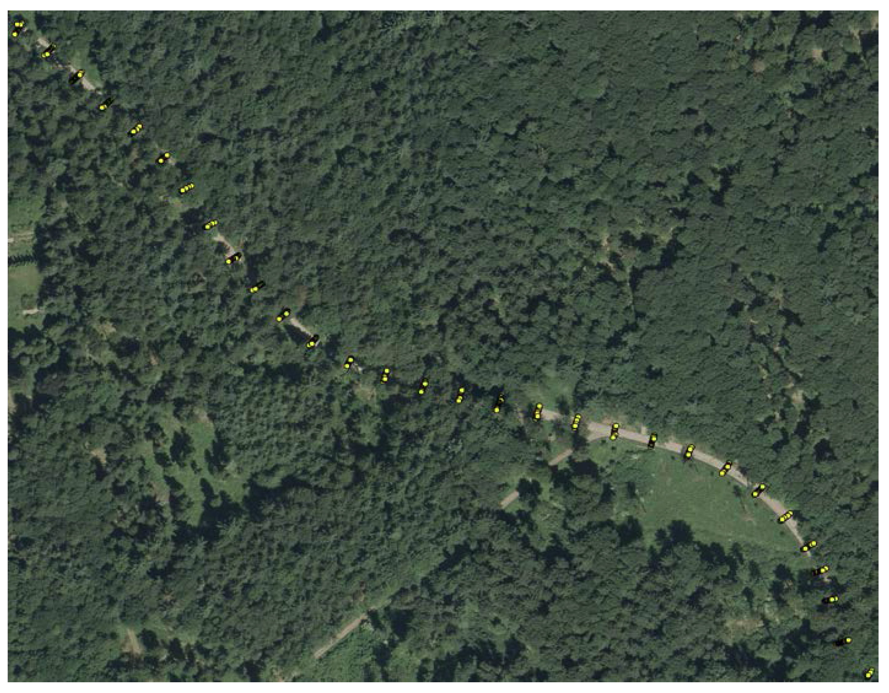
Figure 2.
Camera mount system on a car.

Figure 3.
Photogrammetric point cloud with cross profiles.

Figure 4.
Mobile laser scanning system Riegl VMX-450 mounted on a car.
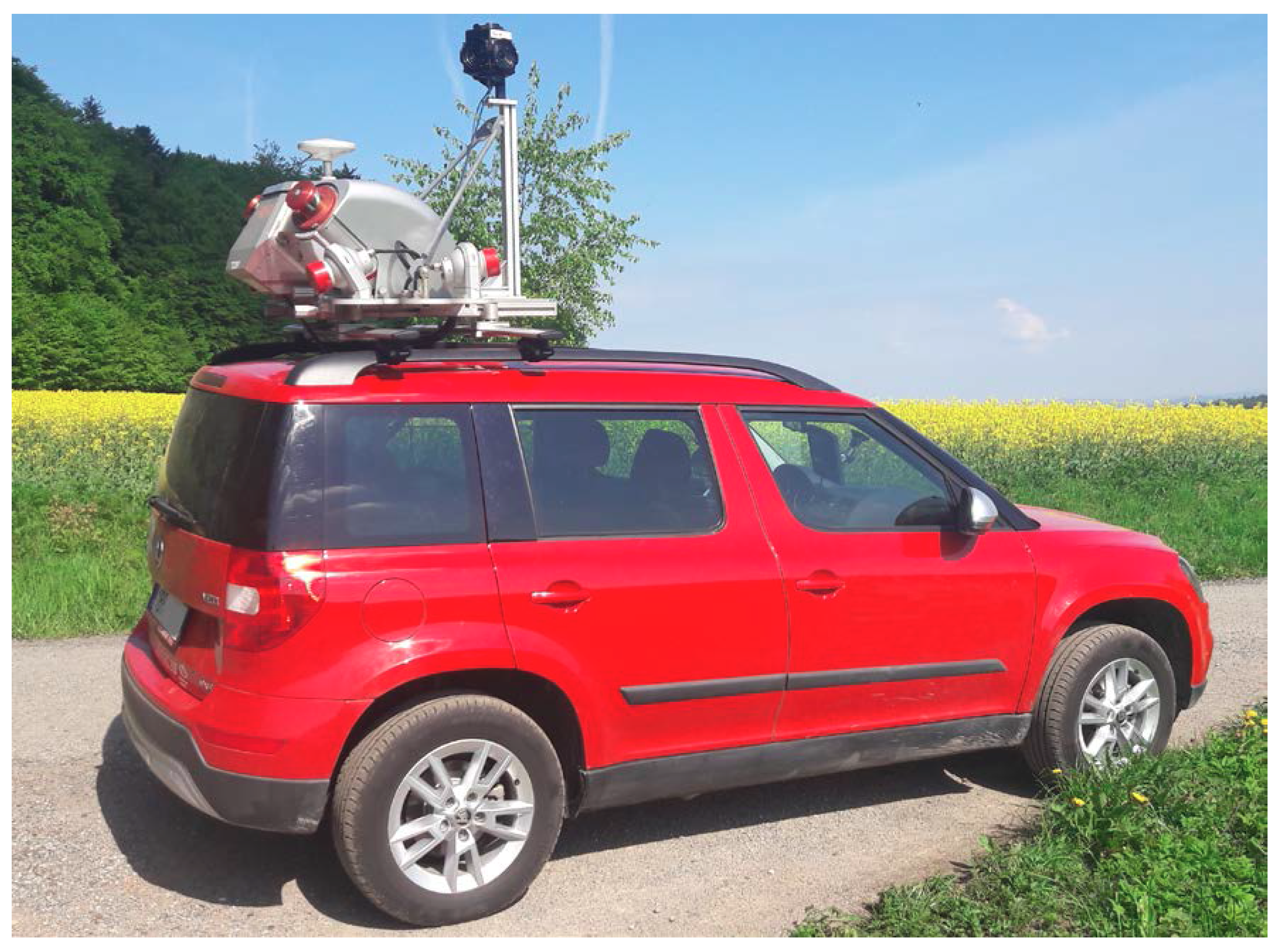
Figure 5.
Cross profile examples—comparison of different data sources.

Figure 6.
Example of cross profile outside of the forest stand.

Table 1.
Density of point clouds on road wearing course from different methods.
| Method | Point Cloud Density (pts/m2) |
|---|---|
| MLS | 26 |
| TLS | 17,882 |
| Photogrammetry | 18,276 |
| ALS | 1.13 |
Table 2.
Statistical evaluation of created models—vertical differences in metres before postprocessing.
Table 2.
Statistical evaluation of created models—vertical differences in metres before postprocessing.
| Method | Mean | Max | Min | Std. Dev. | RMSE |
|---|---|---|---|---|---|
| Mobile laser scanning | −0.2517 | 0.0049 | −0.8459 | 0.2014 | 0.4228 |
| Terrestrial laser scanning | −0.0396 | 0.1160 | −0.8930 | 0.1254 | 0.1315 |
| Photogrammetry | −0.0259 | 0.0400 | −0.4389 | 0.0605 | 0.0658 |
| Airborne laser scanning | 0.1130 | 0.3539 | −0.1469 | 0.0662 | 0.1309 |
Table 3.
Statistical evaluation of created models—vertical differences in metres after elimination of sideways.
Table 3.
Statistical evaluation of created models—vertical differences in metres after elimination of sideways.
| Method | Mean | Max | Min | Std. Dev. | RMSE |
|---|---|---|---|---|---|
| Mobile laser scanning | −0.2421 | 0.0040 | −0.6579 | 0.2042 | 0.3167 |
| Terrestrial laser scanning | 0.0011 | 0.0880 | −0.0701 | 0.0243 | 0.0243 |
| Photogrammetry | −0.0005 | 0.0242 | −0.0438 | 0.0110 | 0.0110 |
| Airborne laser scanning | 0.1320 | 0.2773 | 0.0159 | 0.0442 | 0.1392 |
Table 4.
Statistical evaluation of created model from MLS outside the forest—vertical differences in metres.
Table 4.
Statistical evaluation of created model from MLS outside the forest—vertical differences in metres.
| Method | Mean | Max | Min | Std. Dev. | RMSE |
|---|---|---|---|---|---|
| Mobile laser scanning | −0.0501 | 0.0049 | −0.1159 | 0.0273 | 0.0570 |
© 2018 by the authors. Licensee MDPI, Basel, Switzerland. This article is an open access article distributed under the terms and conditions of the Creative Commons Attribution (CC BY) license (http://creativecommons.org/licenses/by/4.0/).
Share and Cite
MDPI and ACS Style
Hrůza, P.; Mikita, T.; Tyagur, N.; Krejza, Z.; Cibulka, M.; Procházková, A.; Patočka, Z. Detecting Forest Road Wearing Course Damage Using Different Methods of Remote Sensing. Remote Sens. 2018, 10, 492. https://doi.org/10.3390/rs10040492
AMA Style
Hrůza P, Mikita T, Tyagur N, Krejza Z, Cibulka M, Procházková A, Patočka Z. Detecting Forest Road Wearing Course Damage Using Different Methods of Remote Sensing. Remote Sensing. 2018; 10(4):492. https://doi.org/10.3390/rs10040492
Chicago/Turabian StyleHrůza, Petr, Tomáš Mikita, Nataliya Tyagur, Zdenek Krejza, Miloš Cibulka, Andrea Procházková, and Zdeněk Patočka. 2018. "Detecting Forest Road Wearing Course Damage Using Different Methods of Remote Sensing" Remote Sensing 10, no. 4: 492. https://doi.org/10.3390/rs10040492
Note that from the first issue of 2016, this journal uses article numbers instead of page numbers. See further details here.