A New Strategy for Extracting ENSO Related Signals in the Troposphere and Lower Stratosphere from GNSS RO Specific Humidity Observations


1
School of Geodesy and Geomatics, Wuhan University, Wuhan 430079, China
2
Key Laboratory of Geospace Environment and Geodesy, Ministry of Education, Wuhan University, Wuhan 430079, China
*
Author to whom correspondence should be addressed.
Remote Sens. 2018, 10(4), 503; https://doi.org/10.3390/rs10040503
Submission received: 16 January 2018
/
Revised: 19 March 2018
/
Accepted: 20 March 2018
/
Published: 22 March 2018
(This article belongs to the Special Issue Multi-Constellation Global Navigation Satellite Systems: Methods and Applications)
Abstract
:El Niño-Southern Oscillation related signals (ENSORS) in the troposphere and lower stratosphere (TLS) are the prominent source of inter-annual variability in the weather and climate system of the Earth, and are especially important for monitoring El Niño-Southern Oscillation (ENSO). In order to reduce the influence of quasi-biennial oscillations and other unknown signals compared with the traditional empirical orthogonal functions (EOF) method, a new processing strategy involving fusion of a low-pass filter with an optimal filtering frequency (hereafter called the optimal low-pass filter) and EOF is proposed in this paper for the extraction of ENSORS in the TLS. Using this strategy, ENSORS in the TLS over different areas were extracted effectively from the specific humidity profiles provided by the Global Navigation Satellite System (GNSS) radio occultation (RO) of the Constellation Observing System for Meteorology, Ionosphere, and Climate (COSMIC) mission from June 2006 to June 2014. The spatial and temporal responses of the extracted ENSORS to ENSO at different altitudes in the TLS were analyzed. The results show that the most suitable areas for extracting ENSORS are over the areas of G25 (−25°S–25°N, 180°W–180°E) −G65(−65°S–65°N, 180°W–180°E) in the upper troposphere (250–200 hpa) which show a lag time of 3 months relative to the Oceanic Niño index (ONI). In the troposphere, ENSO manifests as a major inter-annual variation. The ENSORS extracted from the N3.4 (−5°S to 5°N, 120°W to 170°W) area are responsible for 83.59% of the variability of the total specific humidity anomaly (TSHA) at an altitude of 250 hpa. Over all other defined areas which contain the N3.4 areas, ENSORS also explain the major variability in TSHA. In the lower stratosphere, the extracted ENSORS present an unstable pattern at different altitudes because of the weak ENSO effect. Moreover, the spatial and temporal responses of ENSORS and ONI to ENSO across the globe are in good agreement. Over the areas with strong correlation between ENSORS and ONI, the larger the correlation coefficient is, the shorter the lag time between them. Furthermore, the ENSORS from zonal-mean specific humidity monthly anomalies at different altitudes can clearly present the vertical structure of ENSO in the troposphere. This study provides a new approach for monitoring ENSO events.
1. Introduction
El Niño-Southern Oscillation (ENSO), which originates in the tropical Pacific, is a natural, coupled ocean–atmospheric cycle with an approximate timescale of 2 to 7 years [1,2,3]. ENSO is a complicated system which has a profound effect, not only over the tropics, but also across the globe through teleconnections [3,4,5,6,7,8,9,10], and many aspects of its evolution are still not well understood [1]. Currently, the phases and strengths of ENSO events are quantified by indices corresponding to time, such as the equatorial tropical Pacific sea surface temperatures (SSTs) (e.g., Niño3.4 Index), and differences between the anomalies of a meteorological variable observed at two different stations (e.g., the Southern Oscillation Index (SOI)) [1,11]. Over the past two or three decades, the frequent occurrence of the ENSO phenomenon has attracted an upsurge in interest regarding the description and explanation of inter-annual fluctuations in weather and climate.
Investigating the El Niño-Southern Oscillation related signals (ENSORS) in the troposphere and lower stratosphere (TLS) and their response to ENSO are the subjects of many climate change detection studies [12,13]. Several researchers have studied ENSORS and analyzed their responses to ENSO events in the TLS. In the troposphere, a warming effect was observed during the warm phase of the ENSO cycle, and the maximum response to ENSO events occurred with a lag of one or two seasons [14,15,16,17,18,19]. In the lower stratosphere, a significant cooling signal was associated with El Niño events at low latitudes [20,21]. In contrast, a warming signal was found over the Artic stratosphere [21,22]. The transition between warming and cooling occurred across the tropopause during different ENSO events [13,16]. Most of the above-mentioned conclusions are associated with temperature signals obtained during ENSO events in the TLS. However, the response of TLS to different ENSO events on the basis of water vapor datasets has not been analyzed thoroughly.
Global Navigation Satellite System (GNSS) radio occultation (RO) datasets have the advantages of long-term stability, self-calibration, high accuracy, good vertical resolution, and all-weather global coverage. In recent years, GNSS RO measurements have proven useful for ENSO studies [13,17,23,24]. Lacker et al. [17] described ENSORS in the upper TLS region over the tropics using RO observations. Scherllin-Pirscher et al. [13] investigated the vertical and spatial structures of ENSORS, mainly over the tropical areas, by referring to RO temperature profiles and the total column water vapor variable derived from RO water vapor pressure. Teng et al. [23] characterized global precipitable water in ENSO events from 2007 to 2011 using datasets from the Constellation Observing System for Meteorology, Ionosphere, and Climate (COSMIC) mission. Sun et al. [24] illustrated the equatorial ENSORS at the tropopause observed by COSMIC from July 2006 to January 2012, and the COSMIC tropopause parameters were found to be useful for monitoring ENSO events. Although these studies described the vertical and spatial structures of atmospheric ENSORS over local regions, the phases and strengths of ENSO events were not fully determined. The temporal and spatial responses of the ENSORS in the TLS to ENSO were not clearly discussed. In addition, most of the studies were confined to tropical regions, and the impact of ENSO on a global scale needs further study.
ENSO is caused by complex interactions between the oceans and atmosphere, primarily through the transfer of heat and water vapor, and its evolution is highly related to variations in SST, wind, water vapor, and precipitation [25,26,27,28]. In the study of Lau et al. [26], approximately 80% of water vapor sensitivity to SST (i.e., deduced from ENSO anomalies) was caused by the transport of water vapor in large-scale circulation. Specific humidity is also a good indicator of ENSO because its value remains constant, even when large fluctuations exist in the temperature field—as long as moisture is not added to or reduced from a given mass (i.e., no phase change occurs) [29].
Identifying ENSORS in the TLS from specific humidity variability effectively is crucial, considering that the specific humidity variability in the TLS is not only affected by ENSO, but also by month-to-month variations, annual variations, quasi-biennial oscillation (QBO), as well as other unknown (unmodelled) factors (i.e., the fact that different underlying surfaces have different impacts on the lower troposphere and other factors beyond our current knowledge). Most of the previous studies have only used empirical orthogonal function (EOF) analysis to extract the ENSORS from the monthly anomalies of atmospheric parameters in the TLS [30,31]. However, the ENSORS extracted only by EOF may be artificially mixed with some residual noise or unknown (unmodelled) signals uncorrelated with ENSO [32] which could lead to uncertainties in the analyses [32,33]. In this work, a new strategy is brought forward, which is more stable in terms of specific humidity variability for the extraction of ENSORS in the TLS, compared with only using the EOF analysis. Under this strategy, considering that the annual and month-to-month variations have been eliminated from the monthly specific humidity anomalies, and in order to further eliminate QBO, other unrecognized signals and the residual noises of annual and month-to-month variations, the monthly anomalies of specific humidity are filtered by a low-pass filter with the optimal filtering cut-off frequency, before being processed by the EOF analysis. Using this strategy, ENSORS in the TLS are extracted from the GNSS RO specific humidity variability effectively, and the responses of the ENSORS to ENSO events in the TLS over different areas are explained quantitatively.
The main contributions and novelties in this study are as follows: (1) these ENSORS in the TLS are the first to be extracted from GNSS RO specific humidity profiles with this new strategy; (2) the spatial and temporal responses of ENSORS at different altitudes in the TLS are fully analyzed, and the most suitable areas and altitudes for extracting the ENSORS are found; (3) the vertical structure of ENSO in the troposphere is reconstructed with the GNSS RO specific humidity profiles.
2. Datasets and Methods
2.1. COSMIC GNSS RO Data
The data used in this study are specific humidity profiles retrieved from COSMIC GNSS RO for the period, June 2006–June 2014. The profiles are provided by the COSMIC Data Analysis and Archive Center (http://cosmicio.cosmic.ucar.edu/cdaac/index.html) of the University Corporation for Atmospheric Research. The COSMIC mission, which comprises a constellation of six micro low-earth-orbit (LEO) satellites at an altitude of 800-kilometers, was successfully launched on 15 April 2006 (see Rocken et al. [34] for details about the mission). The basic observations from GNSS RO measurements are comprised of GNSS radio signal phases between the LEOs and occulting GNSS satellite. Then, bending angles can be obtained from the signal phases. Finally, on the basis of the spherical symmetry assumption, refractivity can be derived from the bending angles [35,36]. In the neutral atmosphere, the atmospheric temperature , atmospheric pressure , and water vapor pressure are estimated by [37].
The recovery of or from measurements using the one-dimensional variational retrieval (1D-Var) method [38,39] requires temperature or water vapor data derived from the background model (e.g., ERA-Interim reanalysis). Specific humidity can be derived from , as expressed by Equation (2) [40].
where and and are the dry and moist air gas constants, respectively.
The COSMIC mission provided up to 2000 daily profiles with almost uniform global coverage and a horizontal resolution of around 300 km [23]. More than 90% of the profiles can penetrate the lowest 2 km of the troposphere by employing the “open-looping tracking” technique [23,41]. According to independent evaluations, the COSMIC GNSS RO specific humidity profiles in the TLS are sufficiently accurate for climate studies [41,42,43].
2.2. ENSO Indicators
To best define an ENSO event, the year of occurrence, strength, duration, and timing are considered [1]. Several different indices have been proposed for describing ENSO variability, such as the Niño1 + 2, Niño3, Niño4, and Niño3.4 (N3.4) indices. These indices were discussed in detail by Hanley [1]. The predictability of the N3.4 index is the highest among the indices. The N3.4 index was proven to be a good descriptor of ENSO [44], and several studies used the N3.4 index to represent ENSO events [45,46,47].
The Oceanic Niño index (ONI), which is defined by the three-month running mean SST anomaly in the N3.4 region (−5°S to 5°N, 120°W to 170°W), is available online from http://ggweather.com/enso/oni.htm. The National Oceanic and Atmospheric Administration (NOAA) uses ONI as the de facto standard for identifying El Niño (warm) and La Niña (cool) events in the tropical Pacific. The ONI defines an El Niño event as five consecutive overlapping three-month periods within or exceeding a anomaly and La Niña events within or below a anomaly in the N3.4 region. The events can be further categorized as weak (0.5–0.9), moderate (1.0–1.4), strong (1.5–1.9), and very strong (≥) SST anomalies, in which ONI equals or has exceeded the threshold for at least three consecutive overlapping three-month periods. In the present study, the ONI is used to represent ENSO signals.
2.3. Methodology
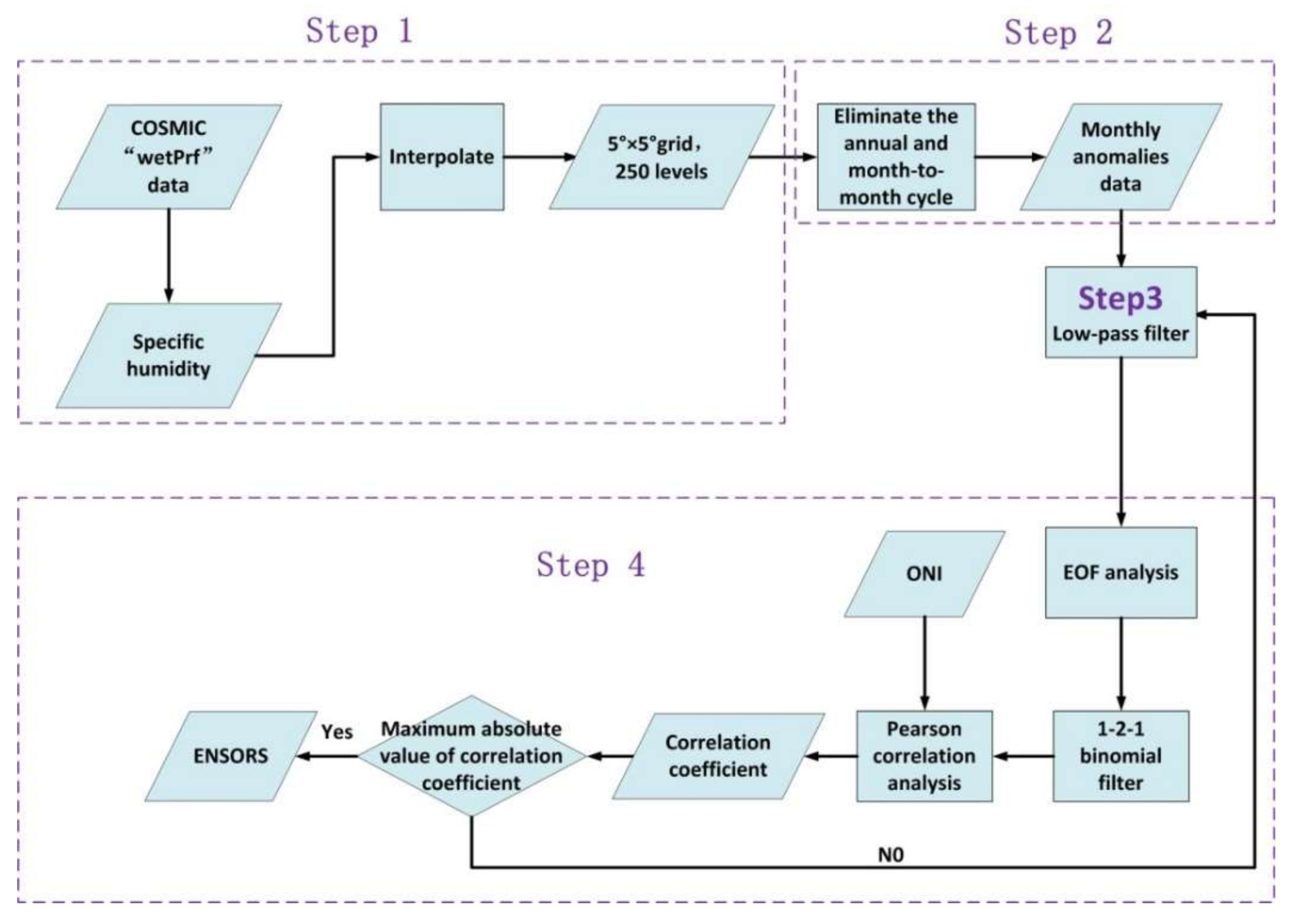
COSMIC GNSS RO specific humidity observations were employed to quantitatively understand the response to ENSO in the TLS for the period, June 2006–June 2014. The process of extracting the ENSORS in the TLS (see Figure 1) was as follows:
- (1)
- The original daily average data were interpolated into longitude–latitude grid points across the globe at different altitudes in the TLS using the nearest neighbor interpolation with inverse distance weighted method. Applying the method results in an Earth oblateness level error, but the error can be ignored. Owing to the relatively sparse distribution of COSMIC GNSS RO profiles over the polar region, the accuracy of the grid points in this region is lower than that of the other regions. Considering that the horizontal resolution of COSMIC observations is about , and to avoid the impact of tangent point horizontal drift (the drift from altitude 1 km to 10 km is about 102 km, and the drift from 1 km to 20 km is about 136 km [41]) of the COSMIC occultation point, a grid resolution of , which is slightly lower than the actual resolution of the occultation data, was adopted. The gridded specific humidity data are presented for 250 standard pressure levels (from 1000–100 hpa in 5 hpa steps, 100–30 hpa in 1 hpa steps) by linear interpolation from 1000 to 30 hpa (~0–25 km) in the vertical direction.
- (2)
- For each isobaric surface, the specific humidity monthly anomalies at each grid point were extracted through eliminating the annual and month-to-month variations in the monthly specific humidity time series at each point. The annual mean anomalies were obtained by subtracting the mean annual cycle (~372-day cycle) identified via fast Fourier transform at each grid point for the period, June 2006–June 2014. Then, the time series of monthly mean anomalies were obtained by taking the monthly average of the annual mean anomalies. The time series were then smoothed with a 1-2-1 binomial filter to reduce month-to-month variations [13,22].
- (3)
- For each isobaric surface, the monthly mean anomalies at each grid point were filtered by the low-pass filter with different filtering cut-off frequencies. Considering that the data length is 97 months for the period of June 2006–June 2014, the minimum cut-off frequency was set as 1/48.5 (assuming the maximum cycle of ENSORS is 48.5 months), the maximum cut-off frequency was set as 1, and so the cut-off frequency could be set to 1, 1/1.5, 1/2.0, ..., 1/48.5 (unit: 1/month). To determine the optimal cut-off frequency, we required a numerical low-pass filter to eliminate the high frequency signals. The frequency response, , of an ideal low-pass filter can be described by Formula (3).where is the cut-off frequency, and is the frequency of the signals of the monthly mean anomalies. Then, the corresponding impulse responses of an ideal low-pass filter, , obtained using the inverse Fourier transform method can be represented bywhere the time series, , at different cut-off frequencies can be obtained.
- (4)
- For each isobaric surface, the filtered time series of monthly mean anomalies () obtained from Step (3) were analyzed by EOF for all filtering cut-off frequencies. For each filtering cut-off frequency, the cross-correlation was carried out between the time series of EOF components and ONI. The optimal cut-off frequency of the low-pass filter was determined when the maximum absolute value of the correlation coefficient was obtained. The time series of EOF components which have the maximum absolute values of the correlation coefficient with the ONI were regarded as ENSORS.
The process of extracting the ENSORS in the TLS is shown in Figure 1.
In order to evaluate the effect of the optimal low-pass filter method, the absolute values of correlation coefficients between the ENSORS derived from the following two schemes and ONI were compared.
Scheme 1: The monthly mean anomalies of specific humidity from which the annual and month-to-month variations were subtracted were directly processed with EOF, which means that Step (3) in the process of extracting ENSORS is ignored in this scheme.
Scheme 2: The monthly mean anomalies of specific humidity from which the annual and month-to-month variations were subtracted were processed with the optimal low-pass filter and EOF. This is the complete process of the proposed method described above (Figure 1).
The compared results are discussed in Section 3.1. The results verify that the Scheme 2 is more suitable for extracting the ENSORS from the TLS (see next section). To determine the most suitable areas to extract ENSORS from, the globe was divided into 27 regions. The detailed definitions for the 27 regions are listed in Table 1.
In this study, we used the Pearson cross-correlation coefficient to describe the response strength to ENSO events in the TLS. The correlation coefficients in this work are all statistically significant with Student’s t-tests at the 95% confidence level [48].
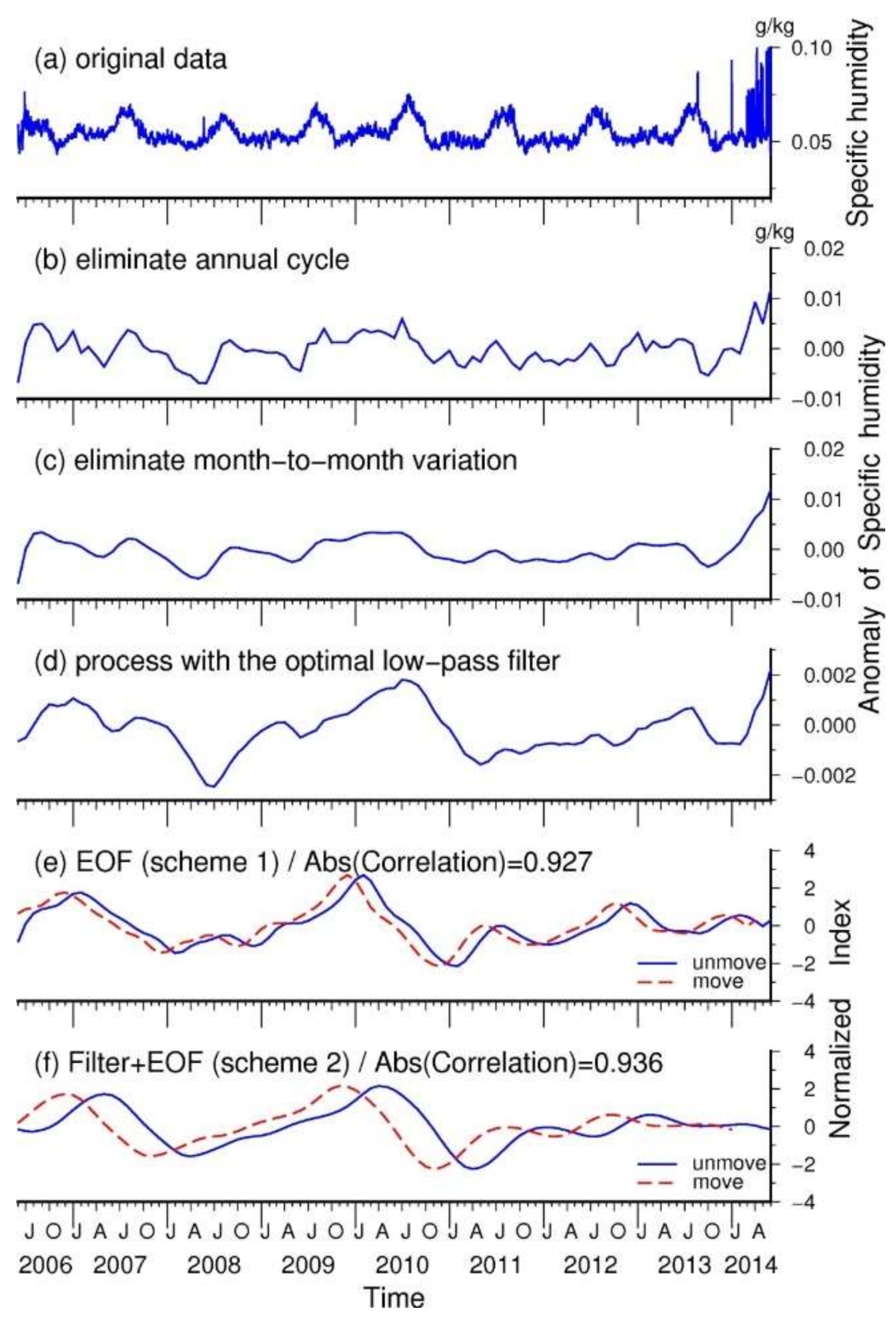
Figure 2 gives an example which clarifies the function of each step in the data processing procedure for extracting ENSORS. In this work, all grid data were processed with the proposed strategy to extract ENSORS. Hence, in this figure, we use the global averages of specific humidity as the original data at an altitude of 245 hpa. In addition, we have provided the step-by-step results, i.e., the monthly anomalies which have been eliminated the mean annual cycle, which have been further reduced the month-to-month variations by applying the 1-2-1 binomial filter, and which have been even further reduced other unknown factors and the residual signals from Step (2) in Figure 1 by applying the low-pass filter with the optimal cut-off frequency. The ENSORS were extracted either only by EOF (Scheme 1), or by low-pass filter and EOF (Scheme 2). The correlation coefficients in Figure 2e,f are statistically significant with Student’s t-tests at the 95% confidence level. The comparison between Figure 2e and Figure 2f shows that compared with Scheme 1, Scheme 2 improves the correlation coefficient between the extracted ENSORS and the ONI, although the correlation coefficient between the ENSORS and ONI extracted with Scheme 1 can also be up to 0.927 lagging the ONI by 2 months.
3. Results and Discussion
We extracted ENSORS from COSMIC GNSS RO specific humidity profiles using the two methods outlined in Section 2.3. Then, we analyzed the response of the ENSORS to ENSO over different areas and identified the suitable areas and altitudes to extract ENSORS in the TLS. Finally, the spatial and vertical structures of ENSO were investigated with the proposed method in the TLS.
3.1. Extracting ENSORS in the TLS
The ENSORS over different areas (Table 1) were extracted by the proposed method (the optimal low-pass filter + EOF, Scheme 2) and only by EOF (Scheme 1) in the TLS, respectively. The maximum lead/lag time was set as 24 months. Given that ONI is used to represent ENSO signals, we analyzed the ENSORS extracted from the areas that contain the N3.4 area by the two methods and compared them with the ONI in the TLS.
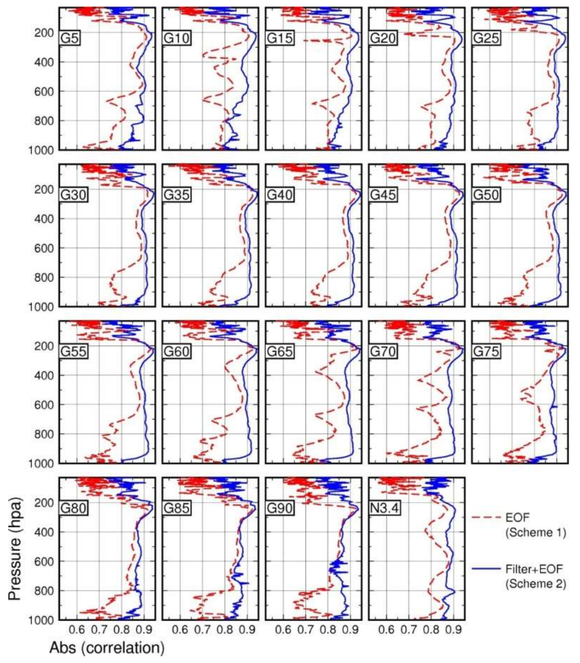
In this work, we define the intensity of the response to ENSO with the absolute values of the correlation coefficient between the extracted ENSORS and ONI. Figure 3 depicts the absolute value of the correlation coefficient between ENSORS and ONI at each isobaric pressure altitude in TLS. It can be seen that the absolute values of the correlation coefficients between ENSORS and ONI based on Scheme 2 are significantly higher than those based on Scheme 1 for all statistical areas in the TLS, especially in the lower stratosphere and lower troposphere. Therefore, we choose Scheme 2 to analyze the response to ENSO in the TLS. In addition, the ENSORS derived from the G25-G65 areas with the proposed method (Scheme 2) presented similar patterns in the TLS. The stability when extracting the ENSORS and the strongest response to ENSO at different altitudes in the TLS are analyzed in Section 3.2.
3.2. Response to ENSO in the TLS
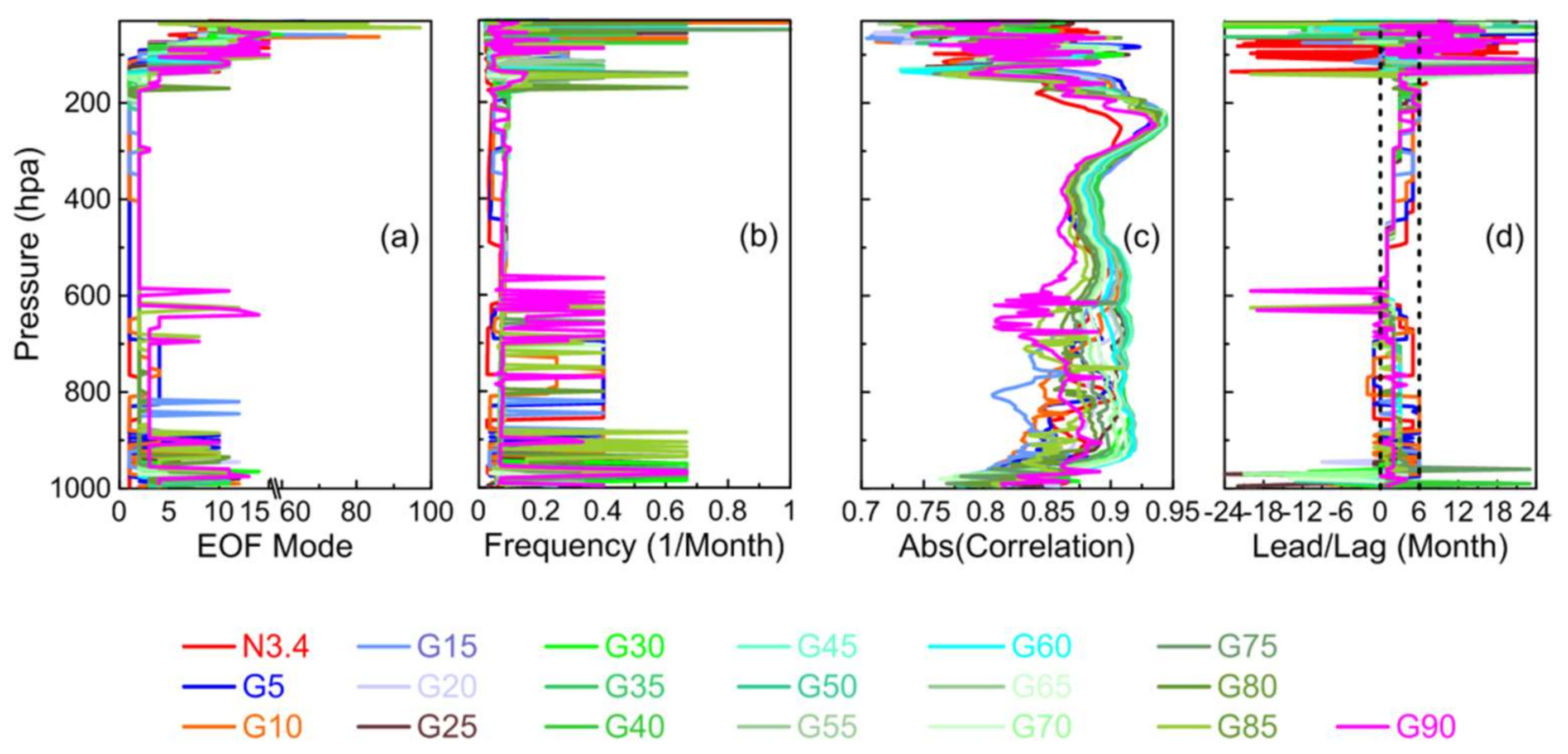
In the TLS, the impacts of other different factors, such as QBO, in the upper troposphere and lower stratosphere, the effect of different underlying surfaces over different regions, and other unknown factors at different altitudes, may exist in the time series of monthly mean anomalies of specific humidity at different altitudes. Although these mixed factors cannot be recognized and be separated completely, the differences in these mixed factors at different altitudes are reflected by the EOF modes and the filtering frequencies of the optimal low-pass filter. At different altitudes, the corresponding EOF time modes that have the maximum absolute values of correlation coefficients between EOF time modes (ENSORS) and ONI are not necessarily the same. For a certain height range, if the chosen EOF mode stays almost unchanged at different altitudes, we consider that the ENSORS can be extracted stably over this height range. Consequently, the curves of the absolute correlation coefficient values between the extracted ENSORS and ONI are smooth, and the lead/lag times and the cut-off frequencies also remain almost unchanged at different altitudes over this height range. Thus, we selected two variables—the EOF mode and the filtering frequency of the optimal low-pass filter—to analyze the stability when extracting ENSORS in the TLS (Figure 4a,b).
As shown in Figure 4, the ENSORS are stable in the middle and upper troposphere (~560 to ~150 hpa) but not very stable in the lower troposphere and lower stratosphere regions. Due to being situated near the underlying surface, lower tropospheric convection is very intense. Water vapor in the lower troposphere is affected by other unknown factors besides the ENSO phenomenon, as shown by the different EOF modes at different altitudes in Figure 4a and the different filtering frequencies at different altitudes in Figure 4b. The EOF mode is neither the first mode nor the second one, and the EOF modes change dramatically (<560 hpa) over several areas, especially near the surface (Figure 4a). The filtering frequencies also vary greatly at different altitudes under 560 hpa (Figure 4b). As shown in Figure 4b, the filtering frequencies under 560 hpa are larger than 0.4 (2.5 months) and increase to as high as 0.6 (1.6 months) near the Earth’s surface. The results indicate that the ENSO is not the only factor which influences the monthly anomalies in specific humidity in the lower troposphere. In the lower stratosphere, the QBO dominates the inter-annual variations, and the ENSO effect is weak [18,21,22]. Thus, the maximum absolute values of the correlation coefficients in the lower stratosphere (>0.7) are less than those in the troposphere (>0.8). Moreover, the EOF modes are large and the filtering frequencies are unstable at different altitudes in the lower stratosphere. With regard to the temporal response to ENSO in the lower stratosphere, the extracted ENSORS do not present similar patterns at different altitudes. For a range of altitudes, the ONI is delayed by several months, while for other altitudes, the ONI is advanced by several months, some even by more than 24 months. As shown in Figure 4d, the lag time of the ENSORS corresponding to the ONI in the troposphere is 0–6 months (2 seasons), which is consistent with previous results based on temperature profiles [13,16,19]. Figure 4c shows that for certain altitudes in the TLS, the absolute values of the correlation coefficients between the extracted ENSORS and ONI do not vary much over the 19 areas defined here, especially in the middle and upper troposphere (~560 to ~150 hpa). The maximum values are observed over the areas, G25–G65. These results verify that although ENSO originates from the tropical Pacific, the area with the strongest response to ENSO extends to G25–G65. The peak values are attained in the upper troposphere (250–200 hpa) with a lag time of 3–6 months (2 seasons), as shown by Figure 4c,d. The maximum values can be greater than 0.94 in the upper troposphere over some altitudes. As depicted in Table 2, the absolute values over different areas at different altitudes in the TLS might reach the maximum when the extracted ENSORS delay ONI by 3–6 months. The corresponding EOF modes over different areas are the first modes (N3.4, G5, G10, and G15) or the second modes (G20–G90). Over the N3.4 area, the first EOF mode accounts for 82.59% of the monthly anomaly variance in the specific humidity. With the expansion of the region, the percentage of the variance explained by the corresponding EOF modes decreases gradually over different areas, except for G90 areas (10.03%) (Table 2). Thus, these results further confirm that ENSO is the most important source of inter-annual variation over low-latitude areas in the troposphere. ENSO can also explain the major variations in the total specific humidity anomaly (TSHA) over other areas which contain the N3.4 area. Besides, the maximum absolute values are all found in the upper troposphere.
As is noted in Section 3.1, the areas over G25–G65 presented similar patterns in the TLS. As shown in Table 2, the EOF mode, the filtering frequency and the lag time of ENSO all tend to be stable when the absolute values of correlation coefficients between the extracting ENSORS and ONI reach a maximum. Therefore, to further analyze the results of Figure 4, the ENSORS extracted from the areas (G25–G65) are depicted in Figure 5. The extracted signals, which are very stable over the altitudes of 940–150 hpa over the G25 area, are similar to those over the G30–G65 areas (Figure 5). These results indicate that across all of the G25–G65 areas, the monthly anomalies in the specific humidity for altitudes of 940–150 hpa are affected by similar factors. The strongest responses to ENSO were found at altitudes of 250–200 hpa with a lag of 3 months (Table 2).
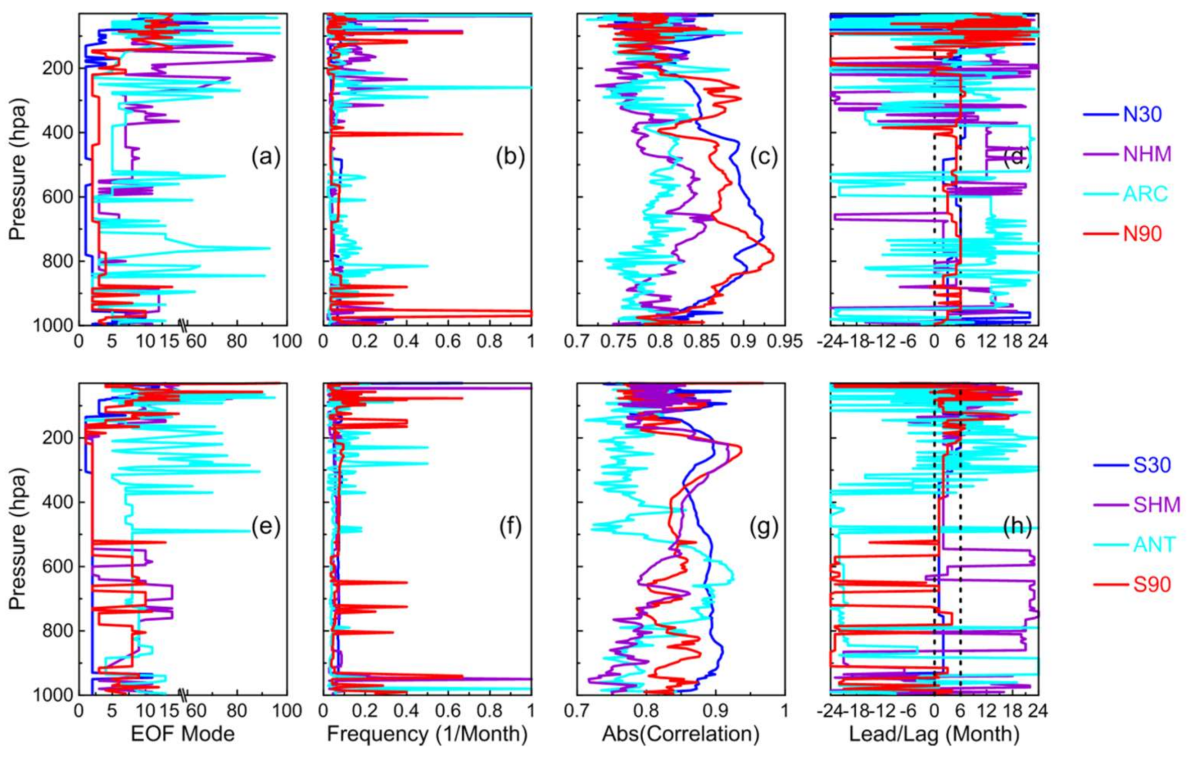
In order to study the influence of ENSO over other areas (i.e., excluding N3.4), we extracted ENSORS from the areas of N30, NHM, ARC, N90, S30, SHM, ANT, and S90 (Figure 6). The ENSORS of these eight areas differ from those of the N3.4 area at different altitudes. The maximum absolute values of the correlation coefficients between the ENSORS derived from these areas and ONI can be greater than 0.93 (Table 3). These results indicate the global effect of ENSO. We can further extract ENSORS from the specific humidity in the TLS over any geographical area. In Figure 6, the response time, the corresponding EOF modes, and the filtering frequency are shown to be very unstable in the TLS, especially over the NHM, ARC, SHM, and ANT areas. Thus, these eight areas, excluding the N3.4 area, are not the most suitable areas for extracting ENSORS in the TLS. From Table 3, the variances in the EOFs are greater than 21% over the N30 and SHM areas and become very small over the NHM, ARC and ANT areas, indicating that ENSO has a significant effect over the N30 and SHM areas.
After extracting the ENSORS in the TLS, the time series of ENSORS were compared with the ONI. The time series of ENSORS at each isobaric surface were standardized as , where is the standardized time series, is the ENSORS time series, is the average of the extracted time series, and is the standard deviation of on the same scale. Figure 7 depicts the extracted ENSORS after moving forward a certain number of months (3–6 months) (i.e., see list in Table 2) over different areas during the period of June 2006–June 2014. The extracted ENSORS and ONI show similar inter-annual variability after moving forward 3–6 months over different areas (Figure 7). The absolute values of the correlation coefficients between ENSORS extracted from the G20–G65 areas and ONI reach the maximum (~0.94) after a delay of three months. Meanwhile, the absolute value of the correlation coefficient (~0.908) becomes the smallest after a delay of five months over the N3.4 area. The results verify that, in the TLS, the strongest response area is not the N3.4 area, which is because the ENSO signal has propagated into the atmosphere of middle and high latitudes by means of planetary Rossby waves and the meridional circulation (Table 2) [22].
Building on the above analysis, the G25–G65 areas are the most suitable for extracting ENSORS from the upper troposphere (250–200 hpa) with a lag time of 3 months using Scheme 2. The ENSORS extracted from these altitudes over these areas and ONI are highly correlated. The correlation coefficient can reach up to more than 0.94, which is far greater than the results given by Sun et al. [24], who analyzed the correlation coefficients of the time series of tropopause parameters (e.g., the height, pressure, temperature and potential temperature of the tropopause) derived from COSMIC over the N3.4 area and ONI. In their work, QBO and other unknown factors were not eliminated from these time series of tropopause parameters. Other than the tropopause, the results of this work indicate that the time series of ENSORS extracted from GNSS RO specific humidity with the proposed method can provide us with an opportunity to describe the phases and strengths of ENSO events in the upper troposphere.
3.3. Response to ENSO at an Altitude of 245 hpa across the Globe
Only by finding the altitudes with the strongest ENSO responses in the TLS can the spatial and temporal responses to ENSO in the atmosphere be adequately described. In Section 3.2, we established that the strongest response to ENSO across the globe was situated at the 245 hpa level, lagging the ONI by 5 months (Table 2). At the 245 hpa level, the maximum value of the correlation coefficient can reach up to 0.936. The ENSORS extracted from the globe are in the opposite phase to ONI. The extracted ENSORS over the globe, after moving forward 5 months, show similar inter-annual variability with ONI (Figure 7). To analyze the spatial and temporal responses to ENSO across the globe, the optimal low-pass filtering and EOF analysis methods were employed to extract ENSORS at an altitude of 245 hpa. Figure 8 depicts the maximum correlation coefficients between ENSORS and ONI across the globe and the corresponding lag/lead times over different areas at the 245 hpa level in the troposphere. As shown in Figure 8a,b, the spatial and temporal responses of ONI and the extracted ENSORS across the globe are in good agreement. The strongest correlations with ENSO were mainly concentrated over the G30 area. Positive responses were observed over east Africa, the equatorial Indian Ocean, and the central and Eastern tropical Pacific. In contrast, negative responses were found over the Western Pacific, coastal countries of South America, and the equatorial Atlantic Ocean. The negative correlations were also found at the 20–40° latitudes over both hemispheres. The spatial response patterns are presented in Figure 8a,c. These patterns are similar to corresponding results derived from the literature [44], which describe the correlations between SST and ONI. The corresponding temporal responses of ONI and ENSORS are presented in Figure 8b,d. Over these strongly correlated areas, delayed responses to ONI are also observed (Figure 8b). The patterns indicate that the larger the correlation coefficient, the shorter the lag time will be. Over the mid-latitudes (20–60°) of the Southern hemisphere, north of Australia, Colombia, Venezuela, Ecuador, and Peru’s Western waters, Brazil’s Northeastern waters, and other regions, the temporal responses relative to the ONI present early responses by approximately 1–2 years.
3.4. Specific Humidity Response to ENSO in the Vertical Direction
Previous studies [13,16,18] proposed using the zonal-mean temperature components in the TLS for the analysis of different ENSO signals. This study adopted the same approach to analyze the vertical structure derived from the GNSS RO specific humidity, and then investigated the specific humidity response to ENSO in the vertical direction. This section, describes the ENSORS extracted from zonal-mean specific humidity components in the TLS by the proposed method.
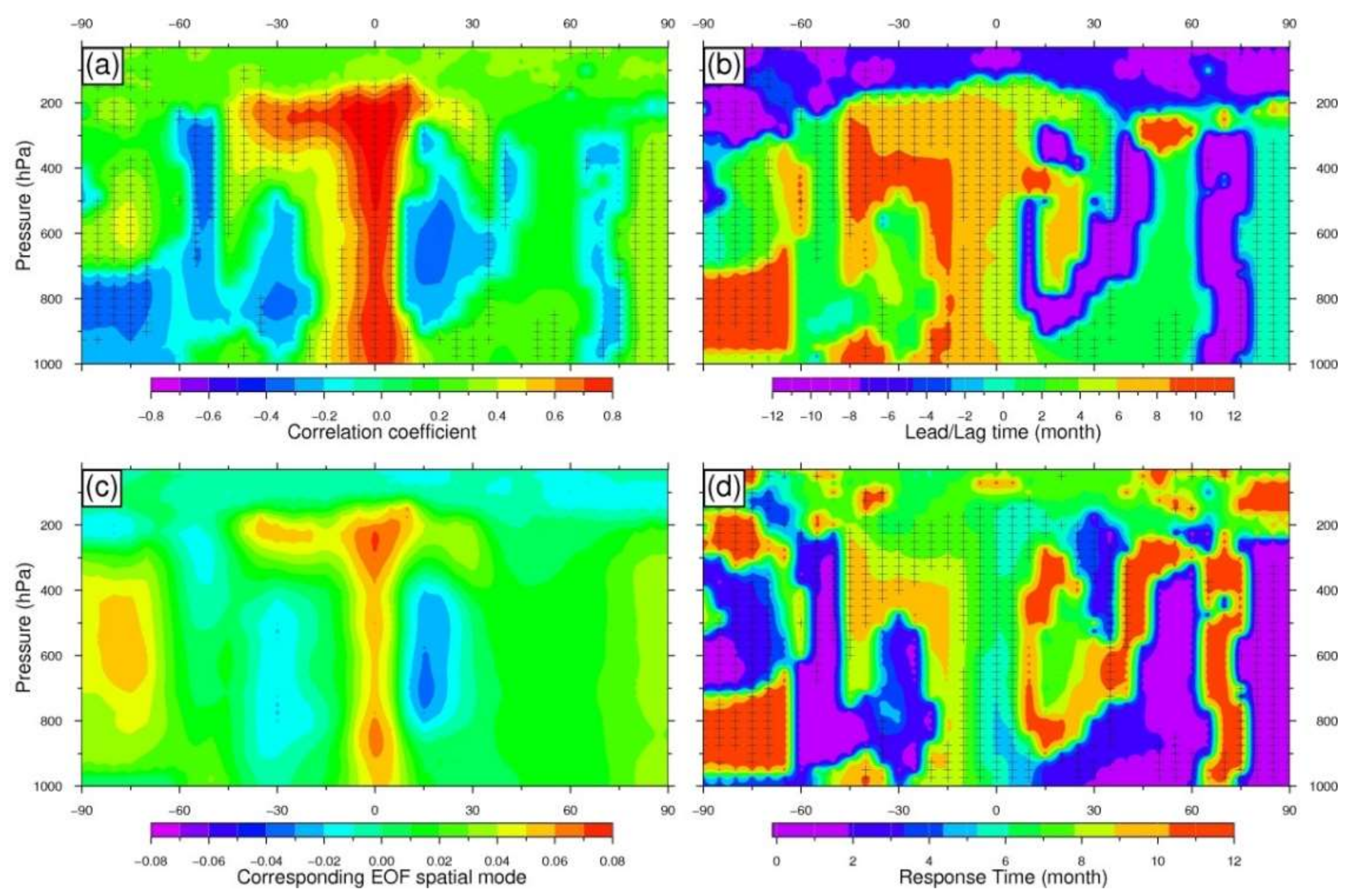
Figure 9 depicts the vertical structure and temporal response to ENSO in the TLS. The correlation coefficient between ENSORS (i.e., extracted from the zonal-mean specific humidity monthly anomalies at different altitudes) and ONI is 0.829 after a delay of four months compared with ONI. The zonal-mean correlation coefficient cross-sections (Figure 9a) present strong positive correlations over the tropical areas in the troposphere with a lag time of 4–8 months (Figure 9b). In the upper troposphere (400–200 hpa), the areas showing strong positive correlations with ENSO extend from the tropics to the latitudes of 45°S–30°N. At the same time, negative correlations are found in the center of and , in the middle and lower troposphere (not significant correlations). Although these areas with negative correlations are not statistically significant, the corresponding EOF spatial mode presented a similar phenomenon (Figure 9c). Negative correlations were also evident over 45°S–60°S in the middle troposphere and over 70°N–75°N in the lower troposphere. Over the high latitudes (70°S–90°S and 75°N–90°N), positive correlations were found in the middle troposphere, and the correlations penetrated downward to the lower troposphere over the Northern high latitudes. Over the Southern high latitudes, negative correlation coefficients were found in the lower troposphere. A similar pattern was observed in the corresponding EOF spatial mode (Figure 9c), specifically over the G30 and high-latitude areas. Figure 9b shows the corresponding temporal responses to ENSO, which were derived from the zonal-mean specific humidity monthly anomalies. Over the tropics, the temporal responses to ENSO present a pattern showing that the larger correlation coefficient between the zonal-mean specific humidity monthly anomaly and ONI is accompanied by a shorter lag time to ONI. These findings are similar to the results from the temporal responses of ENSO at an altitude of 245 hpa across the globe (Figure 8b,d). The corresponding lag time responses of ONI were approximately 0–2 months over the Southern high latitudes (70°S–90°S) in the middle troposphere, Northern high latitudes (75°N–90°N) below 200 hpa in the troposphere, and over 45°S–60°S and 45°N–60°N in the troposphere. Furthermore, the vertical responses to ENSO were very slow (>12 months) in the lower troposphere over the high latitude of the Southern hemisphere, across the center of , and 60°N–75°N in the troposphere (Figure 9d).
4. Conclusions
The ENSORS of specific humidity profiles in the TLS observed by COSMIC were extracted successively by applying an optimal low-pass filter and EOF analysis in the current study. Different altitudes and different regions during the period of June 2006–June 2014 were considered. Given that monthly mean anomalies are affected by several factors besides ENSO, the optimal low-pass filtering method was proposed to eliminate the QBO and other unknown (unmodelled) factors for the different altitudes in the TLS. Then, EOF was conducted to extract the ENSORS. Finally, the spatial and temporal responses to ENSO in the TLS were investigated by the proposed method.
Our findings can be summarized as follows:
(1) The absolute values of the correlation coefficients between ENSORS and ONI based on Scheme 2 (optimal low-pass filtering + EOF) were significantly higher than those of Scheme 1 over the statistical areas in the TLS, especially in the lower stratosphere and lower troposphere. The proposed method used to extract the ENSORS in the TLS was more stable and effective than only using the EOF analysis (Scheme 1). The proposed method can effectively eliminate the influence of QBO in the lower stratosphere and other unknown (unmodelled) factors in the TLS.
(2) The ENSORS can be extracted stably in the middle troposphere and upper troposphere (~560–150 hpa) over different areas containing the N3.4 area (−5°S to 5°N, 120°W to 170°W). The strongest responses were observed in the upper troposphere (250–200 hpa) with a lag time of 3–6 months (2 seasons). The maximum absolute value of the correlation coefficient between the extracted ENSORS and ONI can reach more than 0.94 over the G25–G65 areas. The ENSORS extracted over all the G25–G65 areas presented a similar stable pattern over altitudes of 940–150 hpa. The temporal response to ENSO in the troposphere can delay ONI by 0–6 months (≤). The most suitable areas and altitudes for extracting ENSORS are found over the G25–G65 areas in the upper troposphere (250–200 hpa) with a lag time of 3 months relative to ONI. The good agreement with ONI indicates that the ENSORS extracted by the proposed strategy are useful for monitoring ENSO events.
(3) In the tropical troposphere, ENSORS are the main source of inter-annual variation. The first EOF mode of the N3.4 area corresponds to 83.59% of the total specific humidity anomaly variance at an altitude of 250 hpa. With the expansion of the region, the corresponding EOF modes that can explain the variance decrease gradually at the strongest response altitudes over different areas. Across the globe, the second EOF mode that is correlated with the ONI can explain 10.03% of the total specific humidity anomaly variance at the strongest response altitude (altitude = 245 hpa). Patterns for the temporal and spatial responses to ENSO in the upper troposphere were established in the current study: the larger the correlation coefficient is, the shorter the lag time will be.
(4) In the lower stratosphere, the ENSORS were proven not to be the most prominent source of inter-annual variation. The maximum absolute values of correlation coefficients between the ENSORS and ONI in the lower stratosphere (>0.7) were smaller than those in the troposphere (>0.8) at different altitudes. The extracted ENSORS thus present an unstable pattern at different altitudes.
(5) A clear vertical structure of ENSO in the troposphere was constructed with the ENSORS extracted from the zonal-mean specific humidity monthly anomalies at different altitudes. Strong positive effects were identified over the tropics in the lower and middle troposphere, and they extended from the tropics to the areas of 45°S–30°N in the upper troposphere with a lag time of 4–8 months relative to ONI. At the same time, negative correlations were found at the center of and in the middle and lower troposphere (although these were not statistically significant). Negative correlations were also evident over 45°S–60°S in the middle troposphere and over 70°N–75°N in the lower troposphere.
Above all, the ENSORS can be extracted most effectively and stably over the G25–G65 areas in the upper troposphere (250–200 hpa) at a lag time of 3 months with the proposed method of optimal low-pass filtering and EOF analysis. The spatial and temporal responses to ENSO over different areas have been depicted in detail. With the FORMOSAT-7/COSMIC-2 launched in 2017, which will provide a longer GNSS RO record, the time series of ENSORS will continue to be a good index for monitoring and diagnosing the ENSO events.
Acknowledgments
We thank Kevin Fleming of GFZ Potsdam and another anonymous reviewer for their constructive comments and suggestions on the present work. This work is co-supported by the National Natural Science Foundation of China (Grants No. 41774032, No. 41774033, and No. 41704011), the National Basic Research Program of China (973 Program) (Grant No. 2013CB733302), the Key Laboratory of Geospace Environment and Geodesy, Wuhan University, Ministry of Education (Grant No. 15-02-03), the China Postdoctoral Science Foundation funded project (Grant No. 2017M622451) and the Science and Technology Project of Jiangxi Provincial Education Department (Grant No. GJJ150592). The authors would like to thank all the team members of the COSMIC Data Analysis and Archive Center for providing the datasets. The numerical calculations of this work have been down on the supercomputing system in the Supercomputing Center of Wuhan University. This work made use of GMT software [49].
Author Contributions
All authors significantly contributed to the manuscript and discussed the results. Zhiping Chen and Jia Luo initiated the idea. Zhiping Chen performed all data processing and analyses, and contributed to the manuscript. Jiancheng Li, Jia Luo and Xinyun Cao provided critical comments and contributed to the final revision of the paper.
Conflicts of Interest
The authors declare no conflict of interest.
References
- Hanley, D.E.; Bourassa, M.A.; O’Brien, J.J.; Smith, S.R.; Spade, E.R. A quantitative evaluation of ENSO indices. J. Clim. 2003, 16, 1249–1258. [Google Scholar] [CrossRef]
- Lau, K.-M.; Ho, C.-H.; Kang, I.-S. Anomalous Atmospheric Hydrologic Processes Associated with ENSO: Mechanisms of Hydrologic Cycle-Radiation Interaction. J. Clim. 1998, 11, 800–815. [Google Scholar] [CrossRef]
- McPhaden, M.J.; Zebiak, S.E.; Glantz, M.H. ENSO as an Integrating Concept in Earth Science. Science 2006, 314, 1740–1745. [Google Scholar] [CrossRef] [PubMed]
- Ropelewski, C.F.; Halpert, M.S. Precipitation patterns associated with the high index phase of the Southern Oscillation. J. Clim. 1989, 2, 268–284. [Google Scholar] [CrossRef]
- Ropelewski, C.F.; Halpert, M.S. Global and regional scale precipitation patterns associated with the El Niño/Southern Oscillation. Mon. Weather Rev. 1987, 115, 1606–1626. [Google Scholar] [CrossRef]
- Ropelewski, C.F.; Halpert, M.S. Quantifying southern oscillation-precipitation relationships. J. Clim. 1996, 9, 1043–1059. [Google Scholar] [CrossRef]
- Glantz, M.H.; Katz, R.W.; Nicholls, N. Teleconnections Linking Worldwide Climate Anomalies; Cambridge University Press: Cambridge, UK, 1991. [Google Scholar]
- Rasmusson, E.M.; Wallace, J.M. Meteorological Aspects of the El Niño/Southern Oscillation. Science 1983, 222, 1195–1202. [Google Scholar] [CrossRef] [PubMed]
- Cane, M.A. Oceanographic events during El Niño. Science 1983, 222, 1189–1195. [Google Scholar] [CrossRef] [PubMed]
- Neelin, J.D.; Latif, M. El Niño Dynamics. Phys. Today 1998, 51, 32. [Google Scholar] [CrossRef] [Green Version]
- Tasambay-Salazar, M.; OrtizBeviá, M.J.; Alvarez-García, F.J.; RuizdeElvira, A.M. An estimation of ENSO predictability from its seasonal teleconnections. Theor. Appl. Climatol. 2015, 122, 383–399. [Google Scholar] [CrossRef]
- Steiner, A.K.; Lackner, B.C.; Ladstädter, F.; Scherllin-Pirscher, B.; Foelsche, U.; Kirchengast, G. GPS radio occultation for climate monitoring and change detection. Radio Sci. 2011, 46, RS0D24. [Google Scholar] [CrossRef]
- Scherllin-Pirscher, B.; Deser, C.; Ho, S.P.; Chou, C.; Randel, W.; Kuo, Y.H. The vertical and spatial structure of ENSO in the upper troposphere and lower stratosphere from GPS radio occultation measurements. Geophys. Res. Lett. 2012, 39, L20801. [Google Scholar] [CrossRef]
- Angell, J. Comparison of variations in atmospheric quantities with sea surface temperature variations in the equatorial eastern Pacific. Mon. Weather Rev. 1981, 109, 230–243. [Google Scholar] [CrossRef]
- Angell, J.K. Tropospheric temperature variations adjusted for El Niño, 1958–1998. J. Geophys. Res. Atmos. 2000, 105, 11841–11849. [Google Scholar] [CrossRef]
- Yulaeva, E.; Wallace, J.M. The Signature of ENSO in Global Temperature and Precipitation Fields Derived from the Microwave Sounding Unit. J. Clim. 1994, 7, 1719–1736. [Google Scholar] [CrossRef]
- Lackner, B.C.; Steiner, A.K.; Hegerl, G.C.; Kirchengast, G. Atmospheric climate change detection by radio occultation data using a fingerprinting method. J. Clim. 2011, 24, 5275–5291. [Google Scholar] [CrossRef]
- Fernández, N.C.; García, R.R.; Herrera, R.G.; Puyol, D.G.; Presa, L.G.; Martín, E.H.; Rodríguez, P.R. Analysis of the ENSO signal in tropospheric and stratospheric temperatures observed by MSU,1979–2000. J. Clim. 2004, 17, 3934–3946. [Google Scholar] [CrossRef]
- Su, H.; Neelin, J.D.; Meyerson, J.E. Mechanisms for lagged atmospheric response to ENSO SST forcing. J. Clim. 2005, 18, 4195–4215. [Google Scholar] [CrossRef]
- Christy, J.R.; Drouilhet, S.J., Jr. Variability in daily, zonal mean lower-stratospheric temperatures. J. Clim. 1994, 7, 106–120. [Google Scholar] [CrossRef]
- Free, M.; Seidel, D.J. Observed El Niño–Southern Oscillation temperature signal in the stratosphere. J. Geophys. Res. 2009, 114, D23108. [Google Scholar] [CrossRef]
- García-Herrera, R.; Calvo, N.; Garcia, R.R.; Giorgetta, M.A. Propagation of ENSO temperature signals into the middle atmosphere: A comparison of two general circulation models and ERA-40 reanalysis data. J. Geophys. Res. 2006, 111, D06101. [Google Scholar] [CrossRef]
- Teng, W.-H.; Huang, C.-Y.; Ho, S.-P.; Kuo, Y.-H.; Zhou, X.-J. Characteristics of global precipitable water in ENSO events revealed by COSMIC measurements. J. Geophys. Res. Atmos. 2013, 118, 8411–8425. [Google Scholar] [CrossRef]
- Sun, Y.-Y.; Liu, J.-Y.; Tsai, H.-F.; Lin, C.-H.; Kuo, Y.-H. The Equatorial El Niño-Southern Oscillation Signatures Observed by FORMOSAT-3/COSMIC from July 2006 to January 2012. Terr. Atmos. Ocean. Sci. 2014, 25, 545–558. [Google Scholar] [CrossRef]
- Rasmusson, E.M.; Carpenter, T.H. Variations in Tropical Sea Surface Temperature and Surface Wind Fields Associated with the Sourthern Oscillation/El Nino. Mon. Weather Rev. 1982, 110, 354–384. [Google Scholar] [CrossRef]
- Lau, K.M.; Ho, C.H.; Chou, M.D. Water vapor and cloud feedback over the tropical oceans: Can we use ENSO as a surrogate for climate change? Geophys. Res. Lett. 1996, 23, 2971–2974. [Google Scholar] [CrossRef]
- Trenberth, K.E.; Caron, J.M. The Southern Oscillation revisited: Sea level pressures, surface temperatures, and precipitation. J. Clim. 2000, 13, 4358–4365. [Google Scholar] [CrossRef]
- Sokolovskiy, S.V.; Rocken, C.; Lenschow, D.H.; Kuo, Y.-H.; Anthes, R.A.; Schreiner, W.S.; Hunt, D.C. Observing the moist troposphere with radio occultation signals from COSMIC. Geophys. Res. Lett. 2007, 34, L18802. [Google Scholar] [CrossRef]
- Ahrens, C.D. Meteorology Today: An Introduction to Weather, Climate, and the Environment; Cengage Learning: Boston, MA, USA, 2012. [Google Scholar]
- Fukuoka, A. The Central Meteorological Observatory, A study on 10-day forecast (A synthetic report). Geophys. Mag. 1951, 22, 177–208. [Google Scholar]
- Lorenz, E.N. Empirical Orthogonal Functions and Statistical Weather; Massachusetts Institute of Technology: Cambridge, MA, USA, 1956. [Google Scholar]
- Aires, F.; Chédin, A.; Nadal, J.P. Independent component analysis of multivariate time series: Application to the tropical SST variability. J. Geophys. Res. 2000, 105, 17437–17455. [Google Scholar] [CrossRef]
- Burgers, G.; Stephenson, D.B. The “normality” of El Niño. Geophys. Res. Lett. 1999, 26, 1027–1030. [Google Scholar] [CrossRef]
- Rocken, C.; Kuo, Y.-H.; Schreiner, W.S.; Hunt, D.; Sokolovskiy, S.; McCormick, C. COSMIC System Description. Terr. Atmos. Ocean. Sci. 2000, 11, 21–52. [Google Scholar] [CrossRef]
- Kursinski, E.R.; Hajj, G.A.; Schofield, J.T.; Linfield, R.P.; Hardy, K.R. Observing Earth’s atmosphere with radio occultation measurements using the Global Positioning System. J. Geophys. Res. 1997, 102. [Google Scholar] [CrossRef]
- Kursinski, E.R.; Hajj, G.A.; Leroy, S.S.; Herman, B. The GPS Radio Occultation Technique. Terr. Atmos. Ocean. Sci. 2000, 11, 53–114. [Google Scholar] [CrossRef]
- Smith, E.K.; Weintraub, S. The constants in the equation for atmospheric refractive index at radio frequencies. Proc. IRE 1953, 41, 1035–1037. [Google Scholar] [CrossRef]
- Poli, P.; Joiner, J.; Kursinski, E.R. 1DVAR analysis of temperature and humidity using GPS radio occultation refractivity data. J. Geophys. Res. 2002, 107. [Google Scholar] [CrossRef]
- Healy, S.; Eyre, J. Retrieving temperature, water vapour and surface pressure information from refractive-index profiles derived by radio occultation: A simulation study. Q. J. R. Meteorol. Soc. 2000, 126, 1661–1683. [Google Scholar] [CrossRef]
- Peixoto, J.P.; Oort, A.H. The climatology of relative humidity in the atmosphere. J. Clim. 1996, 9, 3443–3463. [Google Scholar] [CrossRef]
- Ho, S.-P.; Zhou, X.-J.; Kuo, Y.-H.; Hunt, D.; Wang, J.-H. Global Evaluation of Radiosonde Water Vapor Systematic Biases using GPS Radio Occultation from COSMIC and ECMWF Analysis. Remote Sens. 2010, 2, 1320–1330. [Google Scholar] [CrossRef]
- Sun, B.; Reale, A.; Seidel, D.J.; Hunt, D.C. Comparing radiosonde and COSMIC atmospheric profile data to quantify differences among radiosonde types and the effects of imperfect collocation on comparison statistics. J. Geophys. Res. Atmos. 2010, 115, D23104. [Google Scholar] [CrossRef]
- Wang, B.R.; Liu, X.Y.; Wang, J.K. Assessment of COSMIC radio occultation retrieval product using global radiosonde data. Atmos. Meas. Tech. 2013, 6, 1073–1083. [Google Scholar] [CrossRef]
- Trenberth, K.E.; Stepaniak, D.P. Indices of El Niño evolution. J. Clim. 2001, 14, 1697–1701. [Google Scholar] [CrossRef]
- Jin, E.K.; Kinter, J.L., III; Wang, B.; Park, C.-K.; Kang, I.-S.; Kirtman, B.P.; Kug, J.-S.; Kumar, A.; Luo, J.-J.; Schemm, J.; et al. Current status of ENSO prediction skill in coupled ocean–atmosphere models. Clim. Dyn. 2008, 31, 647–664. [Google Scholar] [CrossRef]
- Barnston, A.G.; Tippett, M.K.; L’Heureux, M.L.; Li, S.; DeWitt, D.G. Skill of real-time seasonal ENSO model predictions during 2002-11: Is our capability increasing? Bull. Am. Meteorol. Soc. 2012, 93, 631–651. [Google Scholar] [CrossRef]
- Tasambay-Salazar, M.; OrtizBeviá, M.J.; Alvarez-García, F.J.; de Elvira, A.M.R. The Niño3. 4 region predictability beyond the persistence barrier. Tellus A 2015, 67. [Google Scholar] [CrossRef]
- Oort, A.H.; Yienger, J.J. Observed Interannual Variability in the Hadley Circulation and Its Connection to ENSO. J. Clim. 1996, 9, 2751–2767. [Google Scholar] [CrossRef]
- Wessel, P.; Smith, W.H.F. New, improved version of generic mapping tools released. EOS Trans. AGU 1998, 79, 579. [Google Scholar] [CrossRef]
Figure 1.
El Niño-Southern Oscillation related signals (ENSORS) extraction in the troposphere and lower stratosphere (TLS).
Figure 1.
El Niño-Southern Oscillation related signals (ENSORS) extraction in the troposphere and lower stratosphere (TLS).

Figure 2.
The processing steps for extracting ENSORS at an altitude of 245 hpa: (a) the original specific humidity data; (b) the monthly anomalies from which the mean annual cycle has been subtracted; (c) the monthly anomalies from (b) which have been further eliminated in terms of month-to-month variations with a 1-2-1 binomial filter; (d) the monthly anomalies from (c) which have been further processed by the low-pass filter with the optimal cut-off frequency; (e) the ENSORS extracted from (c) only by the EOF (Scheme 1). The blue curve is the unmoved ENSORS and the red curve is the ENSORS moved forward by 2 months; (f) the ENSORS extracted from (c) by the low-pass filter with the optimal cut-off frequency and EOF (Scheme 2). The blue curve is the unmoved ENSORS, and the red curve is the ENSORS moved forward 5 months.

Figure 3.
Absolute values of the correlation coefficients between ENSORS and ONI over different areas in the TLS. In each subfigure, the red dotted line represents the result when only the EOF was used (Scheme 1) to extract the ENSORS, while the blue solid line represents the result when the proposed method was used (the optimal low-pass filter + EOF, Scheme 2).

Figure 4.
The maximum response to ENSO derived from COSMIC GNSS RO specific humidity at different altitudes in the TLS over different areas which contain the N3.4 area. (a) The corresponding EOF mode when the absolute value of the correlation coefficient reaches the maximum value; (b) the filtering frequency when the absolute value of the correlation coefficient reaches the maximum value; (c) the correlation coefficient between ENSORS extracted from COSMIC GNSS RO specific humidity observations and ONI; (d) the lead/lag time when the absolute value of the correlation coefficient reaches the maximum value. The two dotted black lines in (d) are the lag times of 0 and 6 months, respectively. Positive values in (d) denote lag time, while negative values denote lead times.

Figure 5.
The maximum response to ENSO derived from COSMIC GNSS RO specific humidity at different altitudes in the TLS over the areas, G25–G65. (a) The corresponding EOF mode when the absolute value of the correlation coefficient reaches the maximum value; (b) the filtering frequency when the absolute value of the correlation coefficient reaches the maximum value; (c) the absolute value of the correlation coefficient between ENSORS extracted from COSMIC specific humidity observations and ONI; (d) the lead/lag time when the absolute value of the correlation coefficient reaches the maximum value. The two dotted black lines in (d) are the lag times of 0 and 6 months, respectively. Positive values in (d) denote lag times, while negative values denote the lead times.
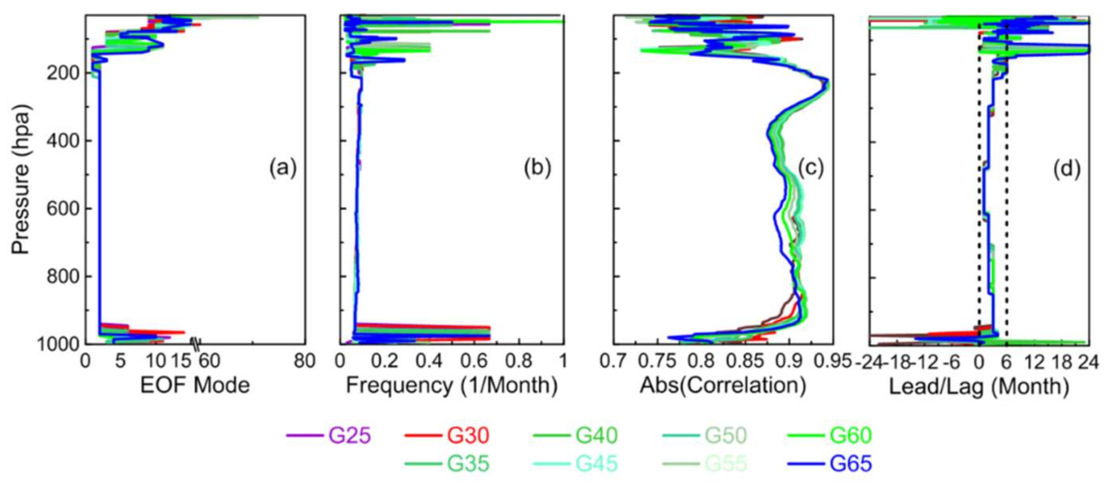
Figure 6.
The maximum response to ENSO derived from COSMIC GNSS RO specific humidity at different altitudes in the TLS over different areas (top: N30, NHM, ARC, and N90; bottom: S30, SHM, ANT, and S90). (a,e) The corresponding EOF modes when the absolute values of the correlation coefficients reach the maximum; (b,f) the corresponding filtering frequencies when the absolute values of the correlation coefficients reach the maximum; (c,g) the absolute values of the correlation coefficients between ENSORS extracted from COSMIC GNSS RO specific humidity observations and ONI; (d,h) the corresponding lag/lead time when the absolute values of the correlation coefficients reach the maximum. The two dotted black lines in (d,h) are the lag times of 0 and 6 months, respectively. Positive values in (d,h) denote lag times, while negative values denote the lead times.

Figure 7.
Normalized specific humidity index and Oceanic Niño index (ONI) time series (red) on the pressure level with the maximum absolute value of correlation between specific humidity and ONI over different areas. ENSORS and ONI are unified as a scale-consistent index by standardized processing.
Figure 7.
Normalized specific humidity index and Oceanic Niño index (ONI) time series (red) on the pressure level with the maximum absolute value of correlation between specific humidity and ONI over different areas. ENSORS and ONI are unified as a scale-consistent index by standardized processing.
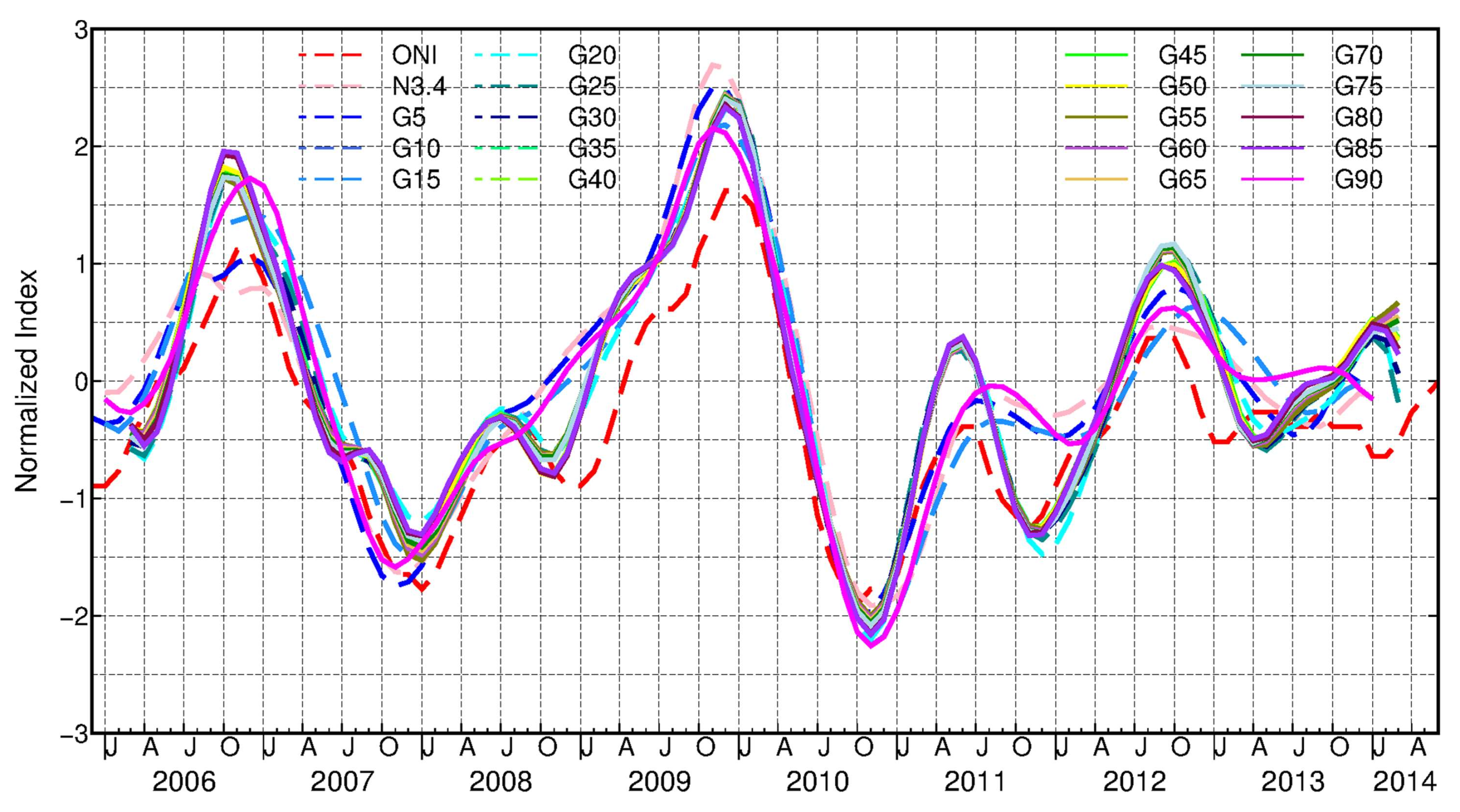
Figure 8.
Spatial and temporal responses to ENSO at an altitude of 245 hpa in the troposphere across the globe. (a) Correlation coefficients between specific humidity anomalies and ONI; (b) the temporal responses at 245 hpa between specific humidity anomalies and ONI (positive values denote lag times and negative values denote lead times); (c) the corresponding EOF spatial mode of the extracted ENSORS when the absolute value of the correlation coefficient reaches the maximum value; (d) the absolute value of corresponding time response when the absolute value of the correlation coefficient reaches the maximum value. Areas with “+” denote significant correlation at the 95% level.
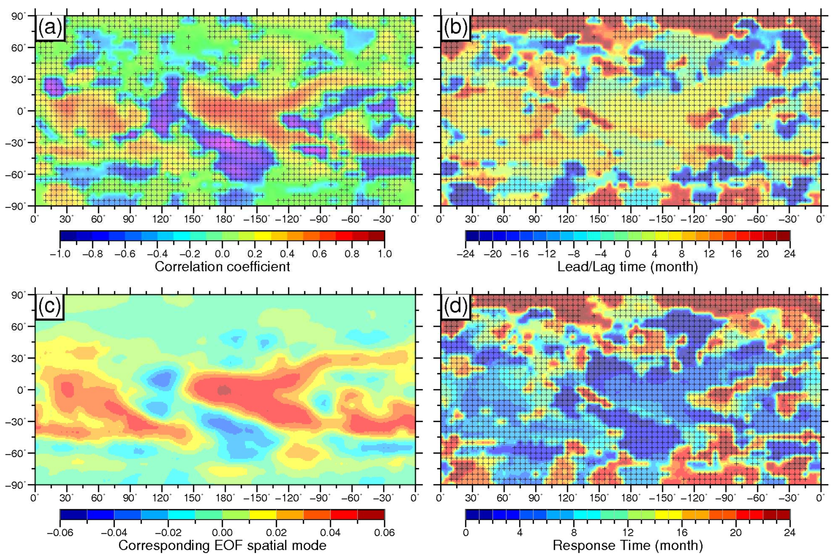
Figure 9.
Zonal mean response to ENSO in the TLS. (a) The meridional cross of the correlation coefficient between monthly anomalies of zonal mean specific humidity and ONI in the TLS; (b) the corresponding time response of ENSO when the absolute value of the correlation coefficient reaches the maximum value; (c) the corresponding EOF spatial mode of the extracted ENSORS when the absolute value of the correlation coefficient reaches the maximum value; (d) the absolute value of the corresponding time response when the absolute value of the correlation coefficient reaches the maximum value. Positive values in (b) denote lag time; negative values in (b) denote the lead time. The maximum correlation was evaluated by Student’s t-test at the 95% confidence level; “+” denotes significant correlation.


Table 1.
Regions defined in this study.
| Abbreviation | Region | Latitude | Longitude |
|---|---|---|---|
| N3.4 | Niño3.4 | −5°S–5°N | 120°W–170°W |
| G5 | Equator | −5°S–5°N | 180°W–180°E |
| G10 | Globe10 | −10°S–10°N | 180°W–180°E |
| G15 | Tropics | −15°S–15°N | 180°W–180°E |
| G20 | Globe20 | −20°S–20°N | 180°W–180°E |
| G25 | Globe25 | −25°S–25°N | 180°W–180°E |
| G30 | Globe30 | −30°S–30°N | 180°W–180°E |
| G35 | Globe35 | −35°S–35°N | 180°W–180°E |
| G40 | Globe40 | −40°S–40°N | 180°W–180°E |
| G45 | Globe45 | −45°S–45°N | 180°W–180°E |
| G50 | Globe50 | −50°S–50°N | 180°W–180°E |
| G55 | Globe55 | −55°S–55°N | 180°W–180°E |
| G60 | Globe60 | −60°S–60°N | 180°W–180°E |
| G65 | Globe65 | −65°S–65°N | 180°W–180°E |
| G70 | Globe70 | −70°S–70°N | 180°W–180°E |
| G75 | Globe75 | −75°S–75°N | 180°W–180°E |
| G80 | Globe80 | −80°S–80°N | 180°W–180°E |
| G85 | Globe85 | −85°S–85°N | 180°W–180°E |
| G90 | Globe90 | −90°S–90°N | 180°W–180°E |
| N30 | Northern30 | 0°N–30°N | 180°W–180°E |
| NHM | Northern Hemisphere Mid-latitudes | 30°N–60°N | 180°W–180°E |
| Arc | Arctic | 60°N–90°N | 180°W–180°E |
| N90 | Northern Hemisphere | 0°N–90°N | 180°W–180°E |
| S30 | Southern30 | 0°S–30°S | 180°W–180°E |
| SHM | Southern Hemisphere Mid-latitudes | 30°S–60°S | 180°W–180°E |
| ANT | Antarctic | 60°S–90°S | 180°W–180°E |
| S90 | Southern Hemisphere | 0°S–90°S | 180°W–180°E |
Table 2.
Extracted ENSORS from different areas containing the N3.4 area in the TLS.
| Areas | Altitudes (hpa) | EOF Mode | Explaining Variance (%) | Filter Range (month) | Maximum Correlation Coefficient | Lag Time (month) |
|---|---|---|---|---|---|---|
| N3.4 | 250 | 1 | 82.59% | 25 | 0.908 | 5 |
| G5 | 210 | 1 | 34.28% | 20.5 | 0.935 | 6 |
| G10 | 225 | 1 | 34.00% | 21 | −0.940 | 6 |
| G15 | 245 | 1 | 31.17% | 21 | 0.937 | 5 |
| G20 | 245 | 2 | 19.32% | 11.5 | 0.937 | 3 |
| G25 | 235 | 2 | 17.10% | 10.5 | 0.938 | 3 |
| G30 | 235 | 2 | 16.30% | 10.5 | 0.943 | 3 |
| G35 | 235 | 2 | 15.47% | 10.5 | 0.945 | 3 |
| G40 | 245 | 2 | 13.93% | 10.5 | 0.944 | 3 |
| G45 | 245 | 2 | 12.65% | 10.5 | 0.943 | 3 |
| G50 | 245 | 2 | 11.57% | 10.5 | 0.942 | 3 |
| G55 | 220 | 2 | 11.44% | 10.5 | 0.942 | 3 |
| G60 | 220 | 2 | 10.70% | 10.5 | 0.943 | 3 |
| G65 | 220 | 2 | 10.00% | 10.5 | 0.943 | 3 |
| G70 | 220 | 2 | 9.36% | 10.5 | 0.942 | 3 |
| G75 | 220 | 2 | 8.84% | 10.5 | 0.940 | 3 |
| G80 | 245 | 2 | 7.71% | 10.5 | 0.938 | 3 |
| G85 | 245 | 2 | 7.31% | 10.5 | 0.937 | 3 |
| G90 | 245 | 2 | 10.03% | 20.5 | -0.936 | 5 |
Table 3.
Extracted ENSORS from different areas excluding the N3.4 area in the TLS.
| Areas | Altitudes (hpa) | EOF Mode | Explaining Variance (%) | Filter Range (month) | Maximum Correlation Coefficient | Lag Time (month) |
|---|---|---|---|---|---|---|
| N30 | 725 | 1 | 21.67% | 26 | 0.924 | 6 |
| NHM | 95 | 15 | 0.12% | 22.5 | 0.877 | 20 |
| ARC | 90 | 8 | 0.72% | 21.5 | 0.898 | 10 |
| N90 | 785 | 4 | 8.38% | 23.5 | 0.936 | 6 |
| S30 | 55 | 10 | 0.40% | 23.5 | 0.921 | 5 |
| SHM | 250 | 2 | 21.25% | 18.5 | 0.918 | 4 |
| ANT | 640 | 8 | 1.91% | 25 | 0.926 | -21 |
| S90 | 240 | 2 | 11.82% | 12 | 0.937 | 3 |
© 2018 by the authors. Licensee MDPI, Basel, Switzerland. This article is an open access article distributed under the terms and conditions of the Creative Commons Attribution (CC BY) license (http://creativecommons.org/licenses/by/4.0/).
Share and Cite
MDPI and ACS Style
Chen, Z.; Li, J.; Luo, J.; Cao, X. A New Strategy for Extracting ENSO Related Signals in the Troposphere and Lower Stratosphere from GNSS RO Specific Humidity Observations. Remote Sens. 2018, 10, 503. https://doi.org/10.3390/rs10040503
AMA Style
Chen Z, Li J, Luo J, Cao X. A New Strategy for Extracting ENSO Related Signals in the Troposphere and Lower Stratosphere from GNSS RO Specific Humidity Observations. Remote Sensing. 2018; 10(4):503. https://doi.org/10.3390/rs10040503
Chicago/Turabian StyleChen, Zhiping, Jiancheng Li, Jia Luo, and Xinyun Cao. 2018. "A New Strategy for Extracting ENSO Related Signals in the Troposphere and Lower Stratosphere from GNSS RO Specific Humidity Observations" Remote Sensing 10, no. 4: 503. https://doi.org/10.3390/rs10040503
Note that from the first issue of 2016, this journal uses article numbers instead of page numbers. See further details here.