Reducing Uncertainties in Applying Remotely Sensed Land Use and Land Cover Maps in Land-Atmosphere Interaction: Identifying Change in Space and Time

Abstract

Land use and land cover (LULC) data are a central component of most land-atmosphere interaction studies, but there are two common and highly problematic scale mismatches between LULC and climate data. First, in the spatial domain, researchers rarely consider the impact of scaling up fine-scale LULC data to match coarse-scale climate datasets. Second, in the temporal domain, climate data typically have sub-daily, daily, monthly, or annual resolution, but LULC datasets often have much coarser (e.g., decadal) resolution. We first explored the effect of three spatial scaling methods on correlations among LULC data and a land surface climatic variable, latent heat flux in China. Scaling by a fractional method preserved significant correlations among LULC data and latent heat flux at all three studied scales (0.5°, 1.0°, and 2.5°), whereas nearest-neighbor and majority-aggregation methods caused these correlations to diminish and even become statistically non-significant at coarser spatial scales (i.e., 2.5°). In the temporal domain, we identified fractional changes in croplands, forests, and grasslands in China using a recently developed and annually resolved time series of LULC maps from 1982 to 2012. Relative to common LULC change (LULCC) analyses conducted over two-time steps or several time periods, this annually resolved, 31-year time series of LULC maps enables robust interpretation of LULCC. Specifically, the annual resolution of these data enabled us to more precisely observe three key and statistically significant LULCC trends and transitions that could have consequential effects on land-atmosphere interaction: (1) decreasing grasslands to increasing croplands in the Northeast China plain and the Yellow river basin, (2) decreasing croplands to increasing forests in the Yangtze river basin, and (3) decreasing grasslands to increasing forests in Southwest China. Our study not only demonstrates the importance of using a fractional spatial rescaling method, but also illustrates the value of annually resolved LULC time series for detecting significant trends and transitions in LULCC, thus potentially facilitating a more robust use of remotely sensed data in land-atmosphere interaction studies.

1. Introduction

Human activities have transformed a large proportion of the planet’s land surface [1] through processes such as the deforestation of tropical forests, as well as intensified agricultural land use and urbanization in China and India. Human-induced land use and land cover change (LULCC) can alter surface roughness, surface wetness, the partitioning of surface energy between sensible and latent heat fluxes, and terrestrial carbon storage [2,3,4,5,6]. These changes are increasingly becoming a focus of concern because of their potential to influence the climate system [7,8] and, as a consequence, the Intergovernmental Panel on Climate Change (IPCC) has emphasized the importance of understanding the climate response to LULCC at local, regional, and global scales [9]. In particular, identifying and quantifying LULCC is crucial for a better understanding of land-atmosphere interaction and thereby climate change and variability [6].

Efforts to map land use and land cover (LULC) and its changing patterns using remotely sensed data have been a focus of much attention over the last three decades [10,11,12,13,14,15]. Remote sensing can potentially provide not only accurate and repeatable global LULC information, but also time series data that can be used to map change [16,17]. However, remotely sensed LULC maps usually have very different spatial resolutions from that of climate data, including atmospheric and oceanic variables. For both physical and observational reasons, climate data generally have much coarser spatial resolution than remotely sensed LULC data. For example, National Center for Environmental Prediction (NCEP)/ National Center for Atmospheric Research (NCAR) reanalysis, European Centre for Medium-Range Weather Forecasts (ECMWF) reanalysis (ERA-40), and Climate Research Unit Time-series (CRU TS) high-resolution gridded datasets have a resolution of 2.5° by 2.5°, 1.125° by 1.125°, and 0.5° by 0.5°, respectively. While anthropogenic forces and other drivers (e.g., natural disturbance from fires or storms, sharp gradients of riparian vegetation) can dramatically alter LULC at fine scales, the atmosphere is often more well mixed, with properties changing more gradually across spatial scales. Simply resampling LULC maps into the same resolution as climate data is problematic, as LULCC is complex, with heterogeneous patterns that may not be evident in simple measures, such as dominant change type, in coarse resolution data.

Problems of spatial scale mismatches are well known to the remote sensing community. For example, Woodcock and Strahler [18] proposed local variance as a framework for examining the effects of scale and spatial resolution in remotely sensed images. They found that traditional spectral classification that produced a single class for each pixel was appropriate where the spatial resolution of the imagery was much finer than the objects in the scene. In contrast, for images where the spatial resolution was not sufficient to resolve the objects, a mixture model, which estimated the proportion of the classes within a pixel, was required [18]. In subsequent work, a more rigorous treatment was developed using variograms [19]. Cao and Lam [20] thoroughly reviewed scale and resolution effects that were relevant to geographic information system (GIS) and remote sensing, and usefully identified four conceptualizations of spatial scale: cartographic scale, geographic (observational) scale, operational scale, and measurement (resolution) scale. In a more recent study, Peng et al. [21] compared several downscaling methods for remotely sensed soil moisture products, including a satellite-based fusion method, a method using geoinformation data, and model-based methods. They concluded that each method has its own advantages and disadvantages, and none of the methods can be applied everywhere across the world without any calibration or improvements [21]. In land-atmosphere interaction studies, the potentially problematic scale effects of the spatial resolution of LULC data and issues of rescaling have been largely overlooked. For example, the Community Earth System Model (CESM) adopted LULC data from Moderate Resolution Imaging Spectroradiometer (MODIS) at 0.05° (approximately 5 km) resolution [22], while the original spatial resolution of MODIS LULC data at that time was 1 km [23]. It is therefore important to identify the effect of different spatial scaling methods for LULC data on land-atmosphere interaction.

Another uncertainty in land-atmosphere interaction studies is due to insufficient LULC time series data to detect long-term LULCC patterns. Cao et al. [24] emphasized that longer time periods of LULC data are needed to quantify land-atmosphere interaction. Currently, there are few continuous annual LULC data, such as MODIS land cover data covering from 2001 onward [25] and European Space Agency (ESA) climate change initiative (CCI) land cover maps covering from 1992 to 2015 [26]. The primary method of extracting LULCC information from remotely sensed data has been through separate classifications of imagery of two different dates, which are overlaid to obtain change information [12]. For example, Rawat and Kumar [27] used 1990 and 2010 Landsat Thematic Mapper (TM) images to classify the land surface of Hawalbagh block, Uttarakhand, India, and thus mapped LULCC over a 20-year period. Similarly, Liu et al. [28] classified cropland based on 1990 and 2000 Landsat TM/ Enhanced Thematic Mapper Plus (ETM+) data to quantify the changing spatial patterns of cropland in China from 1990 to 2000. However, LULCC information from just two-time steps or even several time periods may obscure important overall trends in land cover change, especially in regions where land cover change is dynamic. For example, temporary fluctuations in a landscape where land cover change is common, such as occurs with the logging of short-rotation forests [29], may obscure important long-term trends in land cover change. Change that is non-significant over long time periods could bias analyses that use LULCC as an input or initial forcing for the biophysical and biogeochemical processes of land-atmosphere interaction [30,31,32,33,34,35]. Considering this limitation in recent LULCC detection studies, a spatiotemporal analysis using a long-term time series of LULC maps is an effective option. Such an approach can identify statistically significant spatiotemporal LULCC, as well as provide information regarding the types of LULCC and the dominant transitions among the LULC types.

In this study, we addressed these uncertainties related to the spatial and temporal resolutions of LULC data. Firstly, we used two regions in China (Figure 1): a relatively homogenous region (North China plain), and a more heterogeneous region (Sichuan basin) to explore the effect of LULC spatial resolution on the relationship of LULC data and the land surface climatic variable of latent heat flux. We aggregated the original resolution of the LULC maps from 0.0833° to 0.5°, 1.0°, and 2.5°, which are the commonly used spatial resolutions of climatic variables. At each resolution, we investigated how the correlation of LULC data and latent heat flux is affected by three spatial aggregation methods. We used nearest-neighbor and majority-aggregation methods, which preserve the LULC maps as nominal maps, and a fractional method, which transforms the nominal LULC maps into fractional maps.

Using the optimal scale and scaling method identified in these experiments within the spatial domain, we then explored the temporal changes from 1982 to 2012 for croplands, forests, and grasslands, which are the dominant LULC types in China. Specifically, we used a newly developed 31-year times series of annual LULC maps [36,37] to ask: where are the statistically significant LULCC regions in China based on the long-term time series LULC maps, and what are the dominant transitions among the different types of LULC?

2. Materials and Methods

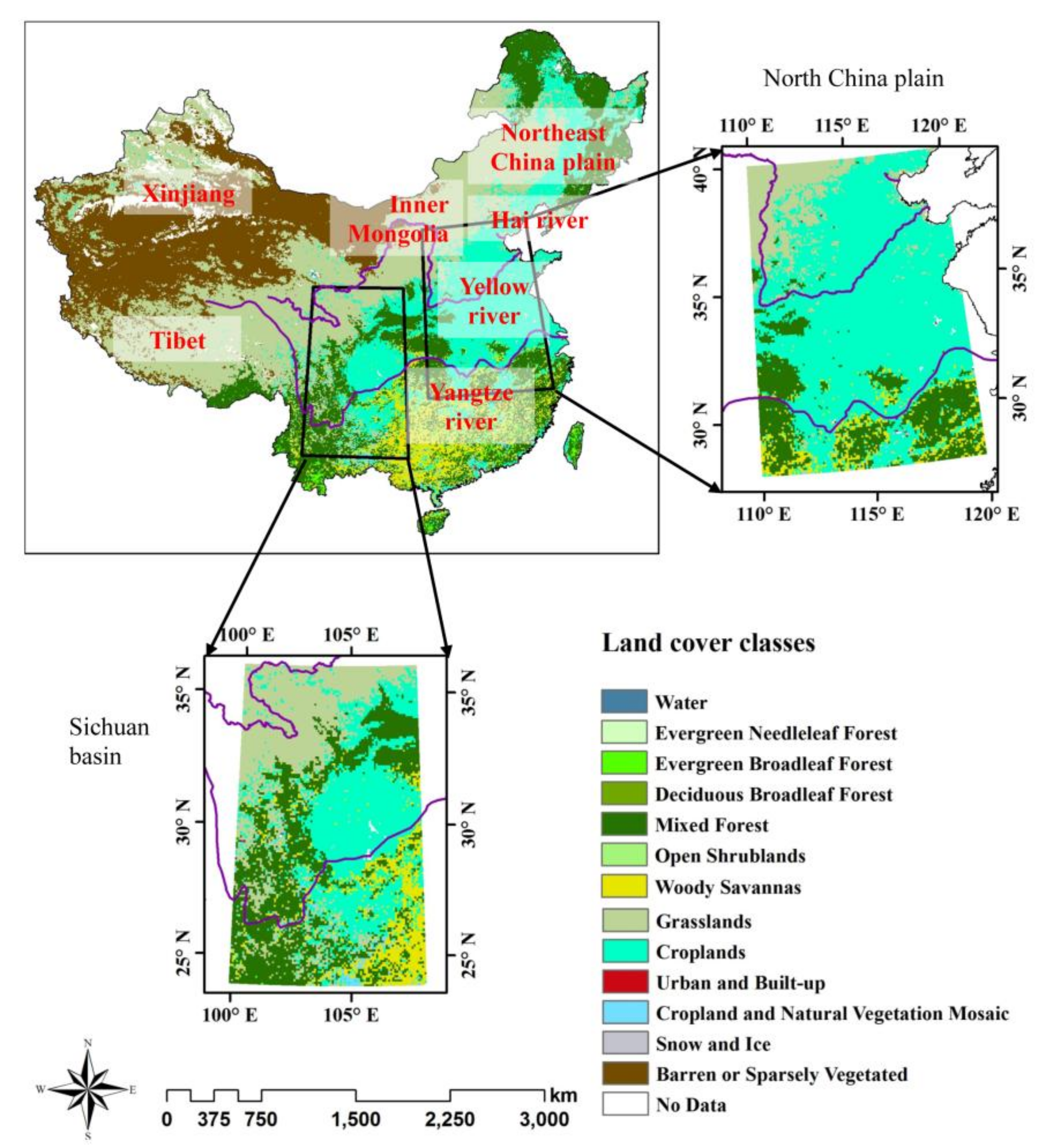
2.1. Materials

The primary dataset used in this study is the continuous annual LULC maps of China, covering the period from 1982 to 2012. Figure 1 shows the LULC map of 2000 as an example. The data were generated by Reference [37] using a random forest classification of 19 phenological metrics derived from the Advanced Very High Resolution Radiometer (AVHRR) Global Inventory Modeling and Mapping Studies (GIMMS) Normalized Difference Vegetation Index third generation (NDVI3g) data. The phenological metrics include the start of growing season, end of growing season, maximum and minimum NDVI values, and so on. The classifier was trained using reference data derived from pixels within the MODIS land cover (MCD12Q1) maps that did not change over the period of 2001 to 2010. The LULCC maps have a 0.0833° (approximately 8 km) spatial resolution and 13 classes, as listed in the legend of Figure 1. The overall accuracy of a simplified eight-class version of the 2012 LULC map was estimated to be 73.8% (refer to He, Lee, and Warner [37] for more information). In order to explore the variation in the relationship between land cover data and climatic variable, we used LULC maps in every six (or five for the last interval) years from the first year of the study period (1982, 1988, 1994, 2000, 2006, and 2011) for spatial rescaling experiments.

As a climatic variable for exploring the effects of rescaling, we chose latent heat flux, because it links the land surface condition to the atmosphere. Latent heat flux data was obtained from the FLUXNET-Multi-Tree Ensemble (MTE). FLUXNET-MTE datasets were estimated using a machine learning approach called model tree ensemble based on FLUXNET measurements, a long-term remotely sensed monthly fraction of absorbed photosynthetically active radiation (fAPAR) dataset, near surface air temperature from Climatic Research Unit (CRU), precipitation data from the Global Precipitation Climatology Center (GPCC), an estimate of the top of the atmosphere shortwave radiation, and information on land cover [38].

The land cover map used in the FLUXNET-MTE dataset did not vary over time [38]. In the MTE model, the land cover data were only used to stratify the data, and did not act as predictor variables for deriving data layers such as the latent heat flux in the regression equations [39]. The global estimates of latent heat flux were similar to other independent estimates [40,41,42] and the R-squared was 0.92 when correlated with catchment water balances [43]. The FLUXNET-MTE dataset has been widely used in hydrology and land-atmosphere interactions studies [43,44,45,46,47]. The spatial resolution of the latent heat flux datasets is 0.5° by 0.5°, over the period of 1982 to 2011. For consistency with the LULC data, latent heat flux during August in 1982, 1988, 1994, 2000, 2006, and 2011 was chosen for the analysis. We chose August because in that month there is a strong relationship between the proportion of croplands and latent heat flux. This is because for croplands August is a time of peak growth and high evapotranspiration, which is directly related to latent heat flux [48].

Although the latent heat flux derived from FLUXNET-MTE can be influenced by land cover types [49,50,51], our objective is to investigate how the relationships between latent heat flux and LULC data derived from different spatial scaling methods (i.e., fractional method, nearest-neighbor method, and majority-aggregation method) change over three different resolutions (i.e., 0.5°, 1.0°, and 2.5°). In doing so, we anticipate identifying the best spatial rescaling method, which can preserve the relationships between latent heat flux and LULC data among different scales.

2.2. Methods

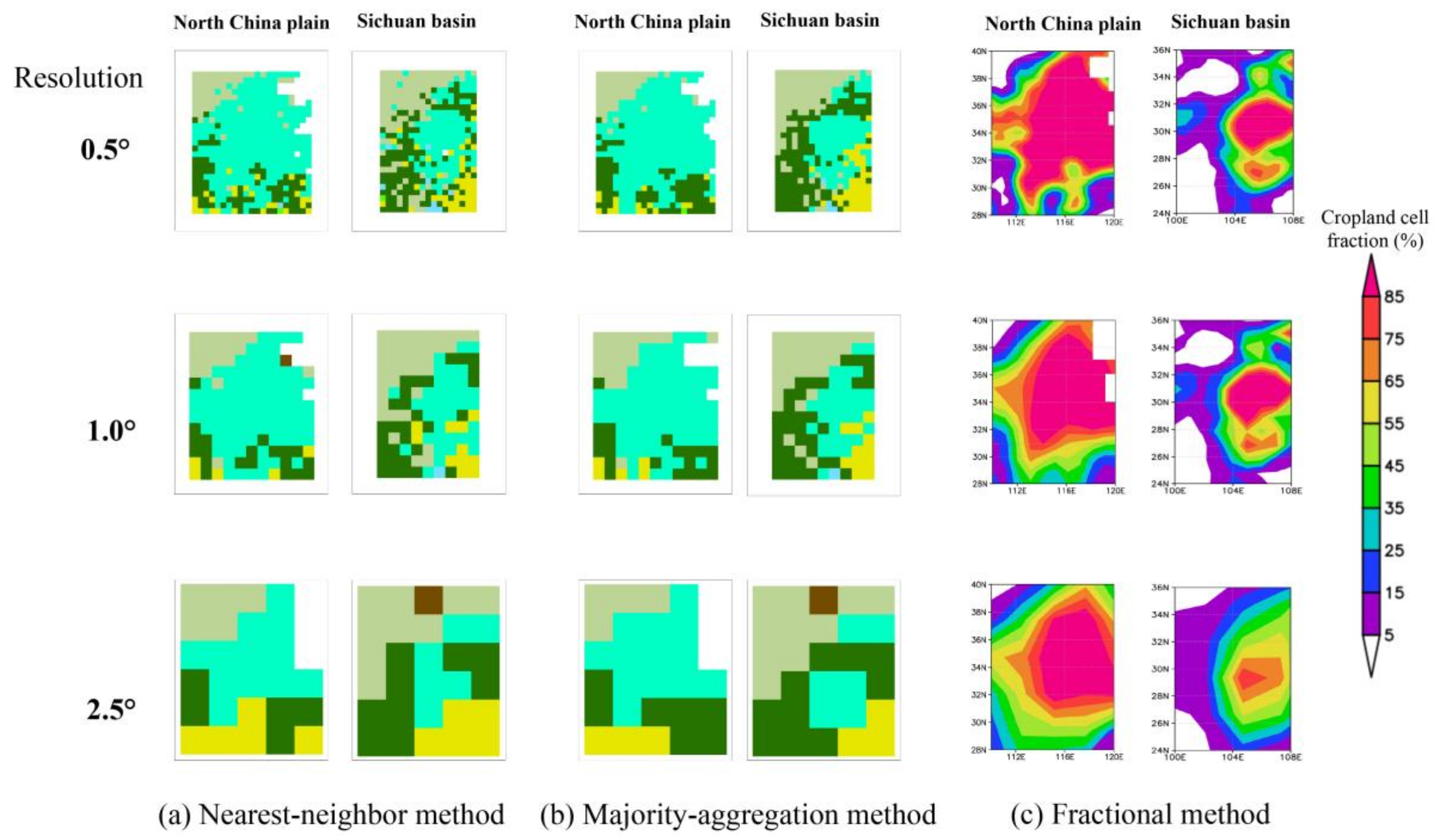
2.2.1. Spatial Scaling Methods

To explore the suitability of different approaches for scaling LULC maps for land-atmosphere interaction studies, we compared three rescaling methods: nearest neighbor, majority aggregation, and a fractional method. The effectiveness of these methods was compared for the aggregation of LULC maps of China with an original 0.0833° spatial resolution, which we rescaled to 0.5°, 1.0°, and 2.5° spatial resolutions.

Nearest-neighbor and majority-aggregation methods, which are commonly used for categorical data such as LULC maps, preserve the nominal nature of LULC maps. In the nearest-neighbor method, the value of an output pixel is determined by the pixel nearest to it in the input data [52]. Majority-aggregation assigns the most frequently occurring value in the input data to the new pixel [37]. The fractional method is a proportional estimate of land cover for each class at the coarser resolution. Specifically, the spatial resolution of the LULC map is aggregated from 0.0833° to 0.5°, 1.0°, and 2.5° by calculating the proportion of the new coarse-scale pixel respectively covered by each class within a 6 × 6, 12 × 12, and 30 × 30 pixel region in the fine-scale data.

We chose bilinear interpolation to resample the latent heat flux data from the original 0.5° to 1.0° and 2.5° spatial resolutions, because it is the method commonly used in the climate community to regrid interval data. In bilinear interpolation, the output pixel value is estimated through the linear interpolation of the four pixel values in two orthogonal directions within the input data [53].

2.2.2. Exploring the Relationship between LULC Data and Latent Heat Flux at Different Spatial Resolutions

For this section, we focused on croplands, because croplands are the dominant LULC type in the North China plain and the Sichuan basin (Figure 1). For fractional LULC maps, we explored relationships between LULC data and latent heat flux by exploring the correlation between the fraction of croplands and latent heat flux. The correlation coefficient is [54]:

$$r=\frac{\sum XY-\frac{\sum X \sum Y}{\mathrm{N}}}{\sqrt{\left(\sum X^2-\frac{{\left(\sum X\right)}^2}{\mathrm{N}}\right)\left(\sum Y^2-\frac{{\left(\sum Y\right)}^2}{\mathrm{N}}\right)}}$$

(1)

where X is the fraction of croplands at different spatial scales in each pixel, and $Y$ is the corresponding August latent heat flux value for each pixel. The significance of the correlation coefficient was tested by the Student’s t-test.

For nominal LULC maps, the relationship between LULC data and latent heat flux was tested by the Wilcoxon rank sum test. The Wilcoxon rank sum test was used to identify the significance of the difference in the distributions of the latent heat flux values in croplands compared to non-croplands. The Wilcoxon rank sum test is a non-parametric test and is suitable for small samples [55]. We chose the Wilcoxon rank sum test because our sample size was proportionally reduced as the spatial scale coarsened.

2.2.3. Linear Regression Trend Analysis

We tested the usefulness of the fractional rescaling method for evaluating trends in land cover change. We aggregated our 31-year LULC maps using the fractional method, and in doing so, generated fractional maps for croplands, forests, and grasslands, respectively. These 31-year fractional maps were summarized through linear regression trend analysis and spatial pattern correlation analysis to determine the long-term LULCC patterns.

Linear regression analysis is a statistical method for analyzing the relationship between two or more variables by evaluating the degree to which one variable can be predicted or explained by the others [56]. The simple linear regression model is:

Y = a + b X + e

(2)

Parameters a and b are the regression coefficients, which are estimated by a least squares method [57]; e is the regression residual. In this study, we were interested in b, the slope of the regression line, which characterized how the $Y$ variables (fraction of croplands, forests, and grasslands, respectively) change over time ($X$). The significance of the trends was estimated using a Student’s t-test. A trend analysis was performed to determine the spatiotemporal changes in croplands, forests, and grasslands for each grid cell independently, and regions where LULCC is significant were thereby identified. Statistically non-significant regions were masked out, and consequently only pixels significant at the 5% level were shown in the maps.

2.2.4. Spatial Pattern Correlation Analysis

Within four regions where statistically significant changes were identified, we performed spatial pattern correlation analysis to investigate the transitions among the LULC types (e.g., grasslands transitioning to croplands, or croplands to forests). The correlation coefficient here is the same as Equation (1). However, the $X$ and $Y$ have a different meaning. Here, $X$ and $Y$ are the trend values (b in the Equation (2)) of croplands, forests, and grasslands at each grid cell, respectively. The significance of correlation coefficient was quantified using an adjusted Student’s t-test, accounting for spatial autocorrelation through a correction of the degrees of freedom of the samples [58].

3. Results and Discussion

3.1. Categorical and Factional LULC Maps at Different Spatial Resolutions in the North China Plain and the Sichuan Basin

The North China plain is a relatively homogenous region, with croplands being dominant. In contrast, the Sichuan basin is a relatively heterogeneous region, with croplands, mixed forests, and grasslands being prevalent (Figure 1). The overall pattern of croplands in the North China plain and the Sichuan basin is evident in both categorical LULC maps and fractional maps at all three spatial scales (Figure 2). However, due to coarsening of the spatial scale, the heterogeneous patterns of croplands are smoothed, especially at the 2.5° scale. Generally speaking, nearest-neighbor, majority-aggregation, and fractional methods capture the croplands patterns better at the finest scale, 0.5°, with notable smoothing at the scales of 1.0° and 2.5°.

3.2. Relationships of Categorical and Fractional LULC Data with Latent Heat Flux at Different Spatial Resolutions in the North China Plain and the Sichuan Basin

The correlation coefficients for the association of fraction of croplands and latent heat flux in both the North China plain and the Sichuan basin change minimally as the spatial scale coarsened for all six years, and in each case are significant at the 1% level (

Table 1. Spatial correlations of annual fraction of croplands with August latent heat flux in 1982, 1988, 1994, 2000, 2006, and 2011 at 0.5°, 1.0°, and 2.5° spatial resolutions in the North China plain and the Sichuan basin.

Year	Correlation Coefficient, r
	0.5° Spatial Resolution		1.0° Spatial Resolution		2.5° Spatial Resolution
	North China Plain	Sichuan Basin	North China Plain	Sichuan Basin	North China Plain	Sichuan Basin
1982	0.50 *	0.44 *	0.59 *	0.47 *	0.53 *	0.55 *
1988	0.62 *	0.49 *	0.69 *	0.56 *	0.64 *	0.59 *
1994	0.53 *	0.63 *	0.62 *	0.65 *	0.58 *	0.64 *
2000	0.55 *	0.44 *	0.60 *	0.51 *	0.59 *	0.54 *
2006	0.65 *	0.35 *	0.70 *	0.45 *	0.70 *	0.48 *
2011	0.63 *	0.51 *	0.71 *	0.57 *	0.70 *	0.57 *
Mean	0.58	0.48	0.65	0.53	0.62	0.56

*: Significant at the 1% level.

). The difference in mean correlation coefficient of the six years among the three spatial resolutions within each of these two regions is quite small (≤0.08). The significant positive correlations are associated with the increased evapotranspiration during the peak growing time of crops. In general, the correlations in the North China plain are larger than those in the Sichuan basin, which may be due to the existence of more croplands in the North China plain (Figure 1).

For the relationships between categorical LULC data and latent heat flux, the distribution of latent heat flux in croplands and non-croplands is different at the 1% significance level for all six years at both the 0.5° and 1.0° scales in the North China plain and the Sichuan basin for both nearest-neighbor and majority-aggregation methods (

Table 2. Wilcoxon rank sum test p-values for differences in the distribution of latent heat flux values over croplands and non-croplands for two spatial scaling methods in 1982, 1988, 1994, 2000, 2006, and 2011 at 0.5°, 1.0°, and 2.5° spatial resolutions in the North China plain.

Year	p-Value of Wilcoxon Rank Sum Test
	0.5° Spatial Resolution		1.0° Spatial Resolution		2.5° Spatial Resolution
	Nearest Neighbor	Majority Aggregation	Nearest Neighbor	Majority Aggregation	Nearest Neighbor	Majority Aggregation
1982	p < 0.01	p < 0.01	p < 0.01	p < 0.01	p = 0.51	p = 0.22
1988	p < 0.01	p < 0.01	p < 0.01	p < 0.01	p = 0.09	p = 0.09
1994	p < 0.01	p < 0.01	p < 0.01	p < 0.01	p = 0.01	p = 0.03
2000	p < 0.01	p < 0.01	p < 0.01	p < 0.01	p = 0.02	p = 0.07
2006	p < 0.01	p < 0.01	p < 0.01	p < 0.01	p < 0.01	p < 0.01
2011	p < 0.01	p < 0.01	p < 0.01	p < 0.01	p < 0.01	p < 0.01

and

Table 3. Same as in Table 2 but in the Sichuan basin.

Year	p-Value of Wilcoxon Rank Sum Test
	0.5° Spatial Resolution		1.0° Spatial Resolution		2.5° Spatial Resolution
	Nearest Neighbor	Majority Aggregation	Nearest Neighbor	Majority Aggregation	Nearest Neighbor	Majority Aggregation
1982	p < 0.01	p < 0.01	p < 0.01	p < 0.01	p = 0.44	p = 0.41
1988	p < 0.01	p < 0.01	p < 0.01	p < 0.01	p = 0.07	p = 0.12
1994	p < 0.01	p < 0.01	p < 0.01	p < 0.01	p = 0.02	p = 0.06
2000	p < 0.01	p < 0.01	p < 0.01	p < 0.01	p = 0.11	p = 0.09
2006	p < 0.01	p < 0.01	p < 0.01	p < 0.01	p = 0.07	p = 0.08
2011	p < 0.01	p < 0.01	p < 0.01	p < 0.01	p = 0.17	p = 0.03

). At the 2.5° scale, the significance level varies among years in the North China plain. The difference of the distribution is significant in 2006 and 2011 at the 1% level, in 1994 at the 5% level, in 1988 and 2000 at the 10% level, and not significant in 1982 for both nearest-neighbor and majority-aggregation methods (Table 2). In the Sichuan basin, the difference of the distribution is not significant at the 2.5° resolution for all six years, excepting 1994 for the nearest-neighbor method and 2011 for the majority-aggregation method, at the 5% level (Table 3). In addition, the significance level decreases more in the more heterogeneous Sichuan basin than in the relatively homogenous North China plain.

In summary, the fractional method preserves the significant relationship between LULC data and latent heat flux for all six years and all three resolutions in both the North China plain and the Sichuan basin, while the nearest-neighbor and majority-aggregation methods cause these correlations to diminish and even become statistically insignificant at coarser scales in some years. Therefore, we recommend rescaling using fractional maps in land-atmosphere studies. Although the different aggregation methods for LULC data lead to different relationships between LULC data and latent heat flux, the bilinear interpolation of latent heat flux may also influence the relationships. It would be interesting to know if the different relationships are due to only the LULC data aggregation or the aggregation methods for both the LULC data and climate data; this needs to be explored further.

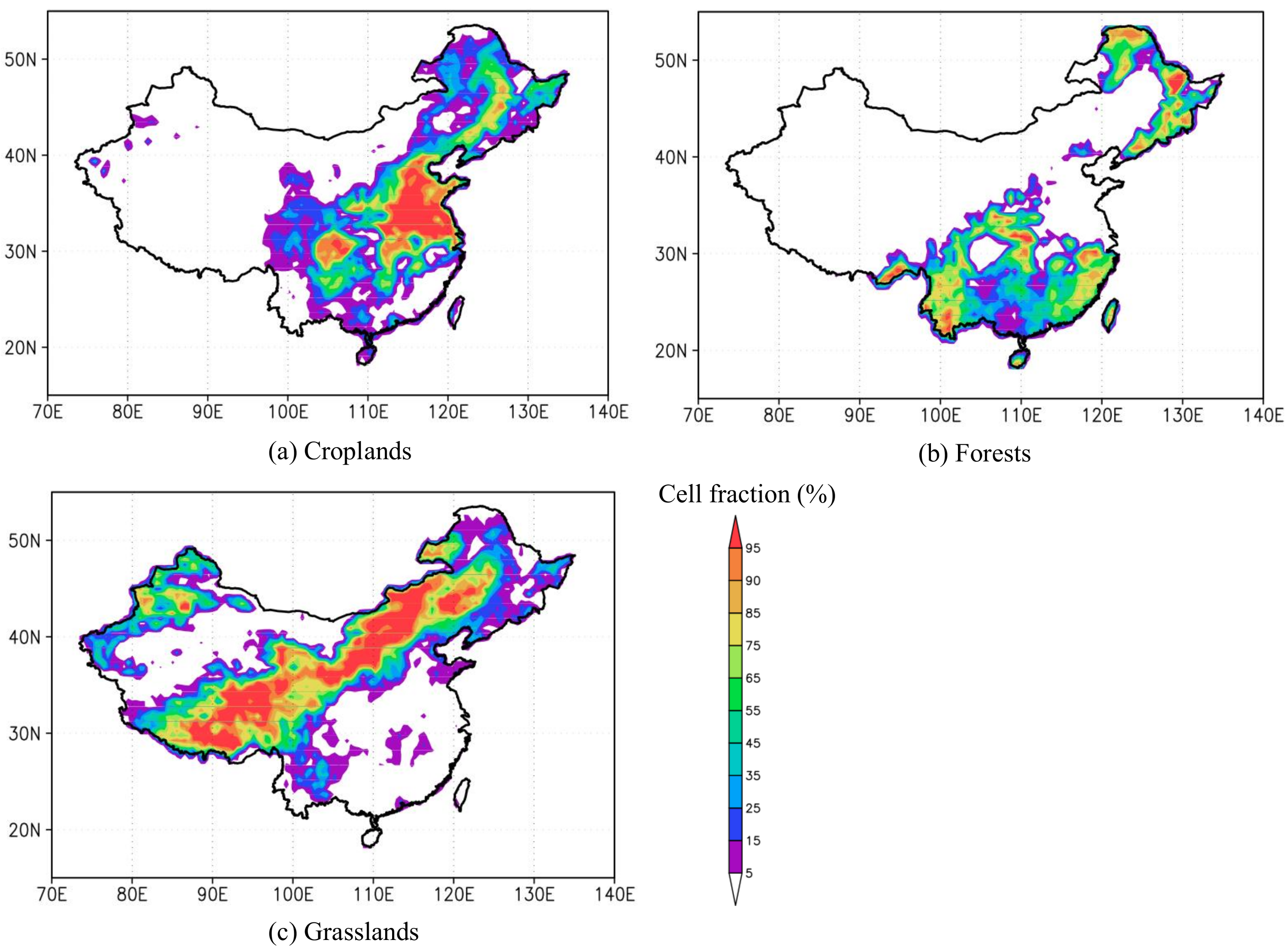
3.3. Fractional Maps of Croplands, Forests, and Grasslands

Based on the aforementioned analyses, the fractional method preserves the significant relationship between LULC data and latent heat flux, and the finer scale (i.e., 0.5° resolution in this study) best captures the spatial patterns. Therefore, we used the fractional method to resample LULC maps to the spatial resolution of 0.5° to identify spatiotemporal changes of croplands, forests, and grasslands from 1982 to 2012 in China. Figure 3 shows the mean fractional maps of croplands, forests, and grasslands averaged over the period of 1982 to 2012. The maps are color coded by the fraction of croplands, forests, and grasslands in each 0.5° grid cell. Figure 3a indicates that croplands dominate in the Northeast China plain, the Hai river basin, the Yellow river basin, the Yangtze river basin, and the Sichuan basin (refer to Figure 1 for the locations of these regions). All of these regions have been recognized as important Chinese agricultural regions since the 11th century [28,59,60,61].

Forests dominate along the borders of the Northeast China, including the mountain ranges of Daxing’anling, Xiaoxing’anling, and Changbaishan, as well as southeast and southwest mountainous regions (Figure 3b). This overall spatial pattern of the distribution of forests in China is consistent with the findings of Yin et al. [62] and Fenning [63]. Grasslands are distributed in a belt, stretching from the Northeast China plain, adjacent to Inner Mongolia, to the Tibetan Plateau. This region covers the major grassland regions of China, including the Hulun Buir and Xilin Gol grasslands in Inner Mongolia and the Naqu grassland in Tibet (Figure 3c). The additional grasslands identified in this study, such as the Narat and Bayinbuluke grasslands in northern Xinjiang province, in far northwestern China, were also identified by Kang et al. [64].

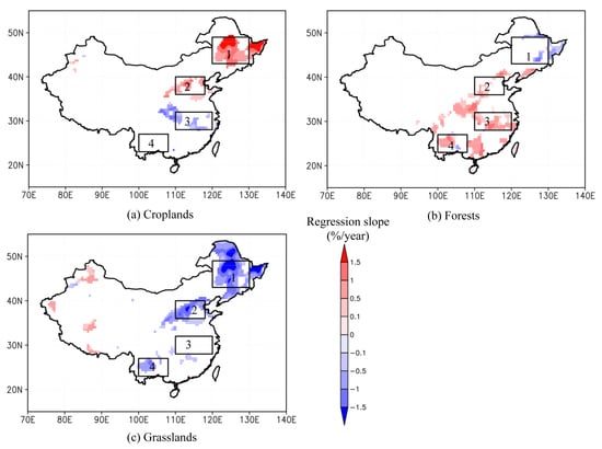
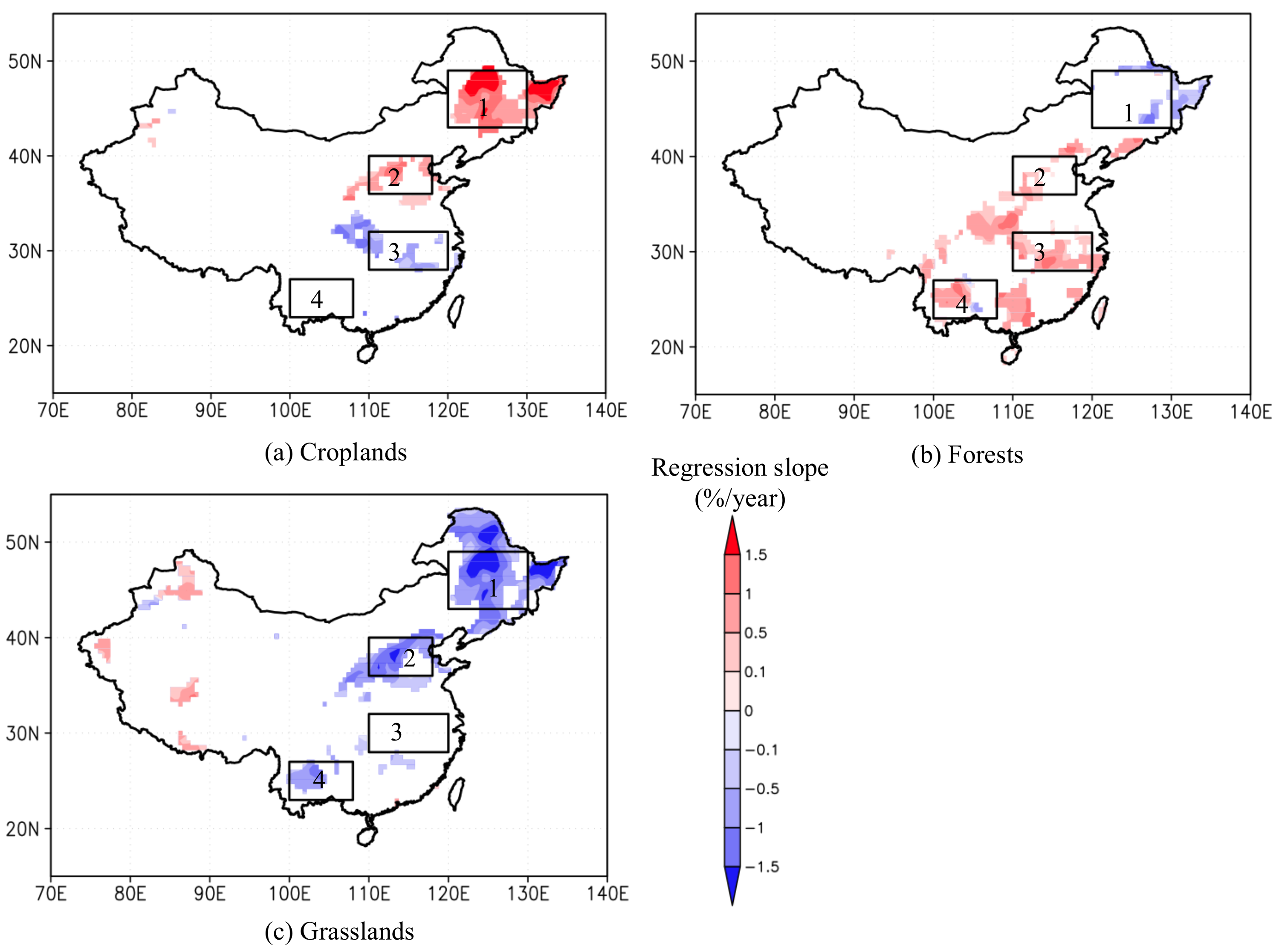
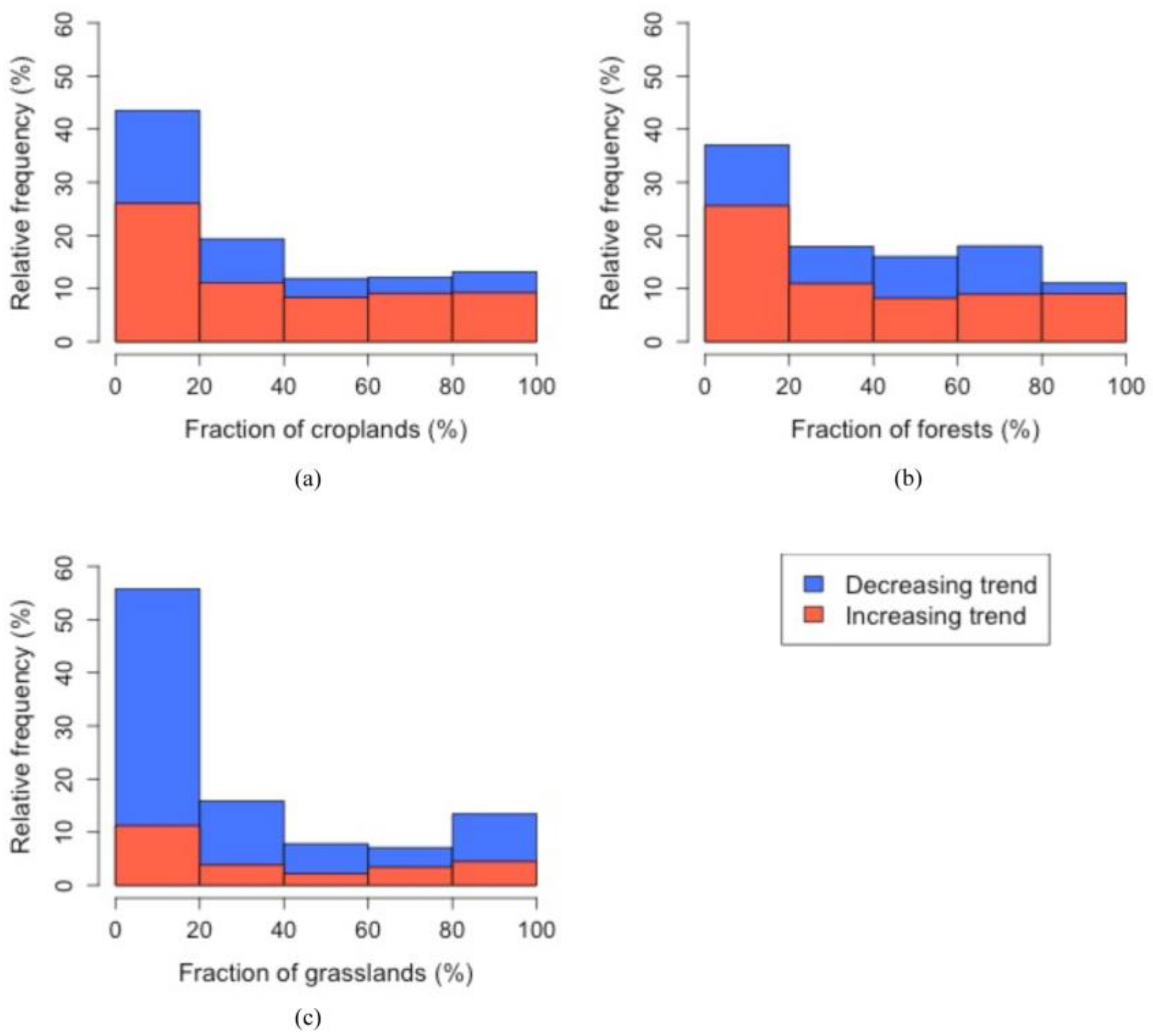
3.4. Spatiotemporal Changes of Croplands, Forests, and Grasslands during the Last Three Decades

The linear regression trend analysis indicates how the fraction of croplands, forests, and grasslands changed from 1982 to 2012 at each grid cell (Figure 4). The color bar represents the slope of the linear regression model over time (i.e., years) for locations where the change is statistically significant at the 5% level. Croplands significantly increased in the Northeast China plain and the Yellow river basin and decreased in the Yangtze river basin (Figure 4a). The highest rate of increase, greater than 1.5%/year, occurred in the Northeast China plain. The increase in croplands in the Northeast China plain may be due to the increase in population, and the associated increase in demand for food [65]. Furthermore, policy regulations such as scrapping the agriculture tax in 2006 and increasing agricultural investment in Northeast China to improve cropland yields in 2008, as well as scientific and technological progress in agriculture including increased access to fertilizer and irrigation and the mechanization of agriculture, may also have all contributed to the increase in croplands [66]. There are also some small isolated areas of significantly increased croplands in the northern part of Xinjiang province, in northwestern China, which may be attributed to the successful promotion of modern agronomic technology [61,67]. The decreased croplands in the Yangtze river basin may be due to increasing forests (Figure 4b), as well as the expansion of industry in that region, which has resulted in arable lands being converted to built-up areas [61]. The overall changing patterns of croplands, especially the increase in North China and the decrease in South China, are consistent with those reported by Liu et al. [62].

In contrast to the trend for croplands, forests significantly decreased along the borders of Northeast China, and increased in the Hai river basin, the Yangtze river basin, and Southwest China (Figure 4b). The increasing trend of forest cover in the Yangtze river basin may be due to the national forest protection project after the catastrophic flood of 1998 [61] and the construction of the forest shelter-belt system [65], which converted other types of LULC, such as croplands, into forest. The increasing trend of forests in southern mountainous areas may be attributed to the “Grain for Green” program and related afforestation activities [65,68]. The reclamation of forests to control sandstorms in the Hai river basin, including the cities of Beijing and Tianjin, is a likely cause of the increasing forests in areas neighboring these two cities.

Grasslands significantly decreased in the Northeast China plain, the Yellow river basin, and Southwest China, and increased in some parts of Western China (Figure 4c). Grassland degradation, which is closely associated with desertification, is a long-term environmental concern in China. The main factors causing grassland degradation are over grazing and cultivation, processes that are common in, for example, Inner Mongolia [69]. However, a revision of the Grassland Law in 2002, which controls all aspects of livestock grazing, may yet result in the recovery of grasslands in Western China (Figure 4c) [69]. The pattern of decreasing grasslands also seems to correspond with an increase in croplands and forests.

Figure 5 summarizes the relative frequency of fraction of croplands, forests, and grasslands for grid cells where the LULCC trend is significant. The histograms show that for all three LULC types, regions with the lowest fractions of LULC (i.e., 0–20%) have the largest number of grid cells with significantly changed LULC, whether the trend is decreasing or increasing, indicating that change tends to occur in cover classes that are a minority proportion of the landscape, rather than the dominant fraction. For croplands and forests, increasing trends are the most common, even where forests and croplands already dominate. For grasslands, decreasing trends dominate, especially for areas where grasslands constitute a low percentage of the land cover even before the additional loss of grassland. In contrast, in areas of moderate percentages of grassland cover (40–80%), increasing and decreasing trends somewhat balance, resulting in only a small net loss of grasslands in such areas.

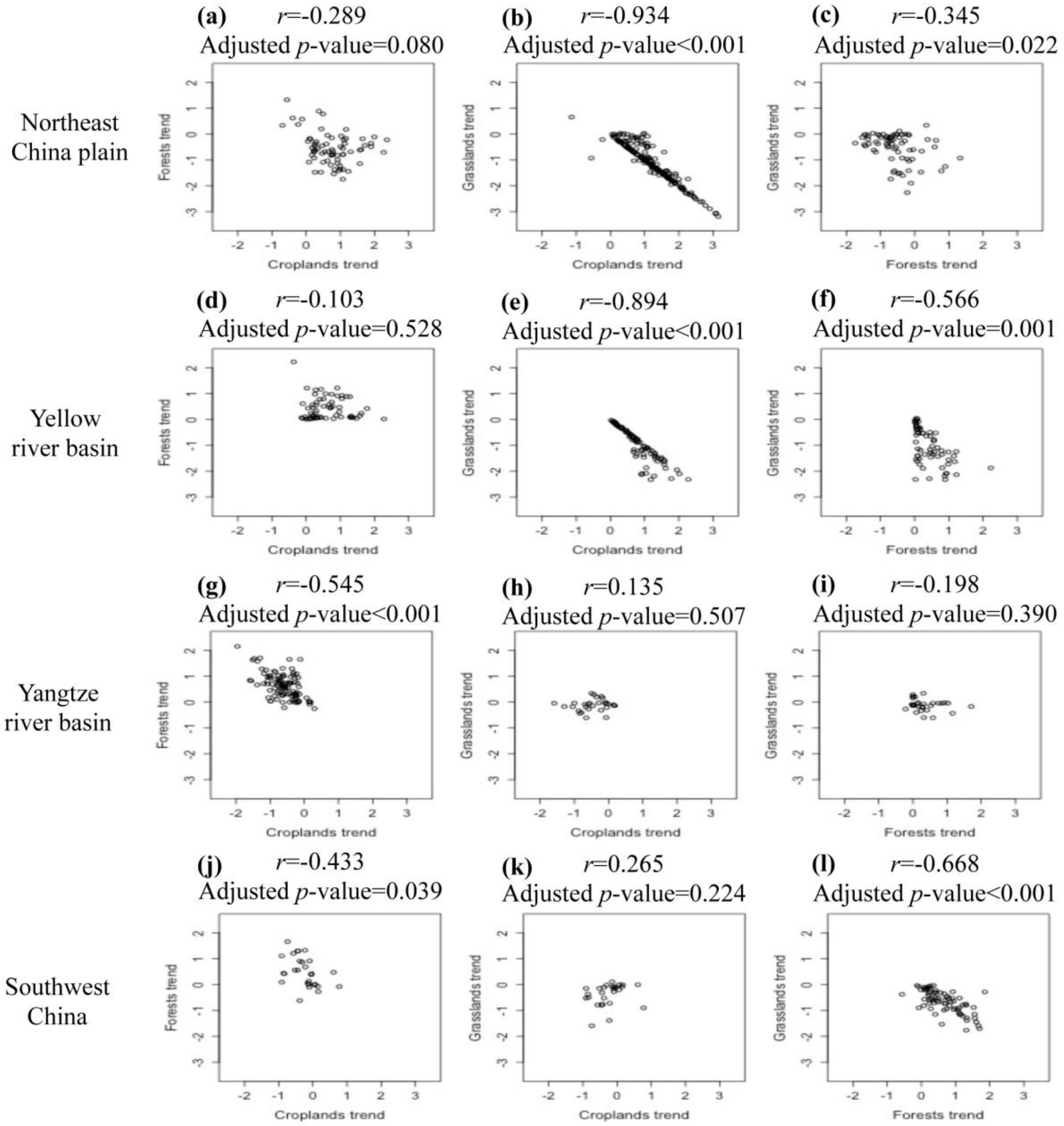
3.5. Transitions between Croplands, Forests, and Grasslands

To examine the underlying relationships among the changes in croplands, forests, and grasslands during the last three decades, we performed spatial pattern correlation analysis, drawing only on grid cells with trends significant at the 5% level. We studied the three LULC types in the selected regions (shown as rectangles in Figure 4): the Northeast China plain (Rectangle 1 in Figure 4), the Yellow river basin (Rectangle 2), the Yangtze river basin (Rectangle 3), and Southwest China (Rectangle 4). Scatterplots and spatial correlation coefficients for the linear regression trends (%/year) of croplands, forests, and grasslands are shown in Figure 6.

The spatial correlation coefficients between croplands, forests, and grasslands in the four regions show very different associations. In the Northeast China plain and the Yellow river basin, grid cells with increasing croplands generally correspond to decreasing grasslands, with a significant negative correlation of r = −0.934 in the Northeast China plain (Figure 6b) and r = −0.894 in the Yellow river basin (Figure 6e). Trends of increased forests are significantly correlated with trends of decreased grasslands in the Yellow river basin (Figure 6f) and the Northeast China plain (Figure 6c). From Figure 6, together with the spatial trends shown in Figure 4, we can draw the general inference that in the Northeast China plain and the Yellow river basin the dominant transition was the replacement of grasslands by croplands. In addition, in the Yellow river basin, grasslands also appear to have been converted to forest cover, though the pattern is less strong than that observed with croplands. In the Yangtze river basin, the only significant association is between decreasing croplands and increasing forests (r = −0.545) (Figure 4 and Figure 6g). In Southwest China, the transition between forests and grasslands has the strongest association (r = −0.668) (Figure 6l), followed by a transition between croplands and forests (r = −0.433) (Figure 4 and Figure 6j).

4. Conclusions

Remotely sensed LULC maps have been widely used in land-atmosphere interaction studies, and this research identified key uncertainties related to scale mismatches in the spatial and temporal domains. Both categorical LULC maps and fractional maps capture the overall pattern of croplands in the relatively homogenous North China plain and the comparatively heterogeneous Sichuan basin at all of the three spatial resolutions studied (0.5°, 1.0°, and 2.5°). The significant positive correlation between the fraction of croplands and latent heat flux in August of 1982, 1988, 1994, 2000, 2006, and 2011 at the three spatial resolutions is quite similar in the two study areas, although the difference in r values between 0.5° and 2.5° is greater in the Sichuan basin than in the North China plain. For the categorical LULC maps, the distribution of latent heat flux values over croplands and non-croplands is significantly different at the 1% level at the 0.5° and 1.0° spatial resolutions for both nearest-neighbor and majority-aggregation methods in North China plain and Sichuan basin for all of the six years. However, at the 2.5° spatial resolution, the significance level varies among years. Nevertheless, both the nearest-neighbor and majority-aggregation methods are particularly problematic in regions with more heterogeneous and fine-grained spatial patterns of LULC. In contrast, for both the relatively homogeneous North China plain and heterogeneous Sichuan basin, the fractional maps preserved the relationships between LULC data and latent heat flux at all of the spatial scales. Therefore, we recommend rescaling using fractional maps in observational land-atmosphere studies. In summary, the fractional scaling method preserves significant correlations among LULC data and latent heat flux at all three studied scales (0.5°, 1.0°, and 2.5°), while nearest-neighbor and majority-aggregation methods cause these correlations to diminish and even become statistically non-significant at coarser scales.

Based on the optimal spatial scaling method, this study explored spatiotemporal changes in croplands, forests, and grasslands from 1982 to 2012 through 31-year LULC maps, which were aggregated to 0.5° using the fractional method. The annual LULC maps enable a time-series analysis of changes in LULC, which is the key attribute compared to the previous LULCC studies of China. Croplands significantly increased in the Northeast China plain and the Yellow river basin, and decreased in the Yangtze river basin. Forests significantly decreased along the border of Northeast China, and increased in the Yangtze river basin and Southwest China. Grasslands significantly decreased in the Northeast China plain, the Yellow river basin, and Southwest China, and increased in some parts of Western China. The analysis of transitions among significant changes in croplands, forests, and grasslands shows that decreasing grasslands in the Northeast China plain and the Yellow river basin are significantly associated with increasing croplands. Similarly, increasing forests in the Yangtze river basin are significantly associated with decreasing croplands. In Southwest China, decreasing grasslands and, to a lesser extent, decreasing croplands, are significantly correlated with the increasing forests.

The time-series analysis of annual LULC maps in China suggests a complex pattern of spatiotemporal changes in croplands, forests, and grasslands from 1982 to 2012. The analysis facilitates the identification of regions where change is extensive and statistically significant, such as North China, where croplands have increased significantly, and South China, where forest have increased significantly. Compared to previous studies, which relied on overlaying LULC maps covering a short-time period [70], the statistically significant patterns of spatiotemporal changes from our study provide a robust approach for capturing LULCC in China.

The identified LULCC patterns in this study have the potential to influence the regional climate in China. The increasing forest in the Yangtze river basin and Southwest China, associated respectively with decreasing of croplands and grasslands, is likely decreasing the region’s albedo, because of the higher albedo of croplands and grasslands compared to forest. A decreased albedo would induce higher net radiation, and consequently promote higher temperatures [7]. On the other hand, the conversions from croplands and grasslands to forests may reduce surface air temperature due to the cooling effects from the higher evapotranspiration of forests [71,72]. The transitions of LULC types within the regions of extensive significant LULCC revealed by this study can potentially alter surface heat and moisture conditions and thereby induce changes in the regional climate system. Previous studies have explored the climatic impacts of LULCC in China. For example, Cao et al. [24] used the weather research and forecasting (WRF) model to investigate how different LULCC types affect regional climate in the agro-pastoral transitional zone of North China. Ma et al. [73] simulated afforestation impacts on the regional climate in Jiangxi province, China using WRF. Fu [32] applied a regional integrated environmental model system (RIEMS) to investigate the effects of human-induced land cover change on the East Asia monsoon. However, most previous studies have not been able to incorporate long-term temporal LULCC patterns due to lack of long-term time series LULC data. Incorporating long-term LULCC pattern, such as that produced in this study, could therefore be useful for future empirical and modeling studies investigating how LULCC affects regional climate.

References

1. Foley, J.A.; DeFries, R.; Asner, G.P.; Barford, C.; Bonan, G.; Carpenter, S.R.; Chapin, F.S.; Coe, M.T.; Daily, G.C.; Gibbs, H.K. Global consequences of land use. Science 2005, 309, 570–574. [Google Scholar] [CrossRef] [PubMed]
2. McPherson, R.A. A review of vegetation—Atmosphere interactions and their influences on mesoscale phenomena. Prog. Phys. Geogr. 2007, 31, 261–285. [Google Scholar] [CrossRef]
3. Pielke, R.A. Land use and climate change. Science 2005, 310, 1625–1626. [Google Scholar] [CrossRef] [PubMed]
4. Foley, J.A.; Costa, M.H.; Delire, C.; Ramankutty, N.; Snyder, P. Green surprise? How terrestrial ecosystems could affect earth’s climate. Front. Ecol. Environ. 2003, 1, 38–44. [Google Scholar]
5. Lee, E.; He, Y.; Zhou, M.; Liang, J. Potential feedback of recent vegetation changes on summer rainfall in the Sahel. Phys. Geogr. 2015, 36, 449–470. [Google Scholar] [CrossRef]
6. Mahmood, R.; Pielke, R.A.; Hubbard, K.G.; Niyogi, D.; Dirmeyer, P.A.; McAlpine, C.; Carleton, A.M.; Hale, R.; Gameda, S.; Beltrán-Przekurat, A. Land cover changes and their biogeophysical effects on climate. Int. J. Climatol. 2014, 34, 929–953. [Google Scholar] [CrossRef]
7. Bonan, G.B.; Pollard, D.; Thompson, S.L. Effects of boreal forest vegetation on global climate. Nature 1992, 359, 716–718. [Google Scholar] [CrossRef]
8. He, Y.; Lee, E. Empirical Relationships of Sea Surface Temperature and Vegetation Activity with Summer Rainfall Variability over the Sahel. Earth Interact. 2016, 20, 1–18. [Google Scholar] [CrossRef]
9. IPCC. Climate Change: Impacts, Adaptation, and Vulnerability; Cambridge University Press: Cambridge, UK; New York, NY, USA, 2014. [Google Scholar]
10. Liu, M.; Tian, H. China’s land cover and land use change from 1700 to 2005: Estimations from high-resolution satellite data and historical archives. Glob. Biogeochem. Cycles 2010, 24, GB3003. [Google Scholar] [CrossRef]
11. Ramankutty, N.; Foley, J.A. Estimating historical changes in global land cover: Croplands from 1700 to 1992. Glob. Biogeochem. Cycles 1999, 13, 997–1027. [Google Scholar] [CrossRef]
12. Liu, J.; Liu, M.; Zhuang, D.; Zhang, Z.; Deng, X. Study on spatial pattern of land-use change in China during 1995–2000. Sci. China Ser. D Earth Sci. 2003, 46, 373–384. [Google Scholar]
13. Liu, J. Macro-Scale Survey and Dynamic Study of Natural Resources and Environment of China by Remote Sensing; China Science and Technology Press: Beijing, China, 1996; pp. 113–124. [Google Scholar]
14. Liu, J.; Zhuang, D.; Ling, Y.; Awaya, Y. Vegetation Integrated Classification and Mapping Using Remote Sensingand GIS Techniques in Northeast China. J. Remote Sens. 1998, 2, 285–291. [Google Scholar]
15. Schneider, A.; Mertes, C. Expansion and growth in Chinese cities, 1978–2010. Environ. Res. Lett. 2014, 9, 024008. [Google Scholar] [CrossRef]
16. Townshend, J.; Justice, C.; Li, W.; Gurney, C.; McManus, J. Global land cover classification by remote sensing: Present capabilities and future possibilities. Remote Sens. Environ. 1991, 35, 243–255. [Google Scholar] [CrossRef]
17. Running, S.W.; Loveland, T.R.; Pierce, L.L. A vegetation classification logic based on remote sensing for use in global biogeochemical models. Ambio 1994, 23, 77–81. [Google Scholar]
18. Woodcock, C.E.; Strahler, A.H. The factor of scale in remote sensing. Remote Sens. Environ. 1987, 21, 311–332. [Google Scholar] [CrossRef]
19. Woodcock, C.E.; Strahler, A.H.; Jupp, D.L. The use of variograms in remote sensing: I. Scene models and simulated images. Remote Sens. Environ. 1988, 25, 323–348. [Google Scholar] [CrossRef]
20. Cao, C.; Lam, N.S.-N. Understanding the scale and resolution effects in remote sensing and GIS. In Scale in Remote Sensing and GIS; Quattrochi, D.A., Goodchild, M.F., Eds.; CRC Press: Boca Raton, FL, USA, 1997; pp. 57–72. [Google Scholar]
21. Peng, J.; Loew, A.; Merlin, O.; Verhoest, N.E. A review of spatial downscaling of satellite remotely sensed soil moisture. Rev. Geophys. 2017, 55, 341–366. [Google Scholar] [CrossRef]
22. Lawrence, P.J.; Chase, T.N. Representing a new MODIS consistent land surface in the Community Land Model (CLM 3.0). J. Geophys. Res. Biogeosci. 2007, 112, G01023. [Google Scholar] [CrossRef]
23. Friedl, M.A.; McIver, D.K.; Hodges, J.C.; Zhang, X.; Muchoney, D.; Strahler, A.H.; Woodcock, C.E.; Gopal, S.; Schneider, A.; Cooper, A. Global land cover mapping from MODIS: Algorithms and early results. Remote Sens. Environ. 2002, 83, 287–302. [Google Scholar] [CrossRef]
24. Cao, Q.; Yu, D.; Georgescu, M.; Han, Z.; Wu, J. Impacts of land use and land cover change on regional climate: A case study in the agro-pastoral transitional zone of China. Environ. Res. Lett. 2015, 10, 124025. [Google Scholar] [CrossRef]
25. Friedl, M.A.; Sulla-Menashe, D.; Tan, B.; Schneider, A.; Ramankutty, N.; Sibley, A.; Huang, X. MODIS Collection 5 global land cover: Algorithm refinements and characterization of new datasets. Remote Sens. Environ. 2010, 114, 168–182. [Google Scholar] [CrossRef]
26. ESA. Land Cover CCI Product User Guide Version 2.0. http://maps.elie.ucl.ac.be/CCI/viewer/download/ESACCI-LC-Ph2-PUGv2_2.0.pdf (accessed on 15 March 2018).
27. Rawat, J.; Kumar, M. Monitoring land use/cover change using remote sensing and GIS techniques: A case study of Hawalbagh block, district Almora, Uttarakhand, India. Egypt. J. Remote Sens. Space Sci. 2015, 18, 77–84. [Google Scholar] [CrossRef]
28. Liu, J.; Liu, M.; Tian, H.; Zhuang, D.; Zhang, Z.; Zhang, W.; Tang, X.; Deng, X. Spatial and temporal patterns of China’s cropland during 1990–2000: An analysis based on Landsat TM data. Remote Sens. Environ. 2005, 98, 442–456. [Google Scholar] [CrossRef]
29. Qiao, H.; Wu, M.; Shakir, M.; Wang, L.; Kang, J.; Niu, Z. Classification of Small-Scale Eucalyptus Plantations Based on NDVI Time Series Obtained from Multiple High-Resolution Datasets. Remote Sens. 2016, 8, 117. [Google Scholar] [CrossRef]
30. Lee, E.; Sacks, W.J.; Chase, T.N.; Foley, J.A. Simulated impacts of irrigation on the atmospheric circulation over Asia. J. Geophys. Res. Atmos. 2011, 116, D08114. [Google Scholar] [CrossRef]
31. Xue, Y. The impact of desertification in the Mongolian and the Inner Mongolian grassland on the regional climate. J. Clim. 1996, 9, 2173–2189. [Google Scholar] [CrossRef]
32. Fu, C. Potential impacts of human-induced land cover change on East Asia monsoon. Glob. Planet. Chang. 2003, 37, 219–229. [Google Scholar] [CrossRef]
33. Jones, P.; Lister, D.; Li, Q. Urbanization effects in large-scale temperature records, with an emphasis on China. J. Geophys. Res. Atmos. 2008, 113, D16122. [Google Scholar] [CrossRef]
34. Han, S.; Yang, Z. Cooling effect of agricultural irrigation over Xinjiang, Northwest China from 1959 to 2006. Environ. Res. Lett. 2013, 8, 024039. [Google Scholar] [CrossRef]
35. Chen, L.; Dirmeyer, P.A. Adapting observationally based metrics of biogeophysical feedbacks from land cover/land use change to climate modeling. Environ. Res. Lett. 2016, 11, 034002. [Google Scholar] [CrossRef]
36. He, Y.; Lee, E.; Warner, T.A. Continuous annual land use and land cover mapping using AVHRR GIMMS NDVI3g and MODIS MCD12Q1 datasets over China from 1982 to 2012. In Proceedings of the IEEE International Geoscience and Remote Sensing Symposium (IGARSS), Beijing, China, 10–15 July 2016; pp. 5470–5472. [Google Scholar]
37. He, Y.; Lee, E.; Warner, T.A. A time series of annual land use and land cover maps of China from 1982 to 2012 generated using AVHRR GIMMS NDVI3g data. Remote Sens. Environ. 2017, 199, 201–217. [Google Scholar] [CrossRef]
38. Jung, M.; Reichstein, M.; Margolis, H.A.; Cescatti, A.; Richardson, A.D.; Arain, M.A.; Arneth, A.; Bernhofer, C.; Bonal, D.; Chen, J. Global patterns of land-atmosphere fluxes of carbon dioxide, latent heat, and sensible heat derived from eddy covariance, satellite, and meteorological observations. J. Geophys. Res. Biogeosci. 2011, 116, G00J07. [Google Scholar] [CrossRef]
39. Jung, M.; Reichstein, M.; Bondeau, A. Towards global empirical upscaling of FLUXNET eddy covariance observations: Validation of a model tree ensemble approach using a biosphere model. Biogeosciences 2009, 6, 2001–2013. [Google Scholar]
40. Oki, T.; Kanae, S. Global hydrological cycles and world water resources. Science 2006, 313, 1068–1072. [Google Scholar] [CrossRef] [PubMed]
41. Trenberth, K.E.; Fasullo, J.T.; Kiehl, J. Earth’s global energy budget. Bull. Am. Meteorol. Soc. 2009, 90, 311–323. [Google Scholar] [CrossRef]
42. Dirmeyer, P.A.; Gao, X.; Zhao, M.; Guo, Z.; Oki, T.; Hanasaki, N. The Second Global Soil Wetness Project (GSWP-2): Multi-model analysis and implications for our perception of the land surface. Bull. Am. Meteorol. Soc. 2006, 87, 1381–1397. [Google Scholar] [CrossRef]
43. Jung, M.; Reichstein, M.; Ciais, P.; Seneviratne, S.I.; Sheffield, J.; Goulden, M.L.; Bonan, G.; Cescatti, A.; Chen, J.; De Jeu, R. Recent decline in the global land evapotranspiration trend due to limited moisture supply. Nature 2010, 467, 951. [Google Scholar] [CrossRef] [PubMed]
44. Bonan, G.B.; Lawrence, P.J.; Oleson, K.W.; Levis, S.; Jung, M.; Reichstein, M.; Lawrence, D.M.; Swenson, S.C. Improving canopy processes in the Community Land Model version 4 (CLM4) using global flux fields empirically inferred from FLUXNET data. J. Geophys. Res. Biogeosci. 2011, 116, G02014. [Google Scholar] [CrossRef]
45. Liu, M.; Tian, H.; Yang, Q.; Yang, J.; Song, X.; Lohrenz, S.E.; Cai, W.J. Long-term trends in evapotranspiration and runoff over the drainage basins of the Gulf of Mexico during 1901–2008. Water Resour. Res. 2013, 49, 1988–2012. [Google Scholar] [CrossRef]
46. Koster, R.D.; Mahanama, S.P. Land surface controls on hydroclimatic means and variability. J. Hydrometeorol. 2012, 13, 1604–1620. [Google Scholar] [CrossRef]
47. Pan, S.; Tian, H.; Dangal, S.R.; Yang, Q.; Yang, J.; Lu, C.; Tao, B.; Ren, W.; Ouyang, Z. Responses of global terrestrial evapotranspiration to climate change and increasing atmospheric CO2 in the 21st century. Earths Future 2015, 3, 15–35. [Google Scholar] [CrossRef]
48. Burba, G.G.; Verma, S.B. Seasonal and interannual variability in evapotranspiration of native tallgrass prairie and cultivated wheat ecosystems. Agric. For. Meteorol. 2005, 135, 190–201. [Google Scholar] [CrossRef]
49. Yang, Z.L.; Dai, Y.; Dickinson, R.; Shuttleworth, W. Sensitivity of ground heat flux to vegetation cover fraction and leaf area index. J. Geophys. Res. Atmos. 1999, 104, 19505–19514. [Google Scholar] [CrossRef]
50. Biraud, S.C.; Riley, W.J.; Fischer, M.L.; Torn, M.S.; Berry, J.A. Spatially Distributed CO2, Sensible, and Latent Heat Fluxes over the Southern Great Plains; Lawrence Berkeley National Laboratory: Berkeley, CA, USA, 2005. [Google Scholar]
51. Williams, I.N.; Torn, M.S. Vegetation controls on surface heat flux partitioning, and land-atmosphere coupling. Geophys. Res. Lett. 2015, 42, 9416–9424. [Google Scholar] [CrossRef]
52. Baboo, S.S.; Devi, M.R. An analysis of different resampling methods in Coimbatore, District. Glob. J. Comput. Sci. Technol. 2010, 10, 61–66. [Google Scholar]
53. Han, P.; Li, Z.; Gong, J. Effects of aggregation methods on image classification. In Geospatial Technology for Earth Observation; Springer: Berlin, Germany, 2010; pp. 271–288. [Google Scholar]
54. Pearson, K. Note on regression and inheritance in the case of two parents. Proc. R. Soc. Lond. 1895, 58, 240–242. [Google Scholar] [CrossRef]
55. Hogg, R.V.; Tanis, E.; Zimmerman, D. Probability and Statistical Inference; Pearson Higher Ed: London, UK, 2014. [Google Scholar]
56. Freund, R.J.; Wilson, W.J.; Sa, P. Regression Analysis; Academic Press: Cambridge, MA, USA, 2006. [Google Scholar]
57. Walpole, R.E.; Myers, R.H.; Myers, S.L.; Ye, K. Probability and Statistics for Engineers and Scientists; Macmillan: New York, NY, USA, 1993. [Google Scholar]
58. Clifford, P.; Richardson, S.; Hémon, D. Assessing the significance of the correlation between two spatial processes. Biometrics 1989, 45, 123–134. [Google Scholar] [CrossRef] [PubMed]
59. Deng, J.; Chuangjun, W.; Zhikang, X. General View of Agriculture Geography of China; Science Press: Beijing, China, 1983; p. 334. [Google Scholar]
60. Korontzi, S.; McCarty, J.; Loboda, T.; Kumar, S.; Justice, C. Global distribution of agricultural fires in croplands from 3 years of Moderate Resolution Imaging Spectroradiometer (MODIS) data. Glob. Biogeochem. Cycles 2006, 20, GB2021. [Google Scholar] [CrossRef]
61. Liu, J.; Zhang, Z.; Xu, X.; Kuang, W.; Zhou, W.; Zhang, S.; Li, R.; Yan, C.; Yu, D.; Wu, S. Spatial patterns and driving forces of land use change in China during the early 21st century. J. Geogr. Sci. 2010, 20, 483–494. [Google Scholar] [CrossRef]
62. Yin, G.; Zhang, Y.; Sun, Y.; Wang, T.; Zeng, Z.; Piao, S. MODIS Based Estimation of Forest Aboveground Biomass in China. PLoS ONE 2015, 10, e0130143. [Google Scholar] [CrossRef] [PubMed]
63. Fenning, T. Challenges and Opportunities for the World’s Forests in the 21st Century; Springer: Dordrecht, The Netherlands, 2014. [Google Scholar]
64. Kang, L.; Han, X.; Zhang, Z.; Sun, O.J. Grassland ecosystems in China: Review of current knowledge and research advancement. Philos. Trans. R. Soc. Lond. B Biol. Sci. 2007, 362, 997–1008. [Google Scholar] [CrossRef] [PubMed]
65. Liu, J.; Kuang, W.; Zhang, Z.; Xu, X.; Qin, Y.; Ning, J.; Zhou, W.; Zhang, S.; Li, R.; Yan, C. Spatiotemporal characteristics, patterns, and causes of land-use changes in China since the late 1980s. J. Geogr. Sci. 2014, 24, 195–210. [Google Scholar] [CrossRef]
66. Man, W.; Wang, Z.; Liu, M.; Lu, C.; Jia, M.; Mao, D.; Ren, C. Spatio-temporal dynamics analysis of cropland in Northeast China during 1990–2013 based on remote sensing. Trans. Chin. Soc. Agric. Eng. 2016, 32, 1–10. [Google Scholar]
67. Yin, X. Analysis on the change of land use by remote sensing technology in Manas county. J. Shihezi Univ. 2008, 26, 402–406. [Google Scholar]
68. Tong, X.; Brandt, M.; Yue, Y.; Horion, S.; Wang, K.; De Keersmaecker, W.; Tian, F.; Schurgers, G.; Xiao, X.; Luo, Y. Increased vegetation growth and carbon stock in China karst via ecological engineering. Nat. Sustain. 2018, 1, 44. [Google Scholar] [CrossRef]
69. Waldron, S.; Brown, C.; Longworth, J. An assessment of China’s approach to grassland degradation and livelihood problems in the pastoral region. In Proceedings of the 5th Annual Conference of the Consortium for Western China Development Studies, Xi’an, China, 22–24 July 2008. [Google Scholar]
70. Fan, F.; Weng, Q.; Wang, Y. Land use and land cover change in Guangzhou, China, from 1998 to 2003, based on Landsat TM/ETM+ imagery. Sensors 2007, 7, 1323–1342. [Google Scholar] [CrossRef]
71. Li, Y.; Zhao, M.; Motesharrei, S.; Mu, Q.; Kalnay, E.; Li, S. Local cooling and warming effects of forests based on satellite observations. Nat. Commun. 2015, 6, 6603. [Google Scholar] [CrossRef] [PubMed]
72. Betts, R.A. Climate science: Afforestation cools more or less. Nat. Geosci. 2011, 4, 504–505. [Google Scholar] [CrossRef]
73. Ma, E.; Liu, A.; Li, X.; Wu, F.; Zhan, J. Impacts of vegetation change on the regional surface climate: A scenario-based analysis of afforestation in Jiangxi Province, China. Adv. Meteorol. 2013, 2013, 148–152. [Google Scholar] [CrossRef]
Figure 1. Land use and land cover map of China from 2000, with the North China plain and Sichuan basin subsets used in the spatial rescaling experiments shown. The geographic locations labeled in red are referred to in Section 3, Results.
Remotesensing 10 00506 g001
Figure 2. Categorical and fractional land use and land cover maps of 2000 in North China plain and Sichuan basin at 0.5°, 1.0°, and 2.5° spatial resolutions, aggregated by (a) the nearest-neighbor method, (b) the majority-aggregation method (please refer to Figure 1 for legend), and (c) the fractional method (legend is the fraction of croplands in each grid cell from 0–100%).
Remotesensing 10 00506 g002
Figure 3. Mean fraction of (a) croplands, (b) forests, and (c) grasslands averaged over the period from 1982 to 2012. The map depicts the fraction of croplands, forests, and grasslands in each 0.5° grid cell.
Remotesensing 10 00506 g003
Figure 4. Spatial linear regression trends of fraction (%/year) for (a) croplands, (b) forests, and (c) grasslands from 1982 to 2012. The color is the slope of linear regression model. Statistically non-significant areas are masked out and areas significant at the 5% level are shaded. Rectangle 1: Northeast China plain, 2: Yellow river basin, 3: Yangtze river basin, and 4: Southwest China.
Remotesensing 10 00506 g004
Figure 5. Relative frequency of fraction of (a) croplands, (b) forests, and (c) grasslands for the grid cells where the land use and land cover change trend is significantly changed, as shaded in Figure 4. Blue color represents a significantly decreasing trend and red denotes a significantly increasing trend.
Remotesensing 10 00506 g005
Figure 6. Scatterplots and spatial correlation coefficients among the trends of croplands, forests, and grasslands for the four selected regions shown in Figure 4. Each data point represents a trend significant at the 5% level over the 31-year for a particular 0.5° grid cell.
Remotesensing 10 00506 g006