Focal Mechanisms of the 2016 Central Italy Earthquake Sequence Inferred from High-Rate GPS and Broadband Seismic Waveforms


1
School of Geodesy and Geomatics, Wuhan University, Wuhan 430079, China
2
Key Laboratory of Geospace Environment and Geodesy of the Ministry of Education, Wuhan University, Wuhan 430079, China
3
Collaborative Innovation Center of Geospatial Technology, Wuhan University, Wuhan 430079, China
4
Shandong Provincial Key Laboratory of Geomatics and Digital Technology of Shandong Province, Shandong University of Science and Technology, Qingdao 266590, China
*
Author to whom correspondence should be addressed.
Remote Sens. 2018, 10(4), 512; https://doi.org/10.3390/rs10040512
Submission received: 18 December 2017
/
Revised: 9 March 2018
/
Accepted: 21 March 2018
/
Published: 25 March 2018
(This article belongs to the Special Issue Multi-Constellation Global Navigation Satellite Systems: Methods and Applications)
Abstract
:Numerous shallow earthquakes, including a multitude of small shocks and three moderate mainshocks, i.e., the Amatrice earthquake on 24 August, the Visso earthquake on 26 October and the Norcia earthquake on 30 October, occurred throughout central Italy in late 2016 and resulted in many casualties and property losses. The three mainshocks were successfully recorded by high-rate Global Positioning System (GPS) receivers located near the epicenters, while the broadband seismograms in this area were mostly clipped due to the strong shaking. We retrieved the dynamic displacements from these high-rate GPS records using kinematic precise point positioning analysis. The focal mechanisms of the three mainshocks were estimated both individually and jointly using high-rate GPS waveforms in a very small epicentral distance range (<100 km) and unclipped regional broadband waveforms (100~600 km). The results show that the moment magnitudes of the Amatrice, Visso, and Norcia events are Mw 6.1, Mw 5.9, and Mw 6.5, respectively. Their focal mechanisms are dominated by normal faulting, which is consistent with the local tectonic environment. The moment tensor solution for the Norcia earthquake demonstrates a significant non-double-couple component, which suggests that the faulting interface is complicated. Sparse network tests were conducted to retrieve stable focal mechanisms using a limited number of GPS records. Our results confirm that high-rate GPS waveforms can act as a complement to clipped near-field long-period seismic waveform signals caused by the strong motion and can effectively constrain the focal mechanisms of moderate- to large-magnitude earthquakes. Thus, high-rate GPS observations extremely close to the epicenter can be utilized to rapidly obtain focal mechanisms, which is critical for earthquake emergency response operations.
1. Introduction
In 2016, a seismic sequence struck central Italy, causing the deaths of more than 300 people, injuring thousands more, leaving over 100,000 people homeless, and causing serious damage to cultural heritage sites. This seismic sequence initiated at the end of August with a Mw 6.0 shock, although there were no conventional foreshocks in the preceding months. The first large shock, which occurred on 24 August at 01:36 UTC, was located close to the town of Amatrice, and the event is hereinafter referred to as the Amatrice earthquake. The shallow hypocentral depth (less than 10 km) of the earthquake led to centimeter-scale surface ruptures along the Mt. Vettore normal fault outcrop with clear vertical and horizontal offsets that can be observed over more than 5 km [1]. Two months later, on 26 October at 19:18 UTC, another large shock occurred in Visso (hereinafter the Visso earthquake) situated 30 km to the northwest of the Amatrice event. Four days subsequent to the Visso event on 30 October at 06:40 UTC, the largest shock of the sequence struck the town of Norcia (hereinafter the Norcia earthquake), which lies between the towns of Amatrice and Visso. This seismic sequence, which includes many small shocks in addition to these three events, bridged the seismic gap between the 1997 Mw 6.0 Colfiorito earthquake [2] and the 2009 Mw 6.3 L’Aquila earthquake [3], which occurred to the north and south of the 2016 sequence, respectively (Figure 1). The source region of the 2016 seismic sequence is associated with the Quaternary extensional system of central Italy that originated from the northward movement of the Adriatic plate, which has produced a back-arc region dominated by an extensional environment [4]. The associated fault system is mainly composed of two major NNW-SSE trending extensional fault alignments. The western alignment, which runs from Gubbio to L’Aquila, has experienced several major normal faulting earthquakes [5]. Furthermore, many studies have suggested that the 2016 central Italy seismic sequence ruptured the eastern fault alignment, i.e., the Mount Gorzano, Mount Vettore and Mount Bove (MGVB) fault system [6,7,8]. However, the complicated tectonic background and variety of fault systems in this area make it difficult to accurately and reliably identify the fault interfaces of these seismic events.
Primary focal mechanism solutions of the three 2016 earthquakes were quickly released by a number of research institutions, including the U.S. Geological Survey (USGS) [9], the Global Centroid Moment Tensor (GCMT) project [10] and the Istituto Nazionale di Geofisica e Vulcanologia (INGV) [11] of Italy. Their solutions indicated that the three events were all activated at depths of 4~8 km along a normal fault system comprising a major plane striking N150°E with a set of major fault segments dipping 45° toward the southwest. Utilizing seismological, geodetic and geological data sets, many studies have shown that the rupture mechanisms of the three mainshocks and the spatiotemporal evolution of the whole seismic sequence are very complex. For the Amatrice earthquake, Tinti et al. [6] inverted waveforms from 26 three-component strong motion accelerometers and inferred the presence of a bilaterally propagating rupture with a relatively high rupture velocity. Liu et al. [12] later confirmed this hypothesis by jointly employing near-field strong motion, teleseismic and static Global Positioning System (GPS) displacement data sets. Lavecchia et al. [7] proposed a two-fault model to explain coseismic differential interferometric synthetic aperture radar (DInSAR) measurements in the Amatrice event, although the data fitting for their model did not exhibit a significant improvement. Chiaraluce et al. [13] believed that the Visso earthquake was composed of two events that occurred very close together in time, although the location of the second event was less constrained. Cheloni et al. [8] demonstrated that additional slip along ancillary faults is required to reproduce the complex InSAR deformation pattern and static GPS measurements for the Norcia earthquake. In addition, Chiaraluce et al. [13] observed the presence of several shallow antithetic and synthetic faults through the relocation of aftershocks. Xu et al. [14] investigated the interactions among the earthquakes through Coulomb failure stress analysis and suggested that the Amatrice earthquake may have triggered the cascading failures of earthquakes along the complex normal fault system.
Based on the USGS analysis [9], the peak ground acceleration (PGA) of each of the three mainshocks recorded by strong motion accelerometers exceeded 0.3 g in their epicentral areas. For this reason, most of the broad-band seismometers close to the epicenter were clipped (Figure 2). Since clipped seismograms are typically assumed to be worthless and are therefore seldom used in waveform-based applications [15], the near-field waveform data utilized by most studies were obtained from strong motion accelerometers. The three mainshocks were also successfully recorded by high-rate GPS receivers close to the epicenters. Since high-rate GPS data are free of clipping, tilting and long-period drift problems that result from integration, such records have been proven capable to provide reliable long-period waveform data in the near-field region [16,17,18]. However, the detection of coseismic motion using high-rate GPS data depends on the magnitude of the event, because GPS observations are less sensitive to smaller movements as a consequence of relatively high noise levels and complex noise components [19], which typically preclude the ability to measure events smaller than Mw 6 at close distances (i.e., tens of kilometers) or Mw 7 at longer distances (i.e., hundreds of kilometers) [20]. To analyze the three mainshocks, each of which had a magnitude that was less than Mw 7, previous studies used only data from GPS stations with an obvious coseismic offset as static constraints. Accordingly, high-rate GPS waveform data have not yet been employed to investigate the focal mechanisms of these events.
At the same time, near-field high-rate GPS waveform data could play an important role in rapid inversion of focal mechanisms. Since seismic waves propagate from the epicenter at a certain speed, seismic signal is earlier observed at stations closer to the epicenter. Near-field seismometers are likely to be clipped from moderate- to large-magnitude earthquakes because of the strong ground motion. Although not affected by clipping, strong motion accelerometers are designed to detect the acceleration of ground motion. Integration needed to obtain the associated ground velocity and displacement data could potentially result in biases such as a baseline shift. Although alternative methods have been developed to obtain accurate baseline corrections and estimations of the rotation and tilt motion [21,22,23], additional processes will undoubtedly increase the difficulty in rapidly acquiring near-field coseismic signals. With the development of real-time high-rate GPS data transmission and processing techniques, high-rate GPS has been proven capable to provide reliable displacement time series up to 10 Hz which could be streamed in real time [24,25]. If focal mechanisms can be obtained using real-time waveform data stream from few high-rate GPS stations, longer early warning time can be saved and faster emergency response can be achieved.
Here, we retrieved dynamic displacement data from high-rate GPS recordings by using kinematic precise point positioning (PPP) analysis. The focal mechanisms of the three mainshocks were both individually and jointly inverted using high-rate GPS waveforms and unclipped broadband waveforms. In addition, to evaluate the applicability of high-rate GPS data for the focal mechanism inversion of moderate-magnitude earthquakes, the results of the inversion are compared, and a sparse network test is performed.
2. Data and Methods
2.1. Broadband Seismograms
The broadband seismograms used in this work were provided by the Italian National Earthquake Center [11] and the Incorporated Research Institutions for Seismology (IRIS) [26]. Prior to removing their instrumental response, the raw records from many of the broadband seismometers situated close to the epicenters of all three events, including those located more than 150 km from their epicenters, exhibit evident clipping (Figure 2). An example is shown in Figure 3a–c, the data in which were recorded during the Norcia earthquake by broadband seismic station CAFR at an epicentral distance of approximately 120 km. We selected several seismic stations that had a good data quality and azimuthal coverage with epicentral distances ranging from 100 km to 600 km (Figure 1). To facilitate joint inversion with 10-Hz high-rate GPS waveforms, we downsampled the seismic records to 10 Hz.
2.2. High-Rate GPS Records
The high-rate GPS observations used in this work were provided by the INGV RING (Rete Integrata Nazionale GPS) Working Group (2016) (Figure 1), and the data were mostly recorded at 1 Hz and 10 Hz [27]. By comparing the frequency contents of seismic and high-rate GPS data, Avallone et al. [25] inferred that GPS sampling rates greater than 2.5 Hz are required in the near-field region of moderate-magnitude events to provide solutions for the coseismic dynamic displacement that are free of aliasing artifacts [28,29]. Therefore, high-rate GPS data recorded at a sampling rate of 10 Hz were selected for this study. Two major methods are commonly used to process high-rate GPS data: the PPP technique [30,31] and the double-difference (DD) positioning technique [32]. Following both approaches, Avallone et al. [33] obtained high-rate GPS waveforms during the Amatrice earthquake and proved that the root mean square (RMS) accuracies of the GPS waveforms were mostly within 0.3 cm for each site. They also confirmed that both methods can provide reliable waveforms for seismological applications by comparing waveforms from co-located high-rate GPS and strong motion accelerometers. In this work, we processed the high-rate GPS data using the Global Navigation Satellite System (GNSS)-Inferred Positioning System (GIPSY)-Orbit Analysis Simulation Software (OASIS) package following the PPP approach. All the solutions were analyzed in the kinematic PPP mode. The final IGS08 reference frame orbit and clock products from the Jet Propulsion Laboratory (JPL) were adopted and refined absolute antenna phase center models were utilized for both receiver and satellite antennas. The positions were estimated using a Kalman filter together with the carrier-phase ambiguities, zenith wet delays (ZWDs), and site clocks. The ZWDs were modeled using a random walk process, and the site positions were modeled as white noise. We used the Vienna Mapping Function (VMF1) model [34] to reduce the tropospheric delay error and the ionosphere estimations provided by the Center for Orbit Determination in Europe (CODE) [35] to reduce the ionospheric delay errors. The data processing strategy is listed in Table 1.
The acquired GPS displacement time series still contained some colored noise consisting primarily of unmodeled multipath effect errors, e.g., common mode errors (CMEs) (Figure 3d). These types of errors typically present as low-frequency contributions within time series, and they should be eliminated using post-processing filtering methods. To date, various regional spatial filtering approaches, such as regional stacking filtering [36,37], principal component analysis (PCA) [19,38,39] and Karhunen-Loeve expansion (KLE) [40], have been developed to reduce or eliminate such errors. Here, we apply a spatial filter to the obtained GPS time series according to Wdowinski et al. [36] and Avallone et al. [33]. For each of the three events, we first selected GPS stations outside of the epicentral area that are considered to be stable and unaffected when the epicentral area begins to shake. The time series of these stations were then stacked and averaged (Figure 3e). Finally, the averaged signal was removed from the time series of the stations in the epicentral areas to obtained the desired GPS displacement waveforms (Figure 3f, Figures S1–S3). To quantify the noise level of our GPS waveforms, for all the stations we calculated the RMS of the data in a 10-s time window before the earthquake origin time (Figure S4). The results show that most of the horizontal components i.e., transverse and radial components reveal values of accuracy within 0.3 cm and that is 0.6 cm for the vertical components. To facilitate the comparison and joint inversion with velocity records from broadband seismometers, we differentiated the GPS displacement waveforms into velocity waveforms (Figure 3g), which were finally used for the inversion.
2.3. Inversion Scheme
Numerous high-rate GPS strategies for the rapid inversion of focal mechanisms and slip distributions have been developed [41,42,43,44,45,46]. Melgar et al. [41] presented an algorithm to rapidly determine the moment tensor and centroid location of a large earthquake that could feasibly obtain an accurate CMT solution within the first 2~3 min after rupture initiation without any prior assumptions regarding the fault characteristics. Colombelli et al. [44] showed that the magnitude and first-order slip distribution along a predefined fault can be reliably derived using rapid coseismic static offset estimates via a least-squares finite fault inversion. However, these and other similar investigations were primarily based on static offsets extracted from GPS waveform data. On the one hand, inversions that use only static offsets, which are the 0 Hz components of waveforms, ignore the components of other frequencies within dynamic waveforms. These components may contain more information about an earthquake. On the other hand, because the amplitude of a waveform is always larger than the final static offset caused by an earthquake, it is more advantageous to retrieve accurate source parameters by using a dynamic waveform signal than the static offset extracted from it.
We applied the generalized cut and paste (gCAP) method developed by Zhu and Ben-Zion [47] to obtain the focal source parameters. The cut and paste (CAP) method was first introduced by Zhao and Helmberger [48] based on the time-domain moment tensor inversion scheme demonstrated by Dreger and Helmberger [49]. This method is more stable and reliable because it separates a whole seismogram into its Pnl wave and surface wave segments, allowing those components to be fitted separately. This method was modified and improved by Zhu and Helmberger [50] through the introduction of a distance scaling factor to compensate for the amplitude decay with distance. Zhu and Ben-Zion [47] further updated the CAP method to include non-double-couple (non-DC) components in the inversion, which makes the gCAP method. This method has been broadly applied to earthquake source parameter inversions [51,52]. Zheng et al. [53] and Guo et al. [54] both applied the CAP method using high-rate GPS waveform data to estimate the source parameters of the 2010 El Mayor-Cucapah earthquake. Their results confirmed that reliable focal mechanisms can be obtained using this method with high-rate GPS waveform data.
In the gCAP method, the source parameters and focal depth are searched within a gridded parameter space to minimize the misfit between the synthetic and observed seismograms. This misfit is described using the variance reduction (VR) between the synthetic and observed seismograms. To compensate for the amplitude decay of waveform with distance, a scaling factor was introduced in the gCAP method to give all record the same weight as that at a reference distance [50]. Considering the stations we employed were mostly located in the epicentral areas, where the Pnl wave and surface wave components do not fully separate from each other and the amplitude of the Pnl wave is much smaller than the accuracy of a high-rate GPS solution. Therefore, we used only the surface wave segments in the inversion. To minimize the effects of uncertainties in the structural model, lower-frequency signals were used to determine the source parameters. We applied Butterworth bandpass filters to the observed seismograms and Green’s function seismograms between 0.02 and 0.04 Hz. Some poorly fitted GPS waveforms were believed to contain other sources of noise and were accordingly deleted during the trial.
The crustal velocity model adopted in this study was jointly inferred using surface wave data and receiver functions for the central Apennines from the 2009 L’Aquila seismic sequence (Table 2) [55]. The Green’s functions were computed using a frequency-wavenumber method [56] on a regular grid that samples the focal volume at an interval of 1 km in both the horizontal and the vertical directions. The sampling rate was set to 10 Hz, which is the same as that for the recorded data.
3. Results
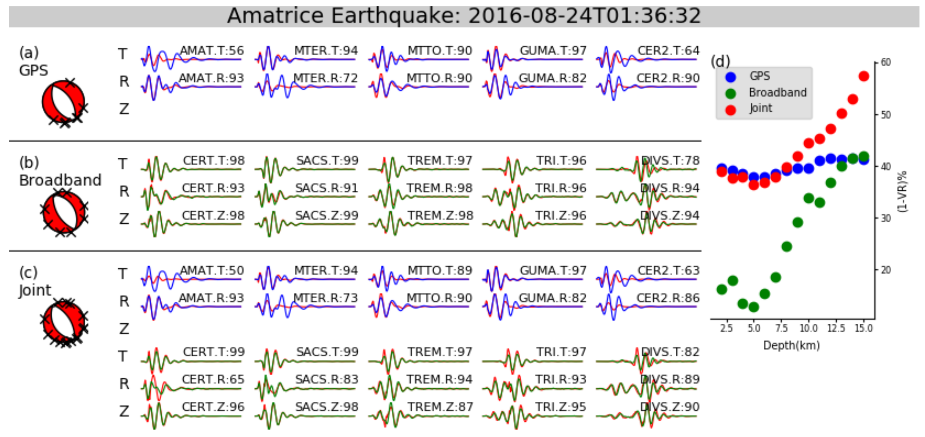
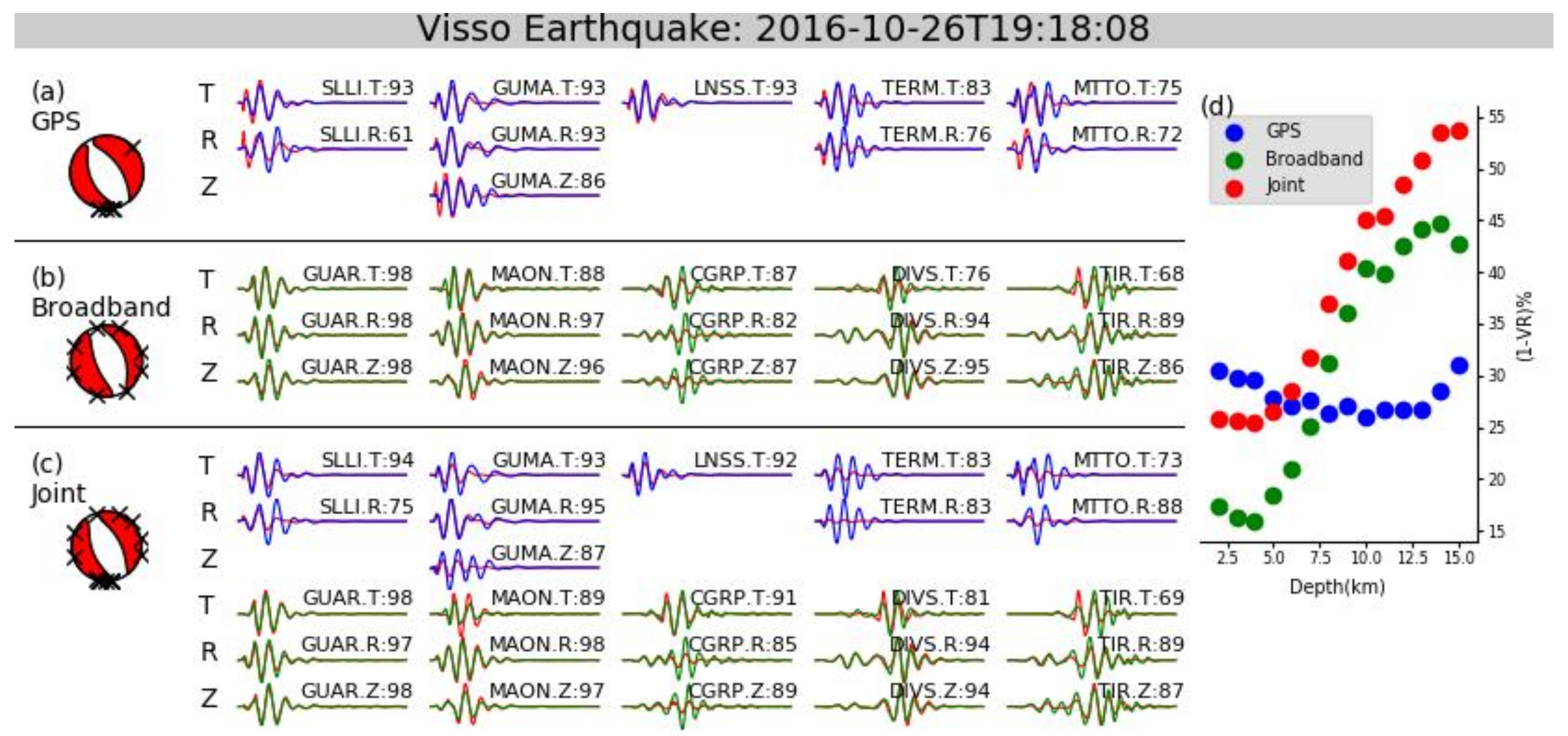
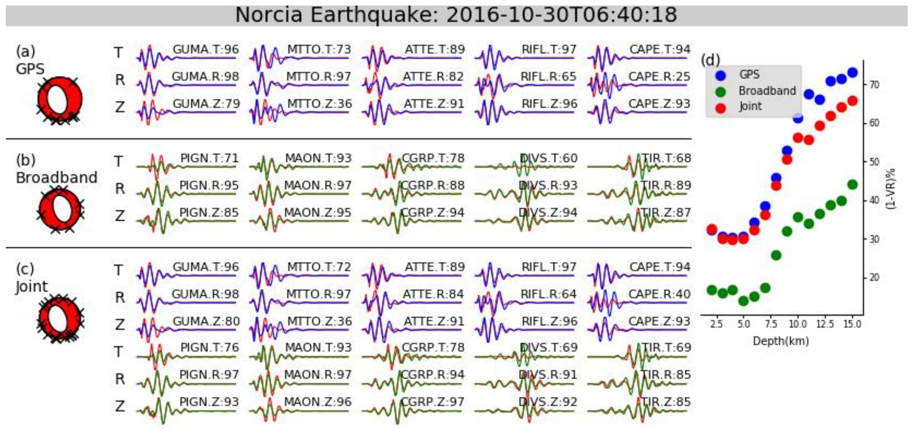
First, the high-rate GPS waveforms were used alone to determine the source parameters of the three events. The Amatrice earthquake was the second-largest event among the three mainshocks; the INGV reported a magnitude of Mw 6.1 for the event. Since the error in the vertical component is twice as large as that in either of the horizontal components, only the horizontal components of 7 stations were ultimately used for the inversion. A total of 13 of the 14 cross-correlation coefficients of the waveforms exceeded 0.6, and the VR of the inversion was 62% (Figure 4a). The Visso earthquake was the smallest of the three events, and the INGV reported a magnitude of Mw 5.9 for the event. The peak ground displacements at some of the stations were nearly equivalent to the GPS noise level, and thus, fewer waveforms recorded seismic signals with good signal-to-noise ratios. A total of 14 waveforms from 6 stations were used in the inversion, and the cross-correlation coefficients of 12 of those waveforms exceeded 0.6. The VR of the inversion was 74% (Figure 5a). The Norcia earthquake exhibited the largest magnitude of the three events. Consequently, the signal-to-noise ratios of the records from this event were much higher than those from the other two events. We chose 27 components from 11 stations to use for the inversion. The cross-correlation coefficients of 12 of those waveforms exceeded 0.6, and the VR of the inversion was 69.6% (Figure 6a). Notably, the waveforms sourced from this event and recorded by station RIFP at an epicentral distance of approximately 9 km could not be effectively fitted in the inversion, although the station exhibited a good data quality. Given that station RIFP is located along the strike of the fault and since the fault length of the Norcia earthquake is estimated to be more than 20 km, we infer that this station might be located upon the fault. Unfortunately, the movement along this fault recorded by station RIFP cannot be effectively described using a point-source model. Therefore, this station was excluded from the inversion.
Second, the source parameters were determined using unclipped broadband seismograms at epicentral distances of 100~600 km for a comparison with the results obtained above. Since the sensitivity of a broadband seismometer is much higher than that of a high-rate GPS instrument, the observed seismograms were more effectively fitted by the synthetic seismograms (Figure 4b, Figure 5b and Figure 6b). Most of the cross-correlation coefficients among the seismograms exceeded 0.8, and the VRs of the three inversions were all greater than 80%. The results for the Amatrice and Norcia earthquakes obtained using both high-rate GPS and broadband seismicity data were basically in agreement, except for the dip angles (Table 3). Zheng et al. [53] performed moment tensor inversion for the Mw 7.2 El Mayor-Cucapah earthquake using near-field high-rate GPS data, and the dip angle they obtained differed from the GCMT result by approximately 20°. Furthermore, upon calculating the misfit when the dip angle changes from 50° to 80°, they found little variation in the misfit. Therefore, they inferred that the dip angle is difficult to resolve using near-field data alone. This conclusion may explain the differences in dip angle we obtained. The inversion results using the two types of data for the Visso earthquake are quite different (Table 3). Considering the smaller magnitude of this event and the smaller number of GPS stations used in the inversion, the difference in the results obtained using high-rate GPS data might have been caused by the poor observation quality and poor azimuthal coverage. The VRs were calculated at depths from 2 to 15 km at an interval of 1 km to find the best fitted focal depth (Figure 4d, Figure 5d and Figure 6d). Within the depth range of 2~15 km, the VRs of the inversion results for the Amatrice, Visso and Norcia events using high-rate GPS data ranged from 58.5% to 62.2%, from 69.0% to 74.0% and from 26.8% to 69.6%, respectively. However, the corresponding ranges of VRs of the inversion results using broadband seismic data were 58.0~87.1%, 55.2~84.0% and 56.0~83.2%. For the smaller-magnitude Amatrice and Visso earthquakes, the VRs of the inversion results using high-rate GPS varied little at different depths, while the VR changes were more significant when the broadband seismograms were utilized. Therefore, the inversion results and constraints on the focal depths are more affected by noise in the GPS observations as the magnitude decreases.
Finally, a joint inversion was performed using high-rate GPS waveforms and broadband seismic data (Table 3, Figure 4c, Figure 5c and Figure 6c). The results were basically consistent with those obtained using broadband seismograms alone except for differences in the dip angles. For the Visso earthquake, the deviation in the results obtained using high-rate GPS data was corrected in the joint inversion. Due to the influence of noise in the GPS observations, the VRs of the inversions were smaller than those utilizing only broadband seismograms, but their variations at different depths were more obvious than those obtained using only high-rate GPS data.
4. Discussion
4.1. Sparce Network Tests
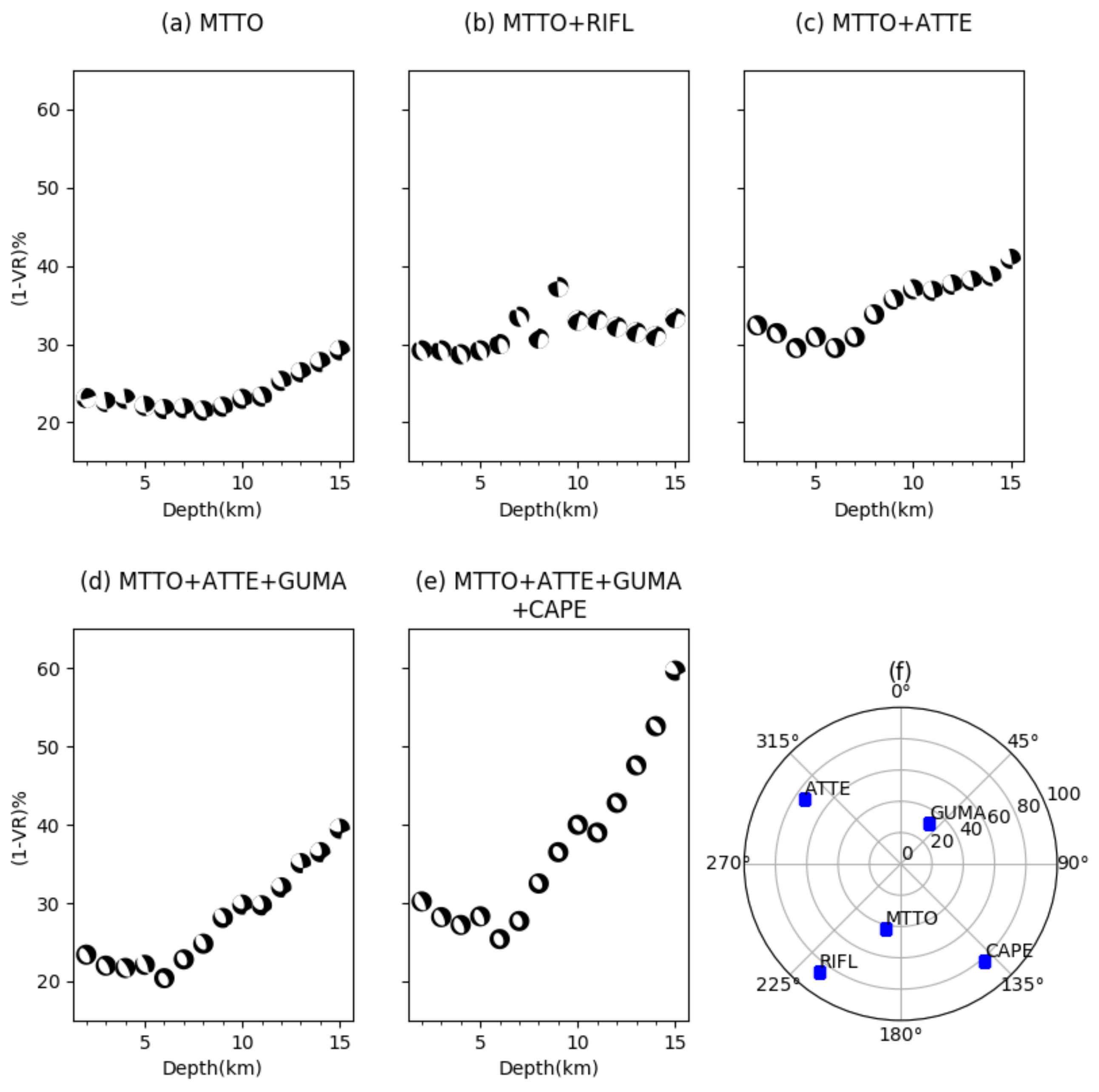
For the inversions in the previous chapter, we attempted to utilize as much high-rate GPS data as possible to make the results more reliable. Although multi-station data are generally used for waveform inversions to estimate the source parameters, focal mechanism solutions can also be obtained using waveform data from only one or two stations and the number of stations used and the network geometry can influence the quality of the inverted source parameters [57]. This is critical when source parameters need to be estimated at real time with limited data available or analyzing earthquakes occurring in locales where dense station network is not available, e.g., the Himalayan region. Dreger and Helmberger [49] suggested that single-station data are adequate for waveform inversion. Tan et al. [51] developed a new technique based on the CAP method to retrieve the source parameters of small seismic events using as few as two stations. Kumar et al. [58] analyzed two earthquakes in the Himalayan region and discovered that the solutions estimated using both multi-station and single-station data sets have nearly identical focal mechanism parameters. Guo et al. [54] performed sparse network tests using high-rate GPS velocity records from the El Mayor-Cucapah earthquake and obtained robust source parameters with an acceptable bias using as few as three stations. However, their GPS stations were all located to the northwest of the epicenter of the El Mayor-Cucapah earthquake, and thus, the stations they used in their tests show limited azimuthal coverage. To further understand the capabilities of high-rate GPS waveforms in a sparse network, we consider the Norcia earthquake, which has a better station coverage, and perform several tests with a limited number of stations (Table 4).
The source parameters obtained using a single GPS station differed considerably from the INGV results. The inversion result for station MTTO (Test 1, Figure 7a) is given as an example. When the number of stations is increased to two, the bias in the inversion result becomes acceptable. We present the inversion results from when station MTTO was used together with station RIFL (Test 2, Figure 7b) and station ATTE (Test 3, Figure 7c). The results of Test 2 and Test 3 are similar except for the dip angle, which can be explained as demonstrated above, but their VRs behave differently at different depths. The VR of Test 2 changed less than that of Test 3, and there are several discontinuities and local minima along the curve for the former. Since the stations used in Test 2 (MTTO and RIFL) are located closely within a narrow azimuthal range and since stations MTTO and ATTE are more distant from each other (and, therefore, have a clearly different azimuthal coverage), we infer that better azimuthal coverage and larger distance between two stations can provide better constraints on the inversion results. Therefore, in the following tests, we deliberately choose stations with better azimuthal coverage. The results of tests using three and four stations (Test 4 and Test 5, Figure 7d,e) are more similar to the results obtained previously. As the number of stations increases, the changes in the VR become more obvious at different depths, and the focal mechanisms obtained at different depths become more stable. The proportions of non-DC components in the moment tensors obtained for Test 4 and Test 5 are also more similar to the results presented in the previous chapter.
Our test demonstrates that a reasonable focal mechanism can be obtained using three-component waveforms from as few as two or three high-rate GPS stations. In addition, rather than the number of stations, the azimuthal coverage should be considered first to provide better constraints on the focal mechanism and focal depth.
4.2. Source Parameters
Previous studies employed high-rate GPS waveform data primarily for the study of large earthquakes [16,53,59,60]. The three earthquakes we investigated were all moderate-magnitude events; accordingly, the high-rate GPS observations recorded during those events were not as good as those from larger earthquakes. We retrieved the dynamic displacements of the three earthquakes from near-field high-rate GPS recordings through kinematic PPP analysis. In addition, a regional spatial filter was applied to reduce the CMEs. The results were then employed for focal mechanism inversions, and the synthetic waveforms fit relatively well with the observations. The source parameters of the Norcia and Amatrice earthquakes obtained using high-rate GPS data were more consistent with results provided by the INGV, except for the dip angle, which is difficult to resolve using near-field data alone. By comparing the results obtained using high-rate GPS data with those obtained using unclipped broadband seismic data, we observe that the resolution of the misfit in the focal depth was obviously weaker for the Amatrice and Visso earthquakes. Moreover, the source parameters of Visso earthquake is more different from other results. Considering the smaller magnitudes of these two events, we believe that these properties were mainly caused by the weaker recorded signals during the two events, i.e., the results were more affected by noise. We conclude that the near-field long-period waveform observed by high-rate GPS can act as a complement to clipped broadband seismograms in source parameter inversions. Through the joint inversion of high-rate GPS waveform data and broadband seismic data, the impacts of noise on the GPS observations are weakened, and the final results are more reliable.
The results of the sparse network tests indicate that reasonable focal mechanisms can be obtained using as few as two to three high-rate GPS stations. Since high-rate GPS data can be streamed in real time without clipping, tilting and long-period drift problems, near-field long-period signal can be obtained before the destructive surface wave propagates and attenuates to be unclippedly recorded by broadband seismometers or corrections for the strong motion data are made. Early obtaining of such signal can, therefore, help to quickly estimate the intensity and extent of earthquake disasters and launch tactical rescue operations. A rapidly inverted focal mechanism can provide important a priori information for subsequent inversions of the slip distribution and rupture process, especially for earthquakes such as the 2013 Lushan earthquake in China, which occurred along blind faults [61]. So, we conclude that high-rate GPS waveform data has the potential to be applied in rapid inversion and real-time monitoring of focal mechanisms in moderate-magnitude earthquakes to enhance the ability and reliability of existing earthquake monitoring or early warning networks in earthquakes with magnitude down to Mw 6. For well-observed moderate-magnitude earthquakes similar to the Norcia earthquake, reliable and rapid focal mechanisms can be obtained using a few high-rate GPS stations individually. For smaller-magnitude events, such as the Amatrice and Visso earthquakes, the epicentral distances of the stations should be considered, as the recorded waveforms may be more greatly affected by the background noise. The results obtained by joint inversions with broadband seismic data are more reliable in such situations.
In this work, the epicentral locations, which are required to calculate the Green’s functions, are assumed to be known a priori. However, if near-field GPS data are utilized for a rapid moment tensor inversion, the epicentral locations should be calculated beforehand with either seismic data or high-rate GPS data. However, due to high levels of background noise and the weak amplitudes of P-wave first arrivals, very few studies using high-rate GPS data have reported the identification of P waves, which is necessary for earthquake location determination [25]. With the development of high-rate GNSS data processing techniques [19] and multi-GNSS techniques [62], the precision of high-rate GPS data is gradually improving. Hopefully, high-rate GPS or multi-GNSS data can be independently utilized for earthquake early warning systems and for fast source modeling. However, although high-rate GPS networks can provide data with higher signal-to-noise ratios from larger earthquakes, larger earthquakes might violate the point-source assumption since we are employing near-field data. Therefore, a multiple CMT source model or a finite fault model might be required to better understand the observed signal from larger events. In this work, we didn’t apply extra weighting strategy for the GPS and broadband data in the joint inversions. However, the characteristics of these two types of data are quite different. Further investigations are needed with regard to the weighting of these two types of data in joint inversions.
4.3. Seismogenic Tectonics
According to our inversion results, the moment tensor solutions of the Amatrice and Visso earthquakes are almost purely DC, but the Norcia earthquake seems to require a large compensated linear vector dipole (CLVD) component (Table 3). The DC source model is based on the assumption that earthquakes are caused by shear faulting, for which the equivalent force system in an isotropic medium is a pair of force couples with no net torque [63]. Though the non-DC component in a moment tensor solution can also be ascribed to modeling errors introduced by the point-source assumption [41] and by small-scale heterogeneities in the crust [64], the large CLVD component in the Norcia earthquake is also evidenced by the results published by different institutions (Table 3) with similar proportions of approximately 30%. Therefore, we infer that some non-DC processes occurred during the Norcia earthquake and should, therefore, be considered.
Frohlich [65] demonstrated that a CLVD component in a moment tensor represents the superposition of DC ruptures along different faults. A similar phenomenon was observed within the 2016 Kumamoto sequence in Japan, in which significant non-DC components within the reported seismic focal mechanisms were due to the simultaneous occurrence of both strike-slip and normal dip-slip along distinct segments [66]. The Mw 6.5 Norcia earthquake, which occurred on 30 October, was spatially located in between the preceding mainshocks. It ruptured along the northern part of the Mount Vettore fault, the southern portion of which was only partially activated during the 24 August earthquake [8] and was accompanied by numerous aftershocks [13]. Associated slip distribution models all demonstrate a maximum slip exceeding 2.5 m and a concentrated patch of slip located at depths of 0~7 km [8,12,13,14] corresponding to observed surface fractures [67]. Cheloni et al. [8] observed large displacement residuals reaching up to ~10 cm within interferograms after jointly inverting the slip along the two segments of the MGVB fault system using GPS and InSAR data. Two different hypotheses were proposed to explain this phenomenon: (1) a NE-dipping normal fault antithetic to the MGVB fault system and (2) a preexisting compressional low-angle structure. The results of both models fit the observed data better than the results of the original MGVB fault system model. The retrieved slip on the additional dislocation is equivalent to a Mw 6.1~6.2 event. The relocated aftershock distribution [13] also suggests the presence of a set of synthetic and antithetic structures in this area. Therefore, we suggest that the large CLVD components in our moment tensor solutions derived from high-rate GPS and broadband seismic data support the presence of an additional dislocation in the Norcia earthquake, and our results reflect a more complex deformation pattern associated with this event.
5. Conclusions
The dynamic displacements of three moderate-magnitude earthquakes within the 2016 central Italy seismic sequence are retrieved from high-rate GPS records using kinematic PPP analysis. The high-rate GPS data provides waveforms in the epicentral area, where broadband seismograms are mostly clipped due to the strong shaking. The source parameters are estimated using high-rate GPS waveforms and unclipped broadband seismograms both independently and jointly. The results show that the moment magnitudes of the Amatrice, Visso, and Norcia events are Mw 6.1, Mw 5.9 and Mw 6.5, respectively, and the focal mechanisms for the three events are very similar. The moment tensor of the Norcia earthquake contains a significant proportion (30%) of a CLVD component, which indicates a more complicated fault rupture process. Our work demonstrates that the source parameters of moderate-magnitude earthquakes can be rapidly obtained by using high-rate GPS data in a waveform inversion. When the event magnitude is small, constraints on focal depth are affected by the background noise in GPS observations. In regions with sparse networks, reasonable focal mechanisms can be obtained using three-component waveforms from as few as two or three high-rate GPS stations. Thus, high-rate GPS waveform observations can act as a complement to clipped near-field long-period seismic waveform signals caused by the strong motion in source parameter inversions. Thus, it can effectively improve our understanding of moderate-magnitude tectonic earthquakes. Additionally, it has the potential to be applied in rapid inversion and real-time monitoring of focal mechanisms in moderate-magnitude earthquakes to enhance the ability and reliability of existing earthquake monitoring or early warning networks in earthquakes with magnitude down to Mw 6.
Supplementary Materials
The following are available online at https://www.mdpi.com/2072-4292/10/4/512/s1, Figures S1–S3, transverse, radial and vertical components of GPS displacement time series obtained in the Amatrice earthquake, the Visso earthquake and the Norcia earthquake, respectively. Figure S4, RMS histogram distributions on three components calculated in a 10 s time window before the earthquake origin time for all the used GPS data.
Acknowledgments
Author Contributions
Shuhan Zhong designed the study, performed the experiments, wrote and revised the manuscript; Caijun Xu designed the study, analyzed the experimental results and revised the manuscript; Lei Yi and Yanyan Li analyzed the experimental results and revised the manuscript.
Conflicts of Interest
The authors declare no conflict of interest.
References
- Emergeo Working Group. Coseismic effects of the 2016 Amatrice seismic sequence: First geological results. Ann. Geophys. 2016, 59. [Google Scholar] [CrossRef]
- Amato, A.; Azzara, R.; Chiarabba, C.; Cimini, G.B.; Cocco, M.; Di Bona, M.; Margheriti, L.; Mazza, S.; Mele, F.; Selvaggi, G.; et al. The 1997 Umbria-Marche, Italy, Earthquake Sequence: A first look at the main shocks and aftershocks. Geophys. Res. Lett. 1998, 25, 2861–2864. [Google Scholar] [CrossRef]
- Chiarabba, C.; Amato, A.; Anselmi, M.; Baccheschi, P.; Bianchi, I.; Cattaneo, M.; Cecere, G.; Chiaraluce, L.; Ciaccio, M.G.; De Gori, P.; et al. The 2009 L’Aquila (central Italy) MW6.3 earthquake: Main shock and aftershocks. Geophys. Res. Lett. 2009, 36. [Google Scholar] [CrossRef]
- Frepoli, A.; Amato, A. Contemporaneous extension and compression in the Northern Apennines from earthquake fault-plane solutions. Geophys. J. Int. 1997, 129, 368–388. [Google Scholar] [CrossRef]
- Akinci, A.; Galadini, F.; Pantosti, D.; Petersen, M.; Malagnini, L.; Perkins, D. Effect of Time Dependence on Probabilistic Seismic-Hazard Maps and Deaggregation for the Central Apennines, Italy. Bull. Seismol. Soc. Am. 2009, 99, 585–610. [Google Scholar] [CrossRef] [Green Version]
- Tinti, E.; Scognamiglio, L.; Michelini, A.; Cocco, M. Slip heterogeneity and directivity of the ML 6.0, 2016, Amatrice earthquake estimated with rapid finite-fault inversion. Geophys. Res. Lett. 2016, 43, 10745–10752. [Google Scholar] [CrossRef]
- Lavecchia, G.; Castaldo, R.; de Nardis, R.; De Novellis, V.; Ferrarini, F.; Pepe, S.; Brozzetti, F.; Solaro, G.; Cirillo, D.; Bonano, M.; et al. Ground deformation and source geometry of the 24 August 2016 Amatrice earthquake (Central Italy) investigated through analytical and numerical modeling of DInSAR measurements and structural-geological data. Geophys. Res. Lett. 2016, 43, 12389–12398. [Google Scholar] [CrossRef]
- Cheloni, D.; De Novellis, V.; Albano, M.; Antonioli, A.; Anzidei, M.; Atzori, S.; Avallone, A.; Bignami, C.; Bonano, M.; Calcaterra, S.; et al. Geodetic model of the 2016 Central Italy earthquake sequence inferred from InSAR and GPS data. Geophys. Res. Lett. 2017, 44, 6778–6787. [Google Scholar] [CrossRef]
- USGS Earthquake Hazards Program. Available online: https://earthquake.usgs.gov/ (accessed on 30 October 2017).
- Global Centroid Moment Tensor. Available online: http://www.globalcmt.org/ (accessed on 10 September 2017).
- INGV Centro Nazionale Terremoti. Available online: http://cnt.rm.ingv.it/en (accessed on 28 August 2017).
- Liu, C.; Zheng, Y.; Xie, Z.; Xiong, X. Rupture features of the 2016 Mw 6.2 Norcia earthquake and its possible relationship with strong seismic hazards. Geophys. Res. Lett. 2017, 44, 1320–1328. [Google Scholar] [CrossRef]
- Chiaraluce, L.; Stefano, R.D.; Tinti, E.; Scognamiglio, L.; Michele, M.; Casarotti, E.; Cattaneo, M.; Gori, P.D.; Chiarabba, C.; Monachesi, G.; et al. The 2016 Central Italy Seismic Sequence: A First Look at the Mainshocks, Aftershocks, and Source Models. Seismol. Res. Lett. 2017, 88, 757–771. [Google Scholar] [CrossRef]
- Xu, G.; Xu, C.; Wen, Y.; Jiang, G. Source Parameters of the 2016–2017 Central Italy Earthquake Sequence from the Sentinel-1, ALOS-2 and GPS Data. Remote Sens. 2017, 9, 1182. [Google Scholar] [CrossRef]
- Zhang, J.; Hao, J.; Zhao, X.; Wang, S.; Zhao, L.; Wang, W.; Yao, Z. Restoration of clipped seismic waveforms using projection onto convex sets method. Sci. Rep. 2016, 6. [Google Scholar] [CrossRef] [PubMed]
- Niu, J.; Xu, C.; Yi, L. Detecting Multiple Surface Waves Excited by the 2011 Tohoku-Oki Earthquake from GEONET Observations. Bull. Seismol. Soc. Am. 2016, 106, 806–811. [Google Scholar] [CrossRef]
- Kelevitz, K.; Houlié, N.; Giardini, D.; Rothacher, M. Performance of High-Rate GPS Waveforms at Long Periods: Moment Tensor Inversion of the 2003 Mw 8.3 Tokachi-Oki. Bull. Seismol. Soc. Am. 2017, 107, 1891–1903. [Google Scholar] [CrossRef]
- Psimoulis, P.A.; Houlié, N.; Michel, C.; Meindl, M.; Rothacher, M. Long-period surface motion of the multipatch Mw 9.0 Tohoku-Oki earthquake. Geophys. J. Int. 2014, 199, 968–980. [Google Scholar] [CrossRef]
- Li, Y.; Xu, C.; Yi, L. Denoising effect of multiscale multiway analysis on high-rate GPS observations. GPS Solut. 2017, 21, 31–41. [Google Scholar] [CrossRef]
- Melgar, D.; LeVeque, R.J.; Dreger, D.S.; Allen, R.M. Kinematic rupture scenarios and synthetic displacement data: An example application to the Cascadia subduction zone. J. Geophys. Res. Solid Earth 2016, 121, 6658–6674. [Google Scholar] [CrossRef]
- Boore, D.M. Effect of Baseline Corrections on Displacements and Response Spectra for Several Recordings of the 1999 Chi-Chi, Taiwan, Earthquake. Bull. Seismol. Soc. Am. 2001, 91, 1199–1211. [Google Scholar] [CrossRef]
- Wang, R.; Schurr, B.; Milkereit, C.; Shao, Z.; Jin, M. An Improved Automatic Scheme for Empirical Baseline Correction of Digital Strong-Motion Records. Bull. Seismol. Soc. Am. 2011, 101, 2029–2044. [Google Scholar] [CrossRef]
- Wang, R.; Parolai, S.; Ge, M.; Jin, M.; Walter, T.R.; Zschau, J. The 2011 Mw 9.0 Tohoku Earthquake: Comparison of GPS and Strong-Motion Data. Bull. Seismol. Soc. Am. 2013, 103, 1336–1347. [Google Scholar] [CrossRef]
- Genrich, J.F.; Bock, Y. Instantaneous geodetic positioning with 10–50 Hz GPS measurements: Noise characteristics and implications for monitoring networks. J. Geophys. Res. 2006, 111. [Google Scholar] [CrossRef]
- Avallone, A.; Marzario, M.; Cirella, A.; Piatanesi, A.; Rovelli, A.; Di Alessandro, C.; D’Anastasio, E.; D’Agostino, N.; Giuliani, R.; Mattone, M. Very high rate (10 Hz) GPS seismology for moderate-magnitude earthquakes: The case of the Mw 6.3 L’Aquila (central Italy) event. J. Geophys. Res. 2011, 116. [Google Scholar] [CrossRef]
- Incorporated Research Institutions for Seismology. Available online: http://www.iris.edu/ (accessed on 15 August 2017).
- Istituto Nazionale di Geofisica e Vulcanologia (INGV). INGV RING Working Group (2016), Rete Integrata Nazionale GPS (RING). Available online: https://doi.org/10.13127/RING (accessed on 30 October 2017).
- Davis, J.P.; Smalley, R. Love wave dispersion in central North America determined using absolute displacement seismograms from high-rate GPS. J. Geophys. Res. 2009, 114. [Google Scholar] [CrossRef]
- Michel, C.; Kelevitz, K.; Houlié, N.; Edwards, B.; Psimoulis, P.; Su, Z.; Clinton, J.; Giardini, D. The Potential of High-Rate GPS for Strong Ground Motion Assessment. Bull. Seismol. Soc. Am. 2017, 107, 1849–1859. [Google Scholar] [CrossRef]
- Zumberge, J.F.; Heflin, M.B.; Jefferson, D.C.; Watkins, M.M.; Webb, F.H. Precise point positioning for the efficient and robust analysis of GPS data from large networks. J. Geophys. Res. 1997, 102, 5005–5017. [Google Scholar] [CrossRef]
- Bertiger, W.; Desai, S.D.; Haines, B.; Harvey, N.; Moore, A.W.; Owen, S.; Weiss, J.P. Single receiver phase ambiguity resolution with GPS data. J. Geodesy 2010, 84, 327–337. [Google Scholar] [CrossRef]
- Herring, T.A.; King, R.W.; McClusky, S.C. Introduction to Gamit/Globk. 2010. Avilable online: http://www-gpsg.mit.edu/~simon/gtgk/docs.htm (accessed on 30 October 2017).
- Avallone, A.; Latorre, D.; Serpelloni, E.; Cavaliere, A.; Herrero, A.; Cecere, G.; D’Agostino, N.; D’Ambrosio, C.; Devoti, R.; Giuliani, R.; et al. Coseismic displacement waveforms for the 2016 August 24 Mw 6.0 Amatrice earthquake (central Italy) carried out from High-Rate GPS data. Ann. Geophys. 2016, 59. [Google Scholar] [CrossRef]
- Boehm, J.; Werl, B.; Schuh, H. Troposphere mapping functions for GPS and very long baseline interferometry from European Centre for Medium-Range Weather Forecasts operational analysis data. J. Geophys. Res. 2006, 111. [Google Scholar] [CrossRef]
- Kedar, S.; Hajj, G.A.; Wilson, B.D.; Heflin, M.B. The effect of the second order GPS ionospheric correction on receiver positions. Geophys. Res. Lett. 2003, 30. [Google Scholar] [CrossRef]
- Wdowinski, S.; Bock, Y.; Zhang, J.; Fang, P.; Genrich, J. Southern California permanent GPS geodetic array: Spatial filtering of daily positions for estimating coseismic and postseismic displacements induced by the 1992 Landers earthquake. J. Geophys. Res. 1997, 102, 18057–18070. [Google Scholar] [CrossRef]
- Nikolaidis, R. Observation of Geodetic and Seismic Deformation with the Global Positioning System. Ph.D. Thesis, University of California, San Diego, CA, USA, 2002. [Google Scholar]
- Jackson, D.A.; Chen, Y. Robust principal component analysis and outlier detection with ecological data. Environmetrics 2004, 15, 129–139. [Google Scholar] [CrossRef]
- He, X.; Hua, X.; Yu, K.; Xuan, W.; Lu, T.; Zhang, W.; Chen, X. Accuracy enhancement of GPS time series using principal component analysis and block spatial filtering. Adv. Space Res. 2015, 55, 1316–1327. [Google Scholar] [CrossRef]
- Dong, D.; Fang, P.; Bock, Y.; Webb, F.; Prawirodirdjo, L.; Kedar, S.; Jamason, P. Spatiotemporal filtering using principal component analysis and Karhunen-Loeve expansion approaches for regional GPS network analysis. J. Geophys. Res. 2006, 111. [Google Scholar] [CrossRef]
- Melgar, D.; Bock, Y.; Crowell, B.W. Real-time centroid moment tensor determination for large earthquakes from local and regional displacement records. Geophys. J. Int. 2012, 188, 703–718. [Google Scholar] [CrossRef]
- Crowell, B.W.; Bock, Y.; Melgar, D. Real-time inversion of GPS data for finite fault modeling and rapid hazard assessment. Geophys. Res. Lett. 2012, 39. [Google Scholar] [CrossRef]
- Ohta, Y.; Kobayashi, T.; Tsushima, H.; Miura, S.; Hino, R.; Takasu, T.; Fujimoto, H.; Iinuma, T.; Tachibana, K.; Demachi, T.; et al. Quasi real-time fault model estimation for near-field tsunami forecasting based on RTK-GPS analysis: Application to the 2011 Tohoku-Oki earthquake (Mw 9.0). J. Geophys. Res. 2012, 117. [Google Scholar] [CrossRef]
- Colombelli, S.; Allen, R.M.; Zollo, A. Application of real-time GPS to earthquake early warning in subduction and strike-slip environments. J. Geophys. Res. Solid Earth 2013, 118, 3448–3461. [Google Scholar] [CrossRef]
- Grapenthin, R.; Johanson, I.A.; Allen, R.M. Operational real-time GPS-enhanced earthquake early warning. J. Geophys. Res. Solid Earth 2014, 119, 7944–7965. [Google Scholar] [CrossRef]
- Minson, S.E.; Murray, J.R.; Langbein, J.O.; Gomberg, J.S. Real-time inversions for finite fault slip models and rupture geometry based on high-rate GPS data. J. Geophys. Res. Solid Earth 2014, 119, 3201–3231. [Google Scholar] [CrossRef]
- Zhu, L.; Ben-Zion, Y. Parametrization of general seismic potency and moment tensors for source inversion of seismic waveform data. Geophys. J. Int. 2013, 194, 839–843. [Google Scholar] [CrossRef]
- Zhao, L.-S.; Helmberger, D.V. Source estimation from broadband regional seismograms. Bull. Seismol. Soc. Am. 1994, 84, 91–104. [Google Scholar]
- Dreger, D.S.; Helmberger, D.V. Determination of source parameters at regional distances with three-component sparse network data. J. Geophys. Res. 1993, 98, 8107–8125. [Google Scholar] [CrossRef]
- Zhu, L.; Helmberger, D.V. Advancement in source estimation techniques using broadband regional seismograms. Bull. Seismol. Soc. Am. 1996, 86, 1634–1641. [Google Scholar]
- Tan, Y.; Zhu, L.; Helmberger, D.V.; Saikia, C.K. Locating and modeling regional earthquakes with two stations. J. Geophys. Res. 2006, 111. [Google Scholar] [CrossRef]
- Zhao, L.; Luo, Y.; Liu, T.-Y.; Luo, Y.-J. Earthquake Focal Mechanisms in Yunnan and their Inference on the Regional Stress Field. Bull. Seismol. Soc. Am. 2013, 103, 2498–2507. [Google Scholar] [CrossRef]
- Zheng, Y.; Li, J.; Xie, Z.; Ritzwoller, M.H. 5Hz GPS seismology of the El Mayor—Cucapah earthquake: Estimating the earthquake focal mechanism. Geophys. J. Int. 2012, 190, 1723–1732. [Google Scholar] [CrossRef]
- Guo, A.; Ni, S.; Chen, W.; Freymueller, J.T.; Shen, Z. Rapid earthquake focal mechanism inversion using high-rate GPS velometers in sparse network. Sci. China Earth Sci. 2015, 58, 1970–1981. [Google Scholar] [CrossRef]
- Herrmann, R.B.; Malagnini, L.; Munafò, I. Regional Moment Tensors of the 2009 L’Aquila Earthquake Sequence. Bull. Seismol. Soc. Am. 2011, 101, 975–993. [Google Scholar] [CrossRef]
- Zhu, L.; Rivera, L.A. A note on the dynamic and static displacements from a point source in multilayered media. Geophys. J. Int. 2002, 148, 619–627. [Google Scholar] [CrossRef]
- Zhang, Y.; Dalguer, L.A.; Song, S.G.; Clinton, J.; Giardini, D. Evaluating the effect of network density and geometric distribution on kinematic source inversion models. Geophys. J. Int. 2015, 200, 1–16. [Google Scholar] [CrossRef]
- Kumar, R.; Gupta, S.C.; Kumar, A. Determination and identification of focal mechanism solutions for Himalayan earthquakes from waveform inversion employing ISOLA software. Nat. Hazards 2015, 76, 1163–1181. [Google Scholar] [CrossRef]
- Delouis, B.; Nocquet, J.-M.; Vallée, M. Slip distribution of the February 27, 2010 Mw = 8.8 Maule Earthquake, central Chile, from static and high-rate GPS, InSAR, and broadband teleseismic data. Geophys. Res. Lett. 2010, 37. [Google Scholar] [CrossRef]
- Yue, H.; Lay, T. Inversion of high-rate (1 sps) GPS data for rupture process of the 11 March 2011 Tohoku earthquake (Mw 9.1). Geophys. Res. Lett. 2011, 38. [Google Scholar] [CrossRef]
- Xu, X.W.; Wen, X.Z.; Han, Z.J.; Chen, G.H.; Li, C.Y.; Zheng, W.J.; Zhang, S.M.; Ren, Z.Q.; Xu, C.; Tan, X.B.; et al. Lushan MS7.0 earthquake: A blind reserve-fault event. Chin. Sci. Bull. 2013, 58, 3437–3443. [Google Scholar] [CrossRef]
- Geng, J.; Jiang, P.; Liu, J. Integrating GPS with GLONASS for high-rate seismogeodesy. Geophys. Res. Lett. 2017, 44, 3139–3146. [Google Scholar] [CrossRef]
- Julian, B.R.; Miller, A.D.; Foulger, G.R. Non-double-couple earthquakes 1. Theory. Rev. Geophys. 1998, 36, 525–549. [Google Scholar] [CrossRef]
- Zhu, L.; Zhou, X. Seismic moment tensor inversion using 3D velocity model and its application to the 2013 Lushan earthquake sequence. Phys. Chem. Earth Parts A B C 2016, 95, 10–18. [Google Scholar] [CrossRef]
- Frohlich, C. Characteristics of well-determined non-double-couple earthquakes in the Harvard CMT catalog. Phys. Earth Planet. Inter. 1995, 91, 213–228. [Google Scholar] [CrossRef]
- Himematsu, Y.; Furuya, M. Fault source model for the 2016 Kumamoto earthquake sequence based on ALOS-2/PALSAR-2 pixel-offset data: Evidence for dynamic slip partitioning. Earth Planets Space 2016, 68. [Google Scholar] [CrossRef]
- Stewart, J. Engineering Reconnaissance Following the October 2016 Central Italy Earthquakes Version 2. GEER Association, 2017. Available online: https://doi.org/10.18118/g6hs39 (accessed on 30 October 2017).
- Wessel, P.; Smith, W.H.F.; Scharroo, R.; Luis, J.; Wobbe, F. Generic Mapping Tools: Improved Version Released. Eos Trans. AGU 2013, 94, 409–410. [Google Scholar] [CrossRef]
- Hunter, J.D. Matplotlib: A 2D Graphics Environment. Comput. Sci. Eng. 2007, 9, 90–95. [Google Scholar] [CrossRef]
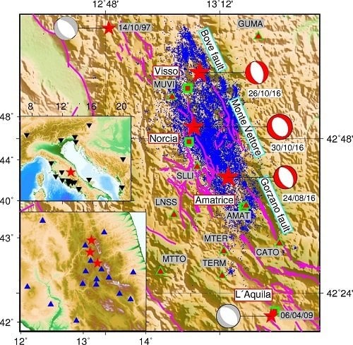
Figure 1.
Map of the study area. Red stars, the epicentral location of the three mainshocks together with historical events. Beachballs, Istituto Nazionale di Geofisica e Vulcanologia (INGV) focal mechanisms of the three mainshocks and historical events, respectively. Blue dots, aftershock locations. Magenta lines, main fault extents in this area. Triangles and inversed triangles, high-rate Global Positioning System (GPS) stations and broadband seismometers used in this work.
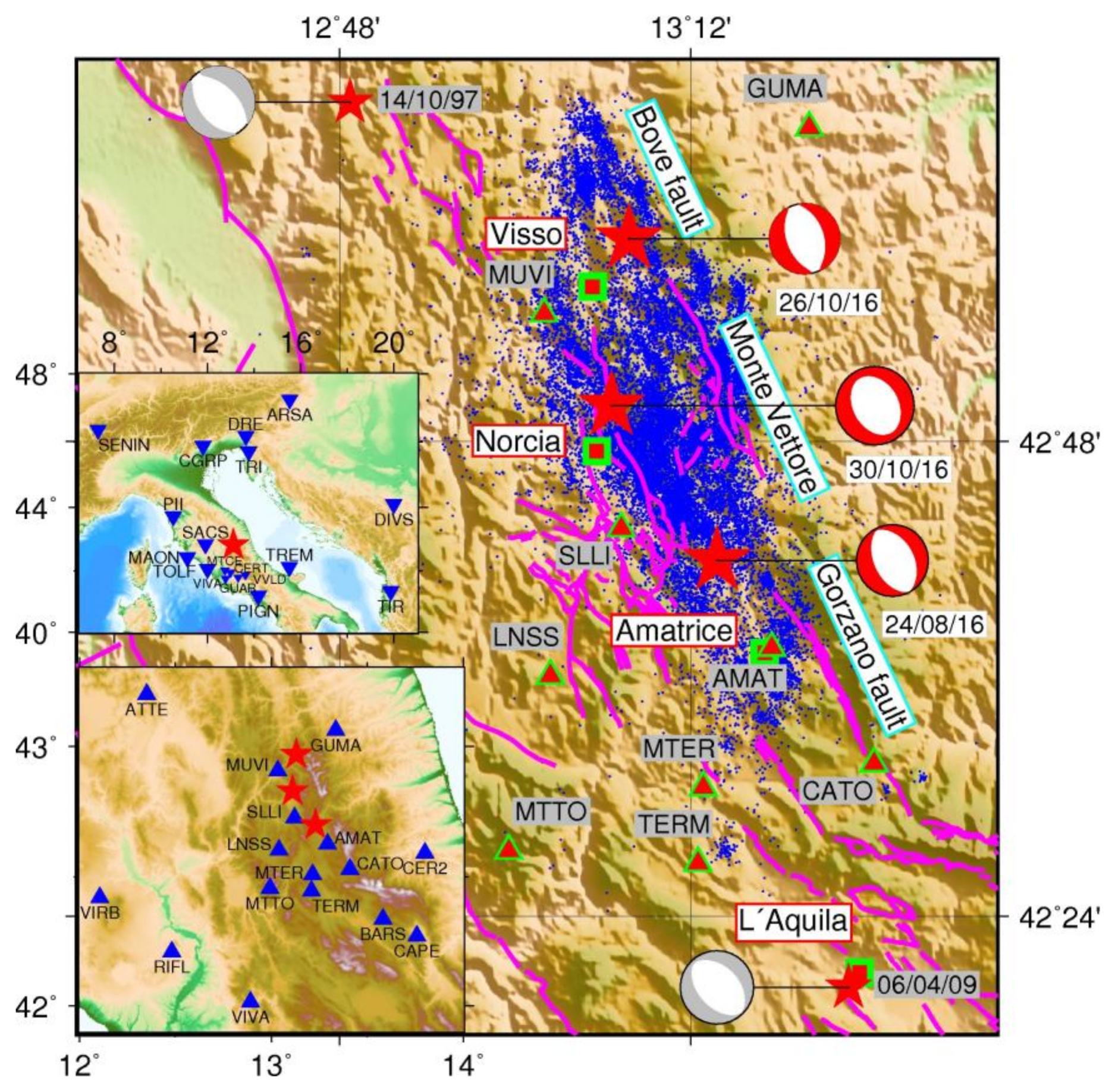
Figure 2.
Distribution of clipped seismometers associated with the three mainshocks and the distribution of high-rate GPS stations. Blue star, dashed circle, and dots represent epicenter, 100 km epicentral distance area and clipped broadband seismometers in the Amatrice earthquake. Green star, dashed circle, and triangles represent epicenter, 100 km epicentral distance area and clipped broadband seismometers in the Visso earthquake. Red star, dashed circle, and squares represent epicenter, 100 km epicentral distance area and clipped broadband seismometers in the Norcia earthquake. Yellow squares, location of high-rate GPS stations.

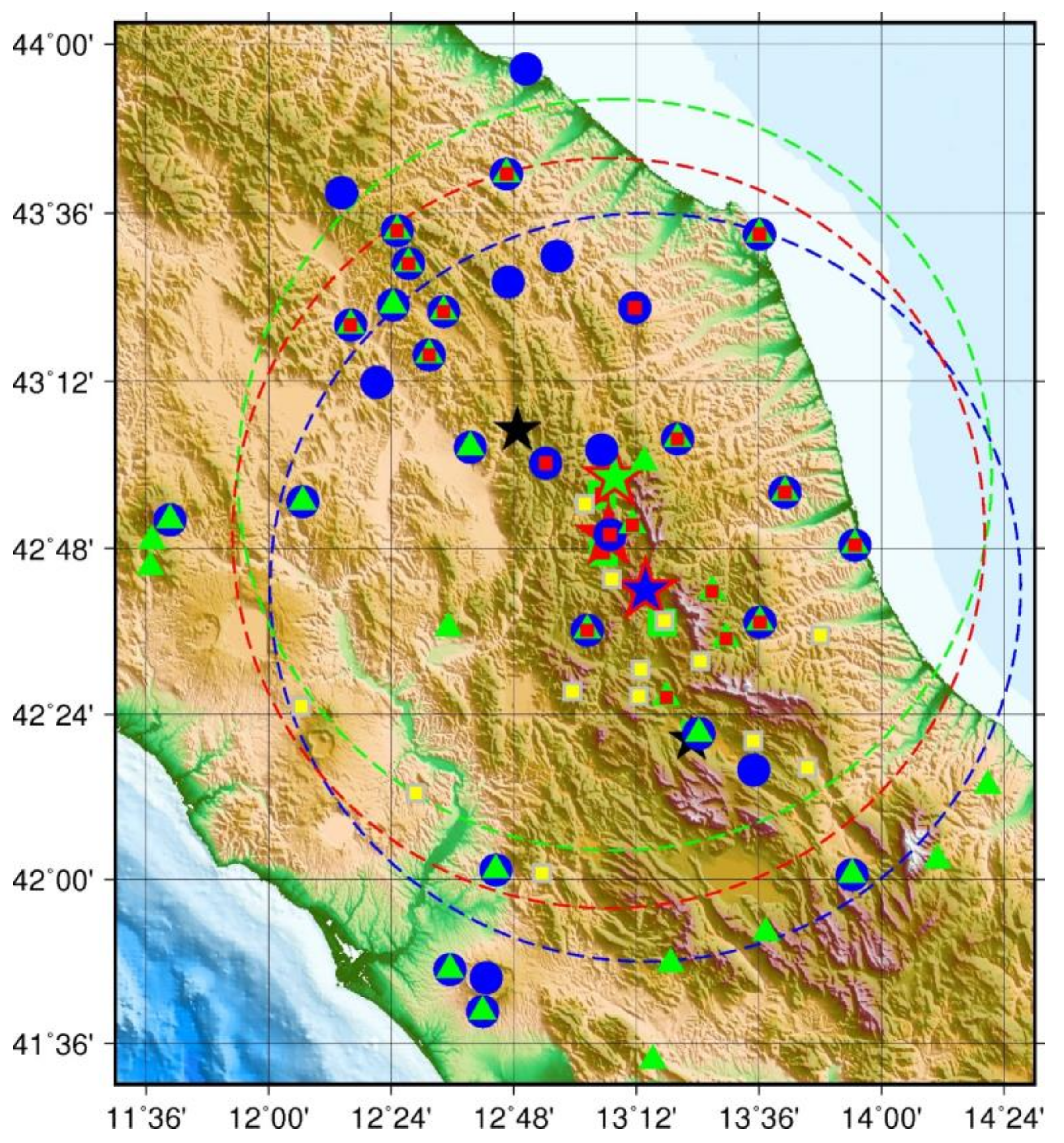
Figure 3.
Example of clipped three-component broadband seismograms and regional spatial filtering of GPS data. (a–c) Clipped three-component broadband seismograms in the Norcia earthquake recorded at the broadband seismometer at station CAFR, located about 120 km from the epicenter. (d) E-W displacement time series with common mode error, recorded at GPS station GUMA in the Visso earthquake; (e) Averaged common mode error extracted from GPS stations out of the epicentral area in the Visso earthquake; (f) E-W displacement time series of station GUMA in the Visso earthquake, with common mode error removed; (g) E-W velocity waveform of station GUMA in the Visso earthquake.

Figure 4.
Inversion results of the Amatrice Earthquake. (a–c), focal mechanisms and comparison between the observed and synthetic seismograms of the inversion using high-rate GPS data, broadband data and both of them, respectively. Blue and green lines in (a–c) are observed high-rate GPS and broadband waveforms, respectively. Red lines are synthetic seismograms. Crosses on the beachballs indicate the azimuths of the stations used in the inversions. Texts upon waveforms are station names, component names and the cross-correlation coefficients. (d) VRs of the inversions at depth from 2 km to 15 km. As space is limited, waveforms from only five GPS stations and five broadband stations are exhibited here.

Figure 5.
Inversion results of the Visso Earthquake. The representing scheme of the subplots is the same as Figure 4.
Figure 5.
Inversion results of the Visso Earthquake. The representing scheme of the subplots is the same as Figure 4.

Figure 6.
Inversion results of the Norcia Earthquake. The representing scheme of the subplots is the same as Figure 4.
Figure 6.
Inversion results of the Norcia Earthquake. The representing scheme of the subplots is the same as Figure 4.

Figure 7.
Results of the sparse network tests and the distribution of stations. (a–e) variance reductions (VRs) and focal mechanisms of the Norcia earthquake, obtained by different numbers of stations, at depth from 2 km to 15 km; (f) Azimuthal and epicentral distribution of stations used in the sparse network tests; the origin point is the epicenter of the Norcia earthquake.


Table 1.
High-rate GPS data processing strategy.
| Options | Values |
|---|---|
| Sampling rate | 10 Hz |
| Time span | Origin time ±3 min |
| Troposphere mapping function | VMF1 GRID |
| Troposphere parameter model | Random Walk 5×10⁻⁸ km/s |
| Troposphere delay gradient | 5×10⁻⁹ km/s0.5 |
| Ionosphere correction | CODE IONEX |
| Orbit and clock product | JPL Final |
| Stochastic model | White Noise 1×10⁻³ km |
Table 2.
Crustal velocity model.
| Thickness | |||
|---|---|---|---|
| 0.5 | 4.03 | 2.30 | 2.323 |
| 0.5 | 3.81 | 2.18 | 2.287 |
| 0.5 | 3.73 | 2.13 | 2.271 |
| 1 | 4.54 | 2.59 | 2.398 |
| 1 | 5.16 | 2.95 | 2.532 |
| 1 | 5.58 | 3.18 | 2.616 |
| 3 | 5.69 | 3.25 | 2.637 |
| 3 | 5.38 | 3.05 | 2.576 |
| 4 | 6.05 | 3.43 | 2.714 |
| 5 | 5.51 | 3.15 | 2.602 |
| 5 | 6.16 | 3.52 | 2.747 |
| 5 | 5.76 | 3.29 | 2.651 |
| 6 | 6.42 | 3.62 | 2.828 |
| 8 | 7.35 | 4.13 | 3.090 |
| - | 7.90 | 4.40 | 3.276 |
Table 3.
Source parameters of the three events using different types of data compared with published results [9,10,11].
| Event | Source | Moment (N·m) | Mw 1 | Strike (°) | Dip (°) | Rake (°) | Depth (km) | DC% | VR% |
|---|---|---|---|---|---|---|---|---|---|
| Amatrice | USGSW 2 | 2.45×10¹⁸ | 6.2 | 165 | 49 | −78 | 11.5 | 86 | - |
| GCMT | 2.48×10¹⁸ | 6.2 | 145 | 38 | −101 | 12 | 96 | ||
| INGV | 1.07×10¹⁸ | 6 | 155 | 49 | −87 | 5 | 98 | ||
| GPS | 2.21×10¹⁸ | 6.2 | 152 | 40 | −84 | 6 | 100 | 62.2 | |
| Broadband | 1.42×10¹⁸ | 6.1 | 148 | 55 | −90 | 5 | 100 | 87.1 | |
| Joint | 1.95×10¹⁸ | 6.13 | 146 | 37 | −90 | 6 | 100 | 63.2 | |
| Visso | USGSW | 1.84×10¹⁸ | 6.1 | 155 | 50 | −89 | 11.5 | 90 | - |
| GCMT | 1.61×10¹⁸ | 6.1 | 152 | 35 | −94 | 12 | 92 | ||
| INGV | 7.38×10¹⁷ | 5.9 | 159 | 47 | −93 | 6 | 96 | ||
| GPS | 2.79×10¹⁸ | 6.23 | 158 | 40 | −78 | 10 | 97 | 74 | |
| Broadband | 1.00×10¹⁸ | 5.93 | 158 | 55 | −90 | 4 | 91 | 84 | |
| Joint | 1.02×10¹⁸ | 5.94 | 161 | 44 | −82 | 4 | 90 | 74.5 | |
| Norcia | USGSW | 1.07×10¹⁹ | 6.6 | 162 | 27 | −84 | 15.5 | 82 | - |
| GCMT | 9.58×10¹⁸ | 6.6 | 154 | 37 | −96 | 12 | 85 | ||
| INGV | 7.07×10¹⁸ | 6.5 | 151 | 47 | −89 | 5 | 68 | ||
| GPS | 9.45×10¹⁸ | 6.58 | 165 | 32 | −90 | 4 | 66 | 69.6 | |
| Broadband | 8.07×10¹⁸ | 6.54 | 163 | 58 | −90 | 5 | 69 | 86 | |
| Joint | 8.19×10¹⁸ | 6.54 | 161 | 33 | −90 | 4 | 71 | 70.4 |
1 Moment magnitude; 2 The USGS W-phase moment tensor solution.
Table 4.
Results of the sparse network tests, compared with the solution obtained previously and the INGV results.
Table 4.
Results of the sparse network tests, compared with the solution obtained previously and the INGV results.
| Test No. | Moment (N·m) | Mw | Strike (°) | Dip (°) | Rake (°) | Depth (km) | DC% | VR% |
|---|---|---|---|---|---|---|---|---|
| 1 | 7.31×10¹⁸ | 6.51 | 119 | 30 | −128 | 8 | 98 | 78.8 |
| 2 | 8.70×10¹⁸ | 6.56 | 161 | 56 | −80 | 4 | 99 | 71.3 |
| 3 | 9.60×10¹⁸ | 6.59 | 159 | 25 | −80 | 4 | 82 | 70.5 |
| 4 | 9.04×10¹⁸ | 6.57 | 159 | 33 | −82 | 6 | 66 | 79.6 |
| 5 | 9.80×10¹⁸ | 6.59 | 157 | 33 | −90 | 6 | 60 | 74.6 |
| GPS ALL | 9.45×10¹⁸ | 6.58 | 165 | 32 | −90 | 4 | 66 | 69.6 |
| INGV | 7.07×10¹⁸ | 6.5 | 151 | 47 | −89 | 5 | 68 | - |
© 2018 by the authors. Licensee MDPI, Basel, Switzerland. This article is an open access article distributed under the terms and conditions of the Creative Commons Attribution (CC BY) license (http://creativecommons.org/licenses/by/4.0/).
Share and Cite
MDPI and ACS Style
Zhong, S.; Xu, C.; Yi, L.; Li, Y. Focal Mechanisms of the 2016 Central Italy Earthquake Sequence Inferred from High-Rate GPS and Broadband Seismic Waveforms. Remote Sens. 2018, 10, 512. https://doi.org/10.3390/rs10040512
AMA Style
Zhong S, Xu C, Yi L, Li Y. Focal Mechanisms of the 2016 Central Italy Earthquake Sequence Inferred from High-Rate GPS and Broadband Seismic Waveforms. Remote Sensing. 2018; 10(4):512. https://doi.org/10.3390/rs10040512
Chicago/Turabian StyleZhong, Shuhan, Caijun Xu, Lei Yi, and Yanyan Li. 2018. "Focal Mechanisms of the 2016 Central Italy Earthquake Sequence Inferred from High-Rate GPS and Broadband Seismic Waveforms" Remote Sensing 10, no. 4: 512. https://doi.org/10.3390/rs10040512
Note that from the first issue of 2016, this journal uses article numbers instead of page numbers. See further details here.