Wind Gust Detection and Impact Prediction for Wind Turbines


1
Mechanical Engineering, Arizona State University, Tempe, AZ 85287, USA
2
National Center for Atmospheric Research, Boulder, CO 80305, USA
3
Data Science Group, SAP, 1101 W Washington St #401, Tempe, AZ 85281, USA
*
Author to whom correspondence should be addressed.
Remote Sens. 2018, 10(4), 514; https://doi.org/10.3390/rs10040514
Submission received: 25 January 2018
/
Revised: 17 March 2018
/
Accepted: 23 March 2018
/
Published: 25 March 2018
(This article belongs to the Special Issue Remote Sensing of Atmospheric Conditions for Wind Energy Applications)
Abstract
:Wind gusts on a scale from 100 m to 1000 m are studied due to their significant influence on wind turbine performance. A detecting and tracking algorithm is proposed to extract gusts from a wind field and track their movement. The algorithm utilizes the “peak over threshold method,” Moore-Neighbor tracing algorithm, and Taylor’s frozen turbulence hypothesis. The algorithm was implemented for a three-hour, two-dimensional wind field retrieved from the measurements of a coherent Doppler lidar. The Gaussian shape distribution of the gust spanwise deviation from the streamline was demonstrated. Size dependency of gust deviations is discussed, and an empirical power function is derived. A prediction model estimating the impact of gusts with respect to arrival time and the probability of arrival locations is introduced, in which the Gaussian plume model and random walk theory including size dependency are applied. The prediction model was tested and the results reveal that the prediction model can represent the spanwise deviation of the gusts and capture the effect of gust size. The prediction model was applied to a virtual wind turbine array, and estimates are given for which wind turbines would be impacted.
1. Introduction
Rapid changes of wind speed in the atmosphere, also called wind gusts, cause large fatigue loads on wind turbines. These loads reduce the lifetime of wind turbine components. Oscillations or ramping of the generated power can result in fast fluctuations of grid voltage and may pose additional burdens to the electric grid. Researchers have proposed adaptive and feed-forward control systems, which can adjust wind turbine settings for approaching winds [1,2,3,4]. A feed-forward control system requires accurate and fast gust detection system. Our purpose is to provide the information of wind gusts to the control systems.
There are a variety of gust detecting and tracking algorithms in the literature. The international standard IEC 61400-1 specifies standardization of several temporal gust models for wind turbine design. Branlard defined gusts as a short-term wind speed variation within a turbulent wind field [5,6]. Although different definitions exist, all suggest gusts invoke rapid wind speed changes. As many atmospheric sensors measure winds in relatively small volumes, changes in wind speed have been considered temporally. Temporal variations of wind speed can be converted to spatial variations using Taylor’s frozen turbulence hypothesis. Note that spatial variations in pressure on wind speed also damage buildings [7]. However, fewer studies directly measure spatial variations. The lack of such studies could be due to the limitation of the available instruments. Anemometers on met masts are the most common instruments for gust studies, but they are limited to measuring wind speed at fixed points. On the other hand, Doppler lidar can address this limitation. A long-range Doppler lidar can provide wind velocity field in a 3D domain up to 10 km with high temporal and spatial resolution.
The scale of a spatial gust is an important factor. Kelley et al. [8] and Chamorro et al. [9] studied the flow-structure interaction between wind turbines and atmospheric coherent structures with a scale ranging from the size of a wind turbine rotor to the thickness of the atmospheric boundary layer. They found that structures primarily in that range have a high correlation with the generated power and can induce strong structural responses. For structures with scales smaller than the size of a wind turbine rotor, the effects of their high-frequency components will be averaged out along the turbine blades and will not propagate to the drive train of a wind turbine and affect the power generation. For atmospheric gusts larger than 1000 m, varying winds in these large-scale gusts can be classified and captured as “meandering of the wind.” Effects of the wind meandering on wind turbines are complicated and begin to become relevant for yaw control. Therefore, we believe the gusts with scales between 100 m and 1000 m have the most significant effects on wind turbine performance.
In addition to the definition of wind gusts, the literature contains a variety of ideas for gust detecting and tracking. Mayor adapted two computer-vision methods for flow motion estimation: the cross-correlation method and the wavelet-based optical flow method [10,11]. However, the cross-correlation method has limitations for non-uniform velocity fields, and the optical flow method requires relatively small (few pixels) movement and is computationally demanding. These requirements make them impractical. On the other hand, Branlart [6] proposed several detection methods for different gust models, but gusts are defined in the time domain. He also estimated the arrival time of the gusts and presented an exponential probability distribution of the gust’s spanwise propagation. However, the gust distribution may not be representative, as the signal collected behind the turbine rotor would be heavily contaminated by the turbulence induced by the blades. The number of measurement points from anemometers is also limited. Therefore, a fast detecting and tracking algorithm and a reliable prediction model that can be used in real-time prediction of spatial gusts need to be developed.
In this work, we focus on spatial wind gusts within a limited range of scales. We propose a practical gust detecting and tracking algorithm with low computational cost. The novelty of the algorithm is to utilize dispersion and transport theory to create a practical tool which can provide short-range predictions of probable impact zones downstream for puffs or gusts detected upstream with a long-range Doppler lidar. The tool can provide real-time short-term predictions of impact time and location for gusts approaching a wind farm. The propagation of the wind gusts through the wind farm is not considered in this paper. By taking the gust size into consideration, the accuracy of the prediction can be increased, and valuable wind forecasting information can be provided to the control system.
2. Materials and Methods
2.1. Definition of Spatial Gusts
The spatial gust studied in the present work is defined mathematically in this section. The scale of the gust of interest ranges from 1D to 10D (D is the diameter of a wind turbine. D = 100 m is used, hereinafter). The magnitude of the wind speed fluctuation of a gust region, , should be 1.5 times larger than the standard deviation of the wind speed over the wind field, i.e., and , where is the local velocity vector and is the mean wind velocity. The gust regions should also have good temporal coherency and local spatial connectivity around their centers. Gusts are assumed to advect roughly along the mean streamline, and the major structure should preserve during traveling.
2.2. Data Information and Wind Field Retrieval
The wind field utilized in this work was retrieved by a new proposed two-dimensional variational analysis method (2D-VAR) from the measurements collected by a Lockheed Martin Coherent Technologies (LMCT) WindTracer® Doppler lidar (Louisville, CO, USA) during 25–27 June 2014, at Tehachapi, California [12]. The specification of the Doppler lidar is listed in Table 1. The lidar was located on a hill (1450 m above sea level (ASL)) at a wind farm near Tehachapi City, which is at an altitude of 1220 m (ASL). The data was collected in a horizontal plane at 1453 m ASL which included the height of the lidar system (3 m).
The 2D-VAR method used in the present work is based on a variational parameter identification formulation [12]. The method involves finding the best fit 2D wind velocity vector (X) which minimizes a cost function: , where W is a pre-defined weight matrix which determines the relative importance of the terms in the cost function. The constrains, C, are functions of the wind vector X, and are comprised of radial velocity equation, tangential velocity equation for low elevation angles and the advection equation. And represents the analysis domain. A quasi-Newton method is implemented for the minimization. This retrieval algorithm has the advantage of preserving local structures in complex flows while being computationally efficient with possible real-time applications.
The retrieval algorithm was used to convert the measured radial velocities to two-dimensional (2D) wind field in Cartesian coordinate in a domain of size 6 km × 4 km. A sample contour plot of the retrieved wind field is shown in Figure 1. The temporal resolution of the retrieved results is 30 s as determined by the lidar scanning pattern, and the size of the spatial grid is 80 m × 80 m as specified by the retrieval algorithm. Note that even though the 2D-VAR method was used in the present work, the proposed detecting and tracking algorithm can be applied to any 2D wind field retrieved from any algorithm or obtained from any experimental instrument, given sufficient spatial and temporal resolution.
2.3. Data Preprocessing
Data quality control was first performed in the wind field. The dark red regions at the northeast and southwest corners in Figure 1 were removed. The reason the data at the two corners were removed is two-fold: First, the hills were treated as hard targets, and therefore, due to possible contamination in the range-gates immediately in front of the hard targets, the data at the hills and 1–2 range gates before the hills were removed before running the retrieval algorithm. Second, the retrieval algorithm requires the data to be treated with a Gaussian filter to minimize the effect of noise on the gradients for the advection term in the cost function. Therefore, the Gaussian filter could not be applied at the boundaries of the lidar scan due to the missing data, which caused the artifacts at the corners in Figure 1, so the results 1–2 more range gates before the hills were removed.
Additionally, data with very high magnitudes above 30 m/s were rejected since they were judged to be spurious for this dataset. While a small amount of still valid data might be filtered out, we found empirically 30 m/s could be a reasonable trade-off value between removing most of the noises and keeping sufficient valid data points.
Moreover, the spatial resolution of the dataset needs to be considered. The current grid size is 80 m, implying any structures smaller than the grid size will be smoothed. Only very few data points were left for atmospheric structures with scales of a few hundred meters. Because the gust extraction process in the next step (Section 2.4) is based on the wind speed at the data points and the size and shape of the gust patch, the truncation process may cause unnatural-looking contours of the extracted gusts. Because the shape of the small-scale gusts is reduced to few pixels connected only at the vertices, some small patches could be easily neglected during the boundary tracing process. Therefore, to avoid losing many valid small-scale patches, linear interpolation using Delaunay triangulation was used to keep the shape of the gust contour to some extent [13]. Delaunay triangulation is a method that triangulates the discrete points in a plane such that no discrete point is inside the circumcircle of any triangle in the triangulation of the points. In the Delaunay triangulation, same weights were assigned to the vertices of the triangular. The wind field after the interpolation is shown in Figure 2. However, the interpolated boundaries should not be interpreted as better approximations to true boundaries than the coarse grid. Ideally, one may avoid the interpolation step, if the lidar range-gate size were significantly smaller.
2.4. Detection of Gust Patches
Peak over threshold (POT) method was used to extract gust regions from the wind field [6]. The POT method is to detect any wind event that has an amplitude over a predefined threshold. Here, we used the POT method for both up-crossing and down-crossing the threshold. The POT method removes the data points not satisfying the velocity threshold mentioned in Section 2.1 and only keeps the gust regions. The resultant data was converted to binaries to facilitate the boundary tracing algorithm. The extracted and converted gust regions are shown in Figure 3, with gust regions in white. Note that no scale filters were applied to the patches presented in Figure 3.
Next, the Moore-Neighbor tracing algorithm with Jacob’s termination condition was applied to the binary data to trace the boundaries of the patches [14]. In the Moore-Neighbor tracing algorithm, an important concept is the Moore neighborhood which is a set of 8 pixels around a target pixel that share a vertex or edge with the target pixel. To track the boundary of a patch, as in Figure 3, the tracking algorithm uses any one of the white pixels on the boundary of the patch as the target pixel, and visits (moving clockwise for example) its Moore-neighbor pixels (black pixels) before entering another white pixel. Then, it uses the next white pixel (moving clockwise for example) as the target pixel and repeats the procedure. When it revisits the first white pixel it entered originally, the algorithm stops and all the visited black pixels comprise the boundary of the patch. There are two widely used termination conditions for the algorithm. The original one is to stop the algorithm after reentering the first white pixel for the second time. The other one is called Jacob’s stopping condition, which also stops the algorithm after reentering the first white pixel for the second time, but in the same direction one originally enters it. Since concave shapes are common for gust regions as seen in Figure 3, Jacob’s stopping condition was applied because it is more powerful to trace such shapes than the original stopping condition.
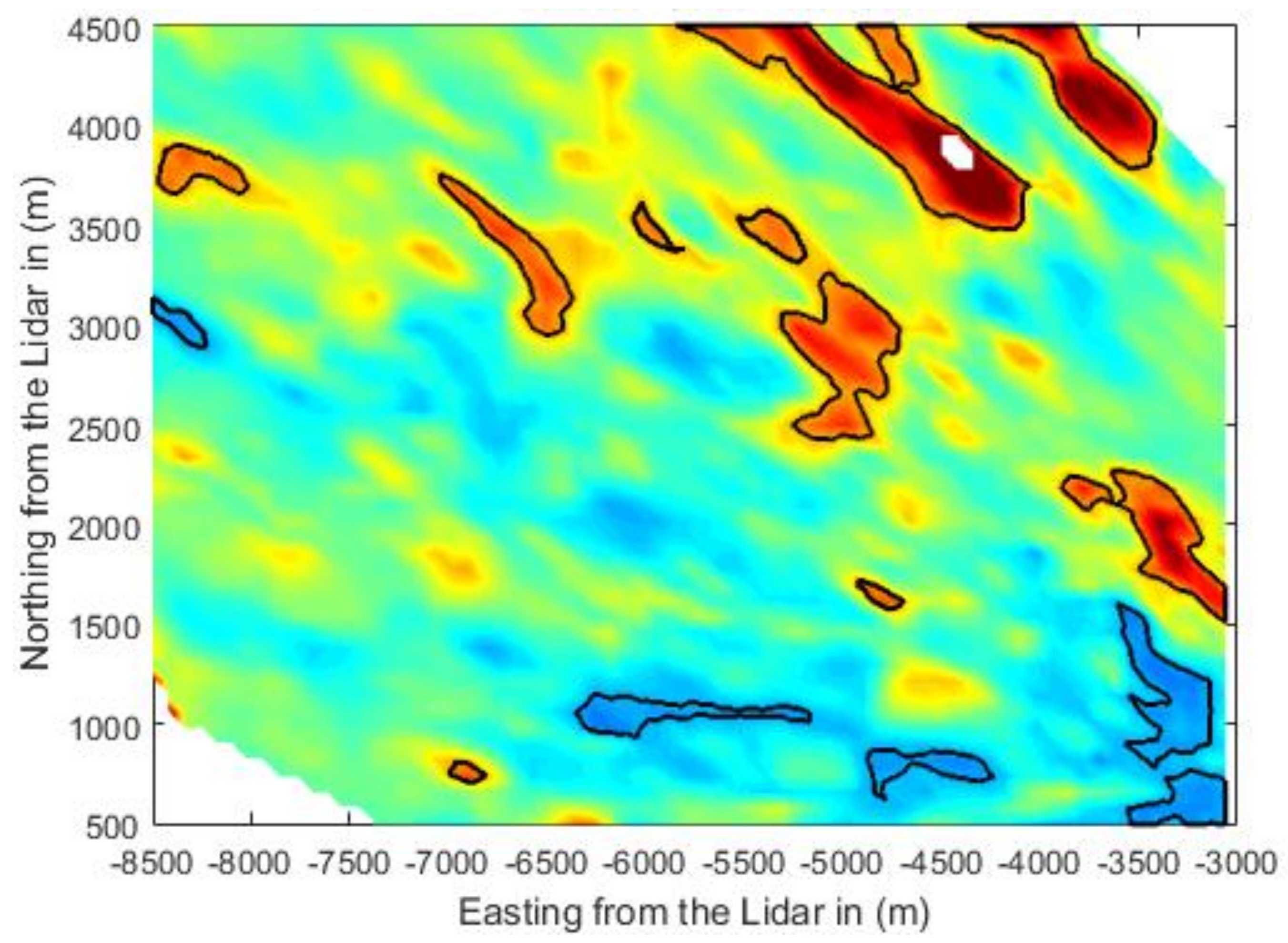
Moreover, since the patches with holes inside due to the above filtering still need to be considered as a whole, only exterior boundaries of the patches were traced. Additionally, patches with scale out of the range from 1D to 10D were filtered out and the centroids of the patches were calculated during the tracing process. The scale of a patch is defined as the square root of its area calculated by multiplying the grid area (10 m 10 m) by the number of the grid points inside or on the boundary. The retrieved wind field along with detected gust boundaries is shown in Figure 4.
2.5. Tracking of Gust Patches
To predict the future location of the gust patches, their advective characteristics need to be confirmed at first. Therefore, the next question is how to associate the patches between time frames given the detected regions. Given the formation of the spatial gust is contributed by the atmospheric turbulence, we assume that the gust regions propagate along the mean wind direction and their turbulent properties remain unchanged according to Taylor’s frozen turbulence hypothesis. Nevertheless, since the time intervals between two wind fields are integers, multiples of 30 s, they are relatively long compared to the eddies in the atmosphere, so Taylor’s hypothesis is relaxed to some extent. It means slight changes in wind speed and wind direction, variations of scales, and deformation of the shapes are allowed in the proposed algorithm.
After extracting the gust regions from the wind field at two time frames, the tracking algorithm takes the detected gusts as inputs. The patches at an earlier frame are called “original patches,” and patches at later frame are called “candidate patches.” The time interval between the two frames should not be larger than 90 s. Otherwise, the tracking algorithm will fail due to large changes in wind speed or shape caused by the evolution of the wind field.
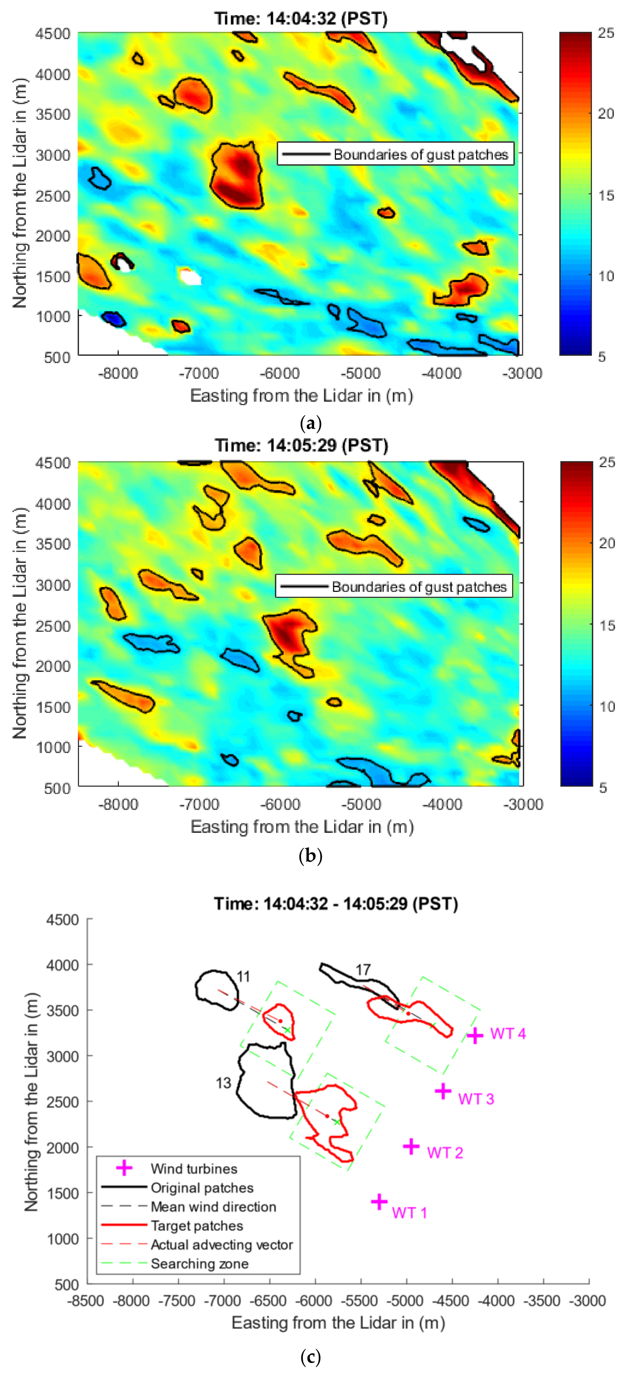
Next, a searching zone is assigned to each original patch. In the searching zone, the algorithm searches for the corresponding target patch on the second frame over all the candidate patches. The candidate patches close to the boundaries of the studied wind field are neglected because of partial observation of the patches. The searching zone is placed downstream of the original patches and oriented along the mean wind direction of the measurement domain. The distance between the original patch and the center of the searching zone is set to the product of the mean wind speed of the measurement domain and the time interval between the frames. The size of the searching zone changes adaptively because a patch could deviate further from the streamline as time elapses. In that case, a large searching zone is needed to cover the possible area that the target patch could reach. The spanwise searching range is set proportional to the product of time and the standard deviation of wind velocity in the spanwise direction, and the same method is applied in the streamwise direction. The spanwise and streamwise velocity components can be calculated by projecting the retrieved x and y velocity components to the streamwise and spanwise directions. The searching zone constrains the tracking algorithm to a small window instead of the whole domain, which avoids unnecessary calculation. Examples of the original-target patch pairs along with their searching zones are presented in Figure 5c. The wind fields are shown in Figure 5 a,b.
For an original patch, the algorithm searches for the target patch over all the candidate patches. Then, it loops the same procedure over all the other original patches. The target patch of each original patch is chosen from the candidate patches according to predefined criteria, and scores are assigned to the candidate patches for each criterion. The criteria include the changes of wind speed, the directional difference between the mean wind direction and the real moving direction, size difference, and shape deformation. For the changes of wind speed and direction, the root-mean-square deviations (RMSD) of the wind speed and direction between the points in the original and candidate patch are calculated using Equation (1), and the scores are assigned according to the RMSDs in Equation (2).
Here, the subscript “p” represents the calculated variable name, wind speed or wind direction, and stands for the value of the corresponding variable of the point i inside or on the original or candidate patch. In the calculation, we assume that the original and candidate patches share the same centroid. N represents the number of the points that are in both original and candidate patches. If a point is only in either the original or candidate patch, the point is ignored during the calculation.
For size changes and shape deformation, the intersection of union (IoU) value for each original-candidate pair is obtained by calculating the ratio of the number of intersection points to the number of union points. Here, we assume the original and candidate patch share the same centroid as well. The score for the shape change is calculated by Equation (3).
The threshold value (0.5) in Equations (2) and (3) is determined empirically. After the individual score for each criterion is obtained, the total score for each candidate patch m, , is calculated by summarizing over all the individual scores.
Patches with small difference earn high total scores, and patches with zero total scores are rejected. If multiple candidates have non-zero total scores, the one with the highest total score is chosen as the target. If such a target is identified, we claim that the original patch is advecting, and the target patch is the counterpart of the original at the second frame. Conversely, if no target is detected, the original patch loses its temporal coherency during traveling.
The tracking algorithm was tested on the wind fields shown in Figure 5a,b. Three examples of tracked original-target pairs are shown in Figure 5c. The time interval between the original and target patches is 60 s. The other patch pairs are not shown. In Figure 5, we can see many small-scale patches shown in Figure 5a are not shown inside the corresponding searching zones in Figure 5b where they should arrive after 60 s by following Taylors’ hypothesis. It provides the evidence that smaller patches are more difficult to track than larger ones. The reason would be that larger-scale patches have strong connectivity inside their internal structures, while the spatial correlation of small patches is weak and unstable. The coherency can be easily destroyed by the stretching and compression of larger-scale turbulent eddies. The destructive effect can reduce the velocity of the patches to a value beyond the threshold, deform or separate the patches, or merge small patches with other structures. All these situations can make the detecting and tracking algorithm ineffective.
2.6. Prediction of Impact
After identifying advecting patches, the arrival time and probability of arrival locations of the patches can be predicted.
2.6.1. Prediction of Impact Time
The impact time of gust patches at a certain location can be predicted using Taylor’s hypothesis, that is, dividing the distance between the gust and the location by the mean velocity. The equation is shown in Equation (5):
Both the distance and velocity are the values projected on the mean wind direction. The digression of wind speed along the streamline during traveling to the location of interest is ignored due to the negligible difference for high wind speed (>15 m/s) [6]. Equation (5) provides us with fair estimation of the arrival time, since the gust generally follows Taylor’s hypothesis in a short time period without much deviation, and this simple estimation makes the real-time prediction possible. However, spatial gusts do not always travel with the same velocity in reality. Alternatively, one can track the same patch for several time steps, calculate the actual traveling speed, and replace the mean wind speed with the obtained wind speed. Using the actual speed could improve the accuracy of the prediction, but it might also increase the complexity of the algorithm. Since the present work is to provide a fast prediction within a few seconds for wind turbine control, we focus on using the mean wind speed to calculate the arrival time.
2.6.2. Prediction of the Probability of Impact Location
If Taylor’s hypothesis holds, the gust region should arrive at a point downstream from the original patch, called the “predicted point.” However, due to the turbulent nature of the atmosphere, the real arrival point can only be estimated by a statistical probability centered at the predicted point. Here, we treat the gust patches as massless passive particles that are released from a point source, and use the concentration distribution model of plumes to model the spanwise distribution of gust patches dispersing in a turbulent wind field.
Several plume models and puff models have been developed by researchers to investigate the particle distribution in the air, such as Gaussian plume model [15,16], K-model, statistical model, and similarity model [17] etc., and more advanced but computationally more expensive models like SCIPUFF [18], RIMPUFF [19], and LODI [20]. Since this work is aimed at estimating the impact of gusts in a few seconds or minutes in advance of wind turbine control, the fast Gaussian plume model is used.
The reason for using the Gaussian plume model for wind gust studies is explained in the following. First, since the gusts travel in a relatively short distance in this study, we assume the interaction between the large-scale structures and the background turbulence is small. Therefore, we can treat the gusts as passive quantities. Second, we assume the eddy viscosity and eddy diffusivity are of comparable value, i.e., the Prandtl number is close to 1. The reason is that, according to the Reynold analysis, under stable or neutral boundary conditions, the turbulent transport of scalar quantities is similar to the transport of momentum, given the transport agents are the same [21]. In our case, the mean wind speed during the studied time period is relatively high (around 15 m/s), so the neutral boundary condition dominated the studied time period (The strong mechanical mixing due to the high wind speed balanced the buoyance-driven turbulence in the atmosphere.). Therefore, we can apply the plume model that was used for passive particles to the transportation of gust structures studied in the present work.
The original Gaussian model (Equation (6)) is modified to suit the current case: vertical distribution is neglected since only the deviation of gusts in the horizontal plane is of interest. The velocity term is removed as the probabilities will be normalized by the maximum value, meaning only relative probabilities matter. The modified equation is shown in Equation (7).
where refers to the spanwise deviation of a gust patch from the streamline with equal to zero on the streamline, and z indicates the height above the ground. In Equation (6) h is the distance from the source to the ground. is the probability at the deviation, and is the standard deviation of . We assume the turbulence field driving the gust patches is stationary and homogeneous. Taylors’ dispersion theorem provides an expression of as a function of the releasing time for stationary turbulence [17].
where is the standard deviation of the spanwise Lagrangian velocity fluctuation in which the subscript “L” stands for Lagrangian scale, and r is the autocorrelation of the spanwise velocity fluctuation. Using the random walk theory [22], the standard deviation of the deviation y, in the Lagrangian system can be approximated by Equation (8) when
and is the Lagrangian integral time scale.
Here, we assume the gust patches are ‘released’ for sufficient time () in the atmosphere, so the gust structures only advect but not disperse (grow) during traveling. It indicates that the diffusivity is constant, i.e., . As the diffusivity is defined as , Equation (9) can be deduced from the diffusivity. On the other hand, because of the stationary and homogenous turbulence assumption, the temporal correlation of the spanwise velocity fluctuation is approximated by instantaneous spatial correlation. The standard deviation of the Lagrangian velocity fluctuation was replaced by the standard deviation of Eulerian velocity fluctuation , due to instantaneous velocities being studied in this work [23]. The spanwise velocity fluctuation and its standard deviation were obtained from the given wind field. Equation (9) is transformed to
where the Lagrangian time scale , adapted from the work of Dosio et al. [24]. The reason of the adoption is that, we did not have sufficient statistical measurements for the time scale calculation in the present work, since the time interval of our lidar measurements is relatively long (30 s) and we did not have any other supplementary device installed locally. Therefore, instead of calculating the time scale directly, we adapted the result from Dosio’s simulation of a convective boundary layer. The data used in this paper is between 3 pm and 6 pm (local time), so the atmospheric flow may be expected to contain some convective activity. Therefore, we believe the selected value could be considered as the best available approximation of the time scale during the studied period. However, we suggest to use meteorological measurements (like a met mast) if available to calculate the time scale, which would improve the estimations.
Additionally, we assume the atmospheric characteristics, with respect to the meandering of gusts, are preserved during the studied period so that the Lagrangian time scale remains constant. Furthermore, the random walk theory used above is only for particles. The effect of the scales of the gusts needs to be considered in Equation (10) since we are modeling gusts. The details will be illustrated in Section 3, and the modified random walk theory is given in Equation (11). The modified random walk theory (Equation (11)) and the Gaussian model (Equation (7)) comprise the impact prediction model for advecting gust patches with different sizes.
3. Results and Discussion
3.1. Preliminary Results
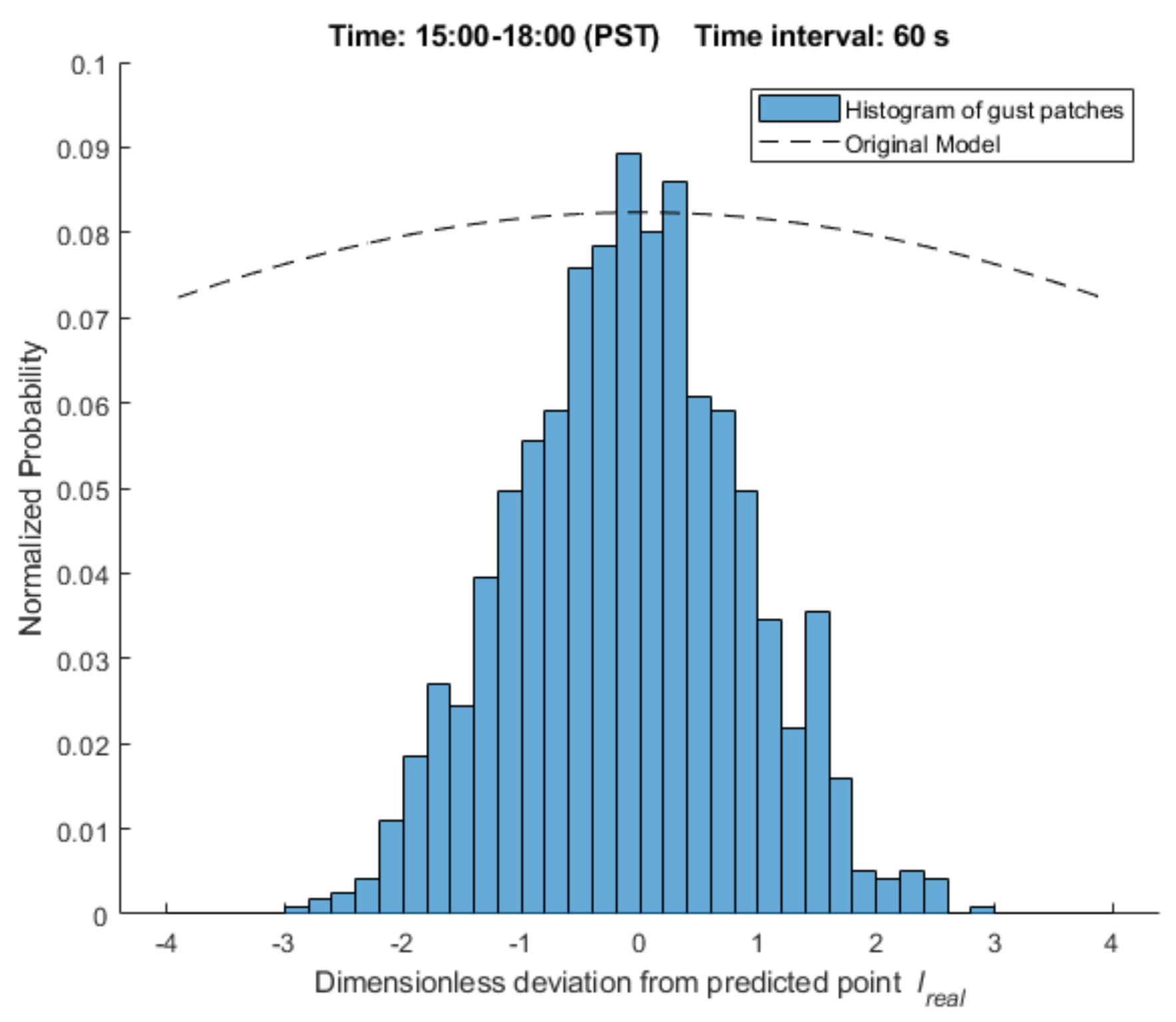
Three hours of retrieved wind fields (during 3–6 pm PST on 26 June) were processed. A time interval of 60 s between original patches and target patches was used. The original patches and corresponding target patches were extracted and associated using the detecting and tracking algorithm. Original random walk theory, Equation (10) was used for prediction. The spanwise deviation () of the target patches was measured. The spanwise deviation is defined as the deviation of the centroid of the gust from the streamline of the wind field, in the direction perpendicular to the mean wind direction of the measurement domain. Then, the spanwise deviation was normalized by the rotor diameter, i.e., , and is the dimensionless spanwise deviation. The histogram of the distribution probability of the dimensionless deviation is shown in Figure 6. The probability is normalized by the value at the ‘predicted point’. The predicted point is assumed to have the maximum probability. Figure 6 presents a Gaussian shape distribution of the gust spanwise deviation. It demonstrates our assumption that the spanwise distribution of advecting patches can be represented by a Gaussian model, rather than the exponential shape found by Branlard [6].
However, a large discrepancy was observed between the modeled distribution of the gust spanwise deviation (dashed line) and the real deviation using the detecting and tracking algorithm (histogram). The reason is that the original random walk theory does not consider the size of the particles, as the random walk theory assumes that the size difference between particles is negligible. However, the assumption does not hold for gust patches with scales in the order larger than 100 m. The size of the gusts significantly affects their movement. Small gusts are easy to move because many large-scale eddies in the atmosphere move them around, which makes their movement relatively random. On the other hand, large-scale gusts that need even larger-scale eddies to move them are more likely to flow along the streamline of the wind field. Therefore, size dependency of the gust patches needs to be considered.
3.2. Size Dependency
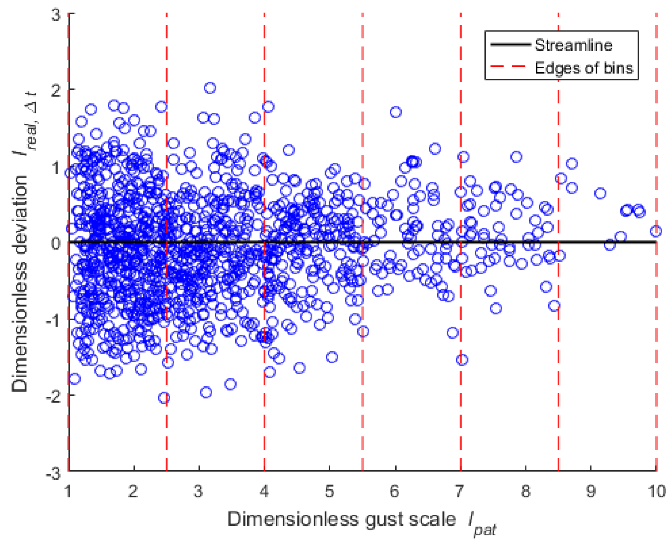
To study the effect of the size of the gusts on the spanwise deviation, the dimensionless deviation was further normalized by the square root of the time interval, i.e., , to remove the dependency of the deviation on time. The usage of the square root is according to the relationship between the deviation and time presented in Equation (10). The patch scale () was normalized by the rotor diameter, i.e., , and is the dimensionless scale. A scatter plot of the normalized deviation of all the detected patches with the dimensionless scale is shown in Figure 7. Then, the dimensionless deviations were grouped to bins according to their sizes, and inside each bin, the deviations and the dimensionless scales were averaged, respectively. The averaged values were fitted by a power function. The results and the fitting curve are plotted in Figure 8. Figure 7 and Figure 8 present a negative dependency of the deviation on the patch scale. The relationship can be well expressed by a function , where and are fitting parameters, and and is found for the current dataset.
After the size dependency was empirically derived, Equation (10) was modified to include the derived relationship by multiplying it by the derived power function.
where is the dimensionless standard deviation of the deviation y, modeled by the original random walk theory.
3.3. Improved Results Using the Modified Prediction Model
After the size dependency correction was added to Equation (10), the modified model was retested on the data presented in Figure 6. The patches were separated into three groups according to their sizes: 1D–2.5D, 2.5D–4D, and 4D–5.5D. Patches larger than 5.5D are not included due to insufficient sample points. The results are shown in Figure 9. Gaussian functions (red lines) were fitted to the histograms. The modeled distribution (black lines) were computed using Equations (7) and (11). A good match for different sizes of patches are shown in the comparison between the real measured distribution and the modeled distribution. It illustrates that the distribution probability of gust spanwise deviation can be well represented by the proposed prediction model at least for the current dataset.
3.4. Application of the Modified Prediction Model
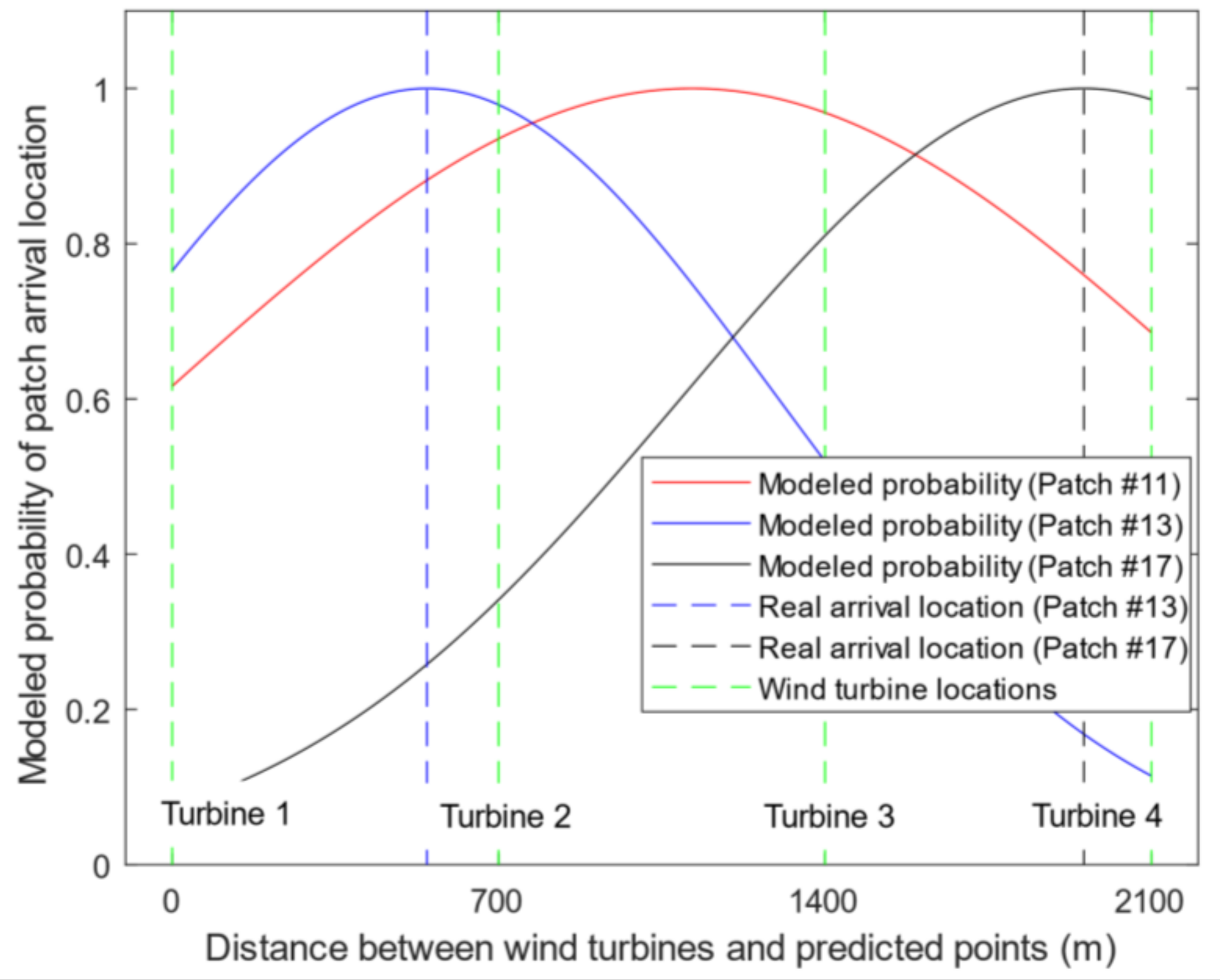
By applying the detecting and tracking algorithm to the retrieved wind field, we monitored the movement of the gusts during the three-hour period. Next, we positioned a virtual wind turbine array in the wind field shown in Figure 5a, and used the three original gusts in Figure 5c as examples, to illustrate what the time of impact and probable arrival locations of the gusts are for the hypothetical turbines. Here, the impact time and locations were calculated by the prediction model. The wind turbine array consists of four turbines that align perpendicular to the mean wind direction. The distance between two adjacent wind turbines is 700 m. The distance between the gusts and the wind turbine locations were measured, and the time taken by the gusts to reach the turbines was estimated using Equation (5). The real arrival time was also obtained by applying the detecting and tracking algorithm to the wind field at different time frames. Additionally, the spanwise distribution probabilities of the gusts at different wind turbines were predicted and are shown in Figure 10. Both predicted and real arrival time and positions are listed in Table 2. Patch 11 disappeared before reaching any wind turbine, so the real arrival time and position were left blank in Table 2 and the real arrival position is not shown in Figure 10. This fact also verifies that small patches are more difficult to track. Table 2 shows a good match between the predicted and real arrival time and locations within reasonable tolerances, which validates the proposed prediction model. However, a further quantitative validation is needed in the future work.
4. Conclusions
Due to the importance of wind gusts for wind turbine performance, spatial wind gusts with a scale from 100 m to 1000 m are studied using a Doppler lidar. A detecting and tracking algorithm for the spatial gusts is introduced. The proposed algorithm is computationally inexpensive and can provide real-time tracking and prediction. However, it is sensitive to the temporal and spatial resolution of the dataset. The algorithm was performed on a three-hour wind field data obtained from the measurements of a WindTracer Doppler lidar. The results reveal a Gaussian shape distribution of gust spanwise deviation from the streamline and a negative power-law dependency of the deviation on gust scales. Furthermore, a prediction model using the Gaussian plume model and random walk theory was introduced and corrected by the size dependency. The prediction model was tested on the same dataset, and the results further demonstrate the power law relationship. The prediction model was applied to a virtual wind turbine array to estimate the impact time and locations of the gusts on the turbines. The model was validated in a limited set of conditions, due to the lack of the dataset with a longer time period. Therefore, more quantitative validation of the model is suggested for future work. However, the major value of this work is to provide a novel approach for the study of large-scale wind gusts using a long-range Doppler lidar. In real-life applications, the proposed algorithm could be efficiently integrated to feed-forward wind turbine control systems given 2D wind fields in time series, and the wind field could be provided by a long-range Doppler lidar. Given the knowledge of the movement of potential hazardous gusts, the control system would have sufficient leading time to adjust wind turbines to optimal settings. In this case, the power generation could remain stable at the desired value, and the loads on the turbine components could be reduced. Consequently, the impact on the electric grid due to the power fluctuation could be mitigated.
Future research can be focused on the validation of the detecting and tracking algorithms on other datasets with a shorter time interval between frames and a higher spatial resolution. Using Kalman filters or other multiple object tracking algorithms, the detecting and tracking algorithm might be improved. Deep learning approaches might be expected to recognize patches quickly with acceptable accuracy. For the prediction model since the size dependency was derived empirically from the current dataset, the parameters need fine calibration for other datasets and the dependency of gusts with scales larger than 5.5D is not presently clear. In addition, the quality of the prediction model needs to be validated, which could be addressed in a dataset with longer time and in more varied atmospheric conditions. Finally, using real-time measurements, like lidar or meteorological tower, the Lagrangian time scale estimation can be improved.
Acknowledgments
We recognize the support of the Electric Power Research Institute (EPRI), sponsor award 10001389 (Program Officer: Dr. Aidan Tuohy), and a Navy Neptune Grant, Office of Naval Research (Program Officer: Dr. Rich Carlin).
Author Contributions
Kai Zhou is responsible for the study. He participated in the data collection, developed the algorithm, produced the results, and was the main writer of the manuscript. Nihanth W. Cherukuru converted the raw lidar measurements to 2D wind field. Xiaoyu Sun provided suggestions on the detecting and tracking algorithm and revisited the manuscript. Ronald Calhoun provided advisement and guidance.
Conflicts of Interest
The authors declare no conflict of interest.
References
- Schlipf, D.; Pao, L.Y.; Cheng, P.W. Comparison of feedforward and model predictive control of wind turbines using LIDAR. In Proceedings of the Conference on Decision and Control, Maui, HI, USA, 10–13 December 2012; pp. 3050–3055. [Google Scholar]
- Scholbrock, A.; Fleming, P.; Fingersh, L.; Wright, A.; Schlipf, D.; Haizmann, F.; Belen, F. Field testing LIDAR based feed-forward controls on the NREL controls advanced research turbine. In Proceedings of the 51th AIAA Aerospace Sciences Meeting Including the New Horizons Forum and Aerospace Exposition, Grapevine, TX, USA, 7–10 January 2013. [Google Scholar]
- Kumar, A.A.; Bossanyi, E.A.; Scholbrock, A.K.; Fleming, P.; Boquet, M.; Krishnamurthy, R. Field Testing of LIDAR-Assisted Feedforward Control Algorithms for Improved Speed Control and Fatigue Load Reduction on a 600-kW Wind Turbine: Preprint. Presented at the EWEA 2015 Annual Event, Golden, CO, USA, 17–20 November 2015. [Google Scholar]
- Kristalny, M.; Madjidian, D. Decentralized feedforward control of wind farms: Prospects and open problems. In Proceedings of the 2011 50th IEEE Conference on Decision and Control and European Control Conference, Orlando, FL, USA, 12–15 December 2011; pp. 3464–3469. [Google Scholar]
- International Electrotechnical Commission. International Standard, IEC 61400-1, Wind Turbines—Part 1: Design Requirements, 3rd ed.; International Electrotechnical Commission: Geneva, Switzerland, 2005. [Google Scholar]
- Branlard, E. Wind energy: On the statistics of gusts and their propagation through a wind farm. ECN-Wind-Memo-09-005Master’s Thesis, Energy research Centre of the Netherlands, Petten, The Netherlands, February 2009. [Google Scholar]
- Beljaars, A.C. The Measurement of Gustiness at Routine Wind Stations: A Review; World Meteorological Organization: Geneva, Switzerland, 1987. [Google Scholar]
- Kelley, N.; Shirazi, M.; Jager, D.; Wilde, S.; Adams, J.; Buhl, M.; Patton, E. Lamar Low-Level Jet Project Interim Report; Technical Paper No. NREL/TP-500-34593; National Renewable Energy Laboratory, National Wind Technology Center: Golden, CO, USA, 2004.
- Chamorro, L.P.; Lee, S.J.; Olsen, D.; Milliren, C.; Marr, J.; Arndt, R.E.A.; Sotiropoulos, F. Turbulence effects on a full-scale 2.5 MW horizontal-axis wind turbine under neutrally stratified conditions. Wind Energy 2015, 18, 339–349. [Google Scholar] [CrossRef]
- Mayor, S.D.; Lowe, J.P.; Mauzey, C.F. Two-component horizontal aerosol motion vectors in the atmospheric surface layer from a cross-correlation algorithm applied to scanning elastic backscatter lidar data. J. Atmos. Ocean. Technol. 2012, 29, 1585–1602. [Google Scholar] [CrossRef]
- Mayor, S.D.; Dérian, P.; Mauzey, C.F.; Hamada, M. Two-component wind fields from scanning aerosol lidar and motion estimation algorithms. In Proceedings of the SPIE Optical Engineering+ Applications, San Diego, CA, USA, 17 September 2013; p. 887208. [Google Scholar]
- Cherukuru, N.W.; Calhoun, R.; Krishnamurthy, R.; Benny, S.; Reuder, J.; Flügge, M. 2D VAR single Doppler lidar vector retrieval and its application in offshore wind energy. Energy Proced. 2017, 137, 497–504. [Google Scholar] [CrossRef]
- Amidror, I. Scattered data interpolation methods for electronic imaging systems: A survey. J. Electron. Imaging 2002, 11, 157–177. [Google Scholar] [CrossRef]
- Moore-Neighbor Tracing. Available online: http://www.imageprocessingplace.com/downloads_V3/root_downloads/tutorials/contour_tracing_Abeer_George_Ghuneim/moore.html (accessed on 9 October 2017).
- Batchelor, G.K. Diffusion in a field of homogeneous turbulence: II. The relative motion of particles. In Mathematical Proceedings of the Cambridge Philosophical Society; Cambridge University Press: Cambridge, UK, 1952; pp. 345–362. [Google Scholar]
- Petersen, W.B.; Catalano, J.A.; Chico, T.; Yuen, T.S. INPUFF-A Single Source Gaussian Puff Dispersion Algorithm: User’s Guide; US EPA: Research Triangle Park, NC, USA, 1984.
- Hanna, S.R.; Briggs, G.A.; Hosker, R.P., Jr. Handbook on Atmospheric Dispersion; Technical Information Center, U.S. Department of Energy: Washington, DC, USA, 1982.
- Sykes, R.I.; Parker, S.F.; Henn, D.S.; Cerasoli, C.P.; Santos, L.P. PC-SCIPUFF Version 1.2 PD Technical Documentation; ARAP Report No. 718; Titan Corporation, Titan Research & Technology Division, ARAP Group: Princeton, NJ, USA, 1998. [Google Scholar]
- Thykier-Nielsen, S.; Deme, S.; Mikkelsen, T. Description of the atmospheric dispersion module RIMPUFF. 1999. Available online: https://s3.amazonaws.com/academia.edu.documents/39632120/Description_of_the_atmospheric_dispersio20151103-1858-w1thfx.pdf?AWSAccessKeyId=AKIAIWOWYYGZ2Y53UL3A&Expires=1521966958&Signature=vnkIK16SU2hvkTa3L7PZWujwIB8%3D&response-content-disposition=inline%3B%20filename%3DDescription_of_the_atmospheric_dispersio.pdf (accessed on 25 March 2018).
- Leone, J.M., Jr.; Nasstrom, J.S.; Maddix, D.M.; Larson, D.J.; Sugiyama, G.; Ermak, D.L. Lagrangian Operational Dispersion Integrator (LODI) User’s Guide; Report UCRL-AM-212798; Lawrence Livermore National Laboratory: Livermore, CA, USA, 2005.
- Li, D.; Katul, G.G.; Zilitinkevich, S.S. Revisiting the turbulent Prandtl number in an idealized atmospheric surface layer. J. Atmos. Sci. 2015, 72, 2394–2410. [Google Scholar] [CrossRef]
- Kundu, P.K.; Cohen, I.M.; Dowling, D.W. Fluid Mechanics, 4th ed.; Academic Press: Burlington, MA, USA, 2008. [Google Scholar]
- Price, J.F. Lagrangian and Eulerian representations of fluid flow: Part I, kinematics and the equations of Motion; Clark Laboratory Woods Hole Oceanographic Institution: Woods Hole, MA, USA, 2005. [Google Scholar]
- Dosio, A.; Guerau de Arellano, J.V.; Holtslag, A.A.; Builtjes, P.J. Relating Eulerian and Lagrangian statistics for the turbulent dispersion in the atmospheric convective boundary layer. J. Atmos. Sci. 2005, 62, 1175–1191. [Google Scholar] [CrossRef]
Figure 1.
Wind field retrieved by the two-dimensional variational analysis method (2D-VAR) algorithm. Background colors indicate the magnitude of the local wind speed, and the arrows show the local wind direction.
Figure 1.
Wind field retrieved by the two-dimensional variational analysis method (2D-VAR) algorithm. Background colors indicate the magnitude of the local wind speed, and the arrows show the local wind direction.
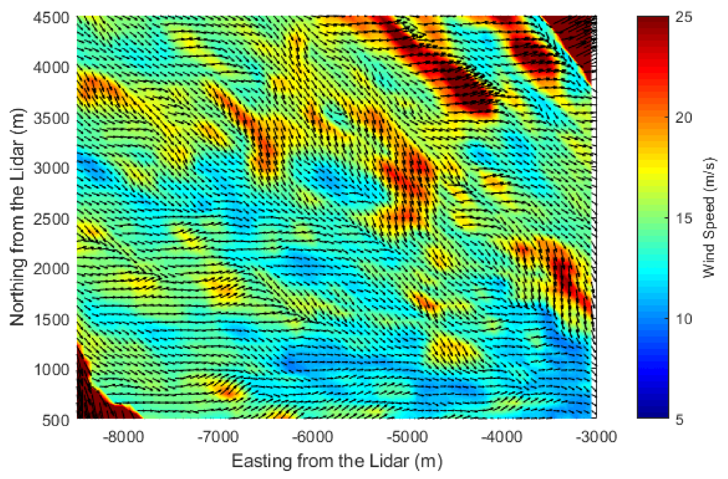
Figure 2.
Wind field in Figure 1 after data preprocessing. Colors indicate the magnitude of the local wind speed.
Figure 2.
Wind field in Figure 1 after data preprocessing. Colors indicate the magnitude of the local wind speed.
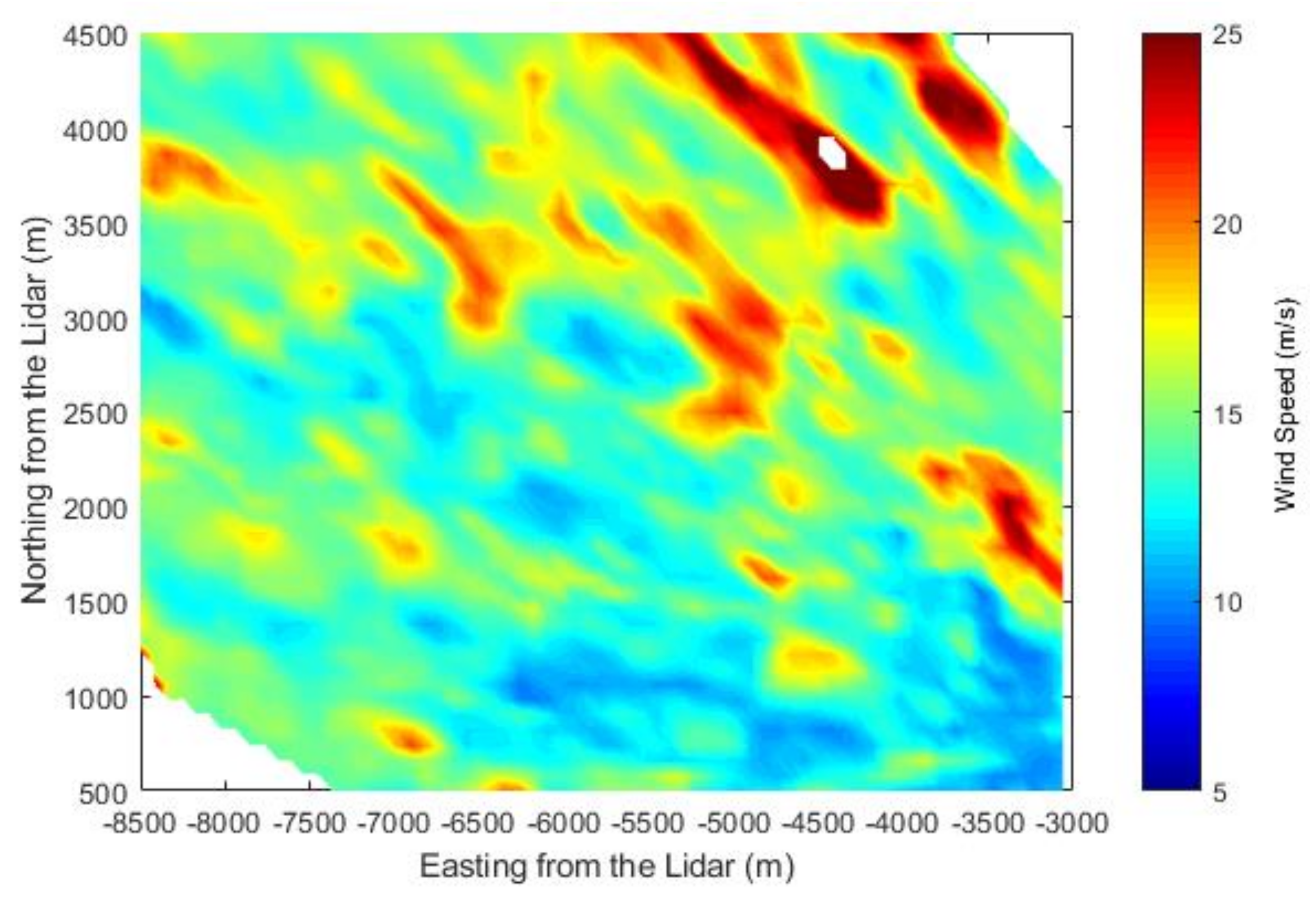
Figure 3.
Extracted gust regions in black-white scale from the wind field in Figure 2. The gust regions are in white.
Figure 3.
Extracted gust regions in black-white scale from the wind field in Figure 2. The gust regions are in white.
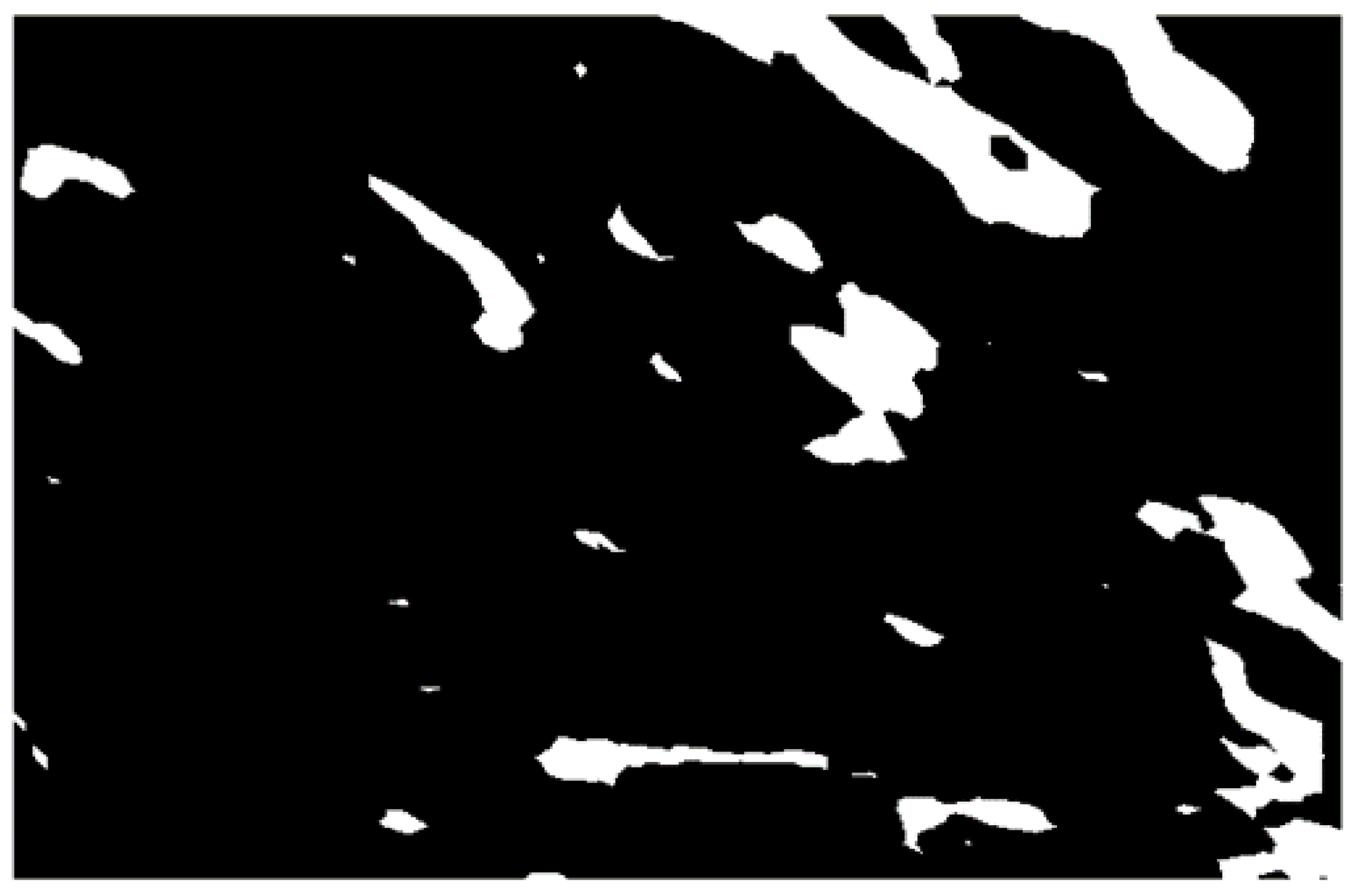
Figure 4.
Retrieved wind field with detected boundaries of gust regions. Black contours are the boundaries of the detected patches.
Figure 4.
Retrieved wind field with detected boundaries of gust regions. Black contours are the boundaries of the detected patches.

Figure 5.
(a) Wind field at the first time frame. Colors indicate the wind speed. Black contours are the boundaries of detected patches; (b) Wind field at the second time frame; (c) Example original- target patch pairs. Black patches are the original gust regions extracted from (a), and red patches are the corresponding target gust regions extracted from (b). Green dashed boxes are the searching zones. Black and red dashed lines indicate the moving direction of the streamline and the real movement of the patches, respectively. Pink crosses indicate the locations of a virtual wind turbine array.

Figure 6.
Normalized distribution probability of the spanwise deviation of patches from the predicted points. The dashed line represents the normalized probability modeled by Equation (10), and the histogram shows the normalized probability of the real spanwise deviations.
Figure 6.
Normalized distribution probability of the spanwise deviation of patches from the predicted points. The dashed line represents the normalized probability modeled by Equation (10), and the histogram shows the normalized probability of the real spanwise deviations.

Figure 7.
Scatter plot of normalized deviations and patch scales. The streamline overlays the line with the deviation equal to zero. The red dashed lines imply the edges of the bins. The average dimensionless scales at the bins are 1.75, 3.25, 4.75, 6.25, 7.75, and 9.25.
Figure 7.
Scatter plot of normalized deviations and patch scales. The streamline overlays the line with the deviation equal to zero. The red dashed lines imply the edges of the bins. The average dimensionless scales at the bins are 1.75, 3.25, 4.75, 6.25, 7.75, and 9.25.

Figure 8.
The relationship between dimensionless deviations and dimensionless gust scales. Circles are the average dimensionless deviations at different average gust scales, and the solid line is the fitting curve.
Figure 8.
The relationship between dimensionless deviations and dimensionless gust scales. Circles are the average dimensionless deviations at different average gust scales, and the solid line is the fitting curve.
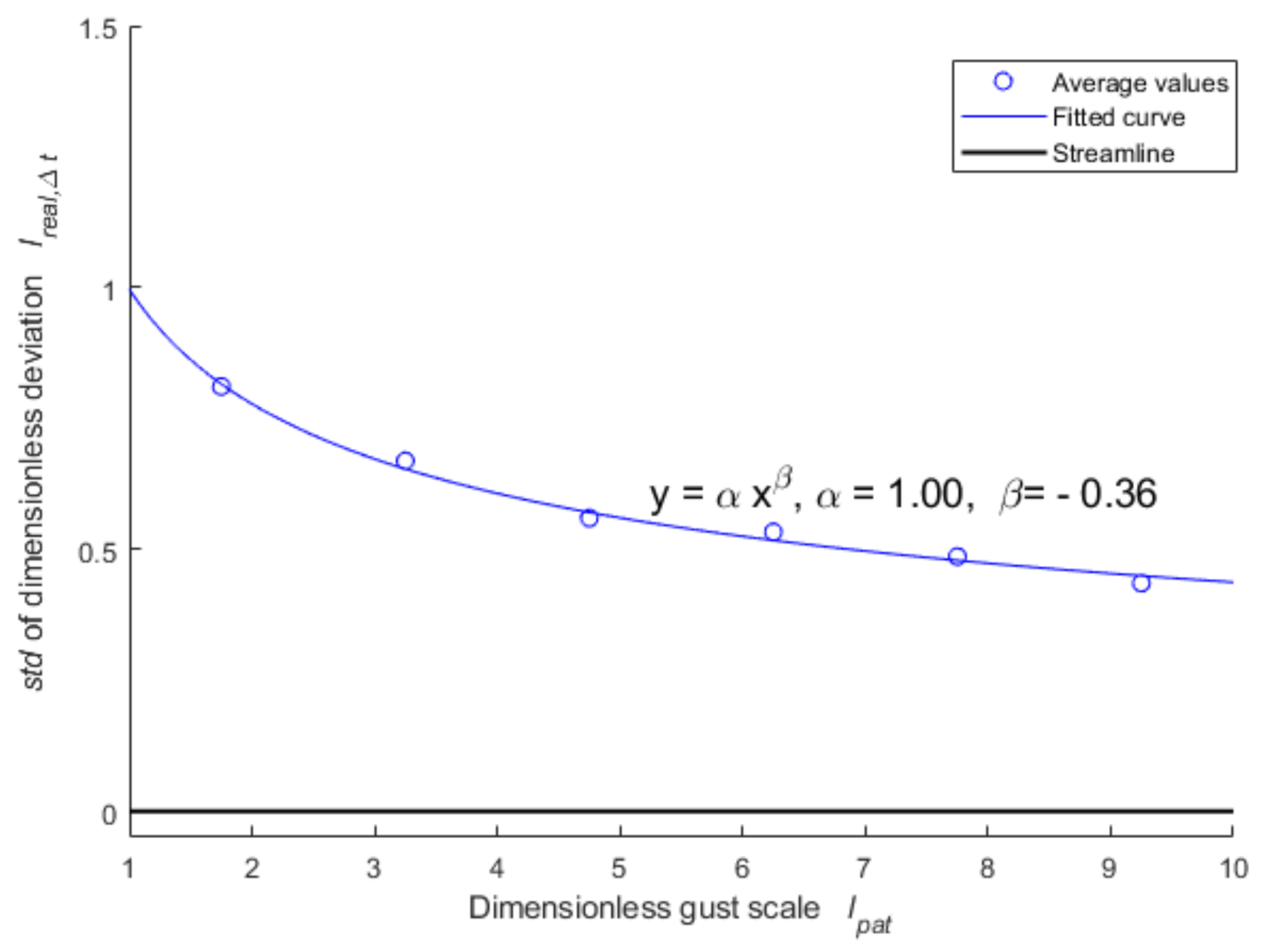
Figure 9.
Normalized distribution probability of the modeled deviation (black lines) and real deviation (histogram) of the patches. The red lines are the fitting curves to the histograms. The same dataset was used as in Figure 6. The patches were separated into three groups according to their sizes.
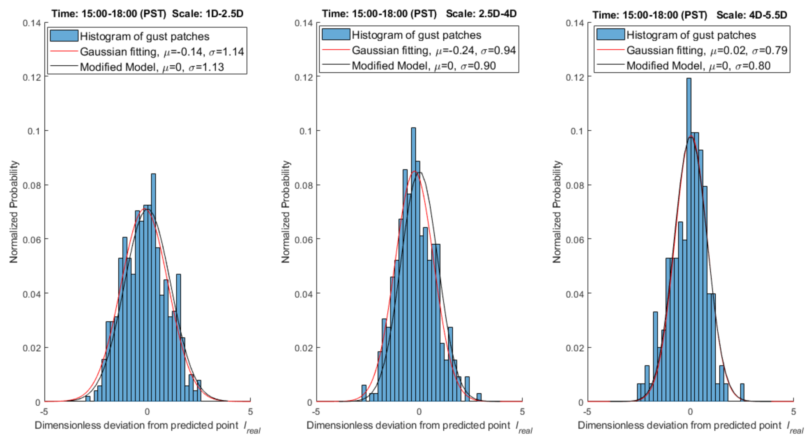
Figure 10.
Real and predicted arrival positions, and predicted normalized spanwise distribution probability of the gusts. The patch numbers correspond to the gust numbers in Figure 5c. Green dash lines indicate the locations of the wind turbines relative to Turbine 1, and the distance is measured along the wind turbine array. The blue and black dash lines represent the real arrival positions of Patch 13 and 17, respectively. Since Patch 11 disappeared before arriving any wind turbine, no line indicates its real arrival location in the figure.

Table 1.
Specifications of the Doppler lidar.
| Parameters | Settings |
|---|---|
| Wavelength | 1.6 m |
| Pulse energy | 2 mJ |
| Pulse repetition frequency | 750 Hz |
| Range resolution | 100 m |
| Blind zone | 436 m |
| Max range | 10 km |
Table 2.
Predicted and real arrival time and position of patches.
| Patch Number | #11 | #13 | #17 |
|---|---|---|---|
| Impact wind turbine | Turbine 3 | Turbine 2 | Turbine 4 |
| Predicted arrival time | 183.03 s | 116.37 s | 92.9 s |
| Real arrival time | - | ~119.54 s | ~119.54 s |
| Spanwise distance between predicted arrival position and wind turbine of impact | 285.2 m (to its left) | 153.7 m (to its left) | 144.9 m (to its left) |
| Spanwise distance between real arrival position and wind turbine of impact | - | 106.16 m (to its left) | 87.48 m (to its left) |
© 2018 by the authors. Licensee MDPI, Basel, Switzerland. This article is an open access article distributed under the terms and conditions of the Creative Commons Attribution (CC BY) license (http://creativecommons.org/licenses/by/4.0/).
Share and Cite
MDPI and ACS Style
Zhou, K.; Cherukuru, N.; Sun, X.; Calhoun, R. Wind Gust Detection and Impact Prediction for Wind Turbines. Remote Sens. 2018, 10, 514. https://doi.org/10.3390/rs10040514
AMA Style
Zhou K, Cherukuru N, Sun X, Calhoun R. Wind Gust Detection and Impact Prediction for Wind Turbines. Remote Sensing. 2018; 10(4):514. https://doi.org/10.3390/rs10040514
Chicago/Turabian StyleZhou, Kai, Nihanth Cherukuru, Xiaoyu Sun, and Ronald Calhoun. 2018. "Wind Gust Detection and Impact Prediction for Wind Turbines" Remote Sensing 10, no. 4: 514. https://doi.org/10.3390/rs10040514
Note that from the first issue of 2016, this journal uses article numbers instead of page numbers. See further details here.