A Deep Pipelined Implementation of Hyperspectral Target Detection Algorithm on FPGA Using HLS

 , , ,
, , ,  ,
,
Abstract
:
1. Introduction
- A novel deep pipelined architecture is proposed to accelerate the proposed DPBS-CEM algorithm on FPGA using HLS. It outperforms the previous work designed with RTL in terms of data throughput performance.
- A solution is derived to remove the data dependency existing in SBS-CEM for updating the inverse matrices, by allowing four adjacent pixels to update their own individual inverse matrices that are stored in four different memories.
- The proposed structure can be simply rebuilt to support diverse HSI implementations with different spatial resolution and number of spectral bands through several parameters modified under HLS. Most importantly, the framework can support various operation modes including split/non-split data and local/global detection. It is easily adapted to match multiple rates of hyperspectral imagery.
- Last but not least, alternative solutions to the problems of feedback and high fanout are also provided.
2. Related Algorithms
2.1. CEM Algorithm
2.1.1. Principle of the CEM Algorithm
2.1.2. Problem Analysis
2.2. SBS-CEM Algorithm
2.2.1. Principle of the SBS-CEM Algorithm
2.2.2. Problem Analysis
3. Algorithm Optimization
3.1. Principle of Algorithm Optimization
| Algorithm 1 The deep pipelined background statistics (DPBS) target detection CEM algorithm |
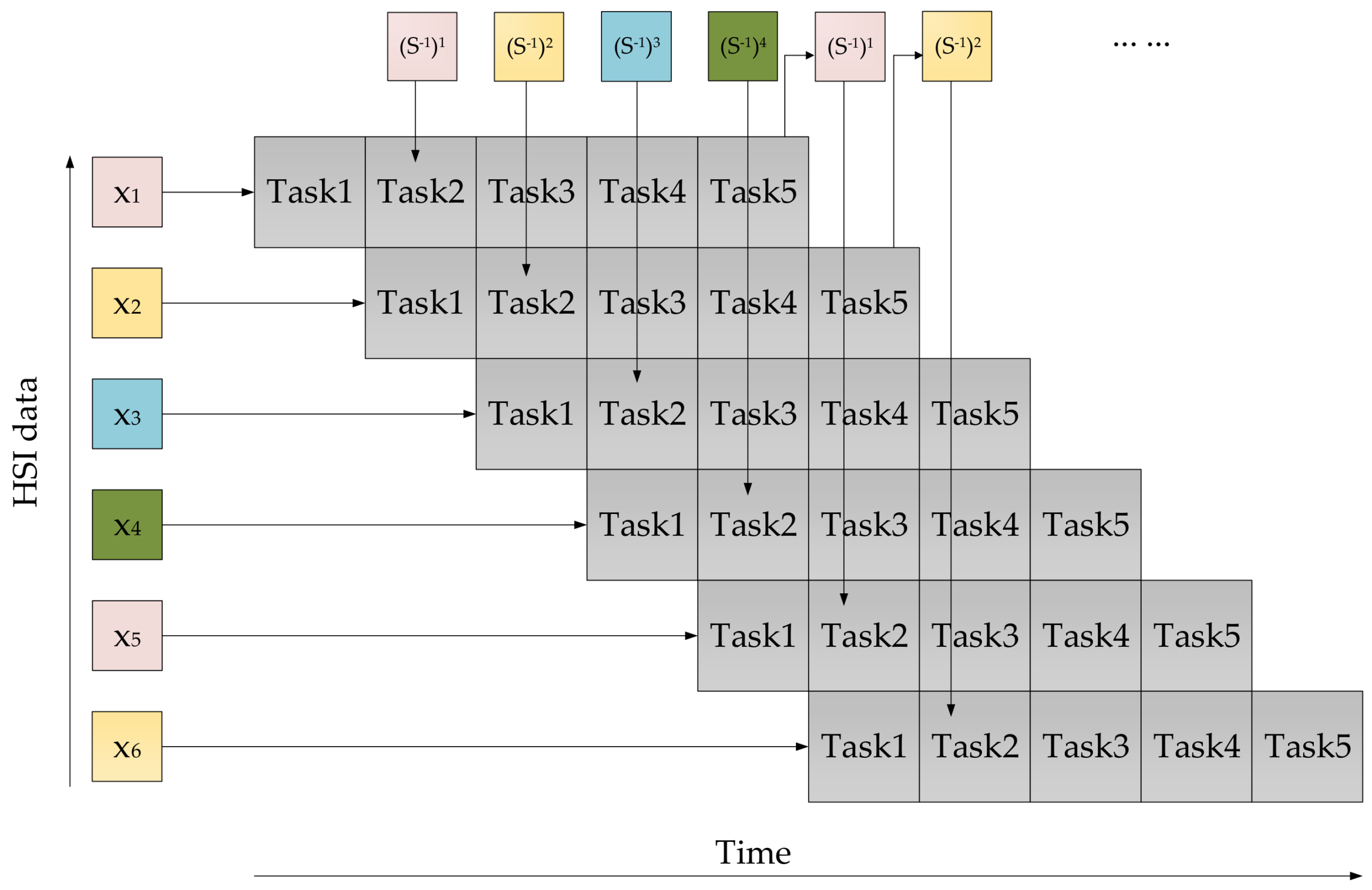
Input: Initialize the following parameters. (1) HSI data size: ; (2) the value of ; (3) the desired signature ; (4) the number of inverse matrices: ; (5) indicates the index of number; (6) K indicates the number of pixel vectors collected before starting target detection; Output: the final target detection results. define an initial inverse matrix : data segmentation: ; ; calculate the inverse matrix: calculate the target detection results: |
3.2. Design Challenges
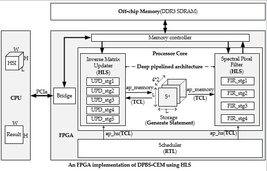
4. FPGA Implementation
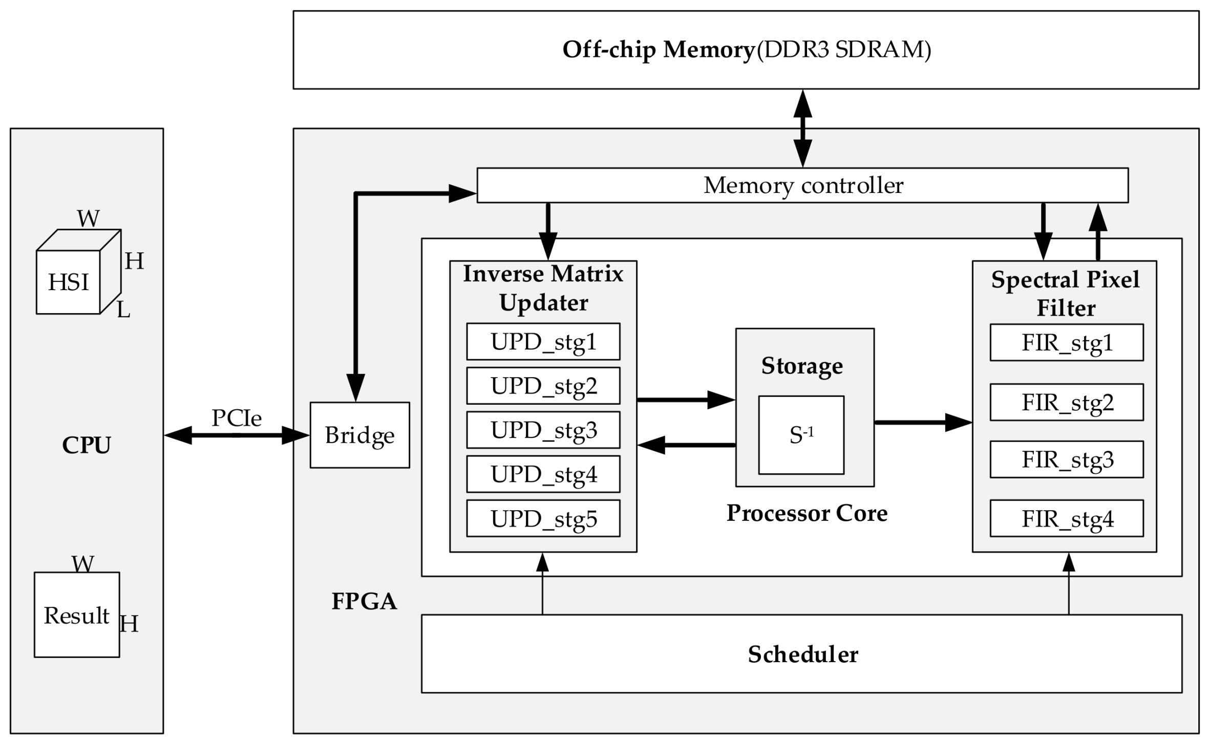
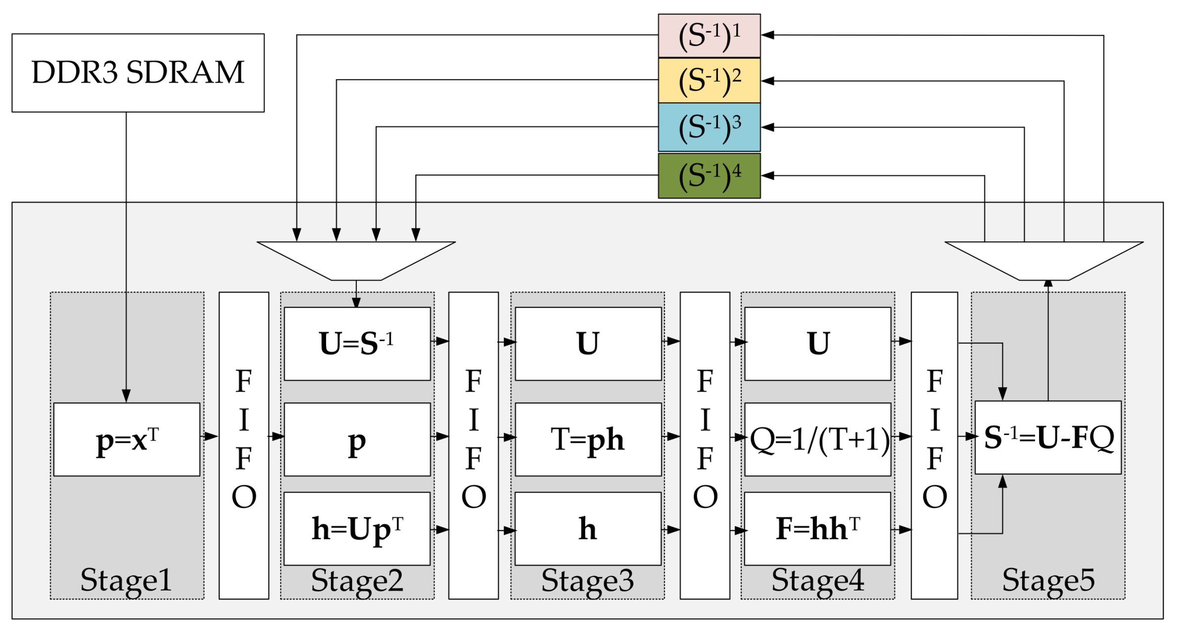
4.1. Overall Hardware Architecture of DPBS-CEM
4.2. Update Process of Inverse Matrix
4.2.1. Internal Architecture
- Stage1
- All elements of vector read from the DDR3 SDRAM are loaded sequentially and passed on to the next stage.
- Stage2
- According to the index of the current pixel, we read a corresponding matrix from the storage module. When dealing with the first four pixels of an image, we need to overwrite the matrix with initialized matrix . Then, we take matrix and vector as input operands into the Block A to calculate product . Subsequently, , , and are passed to the next stage.
- Stage3
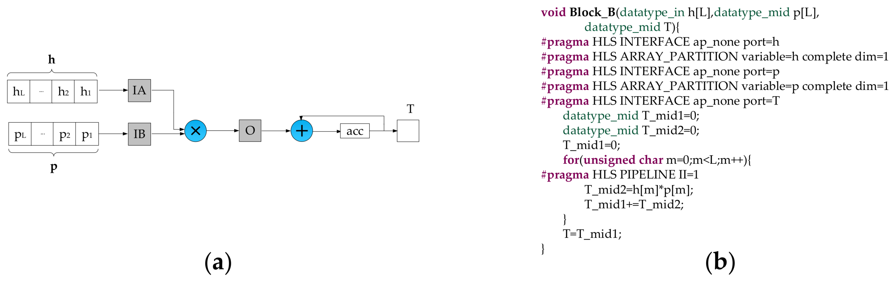
- We count T by applying the Block B, then transmit , T, and to the next stage.
- Stage4
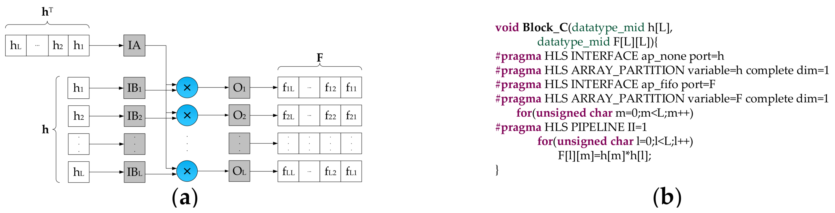
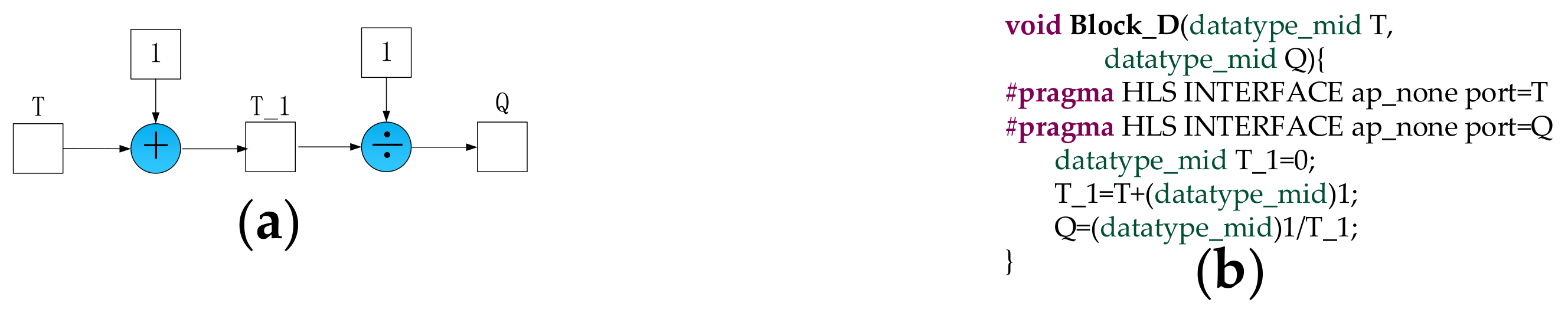
- The Block C is utilized to work out the product of two vectors. We calculate Q by employing the Block D. Then , , and Q are delivered to the next stage.
- Stage5
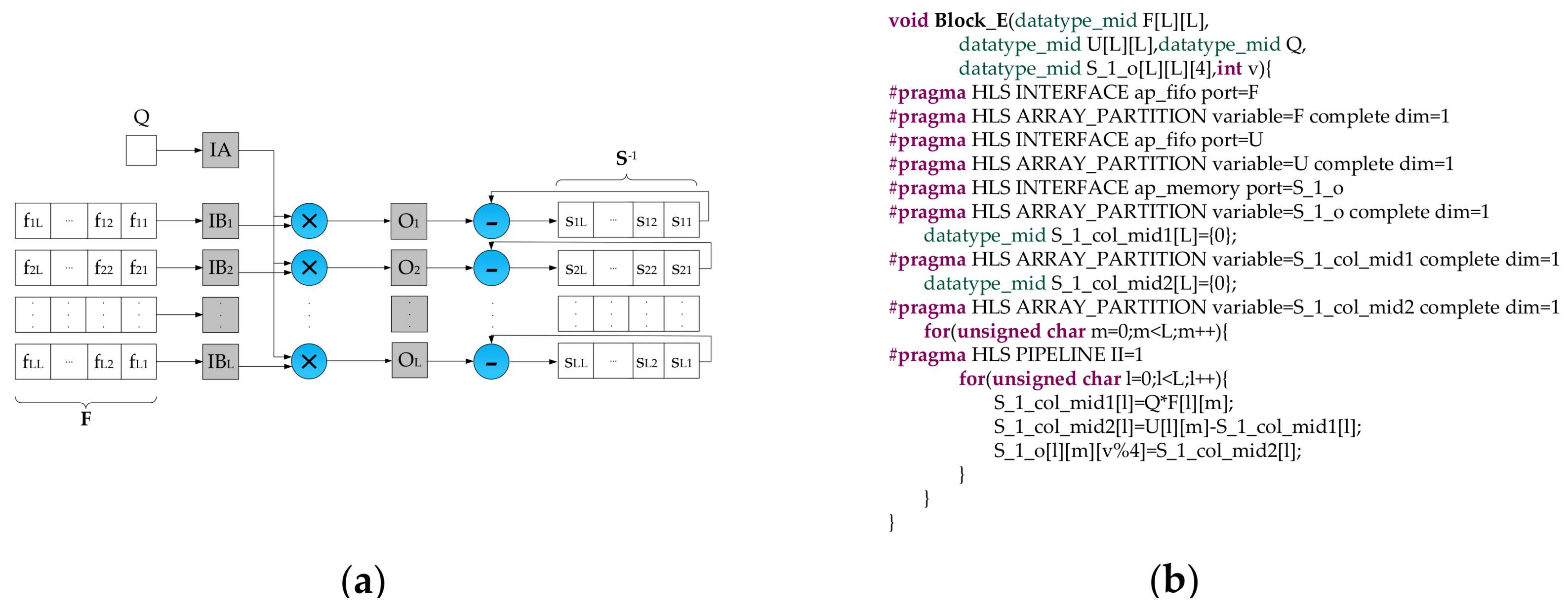
- We figure out the new matrix through utilizing the Block E and write it to the corresponding location of the storage module according to the current pixel.
- (1)
- In the process of updating the inverse matrices, we allocate a single divider and execute it once for each inverse matrix updating. Thanks to such operation, a lot of logic resources and computation time consumed by the divider can be saved.
- (2)
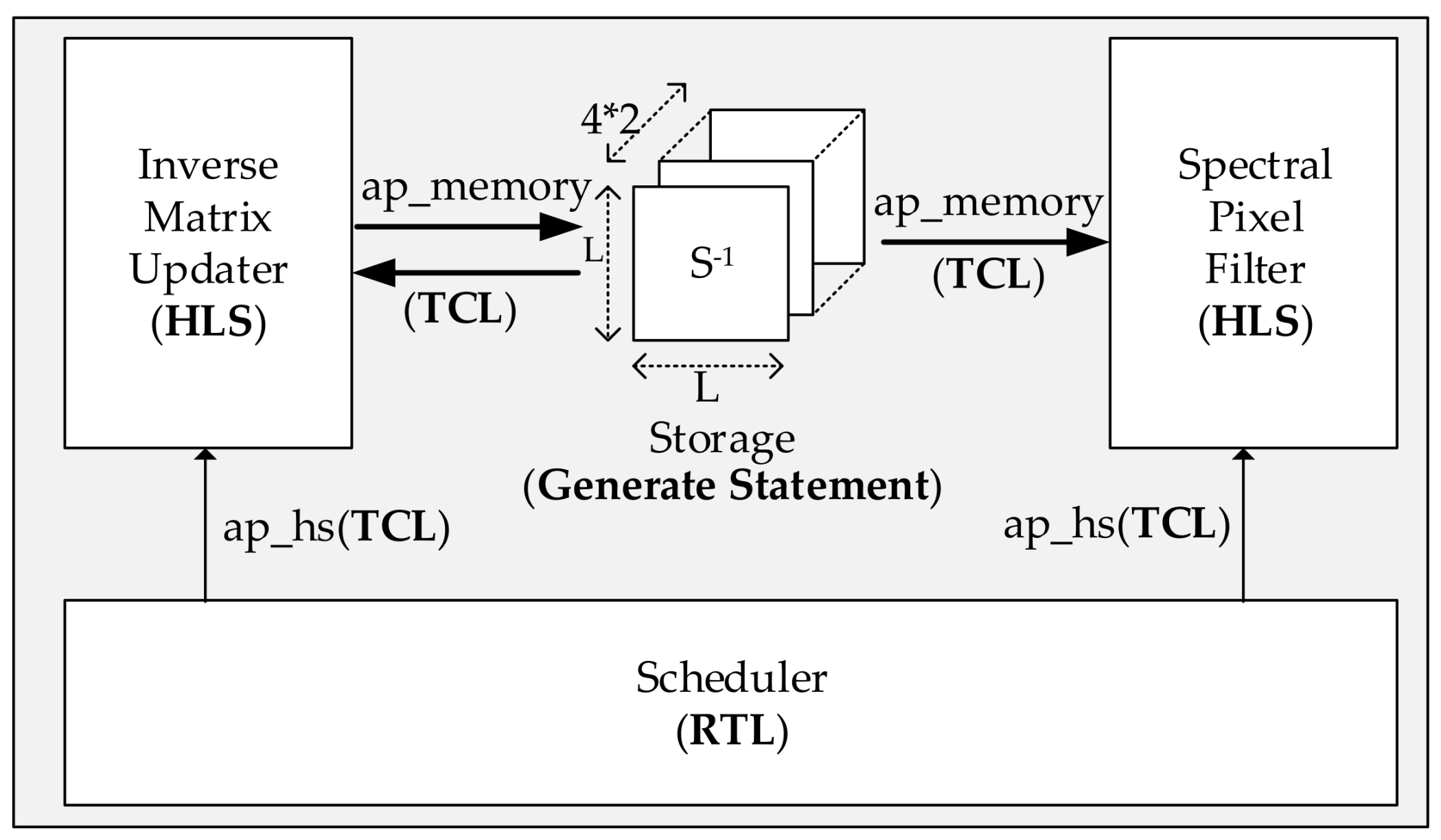
- There are three types of data that need to be cached between two stages, the scalar data, the vector data, and the matrix data. In order to attain the capability of parallel computation, the matrix is cached in L first in first out (FIFO) memories (In HLS, we use the STREAM directive to map these sorts of data into FIFOs). While the elements of a vector are realized as registers. In addition, L simple dual port RAMs (simple DPRAMs) are deployed to implement the storage module.
- (3)
- The data type of input data is 16 bits signed fixed-point (15 bits fractional part), while the data type of intermediate data and detection results are not easy to assign. Due to the precision of intermediate data and detection results have a significant impact not only on the detection accuracy but also on the resource consumption, we performed some experiments to explore the relationship between the data precision and the detection accuracy. The experimental results demonstrate that the detection accuracy goes up with the increase of the bit-width of the fractional part. To better balance the trade-off between the detection accuracy and the resource consumption, we use different data types in different stages. As shown in Figure 2, the variable T and Q are defined as 38 bits signed fixed-point type (14 bits integer part, 23 bits fractional part). The elements of the matrix F are 32 bits signed fixed-point type (14 bits integer part, 17 bits fractional part). All the other intermediate data are represented as 32 bits signed fixed-point type (7 bits integer part, 24 bits fractional part). T and Q have the significant impact on the detection accuracy. Therefore, they are assigned high data precision up to 38 bits. The elements of the matrix F are obtained by the accumulation operations, and more bits should be assigned to the integer part for avoiding data overflow. Though T and Q have larger bit-width up to 38 bits, it almost does not increase the logic resource consumption compared with the data type of 32 bits signed fixed-point. The reason is that only one single accumulation adder is allocated to compute T while one single adder and one single divider are placed to calculate Q. It is worthwhile to highlight that these data types can be defined and modified by HLS ap_fixed type easily.
4.2.2. Deep Pipeline
- (1)
- For the purpose of reducing logic resources without compromising accuracy, we implement a high-precision division with the price of long latency. It takes near 30 clock cycles to output the division result. If the division operation is assigned to Task3, the running time of Task3 will increase a lot. As a result, Task3 will turn out to be a bottleneck in the pipeline. Therefore, we assign the division operation to Task4. Note that, the division and multiplication operations in Task4 are carried out simultaneously.
- (2)
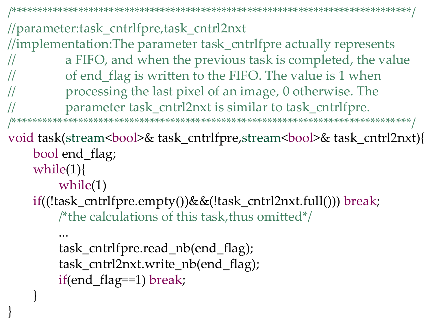
- For each task, it does not start until all input data are ready and all output FIFOs are not full. It can be simply realized in HLS by writing C/C++ code as shown in Figure 9. To make the pipeline run efficiently, these FIFOs, which are dedicated to bridging two adjacent tasks, are designed a little bit larger. In this work, the depth of FIFO for vector is 2, while the depth of FIFO for the matrix is . Besides, the depth of simple DPRAM for the storage module is .
- (3)
- With regard to the execution time of each task, it is consistent with times of the system clock period. Among them, the input time of an L-dimensional vector is L clock cycles, the delay time of the multiplier is one clock cycle, and the remaining 11 clock cycles are used to control input/output of the task. Especially, because two extra clock cycles are required for overwriting the matrix with the initialized matrix , the total execution time of Task2 is clock cycles.
4.3. Difficulties with Using HLS
4.3.1. Feedback
4.3.2. High Fanout
4.4. Specific Features
4.4.1. Scalability and Portability
4.4.2. Flexibility
5. Experimental Results and Analysis
5.1. Hyperspectral Image Data Set
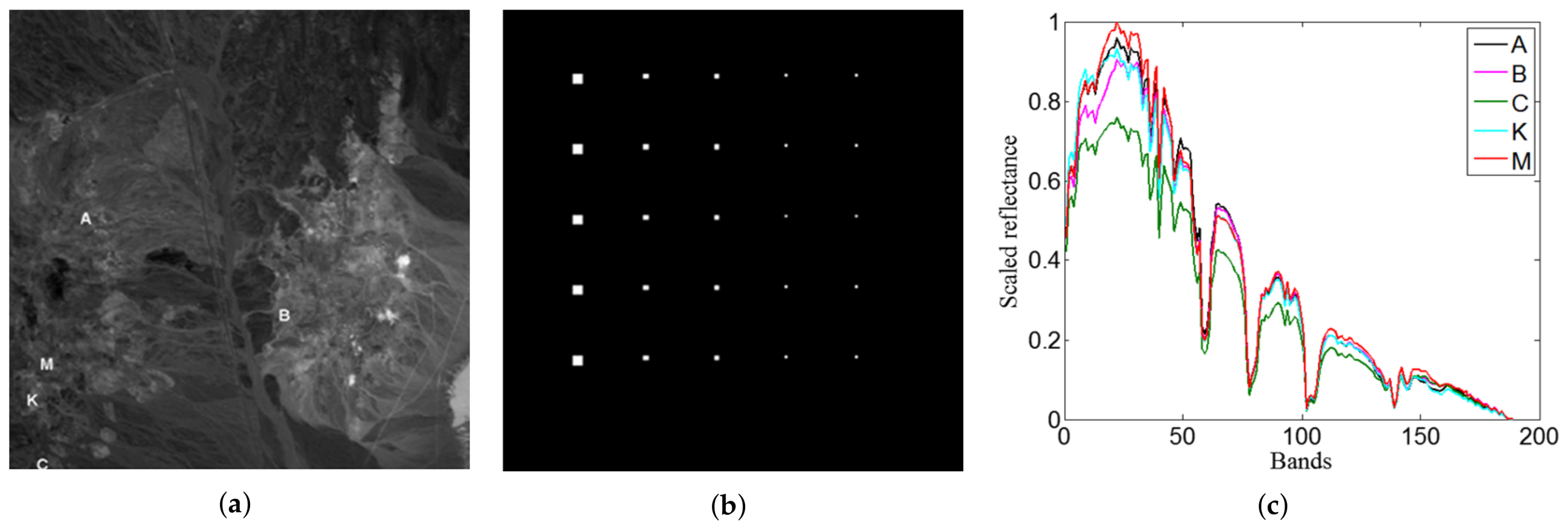
5.1.1. TE1 Image
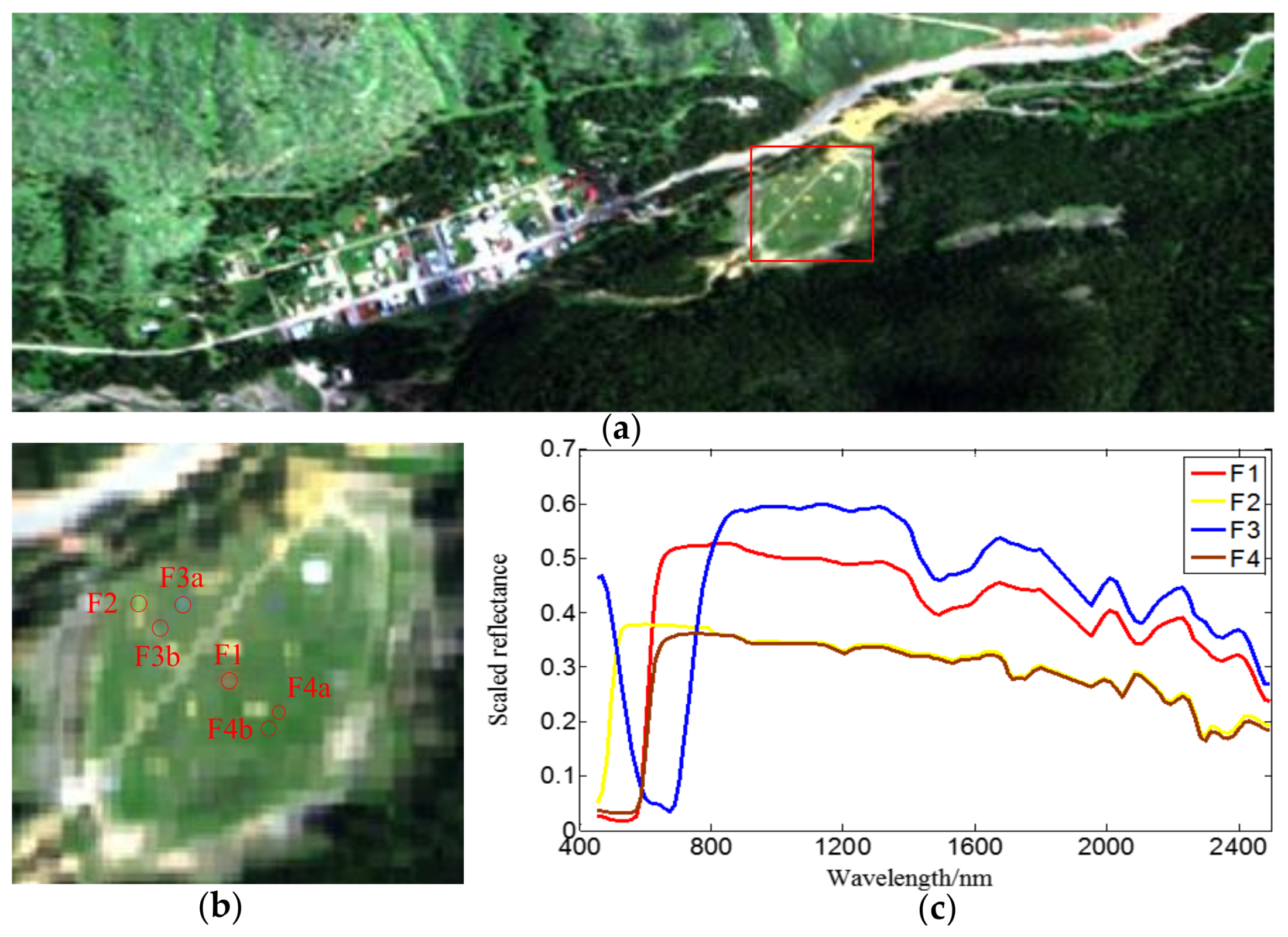
5.1.2. HyMap Reflectance Image
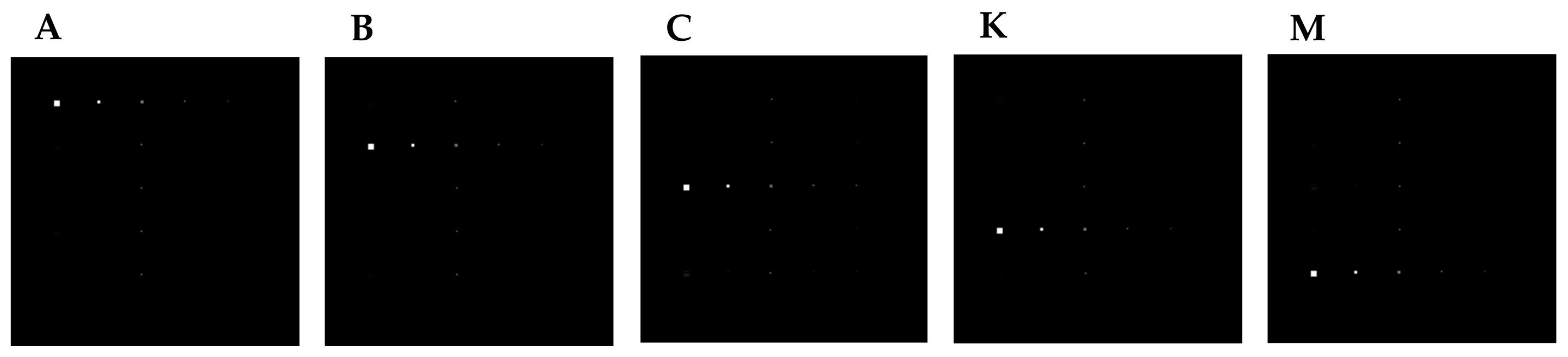
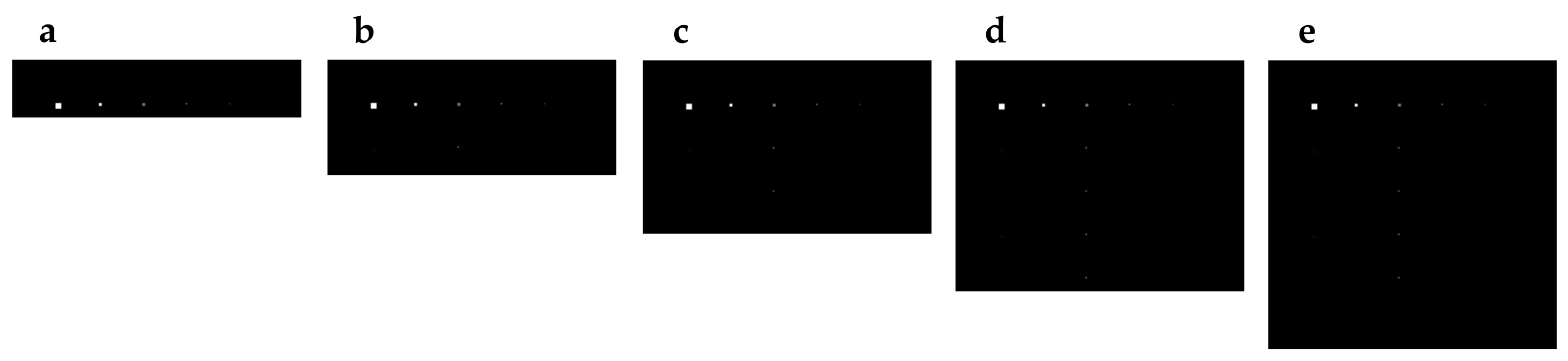
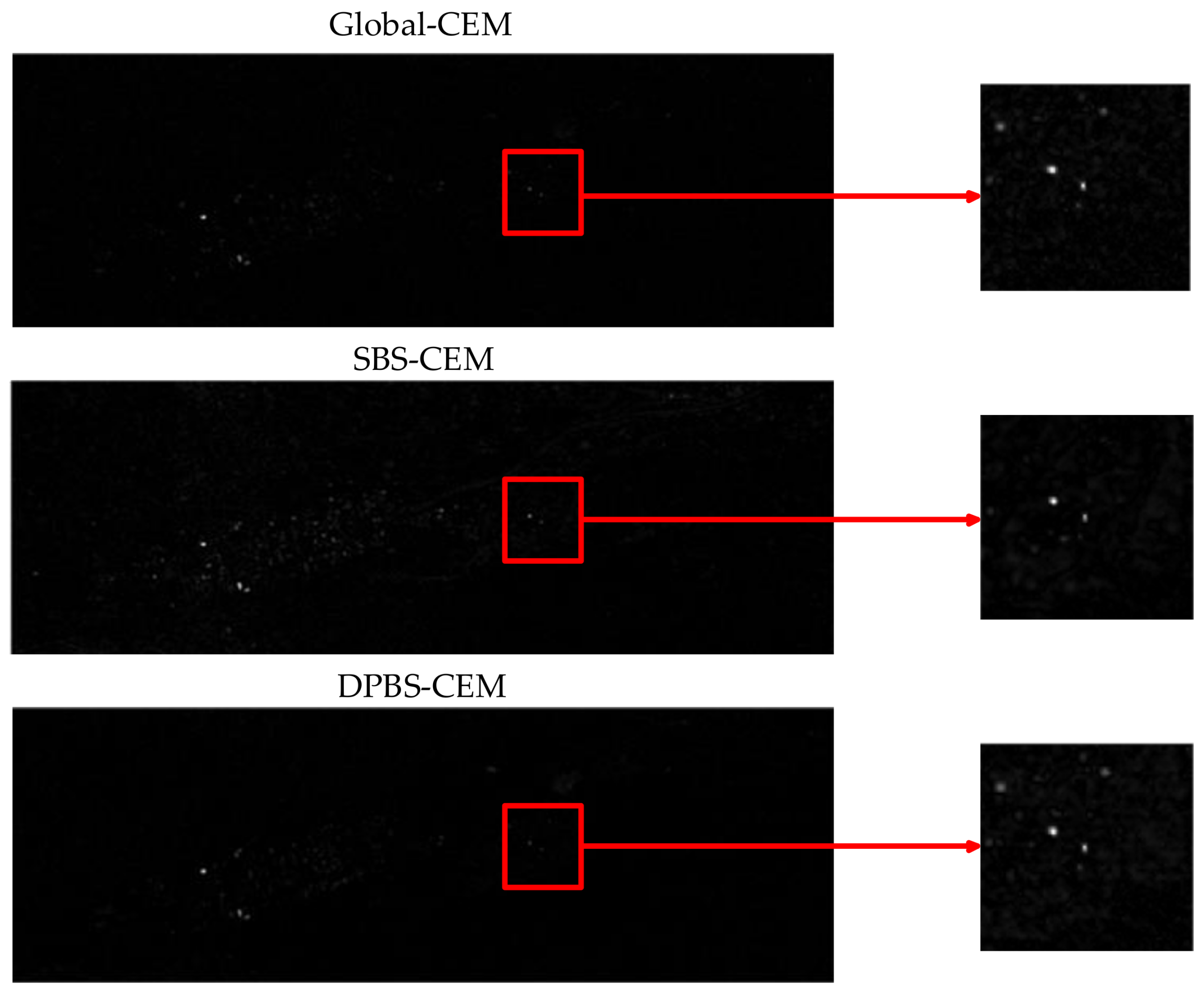
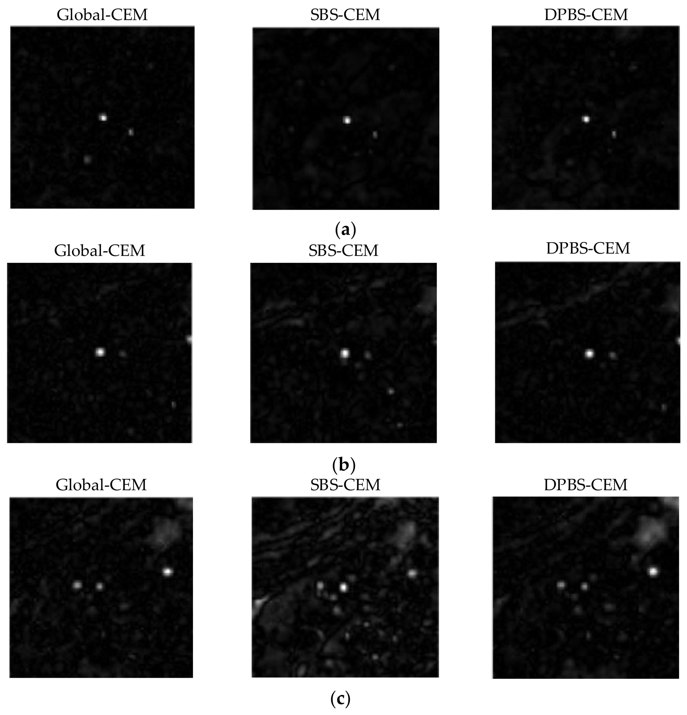
5.2. Analysis of Target Detection Accuracy
5.2.1. Detection Accuracy of TE1
5.2.2. Detection Accuracy of HyMap
5.3. Cross-Platform Performance Comparison
5.4. Performance Comparison between DPBS-CEM and SBS-CEM
6. Discussion
7. Conclusions
Acknowledgments
Author Contributions
Conflicts of Interest
Abbreviations
| HSI | Hyperspectral image |
| FPGA | Field programmable gate array |
| CEM | Constrained energy minimization |
| HLS | High-level synthesis |
Appendix A

| Directive | Description |
|---|---|
| #pragma HLS INTERFACE | Specifies how RTL ports are created from the function description. |
| #pragma HLS PIPELINE | Reduces the initiation interval by allowing the concurrent execution of operations within a loop or function. |
| #pragma HLS ARRAY_PARTITION | Partitions large arrays into multiple smaller arrays or into individual registers, to improve access to data and remove block RAM bottlenecks. |
| #pragma HLS UNROLL | Unroll for-loops to create multiple independent operations rather than a single collection of operations. |
| #pragma HLS DATAFLOW | Enable task level pipelining, allowing functions and loops to execute concurrently. Used to minimize interval. |
References
- Chang, C.I. Hyperspectral Imaging: Spectral Techniques for Detection and Classification; Kluwer Academic Publishers: Norwell, MA, USA, 2003. [Google Scholar]
- Ryan, J.P.; Davis, C.O.; Tufillaro, N.B.; Kudela, R.M.; Gao, B.C. Application of the hyperspectral imager for the coastal ocean to phytoplankton ecology studies in Monterey Bay, CA, USA. Remote Sens. 2014, 6, 1007–1025. [Google Scholar] [CrossRef]
- Dale, L.M.; Thewis, A.; Boudry, C.; Rotar, I.; Dardenne, P.; Baeten, V.; Pierna, J.A.F. Hyperspectral imaging applications in agriculture and agro-food product quality and safety control: A review. Appl. Spectrosc. Rev. 2013, 48, 142–159. [Google Scholar] [CrossRef]
- Zhang, B.; Wu, D.; Zhang, L.; Jiao, Q.; Li, Q. Application of hyperspectral remote sensing for environment monitoring in mining areas. Environ. Earth Sci. 2012, 65, 649–658. [Google Scholar] [CrossRef]
- Cloutis, E.A. Review article hyperspectral geological remote sensing: Evaluation of analytical techniques. Int. J. Remote Sens. 1996, 17, 2215–2242. [Google Scholar] [CrossRef]
- Chang, C.I. Real-Time recursive hyperspectral sample and band processing: Algorithm architecture and implementation. In Real-Time Recursive Hyperspectral Sample and Band Processing, 1st ed.; Springer: Berlin, Germany, 2017; pp. 123–156. ISBN 978-3-319-45170-1. [Google Scholar]
- Wang, Y.; Huang, S.; Liu, D.; Wang, H. A target detection method for hyperspectral imagery based on two-time detection. J. Indian Soc. Remote Sens. 2017, 45, 239–246. [Google Scholar] [CrossRef]
- Zou, Z.; Shi, Z. Hierarchical suppression method for hyperspectral target detection. IEEE Trans. Geosci. Remote Sens. 2016, 54, 330–342. [Google Scholar] [CrossRef]
- He, C.; Zhao, Y.; Tian, J.; Shi, P.; Huang, Q. Improving change vector analysis by cross-correlogram spectral matching for accurate detection of land-cover conversion. Int. J. Remote Sens. 2013, 34, 1127–1145. [Google Scholar] [CrossRef]
- Chaudhuri, S.; Chatterjee, S.; Katz, N.; Nelson, M.; Goldbaum, M. Detection of blood vessels in retinal images using two-dimensional matched filters. IEEE Trans. Med. Imaging 1989, 8, 263–269. [Google Scholar] [CrossRef] [PubMed]
- Yuhas, R.H.; Goetz, A.F.; Boardman, J.W. Discrimination among semi-arid landscape endmembers using the spectral angle mapper (SAM) algorithm. In JPL, Summaries of the Third Annual JPL Airborne Geoscience Workshop; NASA: Washington, DC, USA, 1992; pp. 147–149. [Google Scholar]
- Du, Q.; Ren, H.; Chang, C.I. A comparative study for orthogonal subspace projection and constrained energy minimization. IEEE Trans. Geosci. Remote Sens. 2003, 41, 1525–1529. [Google Scholar]
- Ren, H.; Chang, C.I. A target-constrained interference-minimized filter for subpixel target detection in hyperspectral imagery. In Proceedings of the Geoscience and Remote Sensing Symposium, Honolulu, HI, USA, 24–28 July 2000; pp. 1545–1547. [Google Scholar]
- Manolakis, D.; Marden, D.; Shaw, G.A. Hyperspectral image processing for automatic target detection applications. J. Lincoln Lab. 2003, 14, 79–116. [Google Scholar]
- Scharf, L.L.; Friedlander, B. Matched subspace detectors. IEEE Trans. Signal Process. 1994, 42, 2146–2157. [Google Scholar] [CrossRef]
- Harsanyi, J.C.; Chang, C.I. Hyperspectral image classification and dimensionality reduction: An orthogonal subspace projection approach. IEEE Trans. Geosci. Remote Sens. 1994, 32, 779–785. [Google Scholar] [CrossRef]
- Chen, Y.; Nasrabadi, N.M.; Tran, T.D. Sparse representation for target detection in hyperspectral imagery. IEEE J. Sel. Top. Signal Process. 2011, 5, 629–640. [Google Scholar] [CrossRef]
- Mittal, S.; Vetter, J.S. A survey of CPU-GPU heterogeneous computing techniques. ACM Comput. Surv. 2015, 47, 69. [Google Scholar] [CrossRef]
- Plaza, A.; Chang, C.I. Clusters Versus FPGA for parallel processing of hyperspectral imagery. Int. J. High Perform. Comput. Appl. 2008, 22, 366–385. [Google Scholar] [CrossRef]
- Wang, J.; Chang, C.; Cao, M. FPGA design for constrained energy minimization. Proc. SPIE 2004, 262–273. [Google Scholar] [CrossRef]
- Yang, B.; Yang, M.; Plaza, A.; Gao, L.; Zhang, B. Dual-mode FPGA implementation of target and anomaly detection algorithms for real-time hyperspectral imaging. IEEE J.-STARS 2015, 8, 2950–2961. [Google Scholar] [CrossRef]
- Gonzalez, C.; Bernabe, S.; Mozos, D.; Plaza, A. FPGA implementation of an algorithm for automatically detecting targets in remotely sensed hyperspectral images. IEEE J. Sel. Top. Appl. Earth Obs. Remote Sens. 2016, 9, 4334–4343. [Google Scholar] [CrossRef]
- Santos, L.; López, J.F.; Sarmiento, R.; Vitulli, R. FPGA implementation of a lossy compression algorithm for hyperspectral images with a high-level synthesis tool. In Proceedings of the 2013 NASA/ESA Conference on Adaptive Hardware and Systems, Torino, Italy, 24–27 June 2013; pp. 107–114. [Google Scholar]
- García, A.; Santos, L.; López, S.; Callicó, G.M.; Lopez, J.F.; Sarmiento, R. Efficient lossy compression implementations of hyperspectral images: Tools, hardware platforms, and comparisons. In Satellite Data Compression, Communications, and Processing X; International Society for Optics and Photonics: Bellingham, WA, USA, 2014. [Google Scholar]
- Domingo, R.; Salvador, R.; Fabelo, H. High-level design using Intel FPGA OpenCL: A hyperspectral imaging spatial-spectral classifier. In Proceedings of the 2017 IEEE 12th International Symposium on Reconfigurable Communication-Centric Systems-on-Chip (ReCoSoC), Madrid, Spain, 12–14 July 2017; pp. 1–8. [Google Scholar]
- Del Sozzo, E.; Solazzo, A.; Miele, A.; Santambrogio, M.D. On the automation of high level synthesis of convolutional neural networks. In Proceedings of the 2016 IEEE International Symposium on Parallel and Distributed Processing, Chicago, IL, USA, 23–27 May 2016; pp. 217–224. [Google Scholar]
- Guan, Y.; Liang, H.; Xu, N.; Wang, W.; Shi, S.; Chen, X. FP-DNN: An automated framework for mapping deep neural networks onto FPGAs with RTL-HLS hybrid templates. In Proceedings of the 2017 IEEE International Symposium on Field-Programmable Custom Computing Machines, Napa, CA, USA, 30 April–2 May 2017; pp. 152–159. [Google Scholar]
- Hager, W.W. Updating the inverse of a matrix. Siam Rev. 1989, 31, 221–239. [Google Scholar] [CrossRef]
- Chang, C.I.; Li, H.C.; Song, M.; Liu, C.; Zhang, L. Real-time constrained energy minimization for sub pixel detection. IEEE J.-STARS 2015, 8, 2545–2559. [Google Scholar]
- Chang, C.I. Real-Time Recursive Hyperspectral Sample Processing for Active Target Detection: Constrained Energy Minimization. In Real-Time Recursive Hyperspectral Sample and Band Processing, 1st ed.; Springer: Berlin, Germany, 2017; pp. 123–156. ISBN 978-3-319-45170-1. [Google Scholar]
- Nasrabadi, N.M. Regularized spectral matched filter for target recognition in hyperspectral imagery. IEEE Signal. Proc. Lett. 2008, 15, 317–320. [Google Scholar] [CrossRef]
- Wang, J.; Chang, C.I. Applications of independent component analysis in endmember extraction and abundance quantification for hyperspectral imagery. IEEE Trans. Geosci. Remote Sens. 2006, 44, 2601–2616. [Google Scholar] [CrossRef]
- Chang, C.I. Design of Synthetic Image Experiments. In Hyperspectral Data Processing: Algorithm Design and Analysis, 1st ed.; John Wiley & Sons: Hoboken, NJ, USA, 2013; pp. 103–113. ISBN 978-0-471-69056-6. [Google Scholar]
- Snyder, D.; Kerekes, J.; Fairweather, I.; Crabtree, R.; Shive, J.; Hager, S. Development of a web-based application to evaluate target finding algorithms. In Proceedings of the Geoscience and Remote Sensing Symposium, Boston, MA, USA, 6–11 July 2008; pp. II-915–II-918. [Google Scholar]
- Parker, D.R.; Gustafson, S.C.; Ross, T.D. Receiver operating characteristic and confidence error metrics for assessing the performance of automatic target recognition systems. Opt. Eng. 2005, 44, 097202. [Google Scholar] [CrossRef]
- Metz, C.E. Basic principles of ROC analysis. Semin. Nucl. Med. 1978, 8, 283–298. [Google Scholar] [CrossRef]


| Stage Number | Formula | Flop | Parallelism | Clock Cycles |
|---|---|---|---|---|
| 1 | L | L | ||
| 2 | 1 | L | ||
| 3 | L | L | ||
| 4 | L | L |
| Row1 | = 0.5A + 0.5B | = 0.5A + 0.5C | = 0.5A + 0.5K | = 0.5A + 0.5M |
| Row2 | = 0.5B + 0.5A | = 0.5B + 0.5C | = 0.5B + 0.5K | = 0.5B + 0.5M |
| Row3 | = 0.5C + 0.5A | = 0.5B + 0.5C | = 0.5C + 0.5K | = 0.5C + 0.5M |
| Row4 | = 0.5K + 0.5A | = 0.5K + 0.5B | = 0.5K + 0.5C | = 0.5K + 0.5M |
| Row5 | = 0.5M + 0.5A | = 0.5M + 0.5B | = 0.5M + 0.5C | = 0.5M + 0.5K |
| Row | Fourth Column | Fifth Column |
|---|---|---|
| 1 | = 0.5A + 0.5BKG | = 0.25A + 0.75BKG |
| 2 | = 0.5B + 0.5BKG | = 0.25B + 0.75BKG |
| 3 | = 0.5C + 0.5BKG | = 0.25B + 0.75BKG |
| 4 | = 0.5K + 0.5BKG | = 0.25K + 0.75BKG |
| 5 | = 0.5M + 0.5BKG | = 0.25M + 0.75BKG |
| Name | F1 | F2 | F3a | F3b | F4a | F4b |
|---|---|---|---|---|---|---|
| Size (m) | 3 × 3 | 3 × 3 | 2 × 2 | 1 × 1 | 2 × 2 | 1 × 1 |
| Fabric type | Red cotton | Yellow nylon | Blue cotton | Blue cotton | Red nylon | Red nylon |
| F1 | F2 | F3 | F4 | |
|---|---|---|---|---|
| Global-CEM | 0.9107 | 1 | 0.9067 | 0.9987 |
| SBS-CEM [18] | 0.9783 | 1 | 0.9862 | 0.9972 |
| DPBS-CEM | 0.9997 | 0.9999 | 0.9992 | 0.9994 |
| Platform | MATLAB (s) | C++ (s) | FPGA (s) |
|---|---|---|---|
| HyMap | 60.7378 | 58.135 | 0.1568 |
| SBS-CEM Units (G) | DPBS-CEM Units (Z) | Ratio | |
|---|---|---|---|
| Number of DSP48Es | 265 | 1396 | 5.27 |
| Number of Block RAM | 120 | 379 | 3.16 |
| Number of Slices | 12,088 | 58,167 | 4.81 |
| Number of Flip Flops | 28,245 | 217,958 | 7.72 |
| Number of LUTs | 21,730 | 111,073 | 5.11 |
| Average Ratio | – | – | 5.21 |
| Precision (Bit) | 32 | 34 | 36 | 38 | 40 | 48 |
|---|---|---|---|---|---|---|
| AUC | 0.2530 | 0.4779 | 0.5463 | 0.9997 | 0.9997 | 0.9997 |
| SBS-CEM | DPBS-CEM | Speedup | |
|---|---|---|---|
| Frequency (MHz) | 200 | 200 | 7.3× |
| Number of clock periods | 229,607,996 | 31,360,557 |
© 2018 by the authors. Licensee MDPI, Basel, Switzerland. This article is an open access article distributed under the terms and conditions of the Creative Commons Attribution (CC BY) license (http://creativecommons.org/licenses/by/4.0/).
Share and Cite
Lei, J.; Li, Y.; Zhao, D.; Xie, J.; Chang, C.-I.; Wu, L.; Li, X.; Zhang, J.; Li, W. A Deep Pipelined Implementation of Hyperspectral Target Detection Algorithm on FPGA Using HLS. Remote Sens. 2018, 10, 516. https://doi.org/10.3390/rs10040516
Lei J, Li Y, Zhao D, Xie J, Chang C-I, Wu L, Li X, Zhang J, Li W. A Deep Pipelined Implementation of Hyperspectral Target Detection Algorithm on FPGA Using HLS. Remote Sensing. 2018; 10(4):516. https://doi.org/10.3390/rs10040516
Chicago/Turabian StyleLei, Jie, Yunsong Li, Dongsheng Zhao, Jing Xie, Chein-I Chang, Lingyun Wu, Xuepeng Li, Jintao Zhang, and Wenguang Li. 2018. "A Deep Pipelined Implementation of Hyperspectral Target Detection Algorithm on FPGA Using HLS" Remote Sensing 10, no. 4: 516. https://doi.org/10.3390/rs10040516