Modeling Environments Hierarchically with Omnidirectional Imaging and Global-Appearance Descriptors


Department of Systems Engineering and Automation, Miguel Hernández University, 03202 Elx Alicante, Spain
*
Author to whom correspondence should be addressed.
†
Current address: Avda. de la Universidad, s/n. Ed. Innova, 03202 Elx Alicante, Spain.
‡
These authors contributed equally to this work.
Remote Sens. 2018, 10(4), 522; https://doi.org/10.3390/rs10040522
Submission received: 19 January 2018
/
Revised: 20 March 2018
/
Accepted: 23 March 2018
/
Published: 26 March 2018
(This article belongs to the Section Remote Sensing Image Processing)
Abstract
:In this work, a framework is proposed to build topological models in mobile robotics, using an omnidirectional vision sensor as the only source of information. The model is structured hierarchically into three layers, from one high-level layer which permits a coarse estimation of the robot position to one low-level layer to refine this estimation efficiently. The algorithm is based on the use of clustering approaches to obtain compact topological models in the high-level layers, combined with global appearance techniques to represent robustly the omnidirectional scenes. Compared to the classical approaches based on the extraction and description of local features, global-appearance descriptors lead to models that can be interpreted and handled more intuitively. However, while local-feature techniques have been extensively studied in the literature, global-appearance ones require to be evaluated in detail to test their efficacy in map-building tasks. The proposed algorithms are tested with a set of publicly available panoramic images captured in realistic environments. The results show that global-appearance descriptors along with some specific clustering algorithms constitute a robust alternative to create a hierarchical representation of the environment.
1. Introduction to Map Building Using Vision Sensors
Over the last few years, mobile robots have become a crucial technology to solve a variety of tasks. Creating an optimal model of the environment where they are moving is one of the most important abilities they must be endowed with, so that they can estimate its position and navigate towards the target points. With this aim, robots must be equipped with sensors that enable them to collect the necessary information to model the environment. In this work, the robot is equipped with a catadioptric vision sensor which provides it with omnidirectional images from the environment. Owing mainly to the large quantity of information they can capture with only one snapshot (360 around the camera axis), omnidirectional vision systems have become a popular option in the implementation of mapping algorithms such as the SLAM method presented by Caruso et al. [1], who prove that even at relatively low resolutions, the model built with omnidirectional images provides a good localization accuracy. Additionally, if the movement of the robot is contained in the floor plane, the models built from omnidirectional scenes would permit implementing localization algorithms which work correctly independently of the orientation of the robot. This is a key feature to obtain fully functional models.
Working with visual sensors entails some other difficulties, because omnidirectional images are high-dimensional data which may change substantially not only when the robot moves but also under other circumstances, such as changes in the lighting conditions. Also, realistic indoor environments are prone to the perceptual aliasing problem, that is, images which have been captured from different positions may have a similar appearance, which would lead to confusion about the position of the robot. Taking these facts into account, a processing step is necessary to extract relevant and distinguishable information from the scenes which is able to cope with these events. This processing step must lead to compact visual descriptors that permit building useful models with computational efficiency. Traditionally, researchers have made use of methods based on the extraction, description and tracking of relevant landmarks or local features, such as SIFT (Scale Invariant Feature Transform), SURF (Speeded-Up Robust Features) or ORB (Oriented FAST and Rotated BRIEF) features [2,3,4]. They can be considered mature methods, and some analyses of their performance can be found in the literature, such as the one developed by Jiang et al. [5], who make a comparative evaluation in stereovisual odometry tasks. More recently, a new family of methods that process the image as a whole, with no local feature extraction, have emerged. These global-appearance methods build one unique, compact descriptor per scene, and a number of alternatives can be found in the literature [6,7,8]. Since each image is represented with a sole descriptor, these methods usually lead to more simple models of the environment and relatively straightforward localization algorithms, based on the direct comparison between pairs of descriptors. Nevertheless, they contain no metrical information and therefore, they have been used typically to construct topological models, which have proved to be enough for most applications [9,10].
In this work, a framework to create a topological hierarchical model of the environment is proposed and tested. In the literature, some developments can be found about hierarchical mapping. Galindo et al. [11] present a method to build a map that includes two hierarchies, a spatial one, which consists of a grid map obtained from range sensors, and a semantic one, constructed from the data captured by a set of sonars and a video camera. Also, Pronobis and Jensfelt [12] develop a hierarchical approach to categorization of places, using a variety of input data, and they cluster places using a door detector. In our work, only visual information is used. A set of images captured from several points of view of the a-priori unknown environment are available. Starting from them, a hierarchical map is created, by arranging the information into several layers, with different degrees of detail: (a) one high-level map, which reflects the general structure of the environment (that is, the rooms that compose it); (b) one or more intermediate-level maps, containing information on the different regions that exist in each room; and (c) a low-level map which contains the original set of images and the connectivity relationships between them. The creation of the high-level and intermediate-level maps requires compacting the visual information, trying to extract common patterns that permit organizing it correctly. In this field, some authors have proposed data-compression strategies to build efficient maps based on local features [13,14,15]. Amongst the compression methods, clustering algorithms can be used to compact the information because they are potentially able to group the visual information into several clusters containing visually similar scenes, and represent each cluster with a representative instance. Previous works have made use of such algorithms to create visual models of an environment, using local features, such as Zivkovik et al. [16], Valgren et al. [17] and Stimec et al. [18]. Ideally, to create useful maps, the clustering algorithm should group images that have been captured from geometrically close positions. However, visual aliasing could lead to errors in the model if only visual information is used.
The main contribution of this work consists in developing a comparative evaluation of several well-known global-appearance descriptors to create the hierarchical model. Also, some clustering methods are tested and their performance to create each layer of the map is assessed. Since only visual information and global-appearance descriptors are used, the framework will lead to purely topological models and it must be able to cope with the visual aliasing phenomenon. A publicly available set of images, captured in a realistic indoor environment, is used to test the algorithms developed and to tune all the parameters involved. Finally, to prove the validity of the mapping method, the hierarchical localization problem is also solved and its performance is compared with the performance of an absolute localization method.
The current work continues and expands the scope of the research presented in [19], where a comparative evaluation between some global description methods is carried out to obtain a low-level map and to create the topological relationships between the images of this level. Now, this evaluation is extended and generalized, and a method is proposed to create hierarchical maps which arrange the information more optimally, into several layers, which would permit an efficient localization subsequently.
The remainder of the paper is structured as follows. In Section 2, a succinct outline of the global-appearance approaches that will be used throughout the paper is made. After that, Section 3 presents the framework proposed to create hierarchical maps and the clustering methods used to compact the visual information in the high-level layers. Section 4 presents the set of experiments that have been conducted to validate the proposal. To conclude, a final discussion is carried out in Section 5.
2. State of the Art of Global Appearance Descriptors
In this section, some methods to describe the global appearance of a set of scenes are presented. The performance of these methods in hierarchical mapping will be evaluated throughout the subsequent sections. Five families of techniques are used to obtain the global-appearance descriptors in this work: the discrete Fourier transform (Section 2.1), principal component analysis (Section 2.2), histograms of oriented gradients (Section 2.3), the gist of the scenes (Section 2.4) and convolutional neural networks (Section 2.5). A detailed description of the methods can be found in [19,20].
2.1. Fourier Signature
The Fourier signature is a method to describe the global appearance of an image and was initially proposed in [21,22]. It consists of calculating the discrete Fourier transform of each row of the initial image. The result is a transformed, complex matrix (v is the frequency variable) where the most relevant information is concentrated on the first components of each row. Additionally, the last components are prone to be contaminated by the possible presence of high-frequency noise in the original image, so only the first columns are usually retained, having a compression effect. Furthermore, the matrix can be decomposed into a magnitudes matrix and an arguments matrix . The magnitudes matrix contains information on the overall structure of the image. Also, if the image is panoramic, then is invariant against changes of the robot’s orientation in the ground plane and can be used to estimate these changes, thanks to the shift theorem of the discrete Fourier transform [22]. Considering this, the magnitudes matrix can be considered as a global feature that describes the appearance of the environment as observed from the capture point of the image . This matrix can be arranged to compose a vector , where is the number of columns retained in the magnitudes matrix, and is an important parameter whose impact upon the mapping process must be evaluated.
2.2. Principal Component Analysis
Principal component analysis (PCA) constitutes a classical way to extract the most relevant information from a set of n images [23]. Each image can be considered as a point in a multidimensional space . This way, any classical PCA approach, such as the one proposed by Turk and Pentland [24], can be used to build a transformation matrix that permits projecting each point onto a new, lower-dimensional space. Each transformed point is known as a projection, and is the number of PCA features retained (those that contain the most relevant information). The use of such analysis in mapping and localization is quite limited mainly because the projections are not invariant against changes of the robot’s orientation in the ground plane, even if panoramic images are used. This is why Jogan and Leonardis [25,26] developed the concept of eigenspace of spinning images. When building the transformation matrix , they consider a set of rotated versions of each initial panoramic image, what permits including in the model some information about all the possible orientations the robot could have in a specific point of the environment. Taking advantage of the properties of these images, they decompose the original problem into a set of lower-order problems. Once the process finishes, the map is composed of (a) one descriptor per original panoramic image, , which are the position descriptors, since they are invariant against rotations of the robot; (b) one phase vector per image, , which permit calculating the orientation of the robot; and (c) the transformation matrix , where is the number of main eigenvectors retained. The two most relevant parameters in this process are and . On the one hand, the higher is, the more information on the robot’s orientation is included in the model, but the slower is the process to build it. On the other, the higher is, the more information is retained, and if , all the information contained in the original set of scenes is kept. This can be counter-productive, as the most relevant and distinguishing information is in the first components. Finally, despite being a mathematically optimized process, it is still computationally very expensive. Owing to this, the eigenspace of spinning images has been used typically to model small environments, with a reduced number of views. Throughout the paper, this method will be referred to as rotational PCA.
2.3. Histogram of Oriented Gradients
The histogram of oriented gradients (HOG) method proposes describing the appearance of one image through the orientation of the gradient in local areas of it. Originally developed by Dalal and Triggs [27] to perform people detection, it has scarcely been used in the modeling of controlled and relatively small environments [28]. The method used in the present paper is fully described in [7], where HOG is redefined to create two global-appearance descriptors of a panoramic image: a position descriptor, which is invariant against rotations of the robot in the ground plane, and an orientation descriptor, which permits calculating the relative angle rotated by the robot. On the one hand, the position descriptor is built by dividing the panoramic image into a set of horizontal cells. A histogram with b bins per cell is built, from the information of the gradient orientation of each pixel within it, and all the histograms are arranged in a vector, to compose the descriptor. On the other hand, the orientation descriptor is obtained after dividing the image into a set of overlapped vertical cells and obtaining one histogram per cell.
2.4. Gist of the Images
This concept was developed by Oliva et al. [29,30] to obtain low-dimensional descriptors from the global appearance of the images, inspired by the human process to recognize scenes. More recent works have established a synergy between it and the prominence concept, which tries to model the properties that make a pixel to stand out with respect to its neighborhood. It has led to descriptors built from the intensity, orientation and color information [31]. Some authors have used these concepts in mapping and localization tasks [32,33], by calculating the gist descriptor in local areas of the images. In the present work, we use an implementation of the gist descriptor, based on orientation information, which reflects the global appearance of the scene. A complete explanation can be found in [7]. This implementation leads to one position descriptor and one orientation descriptor per panoramic image. In brief, several Gabor filters are applied to the panoramic image, with m evenly distributed orientations and 2 resolution levels. The information is then grouped into (a) horizontal blocks (by calculating the average value of each block) and arranged into a vector to compose the position descriptor , and (b) vertical blocks with overlapping to create the orientation descriptors .
2.5. Descriptor Based on the Use of Convolutional Neural Networks
In recent years, the success of deep-learning techniques has led to an increase of the use of convolutional neural networks (CNN) as an alternative to carry out object recognition from the information contained in digital images, with no need for extracting local features from them. These neural networks work with the images globally, and their main purpose consists of extracting information from them, for example, to carry out a classification or object-detection task. Firstly, the network has to go under a learning process, in which a set of training images, whose category is previously known, is presented to the network. Thanks to this, the neurons’ weights and biases are tuned. Secondly, once trained, when an image is presented to the network to extract information from it, the network starts obtaining the most appropriate description of the image. Several intermediate descriptors may be obtained, depending on the number of layers in the network.
Convolutional neural networks were initially proposed and developed to carry out object recognition from digital images. A variety of network architectures can be highlighted owing to their good performance in this task, such as AlexNet [34], GoogleNet [35] or VGG-16 [36]. More recently, CNNs have evolved and some alternatives can be found to develop categorization of visual scenes into types of place. When an image is presented to these networks, they generate visual descriptors which are useful to solve, subsequently, the categorization task. The descriptors provided by the last layers of these convolutional networks are specially relevant for the present work, because they can be considered as global features that contain relevant information from the original image. In the early stages of this technology, the networks were trained with a wide variety of input data to carry out object recognition subsequently. However, in the last few years, some CNN frameworks have been proposed that include networks previously trained in scene-categorization tasks [20]. We propose using an Alexnet CNN architecture trained on 205 scene categories of a places database with about million images [37]. We make use of this previously trained network with the objective of obtaining a descriptor for each of the images considered in this work to carry out hierarchical mapping. More concisely, we consider two alternatives to describe each image: the descriptor provided by the layer fc7 of the network, which contains 4096 components (that is, ), and the descriptor provided by the layer fc8, which contains 205 components (). These are the last two fully connected layers of the network.
3. Creating a Hierarchical Map from a Set of Scenes
This section concentrates on the creation of a multi-layer hierarchical map from a set of images captured along the environment. A clustering approach will be used to group sets of images together and create each topological layer in the hierarchical map. Firstly, a general description of the process and the contents of the map are outlined in Section 3.1. After that, the clustering algorithms used throughout the paper are presented in Section 3.2.
3.1. Creating the Low-Level and the High-Level Topological Maps
The objective of this paper consists of developing strategies to create visual hierarchical maps, using only the information contained in a set of images, which have been captured from several points of view of a multiroom environment, to cover it completely. This way, the visual information must be grouped into several layers, by means of any clustering algorithm, with the objective of enabling a subsequent localization in an efficient way.
To optimize the task, this work proposes building a hierarchical topological map that arranges the information into three layers:
- (a)
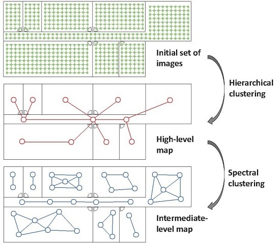
- Low-level map. It represents the images captured within the environment and the topological relationships between them. Figure 1a shows the low-level map of a sample generic environment. The green squares represent the capture points of the images.
- (b)
- Intermediate-level map. It represents groups of images that have been captured from points of the environment that are geometrically close among them. Every group will be characterized by a representative image, which identifies the group, and is fundamental to carry out the hierarchical localization process. Figure 1b shows an example. The intermediate-level map is composed of several clusters (whose representatives are shown as blue circles in this figure) and connectivity relationships among them.
- (c)
- High-level map. It represents the rooms that compose the environment and the connectivity relationships between them (Figure 1c). Ideally, the high-level map contains as many clusters as rooms in such a way that every cluster contains all the scenes captured within each room.
The steps we propose to build the complete hierarchical map are:
- Grouping images together to create the high-level map. The algorithm starts from the complete set of images, captured by the robot when it goes through the entire environment to map. Making use of a clustering algorithm, these images must be grouped together in such a way that the resulting clusters coincide with the rooms of the environment. In this step, the ability of both the description and the clustering algorithms will be tested to solve the task. Also, the necessary parameters will be tuned to optimize the results. The main complexity of this task lies in the visual aliasing phenomenon, which may result in a mix-up between scenes captured from different rooms (that is, they can be assigned to the same cluster). This analysis is performed in Section 4.3.
- Creating groups with the images of each room to obtain the intermediate-level map. This step is repeated for each of the clusters created in the previous step, taking as initial data the images that each specific cluster contains. Using another clustering algorithm, these images must be grouped together in such a way that the resulting clusters contain images captured from geometrically close points. This is a complex problem, as the only criterion to make the groups is the similitude between the visual descriptors, which are the only data available. Once again, a series of experiments will be conducted to assess the validity of each description and clustering method to solve the task. To validate the results, we will check whether the clusters created with the visual similitude criterion actually contain images that have been captured from geometrically close points. This problem is analyzed in detail in Section 4.4.
- Setting topological relationships between the images and the cluster representatives. The objective is to establish these relationships in order to obtain a complete and functional map at each level that represents the connectivity between capture points and furthermore, that includes information on the relative distance between these points.
This is an advantageous approach to create the model of the environment from the point of view of the subsequent localization task, which can be carried out hierarchically, with a computationally efficient process. This way, firstly, the different layers permit carrying out the localization task in a hierarchical way. Secondly, the topological relationships permit navigating towards the target points. About the localization process, when the robot is at an unknown position, it will capture an image, describe it and compare the descriptor with the representatives of the clusters that compose the high-level map. As a result, a coarse localization is obtained in one of the rooms of the environment. After that, the descriptor is compared with the representatives of the intermediate-level map that belong to this room, and a more fine localization in an area of the environment is obtained. To finish, the descriptor is compared with the images of the low-level map that belong to the winning cluster of the intermediate-level map, obtaining an accurate estimation of the position. Section 4 shows how the proposed model can be used to solve the localization problem hierarchically, and the accuracy and computational cost of this process, comparing it to an absolute localization process (with no hierarchical model available).
The third step was developed in detail in [19], where a method based on a physical system of forces was proposed to establish topological relationships between the capture points of a set of images, using only the visual information to this purpose. The method proved to work correctly and efficiently with a set of images captured in a real environment and under real working conditions. Considering this, in this paper, the first and second steps will be addressed. The same dataset will be used in the experimental section (Section 4) to test the proposed methods. The next subsection lays out these problems and our approach to them.
3.2. Compacting Visual Models Using a Clustering Approach
As presented in the previous subsection, the creation of the different layers of the hierarchical map is addressed from a clustering point of view. Generally speaking, the clustering algorithms enable us to handle massive amounts of data to extract some relevant information from them, in such a way that their analysis is more systematic. These algorithms classify a set of entities or data vectors. Each cluster is characterized by the common attributes of the entities it contains. In this application, the entities are the position descriptors of the scenes, which have, in general, l dimensions each (as specified in Section 2 for each description method). To build a topological model of the environment, it is necessary to choose an appropriate clustering method and test the feasibility of each description method and the influence of its size upon the correctness of the results.
An exhaustive compilation of clustering algorithms can be found in the works of Everitt et al. [38]. In the present work, two families of methods will be used and tested: hierarchical and spectral clustering algorithms. To start with, a more detailed description of these algorithms will be included, and then the experiments will be addressed.
In all the cases, the input data is a set of scenes which have been captured from several positions of the environment to map. A global-appearance position descriptor is calculated from each image and, as a result, a set of visual descriptors is available, where, in general, . The poses (position and orientation) of the capture positions are also known, . However, this information will be used only as ground-truth data to assess the correctness of the results; purely visual information is proposed to be used during the mapping and localization processes.
To create each layer of the hierarchical map, a clustering approach will be used. The initial dataset will be divided into k clusters such that:
Once this process has been carried out, a representative descriptor will be calculated for each cluster, so that a layer of the model will be composed of the set of representatives . Ideally, the clusters must contain images that were captured from geometrically near positions. Nevertheless, in a real application, this may not be true due to the visual aliasing phenomenon. Considering both this phenomenon and the high dimensionality of the data, classical clustering algorithms, such as k-means, would not work optimally. Instead, the algorithms presented in the next two subsections will be tested.
3.2.1. Hierarchical Clustering
Hierarchical clustering algorithms [39] group the data together, step by step, into a hierarchical clusters’ tree or dendrogram. To start with, each entity is considered a cluster. Then, in each iteration, the two most similar clusters are gathered to create a new cluster in the next level. The process finishes when a cluster that contains all the entities has been created. This process permits deciding the most appropriate number of clusters for one specific application. To perform a hierarchical clustering, the next algorithm has to be followed:
- Initialization:
- (a)
- The initial set of clusters is chosen as .
- (b)
- . This is the initial distances’ matrix of the dataset , a symmetric matrix where each component is .
- (c)
- .
- Repeat (until all the entities are included in a unique cluster):
- (a)
- .
- (b)
- Among all the possible pairs of clusters in , the pair is detected.
- (c)
- Merge and produce the new set of clusters .
- (d)
- The distances’ matrix is defined from by deleting the two rows and columns that belong to the merged clusters, and adding a new row and column that contain the distance between the new cluster and the other clusters that remain unchanged.
- Finalization:
- (a)
- Once the tree is built, a cutting level is defined, to decide the final division into clusters.
- (b)
- The branches of this level are pruned and all the entities that are under each cut are assigned to an individual cluster.
Usually, this kind of algorithm is implemented on the grounds of matrix theory. In every iteration of the clustering algorithm t, the two most similar clusters are merged to create a new cluster. There are several criteria that permit calculating the distance between the new cluster (which results from merging the two clusters and ) and a previous cluster . Depending on how we define this distance, a specific modality of the hierarchical clustering is obtained. Table 1 shows the most common expressions that can be used to calculate this distance. In this table, and are the cardinal numbers of the clusters and , respectively, is the p-th entity in cluster , and is the q-th entity in cluster .
Furthermore, to calculate the distance between each pair of entities, several distance measurements can be used. In the experiments, the performance of the following classical distance measures will be evaluated: (1) the cityblock or Manhattan distance ; (2) the Euclidean distance ; (3) a correlation distance, which is obtained from the Pearson correlation coefficient of the two vectors (Equation (2)); (4) a cosine distance, which is obtained from the inner product of the two normalized vectors (Equation (3)); (5) a weighted distance (Equation (4)), which weights more the difference of the first components of both vectors; and (6) a square-root distance, (Equation (5)), which was proposed by [40] to be used in clustering applications with highly dimensional data.
where , and is the component of the vector .
Dendrograms constitute a powerful way to represent the sequence of clusters that an agglomerative algorithm produces at each step t. As an example, let us suppose that a set of data is initially available . These data have been obtained by calculating the Fourier signature of seven panoramic scenes captured from three different rooms. Making use of the correlation distance, the distances’ matrix is calculated (Equation (6)). In this matrix , each component represents the distance . Considering this matrix, the dendrogram that reflects the hierarchical clustering of the dataset can be depicted, as Figure 2a shows.
In the first step of the clustering algorithm, and are grouped together. The height of the horizontal branch that joins them is . This is the first group made by the algorithm, since these are the two entities that are the most similar. In the second step, and are grouped together. Thirdly, the algorithm groups and and then, in the fourth step, is assembled to the group , . The algorithm continues and naturally finishes when all the entities are joined into a unique cluster.
The height difference between every horizontal line and the one that is directly above gives us an idea of how natural or forced the creation of this step’s cluster has been. For example, the height difference between the branches created at steps 3 and 4 is relatively small. This means that the distance between the two clusters that have been joined to create a unique cluster is small, so this new cluster has been created in a natural fashion. However, the height difference between the steps 4 and 5 is relatively high, which indicates that the cluster created after the fifth step is forced; two clusters that are relatively different have been grouped together to create a new, unnatural cluster. Once the dendrogram has been built, to obtain the final set of clusters, it must be cut through a specific level. Choosing correctly this level is essential to obtain a set of clusters that represent in a natural way the input data. By choosing the cutting level shown in Figure 2b, clusters will be obtained which, additionally, constitutes a natural way to represent the data, as the line cuts vertical branches that are relatively high.
Once the dendrogram is built, it is advisable to study whether it represents the input data in a natural fashion. As presented in the previous paragraph, in a hierarchical clusters’ tree, in a specific iteration, two objects are grouped together to create a new cluster. The height of the branch created in this step represents the distance between the two clusters that contain these two objects. This height is known as the cophenetic distance between the two objects. A possible way to measure how well the tree represents the original data consists of comparing the cophenetic distances with the distances among the entities, which are stored in the distances’ matrix . In this work, we calculate the Spearman’s rank correlation between the distances among entities and the cophenetic distances. The more similar this coefficient is to 1, the more naturally the dendrogram represents the initial data.
Finally, once the cutting level has been selected and therefore the data have been split into clusters, the consistency of the clusters should be evaluated. To this purpose, the height of each branch can be compared with the heights of the neighbors that are situated beneath. If the height of one specific link is approximately equal to the height of the links below it, that indicates that there is no distinctive separation between the objects grouped in this level of hierarchy. This means that these links have a low consistency, and pruning them would lead to unnatural clusters. In the same way, inconsistent links point out the limit of a natural division of the dataset. The relative consistency of each link in a hierarchical clustering tree can be quantified through an inconsistency coefficient . This value is the result of comparing the height of the links situated in the pruned level with the average height of the links beneath it. Therefore, it is a measurement of the consistency of a specific division into k clusters from the original data. In each experiment, this coefficient has been normalized to take a maximum value equal to 1. This way, the higher this coefficient is, the more natural the final clusters are.
3.2.2. Spectral Clustering
The algorithms based on spectral clustering have proved to perform successfully with high-dimensional data [41], including images [17,18]. The implementation used in this work was proposed by Ng et al. [42].
The spectral clustering algorithms take the mutual similitude among all the entities into account. This is why they have proved to be more effective than traditional methods, which only consider the similitude between each entity and the k representatives. The algorithm starts obtaining the similitude between each pair of entities to build the similarity matrix , where:
The input to this algorithm is this matrix and the number of clusters k. The algorithm consists of the following steps:
- Calculate a diagonal matrix from the similarity matrix: .
- Obtain the Laplacian matrix .
- Diagonalize the matrix and arrange the k main eigenvectors (those with the largest eigenvalues) in columns, to compose the matrix .
- Normalize the rows of to create the matrix .
- Perform a k-means clustering, considering as entities the rows of . The outputs are the clusters .
- The outputs of the spectral clustering algorithm are the clusters such that .
The diagonalization involved in the third step may be computationally expensive when the number of entities n is very high. One possible solution to this problem consists of cancelling some of the components of the similitude matrix, to obtain a sparse matrix, and using sparse-matrix methods to obtain the required eigenvectors [41]. To do that, in the matrix , only the components such that j is among the t nearest neighbors of i or vice versa, t being a low number, are retained in this work. After that, the Lanczos/Arnoldi factorization is used to obtain the first k eigenvectors of the Laplacian matrix . Once the clusters have been created, the representatives are obtained as the average visual descriptor of all the descriptors included in each cluster.
To conclude this section, Figure 3 shows the block diagram of the framework proposed to create a hierarchical model of the environment, with the purpose of clarifying the goal of the subsequent experimental sections. This is the set of operations that will be carried out to obtain a hierarchical map in the next section.
4. Experiments
In this section, a comparative evaluation is carried out to test the performance of the two clustering methods and the five description approaches in the hierarchical mapping problem. Firstly, the sets of images used to develop the experiments are described. Secondly, the preliminary experiments that permit selecting the appropriate clustering method for each task are outlined. After that, the two main experiments are addressed: the creation of the high-level and the intermediate-level maps.
4.1. Sets of Images
Throughout this section, some publicly available sets of images captured by Möller et al., and described in [43], are used. They are composed of several groups of panoramic gray-scale images, captured on a regular grid in several spaces of Bielefeld University and rooms of an apartment. A robot, ActivMedia Pioneer 3-DS, with a catadioptric system mounted on it, was used to capture the images. The catadioptric system consists of an ImagingSource DFK 4303 camera pointing towards an Accowle Wide View hyperbolic convex mirror. The rooms used to perform the experiments in this paper and the main features of the images are shown in Table 2. It is worth highlighting the fact that the capture points of the images form a regular grid whose size is different for each room (the higher the size of the room, the longer the distance between capture positions). Also, the area of each room is substantially different to the others. This permits testing the validity of the algorithms independently of these features. These sets of images are referred to as the Bielefeld set throughout the remainder of the paper.
4.2. Preliminary Experiments
Before conducting a complete bank of experiments, preliminary tests were carried out to select the most useful clustering algorithm to solve each task. Firstly, the high-level clustering task was addressed, with the objective that the clusters coincide with the rooms of the environment. The preliminary tests performed with the Bielefeld set show that either pure k-means or the spectral algorithm are not useful to separate correctly the images that compose the four rooms. However, the hierarchical algorithm has provided, in general, relatively accurate results in this task, so it is worth studying its performance in depth and trying to tune the parameters to optimize the process. As an example, Figure 4 shows the results obtained after a global clustering using the Bielefeld set, gist as description method and the spectral algorithm. This figure shows that the kitchen and one area of the hall are grouped together into the same cluster, and also, some of the images of the laboratory are classified as belonging to the living room. Such a result was achieved only after a process to tune the parameters to optimize the results, and it was not possible to improve it. Meanwhile, the experiments carried out with the hierarchical algorithm showed, in general, relatively good results. This is why this algorithm will be analyzed in detail in Section 4.3.
As for the creation of the intermediate-level map, the objective is that the algorithm groups together images that have been captured from geometrically close positions within each room. The preliminary tests have shown the inability of the hierarchical algorithm to solve this task. As an example, Figure 5 shows the result obtained after applying the hierarchical clustering algorithm to obtain the intermediate-level maps in the kitchen and the laboratory of the Bielefeld set. When this experiment was repeated in different rooms, it tended to create one cluster containing a high number of images, and some other clusters which had very few images or even a unique image. This behavior was almost independent of the configuration of the parameters. However, the experiments carried out with the spectral clustering showed a more consistent and more balanced separation, both considering the number of scenes per cluster and the geometrical closeness between capture points. The use of this algorithm in the intermediate-level mapping will be studied in Section 4.4.
Considering these preliminary tests, the hierarchical algorithm will be the reference method for the creation of the high-level model and the spectral one for the intermediate-level layer (as the block diagram in Figure 3 shows). In the next two subsections, a comparative evaluation of the performance of both algorithms is presented, considering the impact of the most relevant parameters upon the results (both the parameters of the descriptors and those of the clustering method).
4.3. Experiment 1: Creating Groups of Images to Obtain a High-Level Map
To make an exhaustive analysis of the hierarchical clustering method in the creation of a high-level map, the influence of the next parameters will be assessed.
- Image description method. The performance of the five methods presented in Section 2 and the impact of their parameters is assessed: (number of columns retained) in the Fourier signature; (number of PCA components) and (number of rotations of each panoramic image) in the case of rotational PCA; (number of horizontal cells) in the HOG descriptor; (number of horizontal blocks) and m (number of Gabor masks) in gist; and finally, the descriptors obtained from the layers fc7 and fc8 in CNN.
- Method to calculate the distance . All the traditional methods in hierarchical clustering (Table 1) have been tested:
- -
- Single. Method of the shortest distance.
- -
- Complete. Method of the longest distance.
- -
- Average. Method of the average unweighted distance.
- -
- Weighted. Method of the average weighted distance.
- -
- Centroid. Method of the distance between unweighted centroids.
- -
- Median. Method of the distance between weighted centroids.
- -
- Ward. Method of the minimum intracluster variance.
- Distance measurement between descriptors. All the distances presented in Section 2 are considered in the experiments. The notation used is:
- -
- . Cityblock distance.
- -
- . Euclidean distance.
- -
- . Correlation distance.
- -
- . Cosine distance.
- -
- . Weighted distance.
- -
- . Square-root distance.
To analyze the correctness of the results provided by each experiment, the next data will be shown on the figures: (a) the accuracy of the classification; (b) how good the dendrogram represents the original entities; and (c) the consistency of the final clusters. Firstly, to calculate the precision of the classification, the NMI (normalized mutual information) algorithm has been used. It obtains the confusion matrix of the resulting groups and, from the information of the principal diagonal (correctly classified entities) and the rest of the information, it provides us with an index c that takes values in the range and which indicates the accuracy of the resulting clusters. In this application, the value 1 indicates that the resulting clusters reflect perfectly the rooms that compose the environment. The lower this value is, the more mixed the information is in the resulting clusters (that is, images captured from several rooms are classified into the same cluster). Secondly, the correlation between the cophenetic distances and the distance among entities is obtained to estimate how naturally the dendrogram represents the visual data. High values indicate that the dendrogram build during the clustering process reflects faithfully the descriptors of the original scenes. Thirdly, the consistency of the final clusters is evaluated through the inconsistency coefficient , as presented in Section 3.2.1.
Figure 6 shows the results obtained with the Fourier signature, using (a) , (b) and (c) components per row in the magnitudes’ matrix. The blue bars show the accuracy of the classification c, the red tendency is the correlation coefficient and, finally, the green tendency reflects the inconsistency coefficient . The value of the inconsistency coefficient has been normalized to the interval . The higher this coefficient is, the more natural is the final division into clusters. These figures show that the best results are those provided by the shortest distance method (single). Nevertheless, the maximum accuracy is under in all the cases. Analyzing this method in depth, if we increase (size of the descriptor), it leads to more consistent trees, because there is a general improvement in the correlation coefficient. However, the accuracy of the classification does not change as the size of the descriptor increases. This is a general effect that can be observed in Figure 6; increasing (size of the Fourier signature descriptor) does not lead to a clear improvement of the classification results. The centroid and median methods tend to present especially unsuccessful classification results. As a conclusion, the Fourier signature has not been able to create clusters that separate completely and accurately the rooms of the Bielefeld dataset while creating the high-level map.
Next, the Figure 7 shows the results obtained with the rotational principal component analysis, considering that the number of eigenvectors is and the number of rotations is (a) , (b) and (c) . In this experiment, the size of the descriptor is kept constant because preliminary experiments showed that this parameter had little influence on the results. The results obtained with rotational PCA are somewhat similar to those obtained with the Fourier signature. Figure 7 shows that the correlation distance () along with the single method provides an accuracy near 1. However, in this case, the correlation coefficient has a significantly low value. It indicates that the dendrogram does not reflect well the original visual data. Therefore, the clustering process has not been carried out in a natural fashion.
The next experiment has been carried out with the HOG descriptor. Figure 8 shows the results obtained when considering: (a) ; (b) ; and (c) horizontal cells. Further experiments considering a higher number of cells have shown no improvement. These figures show that the results obtained with the cell are predominantly unsuccessful. The results of the single method stand out due to their wrongness. Nevertheless, the cosine method distance () along with the methods weighted, centroid and Ward, provide remarkably good results, but they do not arrive at success rate, and the correlation takes comparatively low values in the three cases. Therefore, considering only the cell leads to a descriptor that does not contain distinctive-enough information to carry out the global mapping process successfully. Notwithstanding that, a clear improvement is shown when the number of cells increases and very accurate results are obtained when considering cells. With this configuration, several experiments have provided an accuracy equal to , with relatively good correlation coefficients (around ) and inconsistency coefficients near 1. This indicates that this cluster division is not only perfect but also consistent. The images captured in each room have been assigned to separate clusters, and this division reflects the visual input data in a natural way. It is worth highlighting the performance of the methods single and weighted (except when using the correlation distance ) and the Ward method.
After that, the results obtained with the gist descriptor are shown. In this case, the influence of the two main parameters of the descriptor is assessed: the number of horizontal blocks and the number of Gabor masks m. On the one hand, Figure 9 shows the results obtained when considering the gist descriptor, masks and (a) ; (b) ; and (c) blocks. On the other hand, Figure 10 shows the results obtained with masks and (a) ; (b) ; and (c) blocks. From Figure 9 and Figure 10, several conclusions can be reached. First, the number of masks m is of utmost importance to obtain accurate groups. In general, the results obtained with are better than those obtained with . Second, the influence of the number of horizontal blocks is not remarkable. Some methods, along with several specific distances, show a higher accuracy when the number of cells increases, but this is not usually accompanied by an improvement of the correlation and inconsistency coefficients. Third, the method of the longest distance (complete) does not perform well, independently of the distance measure used. Finally, when gist is used, the best absolute results are obtained with masks and (a) single method and cityblock distance; (b) average method along with correlation or cosine distances; and (c) weighted method with cosine distance. All these combinations provide us with an accuracy of the classification equal to and comparatively good values of the correlation and inconsistency coefficients. Also, it is not necessary to build the descriptor with a high number of horizontal cells. This will rebound to a low dimension of the descriptor and a reasonably good computational cost.
Finally, the results obtained with the CNN descriptor are shown in Figure 11. Some configurations of this descriptor also offer an accuracy equal to . It is worth highlighting the behavior of the descriptor obtained from the layer fc8 along with the Ward method, because not only does it provide an accuracy equal to , but the clustering also presents a high consistency. The distance provides in all the cases relatively bad results with the CNN descriptor.
To conclude the high-level mapping experiments, Table 3 summarizes the best results obtained with each descriptor (optimal configurations that appear in Figure 6, Figure 7, Figure 8, Figure 9, Figure 10 and Figure 11). This table includes the configuration of the descriptor’s parameters, the clustering method and the distance measure that have provided the best results. Also, the value of the accuracy, the inconsistency coefficient and the correlation coefficient are shown. In light of these results, the performance of the descriptors HOG, gist and CNN can be highlighted in the task of global clustering to separate images considering the room they have been captured in, because all of them provided an accuracy equal to 1, and also relatively high consistency and correlation coefficients. Despite the visual aliasing phenomenon that is present in most indoor environments, when any of these descriptors are used, a high number of configurations of the algorithms provide us with successful results.
4.4. Experiment 2: Creating Groups of Images to Obtain an Intermediate-Level Map
In the previous subsection, a complete evaluation has been carried out to study the performance of the descriptors and the clustering methods in the high-level mapping task. This evaluation has permitted knowing the optimal configurations to separate completely the images in cluster, so that each cluster represents one room. Once this task has been solved, the next step consists of creating groups with the images that belong to each room, to create smaller groups, with the purpose of obtaining the intermediate-level map. With this aim, the only source of information will be the global visual appearance of the panoramic scenes, like in the previous experiment. This second-level clustering will be carried out by means of the spectral clustering, because the preliminary experiments showed its viability (Section 4.2).
As a result, the intermediate-level clustering process is expected to create groups that contain images that have been captured from geometrically near points. Since the criterion to cluster the images is the similitude of their global-appearance descriptors, the result may not be the expected one, owing to the visual aliasing phenomenon. Therefore, the main purpose of the experiment laid out in this subsection is to know if any description method is able to cope with this effect and create geometrically compact groups from pure visual information. This is a challenging problem, and finding a successful solution to it would be crucial to enable a robust and efficient localization subsequently.
First of all, this section analyzes the kind of experiments that will be carried out, and the results to obtain. They are different from those of the previous section because the objective is also different. To measure the correctness of the resulting clusters, two parameters will be used: the silhouette of the descriptors (entities) after having classified them into clusters, and the silhouette of the coordinates of the points from which the images of each cluster were captured. The silhouette is a classical method to interpret and validate clusters [44]. It provides a succinct graphical representation of the degree of similitude between each entity and the other entities of the same cluster, comparing it with the similitude with the entities belonging to the other clusters. The silhouette value for a specific entity after the clustering process can be calculated with Equation (8),
where is the average distance between the entity and the other entities contained in the same cluster, and is the minimum average distance between and the entities contained in the rest of the clusters. The Euclidean distance is used in this section to make this calculation. The silhouette takes values in the range . High values of indicate that fits well within the cluster it has been assigned to and is relatively different from the entities in the other clusters. In contrast, low values denote that is quite similar to the entities in the other clusters and does not belong consistently to the cluster it has been assigned to. After the clustering process, if the majority of entities have a high silhouette, the result of the clustering process can be considered successful. However, if many entities present a low (or even negative) silhouette, the result can be considered a failure. This may be produced by an incorrect choice of the parameters, the number of clusters or the clustering method. The complexity of the input data could also make them prone to be incorrectly clustered.
To illustrate the kind of results to obtain, Figure 12 shows the groups created after clustering the kitchen of the Bielefeld dataset. On the left, the capture points are shown as colored squares. The colors indicate the cluster they have been assigned to. Considering this, the result could be reported as unsuccessful, because several clusters are not geometrically compact; the capture points of the images within them are quite dispersed. The center of the figure also shows the silhouette calculated by considering the global-appearance descriptors as entities (which is the only information used during the clustering process). This silhouette diagram shows the data of each cluster with different colors. The vertical axis contains the number of each cluster. Within each cluster, the entities appear ordered from the higher to the lower silhouette, which is the value that appears in the horizontal axis. As an example, the cluster 5 has an average silhouette that is negative, which indicates that this cluster is extremely unnatural and inconsistent.
However, it is worth highlighting that the objective of this step consists of grouping together images that have been captured from neighboring or close points. The silhouette calculated from the descriptors does not provide this kind of information; images that were captured far away may be assigned to the same cluster, owing to the visual aliasing. For this reason, an additional silhouette value has been calculated, but considering the coordinates of the capture points as entities. This value contains information on how geometrically compact are the clusters, considering the capture points of the images. This information is used only with validation purposes, and it is not considered during the clustering process. The right side of Figure 12 shows this silhouette graphically. Those clusters that are geometrically sparser present a lower average silhouette (as clusters 3, 4 and 5 do), and compact clusters tend to exhibit a higher average silhouette (such as the cluster 1).
Next, Figure 13 shows the result of an intermediate-level clustering process that has offered more successful results than the previous case. The figure shows that the resulting clusters are geometrically more compact, and the silhouettes computed from the coordinates reflect that evidence, in general terms (they are substantially higher than in the previous case).
All this information considered, a complete set of experiments has been conducted. In each experiment, the images belonging to each room have been considered as the input data (since this is the result of the high-level mapping). The output variables that permit evaluating the correctness of the process are the average silhouette calculated (a) considering the descriptors as entities, and (b) considering the coordinates of the capture points as entities. The experiment has been repeated with all the rooms, the five description methods and different configurations for the parameters that define the size of the descriptors. The results obtained with all the description methods are shown in Table 4. All these results are discussed hereafter.
Table 4 shows that the best absolute results are obtained with the gist descriptor when considering masks and horizontal cells. These results are shown in bold font. In this case, the silhouette calculated from the coordinates of the capture points is , which is the maximum value obtained. This would indicate that the resulting clusters are geometrically compact. A bird’s eye view of the resulting clusters will be shown hereafter to confirm this extent. Additionally, some other conclusions can be extracted from the table, if we analyze the silhouette calculated from the coordinates of the capture points. First, has little influence on the performance of the Fourier signature. Relatively good results are obtained independently of the size of the descriptor. Meanwhile, the behavior of rotational PCA changes substantially as the number of rotations does. As this number increases, the results tend to get worse. However, if this number is too low, the final model will not include enough information about the rotation of the robot. If this means that the model includes information on robot rotations of and 270 degrees around each capture point, but no further information about intermediate angles. Considering this, the model could not be useful to estimate the position of the robot if its orientation changes substantially with respect to these four ones.
When HOG is used, the clustering algorithm tends to present low silhouette values, unless the number of horizontal cells is relatively high. Notwithstanding that, HOG exhibits a less-favorable performance than the Fourier signature under all circumstances. About gist, the number of masks m are of paramount importance to achieve successful results. If this number is low (), the results are particularly poor, especially when the number of horizontal cells is also low. Finally, in the case of the CNN descriptor, the best results are obtained with the layer fc7, which provides a silhouette calculated from the coordinates of the capture points equal to .
To complete the experimental section, some additional figures are included to illustrate how compact the clusters created in the intermediate-level map are. Four of the configurations that have provided successful results in Table 4 have been selected and studied in depth: (a) gist with , (this is the optimal result as far as is concerned); (b) Fourier signature with ; (c) HOG with ; and (d) CNN descriptor obtained from the layer fc7.
Firstly, Figure 14 shows the shape of the clusters of the intermediate-level map, considering the four rooms of the Bielefeld dataset and gist with , . The capture points of the images are shown as small squares, whose colors indicate the cluster they belong to. Each room was previously separated through a high-level mapping process and then the images of every room underwent an intermediate-level clustering process. The results of this process are shown with an independent code of colors per room. All the clusters are noticeably compact and the number of images per cluster is balanced, independent of having different grid sizes per room (Table 2). This result could be reported as successful, and it confirms the capability of the gist descriptor to address mapping tasks. Continuing with this descriptor and configuration, Figure 15 shows graphically the silhouettes of the descriptors (top row, one graphical representation per room) and the silhouettes of the coordinates of the capture points (bottom row). In general terms, they take relatively high values, and this confirms the validity of this configuration.
Secondly, Figure 16 shows graphically the clusters created in the intermediate-level layer when using the HOG descriptor with cells. Thirdly, Figure 17 presents the results of the clustering process with the Fourier signature and components per row in the magnitudes’ matrix. Finally, Figure 18 shows the intermediate-level clusters obtained with the CNN descriptor associated with the layer fc7.
These figures reveal that either gist, HOG or the Fourier signature can be configured to arrive at successful results since visually, no substantial difference can be appreciated between the distribution of the clusters in these three cases. The clusters tend to be geometrically compact and the number of entities of each group is balanced among clusters, despite the different grid sizes and the visual aliasing phenomenon. Notwithstanding that, gist with an intermediate number of masks has proved to be the description method that leads to the mathematically more-accurate results when creating the clusters of this level. By considering these results together with the conclusions of previous works [19], gist can be reported as a robust global-appearance option to build models of the environment. It presents a good relationship between compactness and computational cost [19], and it presents a remarkable ability to represent, in an aggregated form, the visual contents of the scenes captured from near positions. As far as the CNN descriptor is concerned, it has presented a result that is slightly less competitive, because some clusters in the laboratory and living room are not completely compact.
4.5. Final Tests
To conclude the experimental section, two additional experiments are carried out with the objective of (a) testing the performance of the mapping approach in additional environments, and (b) showing how the hierarchical maps could be used to solve the localization problem and comparing it with a global localization approach (with no hierarchical map available).
To test the feasibility of the approach in additional environments, some supplementary sets of images are considered, apart from those shown in Table 2, and the algorithms are run using all the sets of images. More concisely, four additional rooms are considered, whose main features are shown in Table 5. In this table, the first two sets belong to the database captured by Möller et al. [43] at Bielefeld University. The second two sets were captured by ourselves in two spaces of Miguel Hernandez University using a catadioptric vision system composed of an Imaging Source DFK 21BF04 camera pointing towards a hyperbolic mirror (Eizoh Wide 70). In all cases, the capture points of the images form a regular grid whose size is different for each room. To carry out the following experiments, a whole dataset composed of the images of Table 2 and Table 5 is considered (that is, 8 rooms and 1660 images are used in the following tests).
Firstly, an experiment is carried out to create groups of images in order to obtain the high-level map, using the approach presented in Section 4.3. In this experiment, the gist descriptor with masks and the CNN descriptor are used (since both descriptors have presented a relatively good performance in Section 4.3). The results obtained with gist are shown in Figure 19, and those obtained with CNN are shown in Figure 20. Firstly, Figure 19 shows that the performance of some gist configurations tends to get worse when a larger database is considered. However, we can also find some configurations that provide us with an accuracy equal to (that is, the algorithm is able to separate correctly the images into eight clusters, corresponding to each room in the complete dataset). Among them, it is worth highlighting the single method along with the cityblock distance, because it also provides comparatively good values of the correlation and inconsistency coefficients. Secondly, Figure 20 depicts the performance of CNN when the descriptor is obtained from layer (a) fc7 and (b) fc8. In both cases, the Ward method tends to present relatively good results when the algorithm is extended to additional sets of images, compared to the results initially obtained in Figure 11. The layer fc7, along with the Ward methods and either or , presents an accuracy equal to with the complete dataset. However, the correlation coefficients in these cases are slightly lower than those obtained with the optimal gist configurations.
Secondly, another experiment is performed to create groups of images in order to obtain the intermediate-level map, using the approach presented in Section 4.4. In this experiment, we make use of the gist descriptor with masks, since it has presented the best results in the previous test (Figure 19). Figure 21 shows the results obtained with the four additional rooms considered (the results obtained with the other rooms are the same as those shown in Figure 14). Like in the experiment of Section 4.4, the results are successful when all the rooms are considered. Despite the different grid sizes and the visual aliasing phenomenon, the clusters tend to be geometrically compact.
Figure 22 shows some sample images extracted from the datasets considered in this experiment. Firstly, Figure 22a,b were captured from two distant positions of the hall (Table 2). Secondly, Figure 22c,d belong to the hall 2 (Table 5), and they were captured from two distant positions. Finally, Figure 22e,f were captured from two different poses of the events room (Table 5). The two halls are visually quite similar. Also, the images captured within each room have many visual similitudes. Despite that, the proposed algorithm is able to separate the images into rooms, and to create clusters within each room including images captured from geometrically near positions.
Finally, we test the validity of the hierarchical map shown in Figure 14 and Figure 21. With this aim, the hierarchical localization process is solved and the results are compared with a global localization process. In both cases, five images are randomly selected from each room (40 images in total), these images are removed from the map and the localization process is solved as an image-retrieval problem (that is, the most similar image from the map is obtained and extracted). No prior information about the capture points of these test images is used—only visual information is considered.
On the one hand, to address the localization hierarchically, a representative descriptor is calculated for each cluster in the high-level and intermediate-level maps, by calculating the average entity of each cluster. After that, the next steps are followed for each test image: (1) The distance between the descriptor of the test image and the representatives of the high-level map is calculated. The most similar one is retained. This permits knowing from which room the test image was captured, and only the intermediate-level map contained in this room is considered in the next step. (2) The distance between the test image descriptor and each representative of the intermediate-level clusters is calculated, and the most similar one is retained. Only the descriptors contained in this cluster are considered in the next step. (3) The distance between the test image descriptor and the descriptors contained in the intermediate-level cluster is calculated, and the most similar one is retained. This localization process is considered successful if the capture point of this image is one of the four nearest neighbors to the capture point of the test image.
On the other hand, to address the localization globally, the distance between the test image descriptor and the descriptors of all the other images is calculated, and the most similar one is retained. The localization process is considered successful again if the capture point of this image is one of the four nearest neighbors to the capture point of the test image.
Table 6 shows the results obtained with both localization methods, when considering the gist descriptor to create the representatives of the clusters. A variety of configurations of the descriptor are considered in the experiment. The table shows the percentage of correct localizations and the average localization time for both methods. According to these results, the hierarchical localization proves to be a competitive alternative to the global localization, except when a low number of masks and cells is considered. When , the hierarchical localization shows the same percentage of correct localizations as the global one, and the necessary time to obtain the most similar images is substantially lower in the case of the hierarchical localization.
5. Conclusions
In this work, the problem of map building in mobile robotics has been addressed. A framework was proposed to create topological hierarchical maps, using a clustering approach. An omnidirectional vision sensor mounted on the robot is the only source of information to capture data from the environment to map. Furthermore, to define the entities of the clustering process from the visual information, global-appearance descriptors are used. The experiments have shown that the use of such techniques leads to straightforward mapping algorithms and successful results in real, working environments. The resulting hierarchical map is expected to enable the robot to estimate its position robustly and with computational efficiency.
About the mapping process, the creation of the model is addressed in several stages. Firstly, a high-level map is built and, as a result, a set of clusters are created, which contain the images captured within each room. A hierarchical clustering approach has demonstrated to perform accurately in this task. Secondly, an intermediate-level map is built by classifying the images of each room into clusters that group images that have been captured from close points. In this case, a spectral clustering method has proved to be the optimal choice to solve the problem.
Finally, as far as the global-appearance description method is concerned, the excellent performance of gist can be highlighted, because it is able to solve both the high-level and the intermediate-level mapping problems with a similar configuration of its parameters. The goodness of such a configuration suggests that it should be the global-appearance reference option to implement all the steps of a hierarchical mapping algorithm. Gist constitutes a robust choice to describe panoramic scenes, since it has proved to be capable of expressing the visual information in a compact and robust fashion, in such a way that it collects the visual similitudes between images captured from nearby points, in spite of the visual aliasing effect that is present in a high number of real-life indoor environments. Also, it has proved to be efficient in the solution of the hierarchical localization problem.
The framework has been tested with a complete dataset of panoramic images captured indoors, in realistic environments, and has presented a good performance. Using panoramic images is especially relevant because the global-appearance methods have been designed to provide a descriptor that is invariant against changes of the orientation of the robot in the ground plane. This way, the hierarchical model contains complete information about the surroundings of the robot, and this information is the same, independent of the orientation that the robot had when the dataset was captured. The mapping method could be extended to other camera geometries, but if they do not provide panoramic information, this property would not be met, and this should be considered while implementing the localization process.
Future works include delving into this framework to build a robust map that increases the autonomy of the robot in complex environments. For example, the strategy should be extended and adapted to environments that are not composed of distinguishable rooms, such as outdoor environments and, in general, to environments that are not composed of rooms limited by walls. Also, methods to update the map could be developed, to reflect the changes that it may experience in the long term. Incremental clustering algorithms could be an option to address this problem. Finally, such algorithms could also be extended to build the map incrementally, and the process could be addressed as a SLAM (simultaneous localization and mapping) problem.
Acknowledgments
This work has been supported by the Spanish Government through the project DPI 2016-78361-R (AEI/FEDER, UE): Creación de mapas mediante métodos de apariencia visual para la navegación de robots. This project has also covered the costs to publish in open access.
Author Contributions
L.P. and O.R. conceived and designed the experiments; F.A. and D.V. performed the experiments; L.P., O.R. and A.P. analyzed the data; F.A., D.V. and A.P implemented the necessary software; The paper was written and revised collaboratively by all the authors.
Conflicts of Interest
The authors declare no conflict of interest. The founding sponsors had no role in the design of the study; in the collection, analyses, or interpretation of data; in the writing of the manuscript, and in the decision to publish the results.
References
- Caruso, D.; Engel, J.; Cremers, D. Large-scale direct slam for omnidirectional cameras. In Proceedings of the 2015 IEEE/RSJ International Conference on Intelligent Robots and Systems (IROS), Hamburg, Germany, 28 September–2 October 2015; pp. 141–148. [Google Scholar]
- Valgren, C.; Lilienthal, A. SIFT, SURF & seasons: Appearance-based long-term localization in outdoor environments. Robot. Auton. Syst. 2010, 58, 149–156. [Google Scholar]
- Rublee, E.; Rabaud, V.; Konolige, K.; Bradski, G. ORB: An efficient alternative to SIFT or SURF. In Proceedings of the 2011 IEEE International Conference on Computer Vision, Barcelona, Spain, 6–13 November 2011; pp. 2564–2571. [Google Scholar]
- Liu, Y.; Xiong, R.; Wang, Y.; Huang, H.; Xie, X.; Liu, X.; Zhang, G. stereovisual-Inertial Odometry with Multiple Kalman Filters Ensemble. IEEE Trans. Ind. Electron. 2016, 63, 6205–6216. [Google Scholar] [CrossRef]
- Jiang, Y.; Xu, Y.; Liu, Y. Performance evaluation of feature detection and matching in stereo visual odometry. Neurocomputing 2013, 120, 380–390. [Google Scholar] [CrossRef]
- Krose, B.; Bunschoten, R.; Hagen, S.; Terwijn, B.; Vlassis, N. Household robots look and learn: Environment modeling and localization from an omnidirectional vision system. IEEE Robot. Autom. Mag. 2004, 11, 45–52. [Google Scholar] [CrossRef]
- Payá, L.; Amorós, F.; Fernández, L.; Reinoso, O. Performance of Global-Appearance Descriptors in Map Building and Localization Using Omnidirectional Vision. Sensors 2014, 14, 3033–3064. [Google Scholar] [CrossRef] [PubMed]
- Ulrich, I.; Nourbakhsh, I. Appearance-based place recognition for topological localization. In Proceedings of the IEEE International Conference on Robotics and Automation, San Francisco, CA, USA, 24–28 April 2000; pp. 1023–1029. [Google Scholar]
- Garcia-Fidalgo, E.; Ortiz, A. Vision-based topological mapping and localization methods: A survey. Robot. Auton. Syst. 2015, 64, 1–20. [Google Scholar] [CrossRef]
- Kostavelis, I.; Charalampous, K.; Gasteratos, A.; Tsotsos, J. Robot navigation via spatial and temporal coherent semantic maps. Eng. Appl. Artif. Intell. 2016, 48, 173–187. [Google Scholar] [CrossRef]
- Galindo, C.; Saffiotti, A.; Coradeschi, S.; Buschka, P.; Fernandez-Madrigal, J.A.; González, J. Multi-hierarchical semantic maps for mobile robotics. In Proceedings of the 2005 IEEE/RSJ International Conference on Intelligent Robots and Systems, 2005, (IROS 2005), Edmonton, AB, Canada, 2–6 August 2005; pp. 2278–2283. [Google Scholar]
- Pronobis, A.; Jensfelt, P. Hierarchical Multi-Modal Place Categorization. In Proceedings of the 5th European Conference on Mobile Robots, 2011, (ECMR 2011), Örebro, Sweden, 7–9 September 2011; pp. 159–164. [Google Scholar]
- Contreras, L.; Mayol-Cuevas, W. Trajectory-Driven Point Cloud Compression Techniques for Visual SLAM. In Proceedings of the IEEE International Conference on Intelligent Robots and Systems, Hamburg, Germany, 28 September–2 October 2015; pp. 133–140. [Google Scholar]
- Rady, S.; Wagner, A.; Badreddin, E. Building efficient topological maps for mobile robot localization: An evaluation study on COLD benchmarking database. In Proceedings of the IEEE International Conference on Intelligent Robots and System, Taipei, Taiwan, 18–22 October 2010; pp. 542–547. [Google Scholar]
- Maddern, W.; Milford, M.; Wyeth, G. Capping computation time and storage requirements for appearance-based localization with CAT-SLAM. In Proceedings of the IEEE International Conference on Robotics and Automation, Saint Paul, MN, USA, 14–18 May 2012; pp. 822–827. [Google Scholar]
- Zivkovic, Z.; Bakker, B.; Krose, B. Hierarchical map building using visual landmarks and geometric constraints. In Proceedings of the 2005 IEEE/RSJ International Conference on Intelligent Robots and Systems, 2005, (IROS 2005), Edmonton, AB, Canada, 2–6 August 2005; pp. 2480–2485. [Google Scholar]
- Valgren, C.; Duckett, T.; Lilienthal, A. Incremental spectral clustering and its application to topological mapping. In Proceedings of the IEEE International Conference on Robotics and Automation, Roma, Italy, 10–14 April 2007; pp. 4283–4288. [Google Scholar]
- Stimec, A.; Jogan, M.; Leonardis, A. Unsupervised learning of a hierarchy of topological maps using omnidirectional images. Int. J. Pattern Recognit. Artif. Intell. 2007, 22, 639–665. [Google Scholar] [CrossRef]
- Payá, L.; Reinoso, O.; Berenguer, Y.; Úbeda, D. Using Omnidirectional Vision to Create a Model of the Environment: A Comparative Evaluation of Global-Appearance Descriptors. J. Sens. 2016, 2016, 1–21. [Google Scholar] [CrossRef] [PubMed]
- Zhou, B.; Lapedriza, A.; Xiao, J.; Torralba, A.; Oliva, A. Learning deep features for scene recognition using places database. In Proceedings of the 27th International Conference on Neural Information Processing Systems, Montreal, QC, Canada, 8–13 December 2014; pp. 487–495. [Google Scholar]
- Ishiguro, H.; Tsuji, S. Image-based memory of environment. In Proceedings of the 1996 IEEE/RSJ International Conference on Intelligent Robots and Systems’ 96, IROS 96, Osaka, Japan, 8 November 1996; Volume 2, pp. 634–639. [Google Scholar]
- Menegatti, E.; Maeda, T.; Ishiguro, H. Image-based memory for robot navigation using properties of omnidirectional images. Robot. Auton. Syst. 2004, 47, 251–267. [Google Scholar] [CrossRef]
- Kirby, M. Geometric Data Analysis: An Empirical Approach to Dimensionality Reduction and the Study of Patterns; Wiley: New York, NY, USA, 2001. [Google Scholar]
- Turk, M.; Pentland, A. Eigenfaces for recognition. J. Cognit. Neurosci. 1991, 3, 71–86. [Google Scholar] [CrossRef] [PubMed]
- Jogan, M.; Leonardis, A. Robust localization using eigenspace of spinning-images. In Proceedings of the IEEE Workshop on Omnidirectional Vision, Hilton Head Island, SC, USA, 12 June 2000; pp. 37–44. [Google Scholar]
- Jogan, M.; Leonardis, A. Robust localization using an omnidirectional appearance-based subspace model of environment. Robot. Auton. Syst. 2003, 45, 51–72. [Google Scholar] [CrossRef]
- Dalal, N.; Triggs, B. Histograms of Oriented Gradients fot Human Detection. In Proceedings of the IEEE Conference on Computer Vision and Pattern Recognition, San Diego, CA, USA, 20–25 June 2005; Volume II, pp. 886–893. [Google Scholar]
- Hofmeister, M.; Liebsch, M.; Zell, A. Visual self-localization for small mobile robots with weighted gradient orientation histograms. In Proceedings of the 40th International Symposium on Robotics, Barcelona, Spain, 10–13 March 2009; pp. 87–91. [Google Scholar]
- Oliva, A.; Torralba, A. Modeling the shape of the scene: A holistic representation of the spatial envelope. Int. J. Comput. Vis. 2001, 42, 145–175. [Google Scholar] [CrossRef]
- Oliva, A.; Torralba, A. Building the gist of a scene: The role of global image features in recognition. Prog. Brain Res. 2006, 155, 23–36. [Google Scholar] [PubMed]
- Siagian, C.; Itti, L. Biologically Inspired Mobile Robot Vision Localization. IEEE Trans. Robot. 2009, 25, 861–873. [Google Scholar] [CrossRef]
- Chang, C.K.; Siagian, C.; Itti, L. Mobile robot vision navigation and localization using Gist and Saliency. In Proceedings of the 2010 IEEE/RSJ International Conference on Intelligent Robots and Systems (IROS), Taipei, Taiwan, 18–22 October 2010; pp. 4147–4154. [Google Scholar]
- Murillo, A.; Singh, G.; Kosecka, J.; Guerrero, J. Localization in Urban Environments Using a Panoramic Gist Descriptor. IEEE Trans. Robot. 2013, 29, 146–160. [Google Scholar] [CrossRef]
- Krizhevsky, A.; Sutskever, I.; Hinton, G.E. Imagenet classification with deep convolutional neural networks. In Proceedings of the 25th International Conference on Neural Information Processing Systems, Lake Tahoe, Nevada, 3–6 December 2012; pp. 1097–1105. [Google Scholar]
- Szegedy, C.; Liu, W.; Jia, Y.; Sermanet, P.; Reed, S.; Anguelov, D.; Erhan, D.; Vanhoucke, V.; Rabinovich, A. Going deeper with convolutions. In Proceedings of the 2015 IEEE Conference on Computer Vision and Pattern Recognition, Boston, MA, USA, 7–12 June 2015. [Google Scholar]
- Simonyan, K.; Zisserman, A. Very deep convolutional networks for large-scale image recognition. arXiv, 2014; arXiv:1409.1556. [Google Scholar]
- Zhou, B.; Lapedriza, A.; Xiao, J.; Torralba, A.; Oliva, A. Places-CNN model from MIT. Available online: https://github.com/BVLC/caffe/wiki/Model-Zoo#places-cnn-model-from-mit (accessed on 28 February 2018).
- Everitt, B.S.; Landau, S.; Leese, M.; Stahl, D. Cluster Analysis; John Wiley & Sons, Ltd: New York, NY, USA, 2011. [Google Scholar]
- Kaufman, L.; Rousseeuw, P.J. Finding Groups in Data: An Introduction to Cluster Analysis; John Wiley & Sons: New York, NY, USA, 2009; Volume 344. [Google Scholar]
- Spat, H. Clustering Analysis Algorithms for Data Reduction and Classification of Objects; Ellis Horwood Limited: Chichester, UK, 1980. [Google Scholar]
- Luxburg, U. A tutorial on spectral clustering. Stat. Comput. 2007, 17, 395–416. [Google Scholar] [CrossRef]
- Ng, A.Y.; Jordan, M.I.; Weiss, Y. On Spectral Clustering: Analysis and an algorithm. In Advances in Neural Information Processing Systems; MIT Press: Cambridge, MA, USA, 2001; pp. 849–856. [Google Scholar]
- Moller, R.; Vardy, A.; Kreft, S.; Ruwisch, S. Visual homing in environments with anisotropic landmark distribution. Auton. Robot. 2007, 23, 231–245. [Google Scholar] [CrossRef]
- Rousseeuw, P.J. Silhouettes: A graphical aid to the interpretation and validation of cluster analysis. J. Comput. Appl. Math. 1987, 20, 53–65. [Google Scholar] [CrossRef]
Figure 1.
Hierarchical topological map built from a set of scenes captured from several rooms of a sample environment. (a) Low-level; (b) intermediate-level; and (c) high-level map.
Figure 1.
Hierarchical topological map built from a set of scenes captured from several rooms of a sample environment. (a) Low-level; (b) intermediate-level; and (c) high-level map.

Figure 2.
(a) Dendrogram that reflects the hierarchical clustering of the dataset and (b) cutting level that results in clusters.
Figure 2.
(a) Dendrogram that reflects the hierarchical clustering of the dataset and (b) cutting level that results in clusters.

Figure 3.
Block diagram of the complete proposed framework to build a hierarchical map from a set of images.
Figure 3.
Block diagram of the complete proposed framework to build a hierarchical map from a set of images.

Figure 4.
Results of the high-level clustering process using the spectral algorithm and gist with the Bielefeld dataset.
Figure 4.
Results of the high-level clustering process using the spectral algorithm and gist with the Bielefeld dataset.
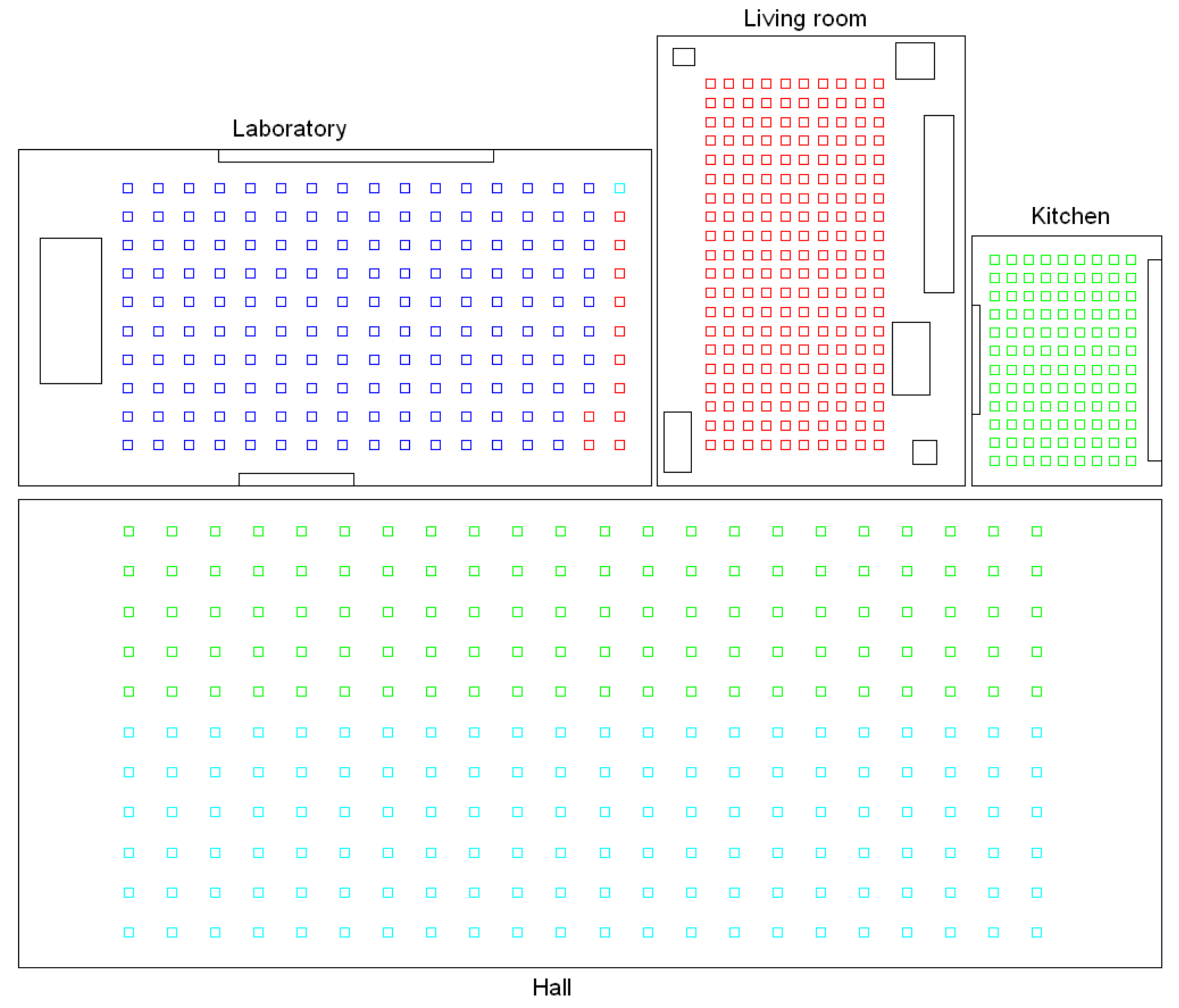
Figure 5.
Results of the intermediate-level clustering in the kitchen and laboratory, using the hierarchical algorithm and gist. Bielefeld dataset.
Figure 5.
Results of the intermediate-level clustering in the kitchen and laboratory, using the hierarchical algorithm and gist. Bielefeld dataset.

Figure 6.
Legend: ![Remotesensing 10 00522 i001]() Accuracy c;
Accuracy c; ![Remotesensing 10 00522 i002]() Correlation ;
Correlation ; ![Remotesensing 10 00522 i003]() Inconsistency . Results of the high-level clustering using the Fourier signature as global-appearance descriptor and (a) ; (b) ; and (c) . In the horizontal axes, to represent the distance measures.
Inconsistency . Results of the high-level clustering using the Fourier signature as global-appearance descriptor and (a) ; (b) ; and (c) . In the horizontal axes, to represent the distance measures.
 Accuracy c;
  Correlation ;
  Inconsistency . Results of the high-level clustering using the Fourier signature as global-appearance descriptor and (a) ; (b) ; and (c) . In the horizontal axes, to represent the distance measures.
Figure 6.
Legend: ![Remotesensing 10 00522 i001]() Accuracy c;
Accuracy c; ![Remotesensing 10 00522 i002]() Correlation ;
Correlation ; ![Remotesensing 10 00522 i003]() Inconsistency . Results of the high-level clustering using the Fourier signature as global-appearance descriptor and (a) ; (b) ; and (c) . In the horizontal axes, to represent the distance measures.
Inconsistency . Results of the high-level clustering using the Fourier signature as global-appearance descriptor and (a) ; (b) ; and (c) . In the horizontal axes, to represent the distance measures.
Accuracy c; Correlation ; Inconsistency . Results of the high-level clustering using the Fourier signature as global-appearance descriptor and (a) ; (b) ; and (c) . In the horizontal axes, to represent the distance measures.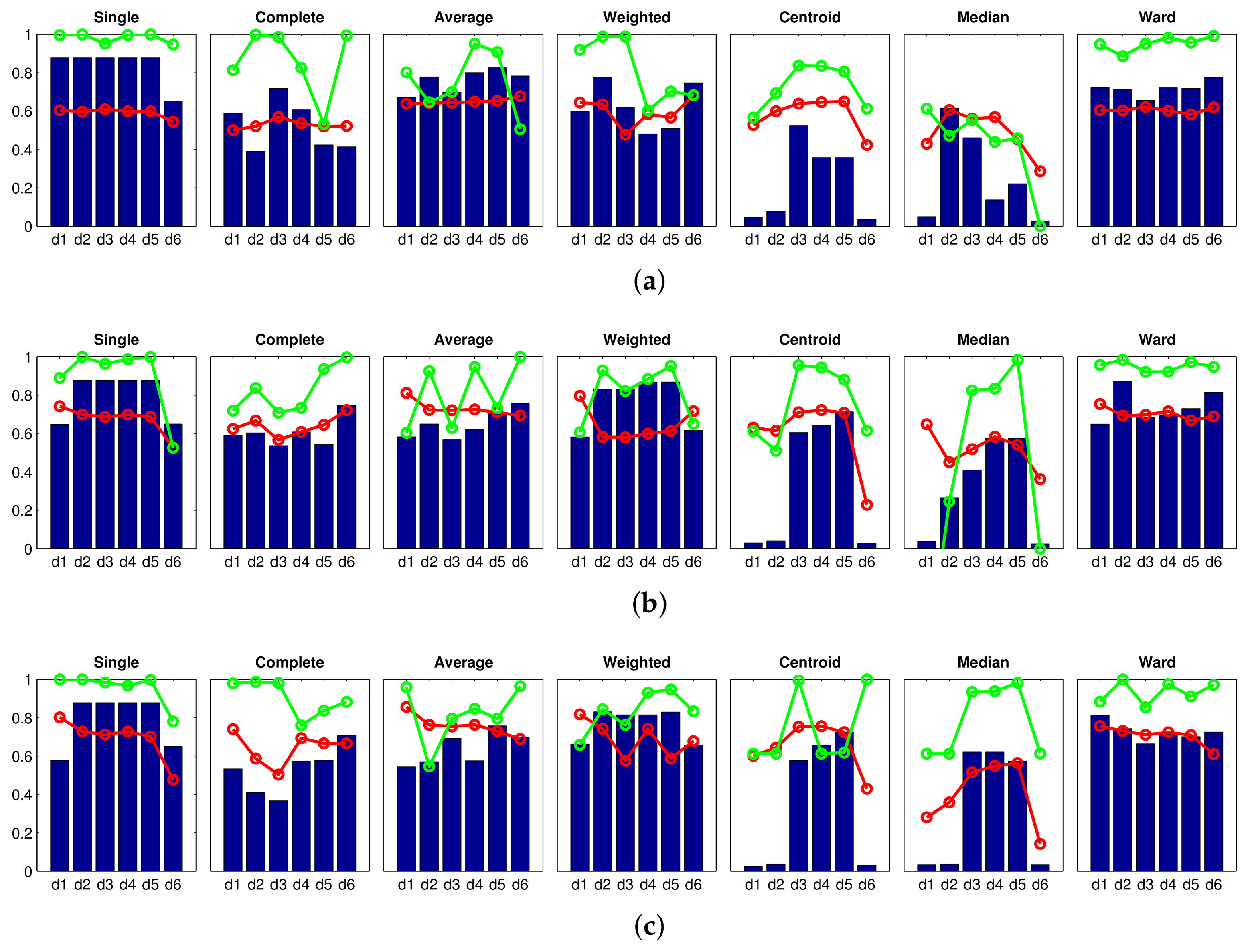
Figure 7.
Legend: ![Remotesensing 10 00522 i001]() Accuracy c;
Accuracy c; ![Remotesensing 10 00522 i002]() Correlation ;
Correlation ; ![Remotesensing 10 00522 i003]() Inconsistency . Results of the high-level clustering using rotational PCA as global-appearance descriptor, and (a) ; (b) ; and (c) .
Inconsistency . Results of the high-level clustering using rotational PCA as global-appearance descriptor, and (a) ; (b) ; and (c) .
Accuracy c; Correlation ; Inconsistency . Results of the high-level clustering using rotational PCA as global-appearance descriptor, and (a) ; (b) ; and (c) .
Figure 8.
Legend: ![Remotesensing 10 00522 i001]() Accuracy c;
Accuracy c; ![Remotesensing 10 00522 i002]() Correlation ;
Correlation ; ![Remotesensing 10 00522 i003]() Inconsistency . Results of the high-level clustering using HOG (Histogram of Oriented Gradients) as global-appearance descriptor and (a) ; (b) ; and (c) .
Inconsistency . Results of the high-level clustering using HOG (Histogram of Oriented Gradients) as global-appearance descriptor and (a) ; (b) ; and (c) .
Accuracy c; Correlation ; Inconsistency . Results of the high-level clustering using HOG (Histogram of Oriented Gradients) as global-appearance descriptor and (a) ; (b) ; and (c) .
Figure 9.
Legend: ![Remotesensing 10 00522 i001]() Accuracy c;
Accuracy c; ![Remotesensing 10 00522 i002]() Correlation ;
Correlation ; ![Remotesensing 10 00522 i003]() Inconsistency . Results of the high-level clustering using gist as global-appearance descriptor and (a) , ; (b) , ; (c) , .
Inconsistency . Results of the high-level clustering using gist as global-appearance descriptor and (a) , ; (b) , ; (c) , .
Accuracy c; Correlation ; Inconsistency . Results of the high-level clustering using gist as global-appearance descriptor and (a) , ; (b) , ; (c) , .
Figure 10.
Legend: ![Remotesensing 10 00522 i001]() Accuracy c;
Accuracy c; ![Remotesensing 10 00522 i002]() Correlation ;
Correlation ; ![Remotesensing 10 00522 i003]() Inconsistency . Results of the high-level clustering using gist as global-appearance descriptor and (a) , ; (b) , ; (c) , .
Inconsistency . Results of the high-level clustering using gist as global-appearance descriptor and (a) , ; (b) , ; (c) , .
Accuracy c; Correlation ; Inconsistency . Results of the high-level clustering using gist as global-appearance descriptor and (a) , ; (b) , ; (c) , .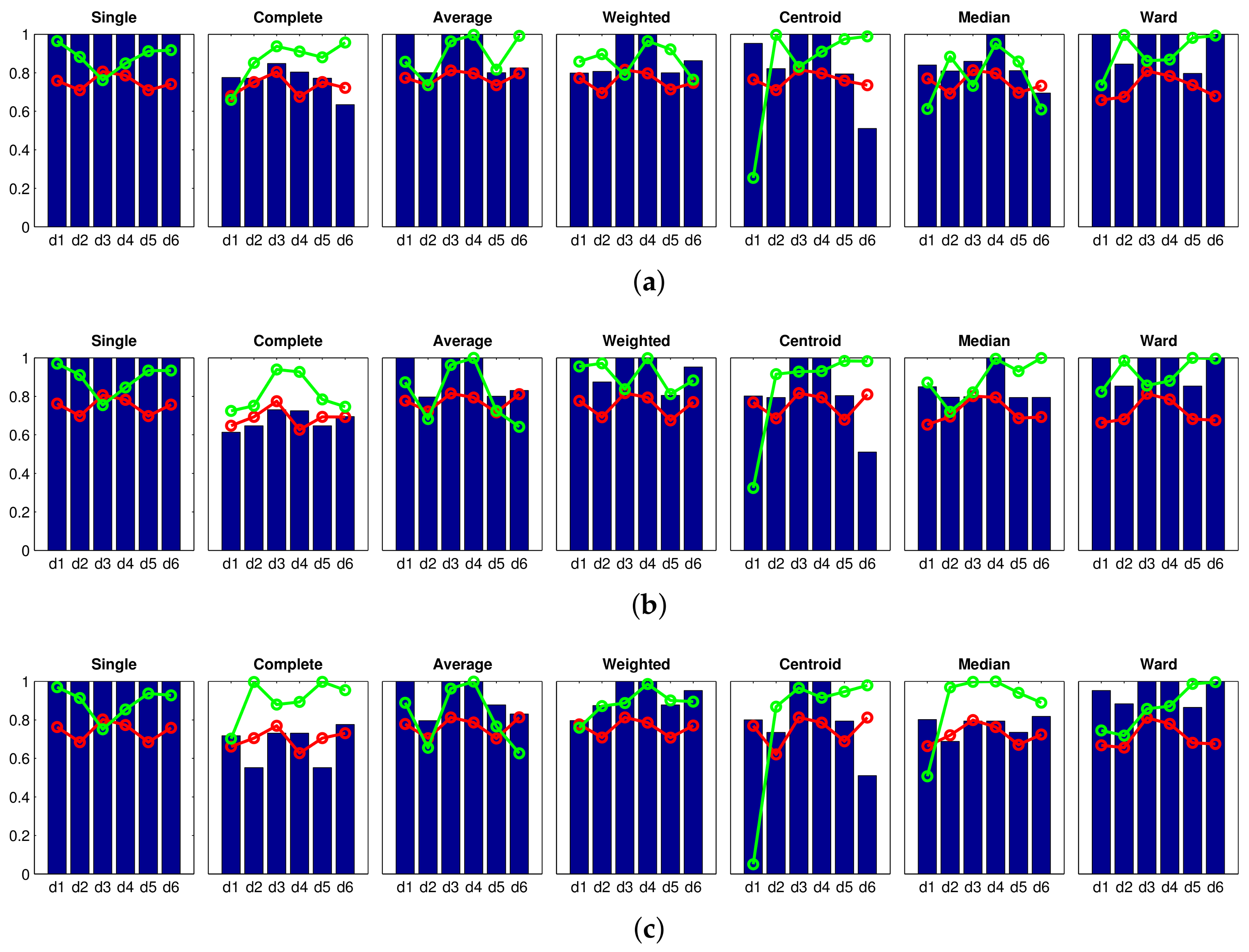
Figure 11.
Legend: ![Remotesensing 10 00522 i001]() Accuracy c;
Accuracy c; ![Remotesensing 10 00522 i002]() Correlation ;
Correlation ; ![Remotesensing 10 00522 i003]() Inconsistency . Results of the high-level clustering using CNN as global-appearance descriptor and (a) layer fc7 (4096 components); (b) layer fc8 (205 components).
Inconsistency . Results of the high-level clustering using CNN as global-appearance descriptor and (a) layer fc7 (4096 components); (b) layer fc8 (205 components).
Accuracy c; Correlation ; Inconsistency . Results of the high-level clustering using CNN as global-appearance descriptor and (a) layer fc7 (4096 components); (b) layer fc8 (205 components).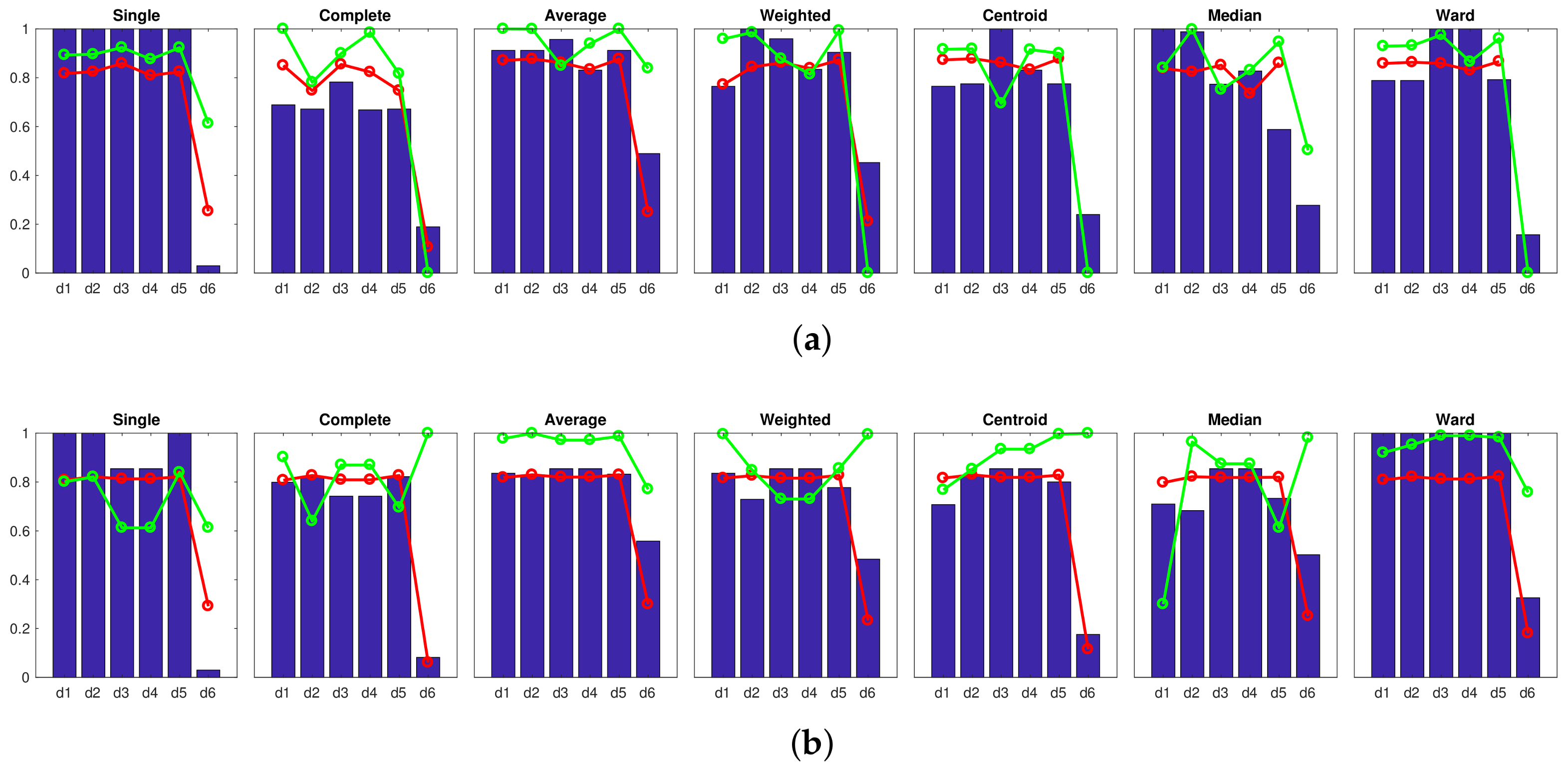
Figure 12.
Results of a sample unsuccessful clustering process performed with the images of the kitchen room. Bird’s eye view of the capture points, showing with colors their belonging to the resulting clusters, silhouette calculated from the visual descriptors and silhouette calculated from the coordinates of the capture points.

Figure 13.
Results of a sample successful clustering process performed with the images of the kitchen room. Bird’s eye view of the capture points, showing with colors their belonging to the resulting clusters, silhouette calculated from the visual descriptors and silhouette calculated from the coordinates of the capture points.
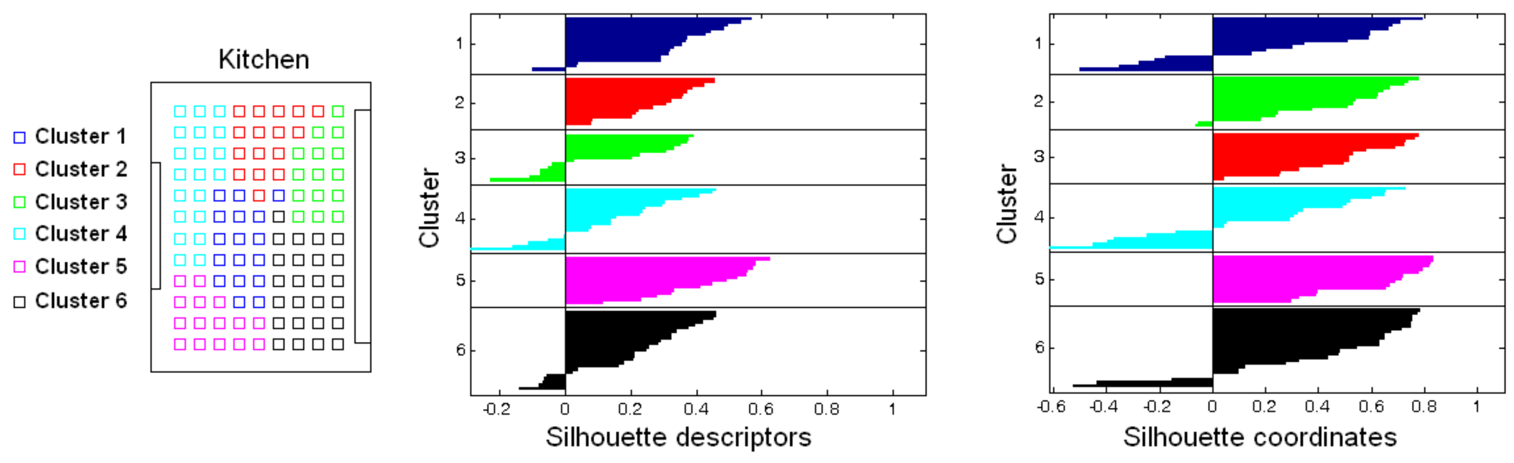
Figure 14.
Results of the intermediate-level mapping using gist with masks and horizontal blocks. Bird’s eye view of the four rooms of the Bielefeld set. The colors of the capture points indicate the cluster they belong to.
Figure 14.
Results of the intermediate-level mapping using gist with masks and horizontal blocks. Bird’s eye view of the four rooms of the Bielefeld set. The colors of the capture points indicate the cluster they belong to.
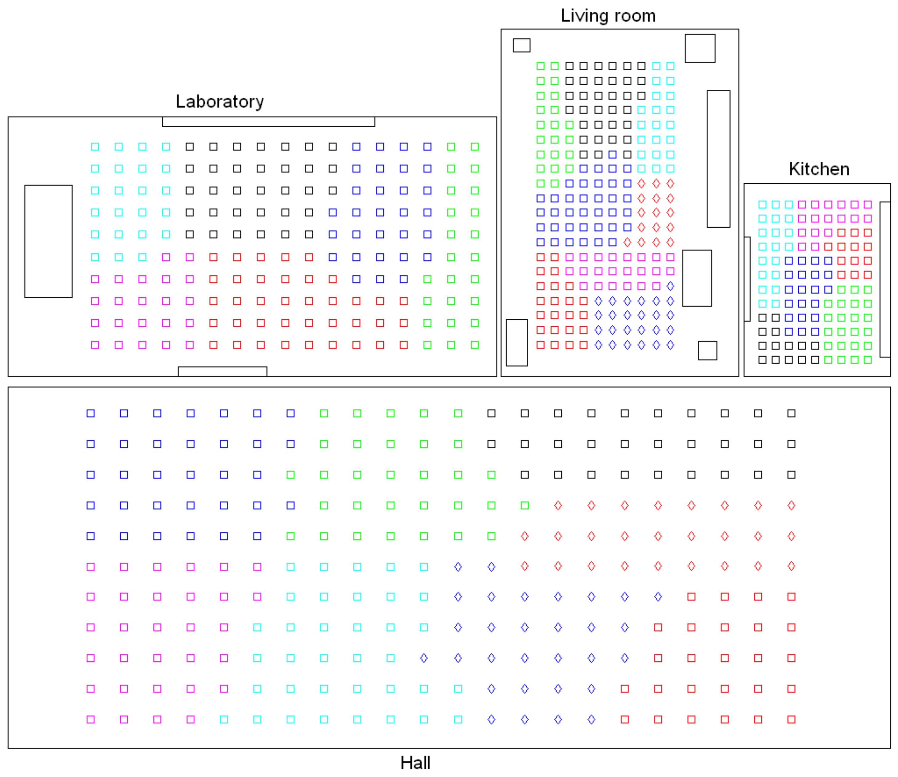
Figure 15.
Results of the intermediate-level mapping using gist with masks and horizontal blocks. Top row: silhouettes of the entities (visual descriptors). Bottom row: silhouettes of the coordinates of the capture points.
Figure 15.
Results of the intermediate-level mapping using gist with masks and horizontal blocks. Top row: silhouettes of the entities (visual descriptors). Bottom row: silhouettes of the coordinates of the capture points.
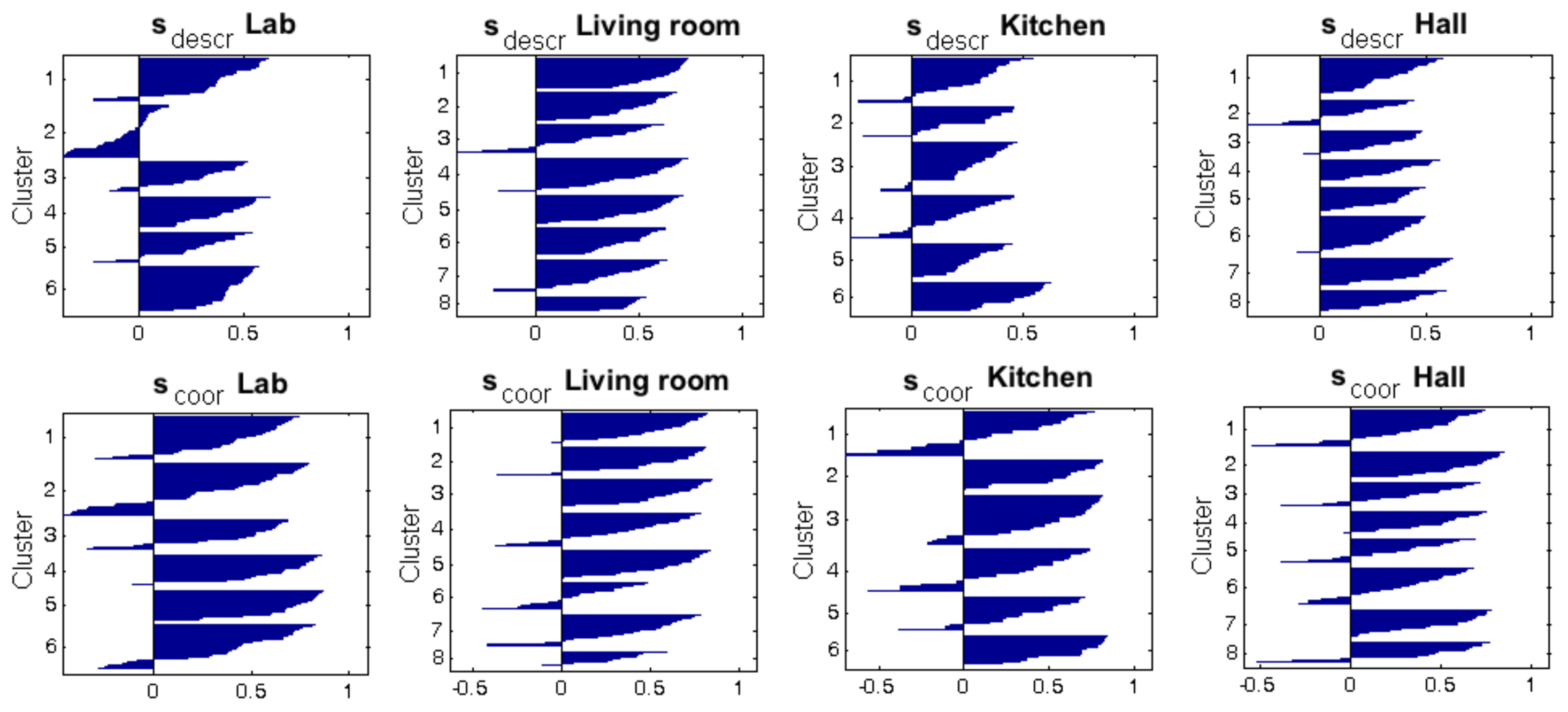
Figure 16.
Results of the intermediate-level mapping using HOG with horizontal cells. Bird’s eye view of the four rooms of the Bielefeld set. The colors of the capture points indicate the cluster they belong to.
Figure 16.
Results of the intermediate-level mapping using HOG with horizontal cells. Bird’s eye view of the four rooms of the Bielefeld set. The colors of the capture points indicate the cluster they belong to.
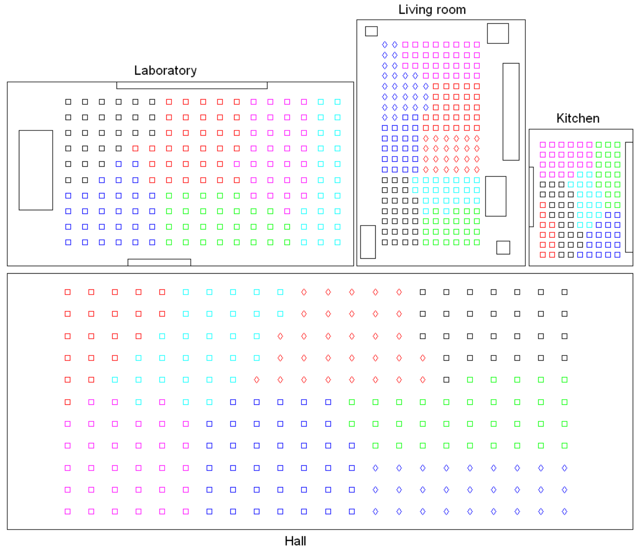
Figure 17.
Results of the intermediate-level mapping using Fourier signature with components per row. Bird’s eye view of the four rooms of the Bielefeld set. The colors of the capture points indicate the cluster they belong to.
Figure 17.
Results of the intermediate-level mapping using Fourier signature with components per row. Bird’s eye view of the four rooms of the Bielefeld set. The colors of the capture points indicate the cluster they belong to.
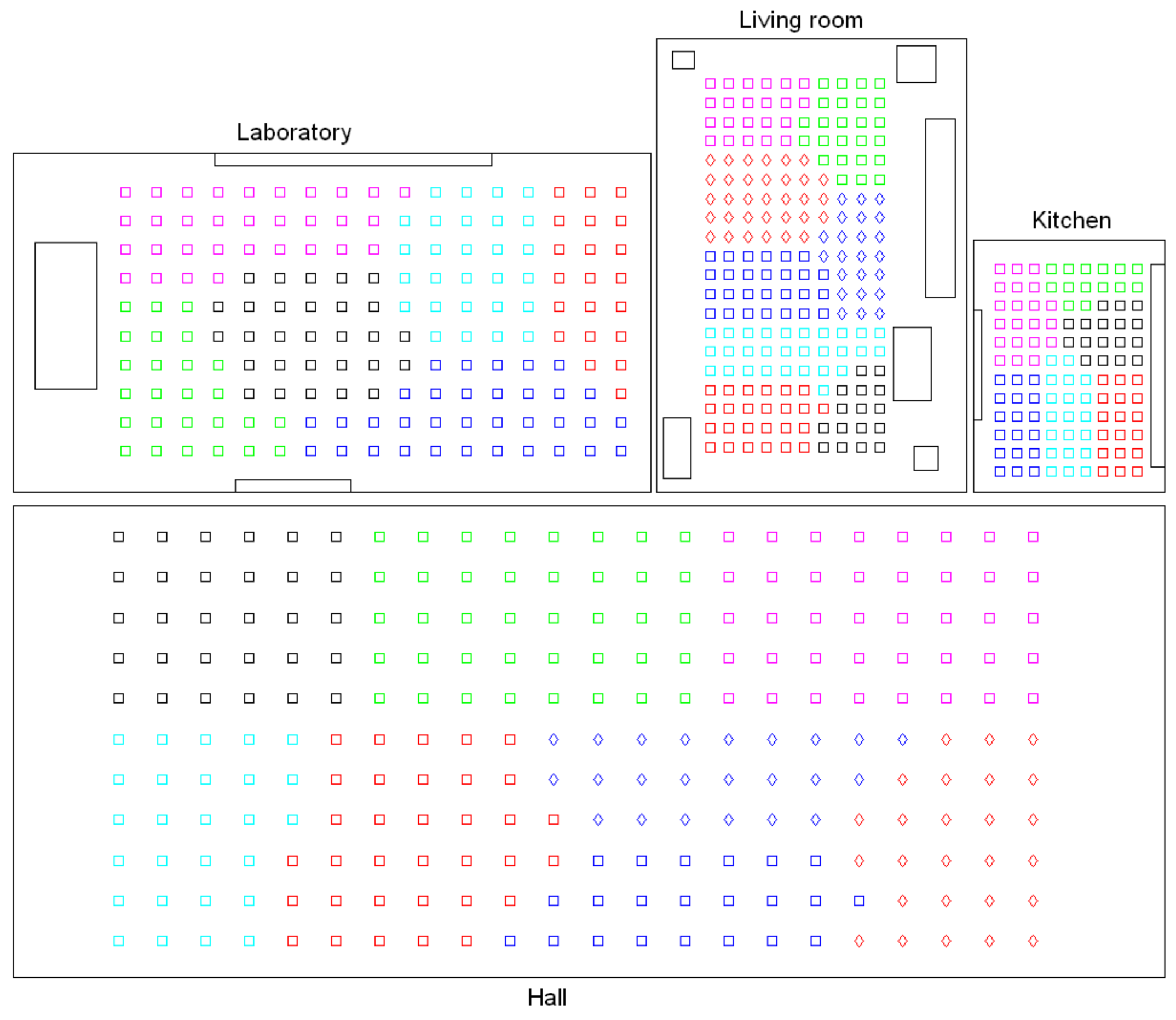
Figure 18.
Results of the intermediate-level mapping using CNN and the layer fc7 (4096 components). Bird’s eye view of the four rooms of the Bielefeld set. The colors of the capture points indicate the cluster they belong to.
Figure 18.
Results of the intermediate-level mapping using CNN and the layer fc7 (4096 components). Bird’s eye view of the four rooms of the Bielefeld set. The colors of the capture points indicate the cluster they belong to.

Figure 19.
Legend: ![Remotesensing 10 00522 i001]() Accuracy c;
Accuracy c; ![Remotesensing 10 00522 i002]() Correlation ;
Correlation ; ![Remotesensing 10 00522 i003]() Inconsistency . Results of the high-level clustering with the complete dataset. Gist descriptor (a) , ; (b) , ; (c) , .
Inconsistency . Results of the high-level clustering with the complete dataset. Gist descriptor (a) , ; (b) , ; (c) , .
Accuracy c; Correlation ; Inconsistency . Results of the high-level clustering with the complete dataset. Gist descriptor (a) , ; (b) , ; (c) , .
Figure 20.
Legend: ![Remotesensing 10 00522 i001]() Accuracy c;
Accuracy c; ![Remotesensing 10 00522 i002]() Correlation ;
Correlation ; ![Remotesensing 10 00522 i003]() Inconsistency . Results of the high-level clustering with the complete dataset. CNN descriptor (a) layer fc7 (4096 components) and (b) layer fc8 (205 components).
Inconsistency . Results of the high-level clustering with the complete dataset. CNN descriptor (a) layer fc7 (4096 components) and (b) layer fc8 (205 components).
Accuracy c; Correlation ; Inconsistency . Results of the high-level clustering with the complete dataset. CNN descriptor (a) layer fc7 (4096 components) and (b) layer fc8 (205 components).
Figure 21.
Results of the intermediate-level mapping using gist with masks and horizontal blocks. Bird’s eye view of the four additional rooms considered to validate the approach. The colors of the capture points indicate the cluster they belong to.
Figure 21.
Results of the intermediate-level mapping using gist with masks and horizontal blocks. Bird’s eye view of the four additional rooms considered to validate the approach. The colors of the capture points indicate the cluster they belong to.

Figure 22.
Sample panoramic images extracted from the database. (a,b) were captured from two distant positions of the hall, (c,d) were captured from two distant positions of the hall 2 and (e,f) were captured from two different poses of the events room.
Figure 22.
Sample panoramic images extracted from the database. (a,b) were captured from two distant positions of the hall, (c,d) were captured from two distant positions of the hall 2 and (e,f) were captured from two different poses of the events room.


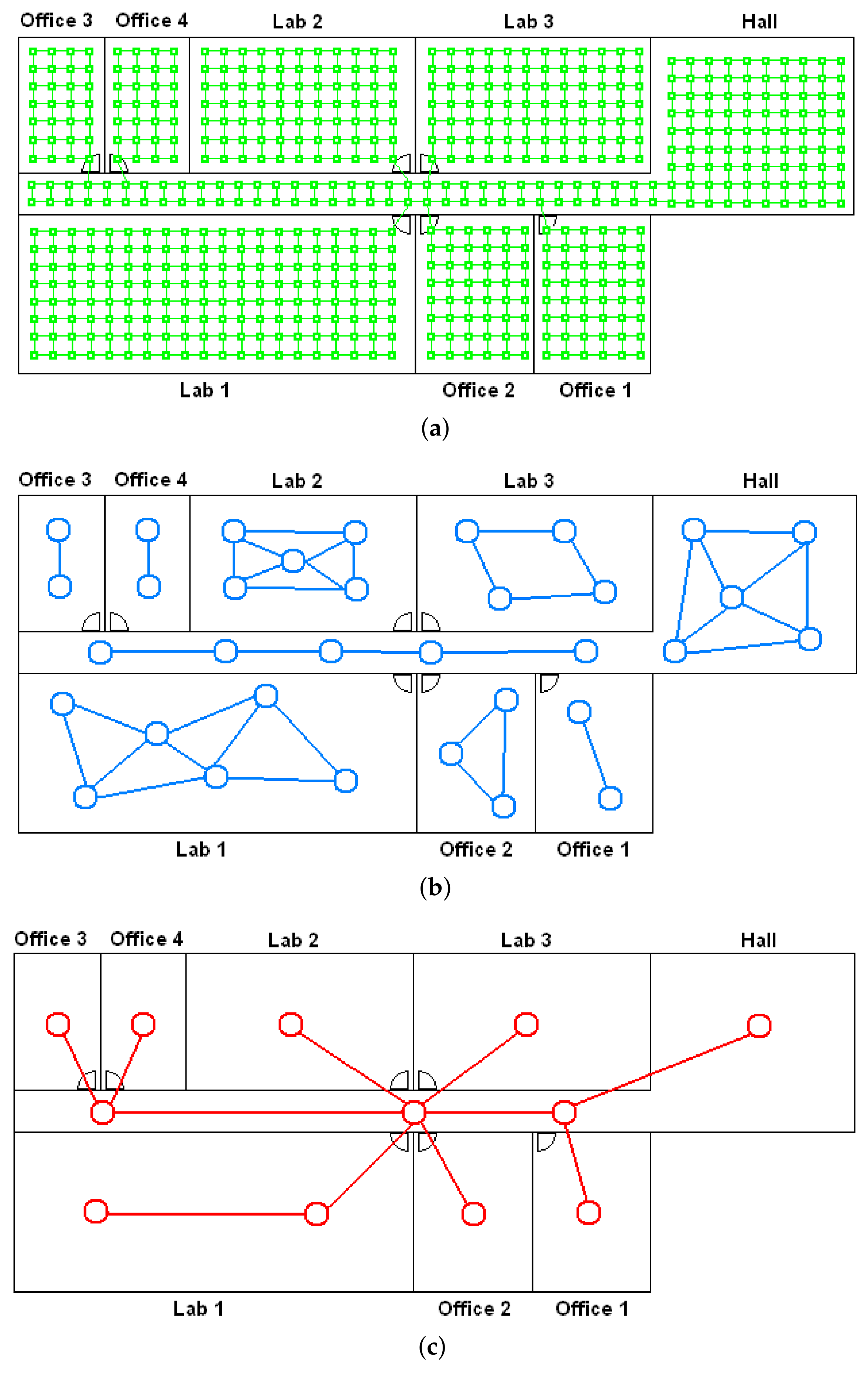
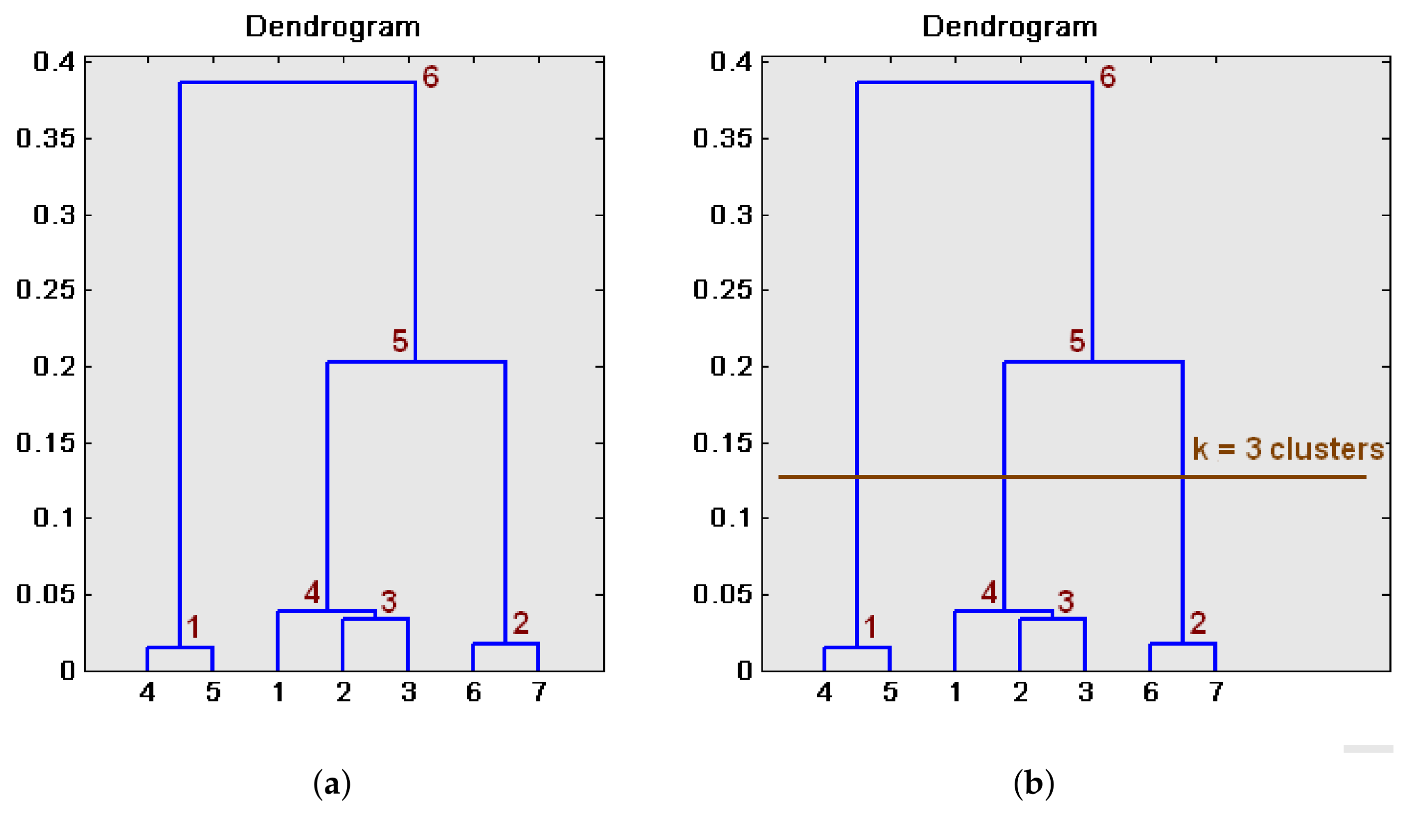
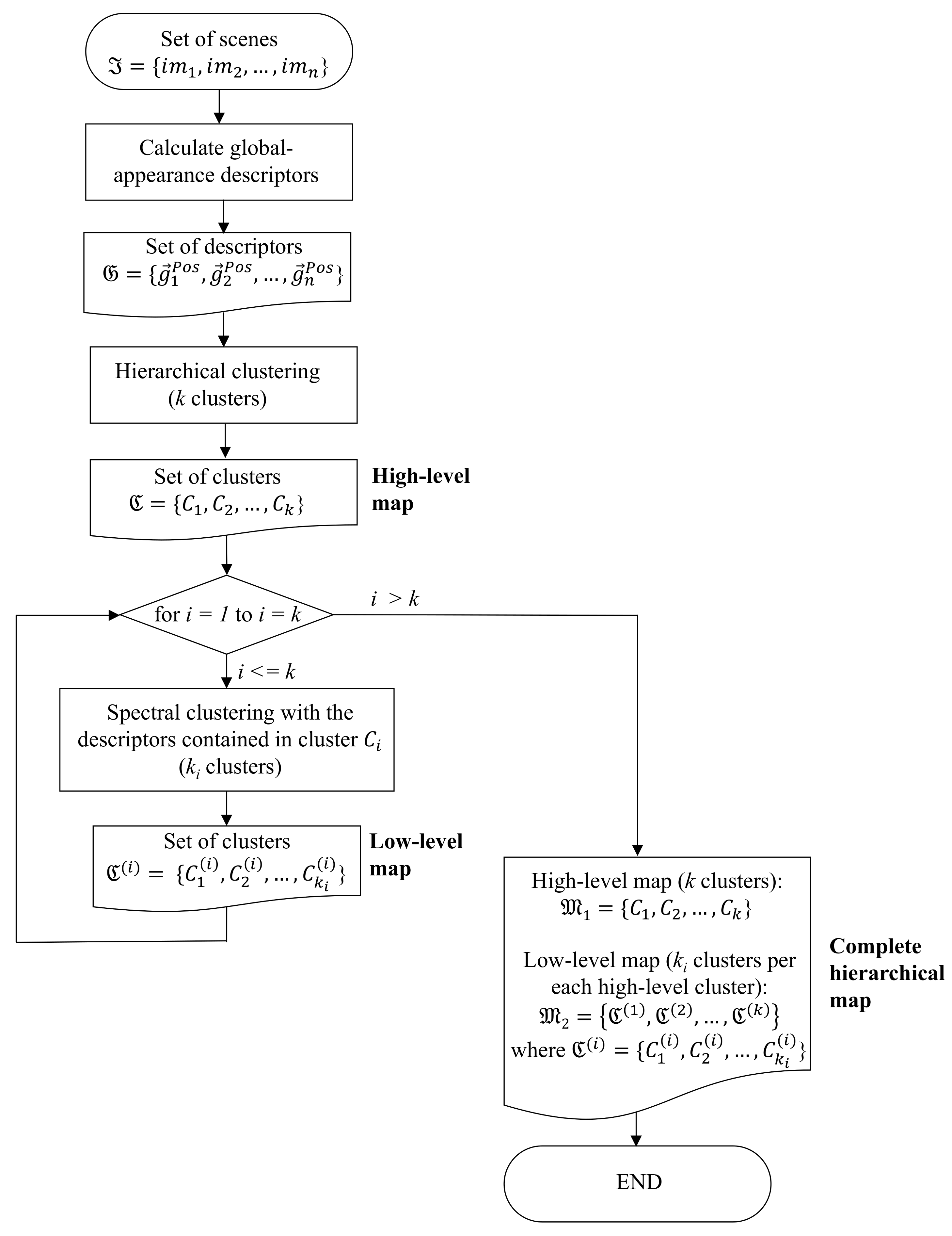
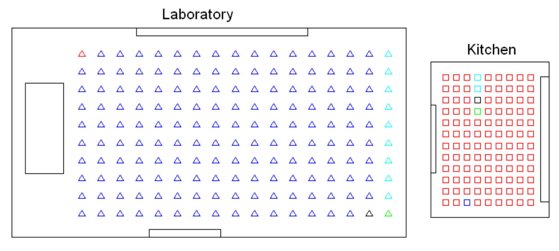
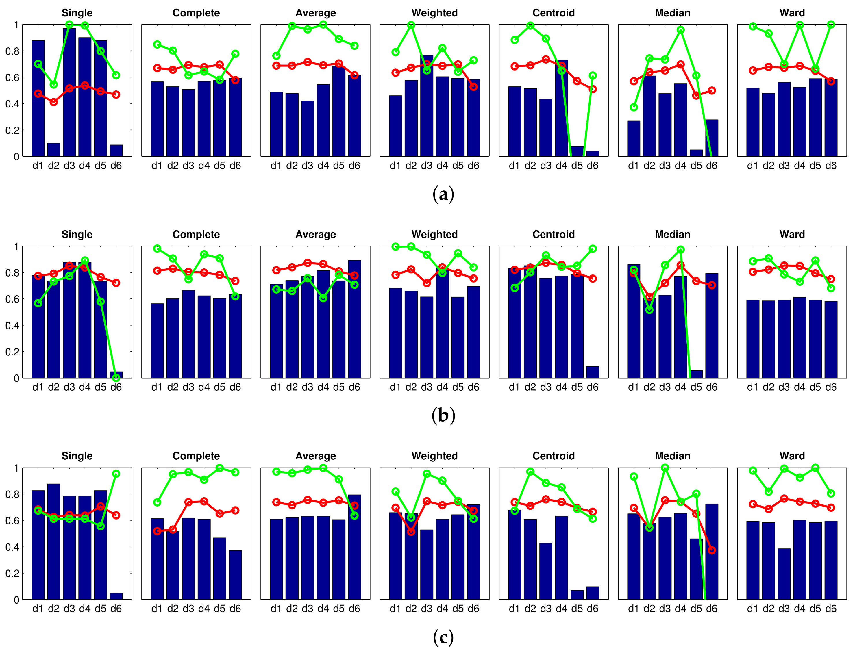
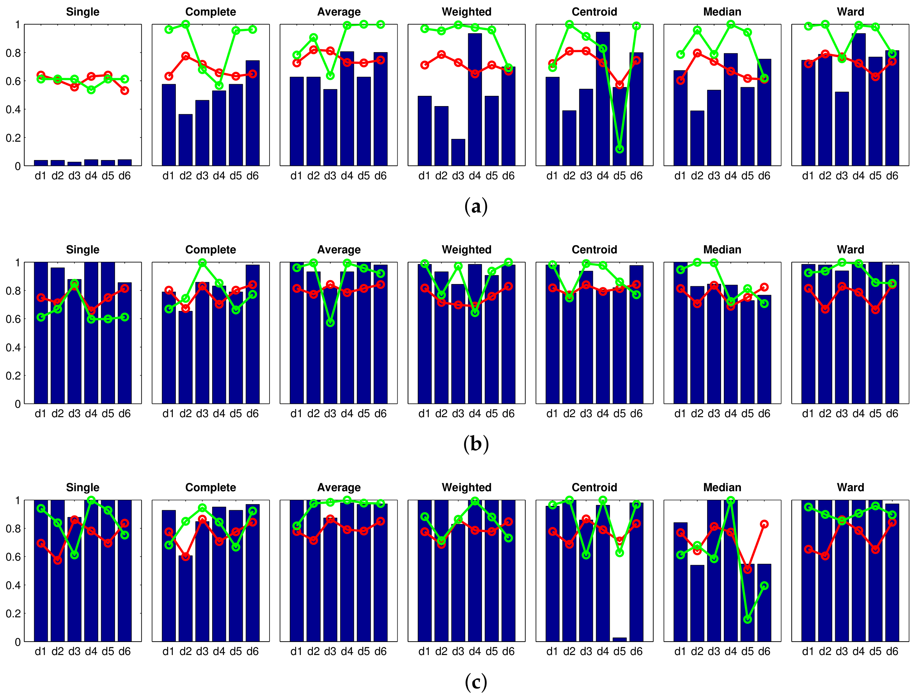
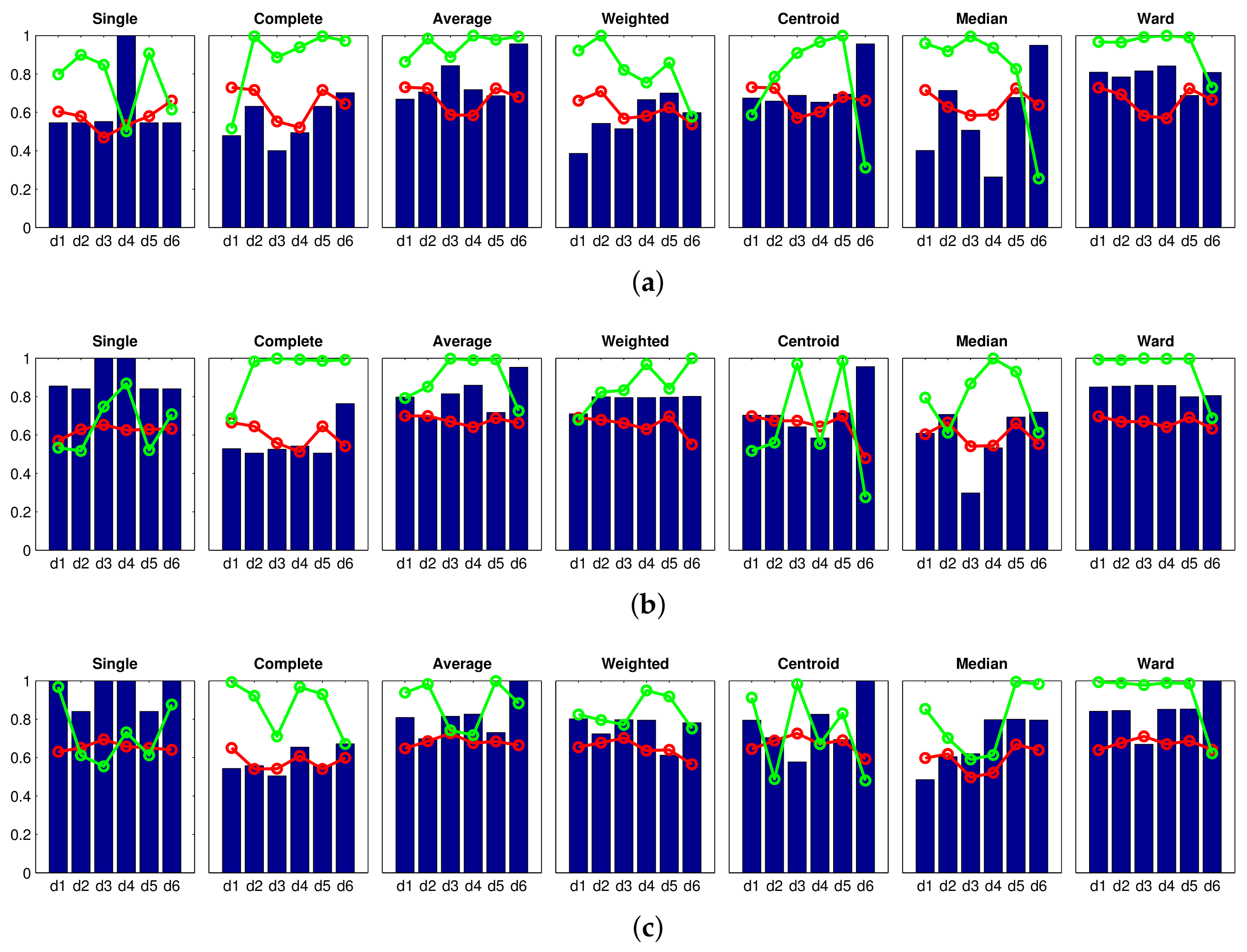
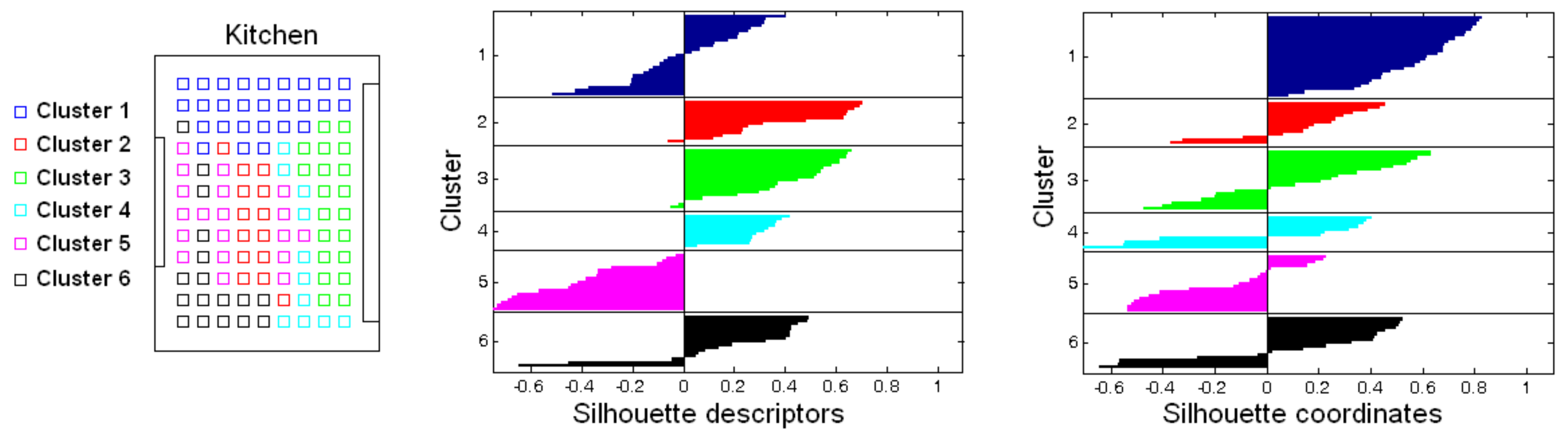
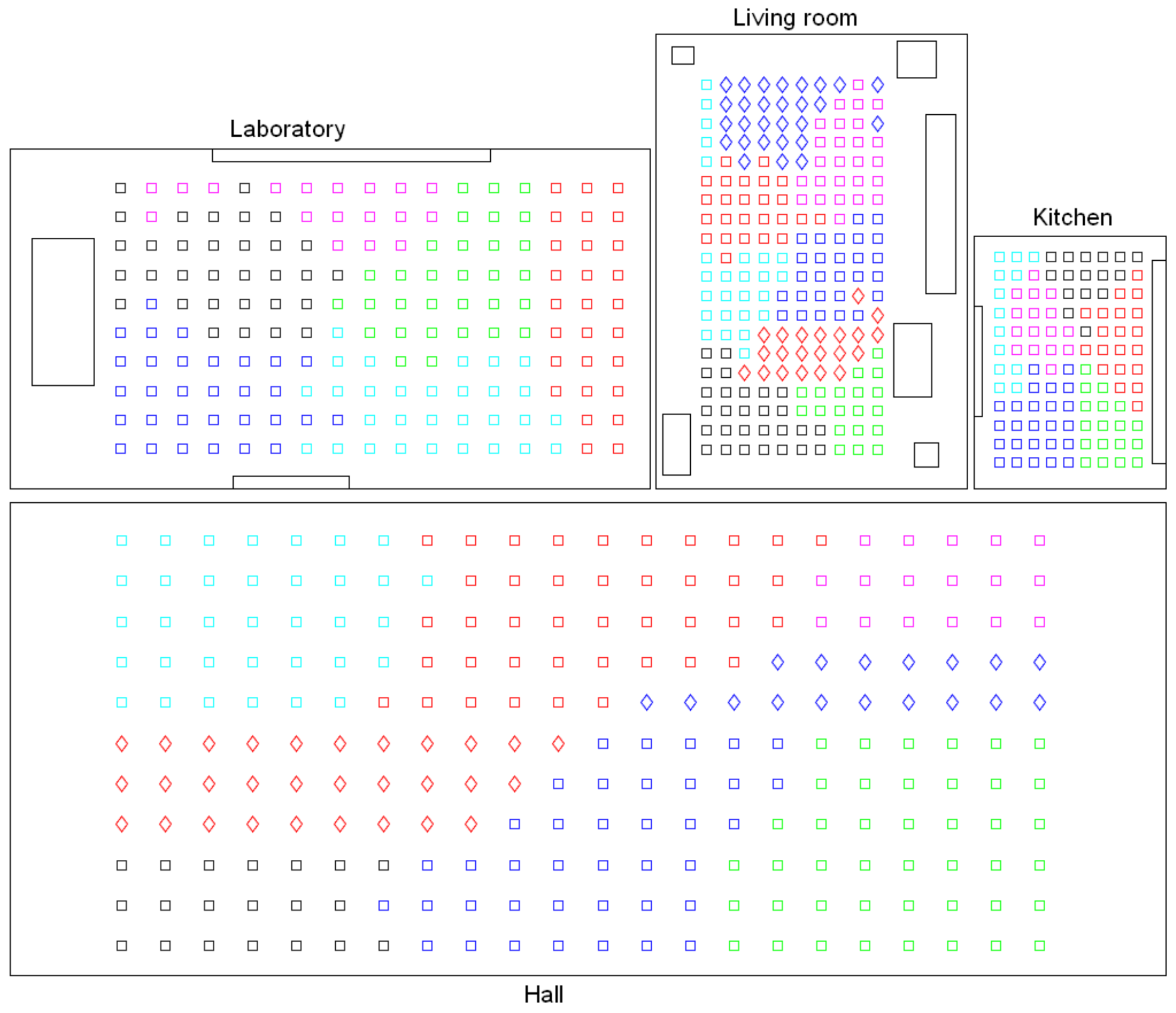
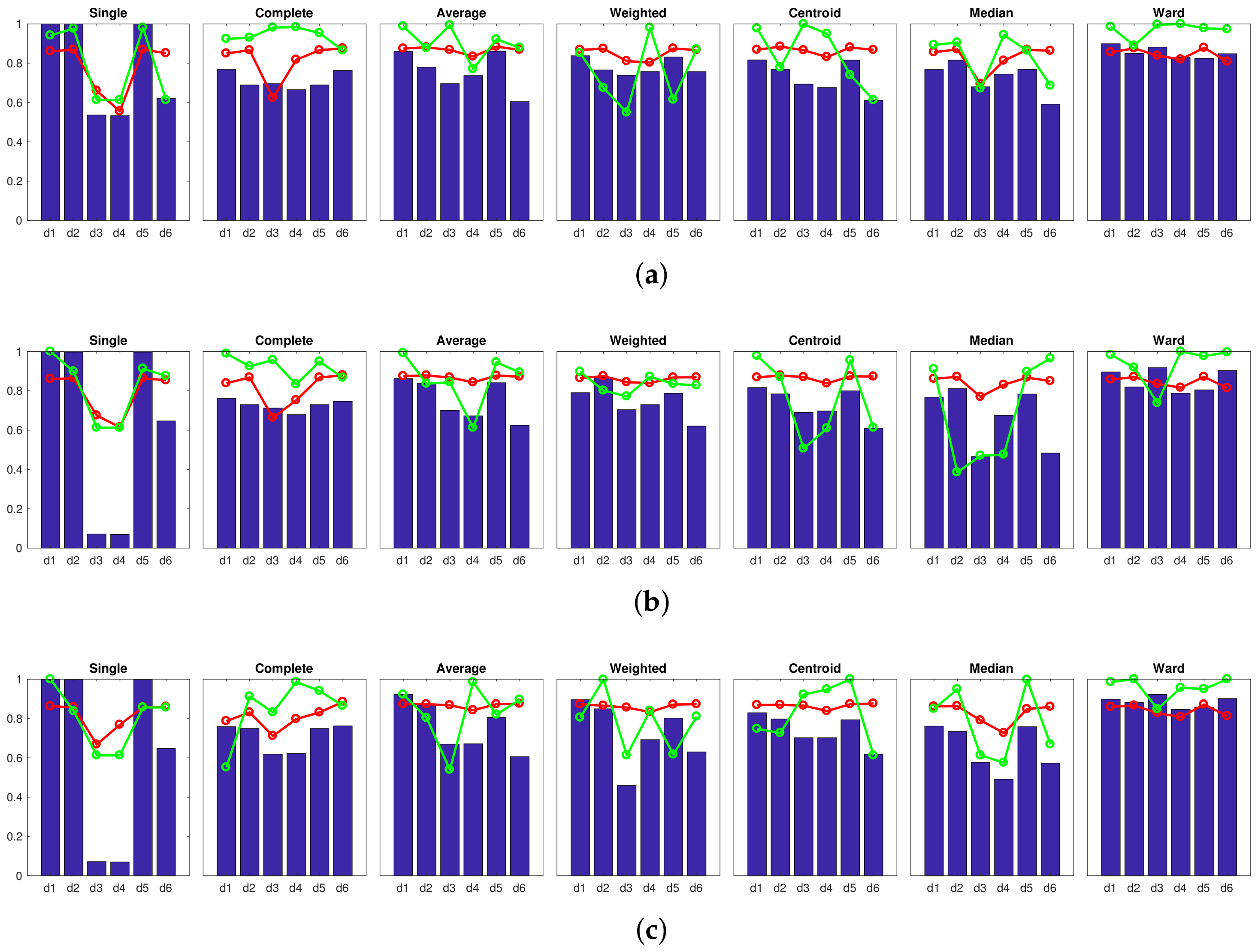
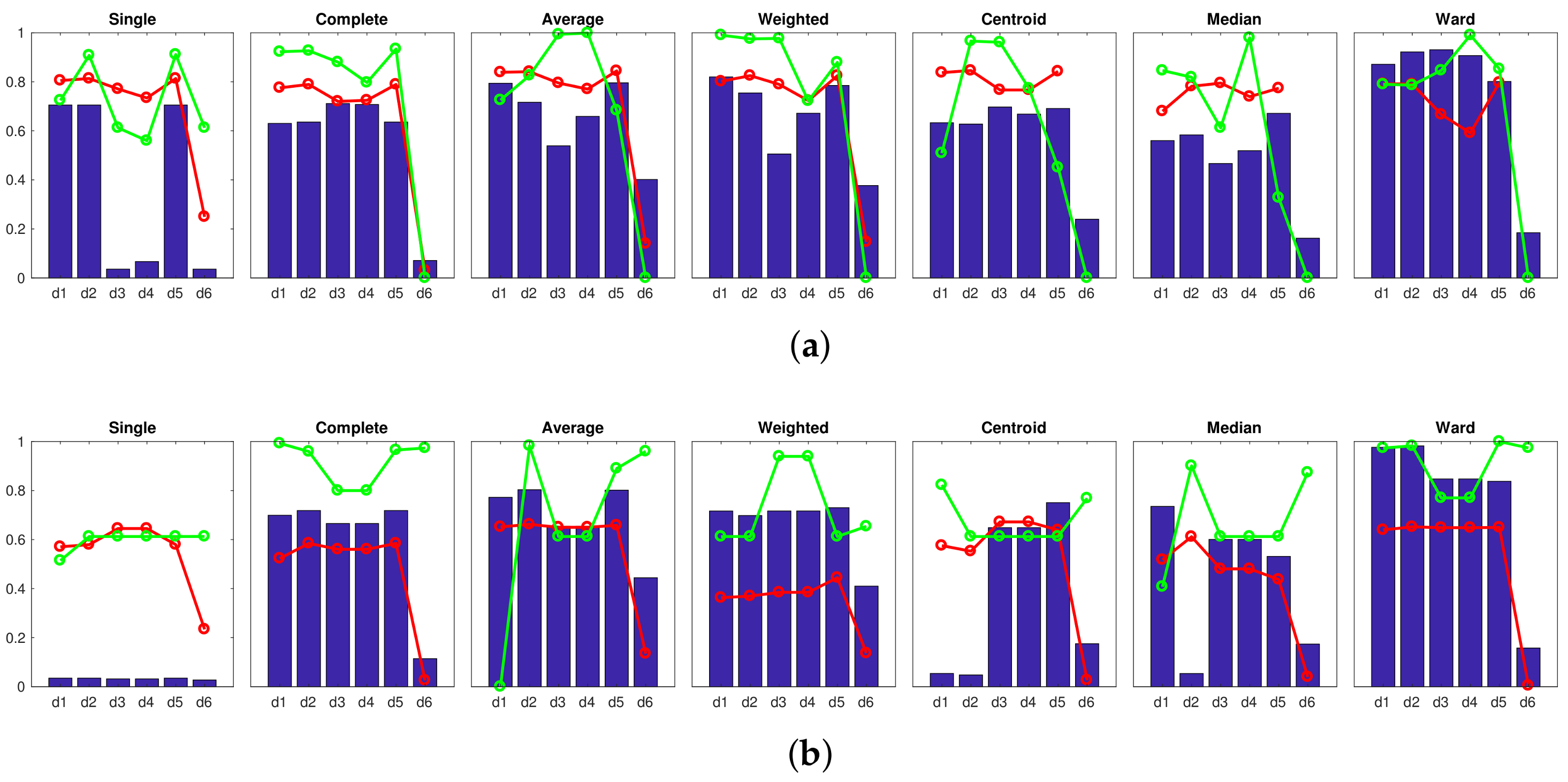
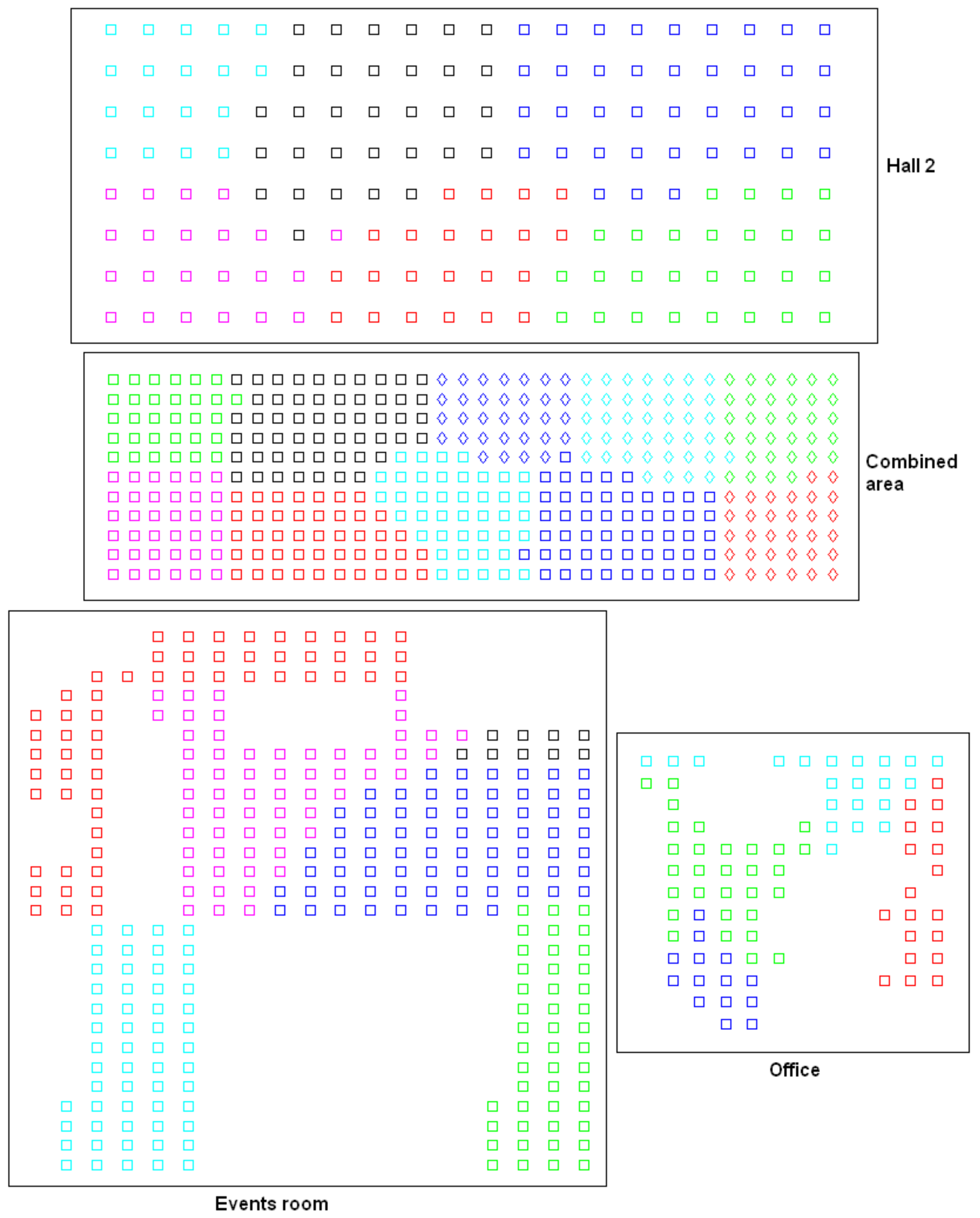
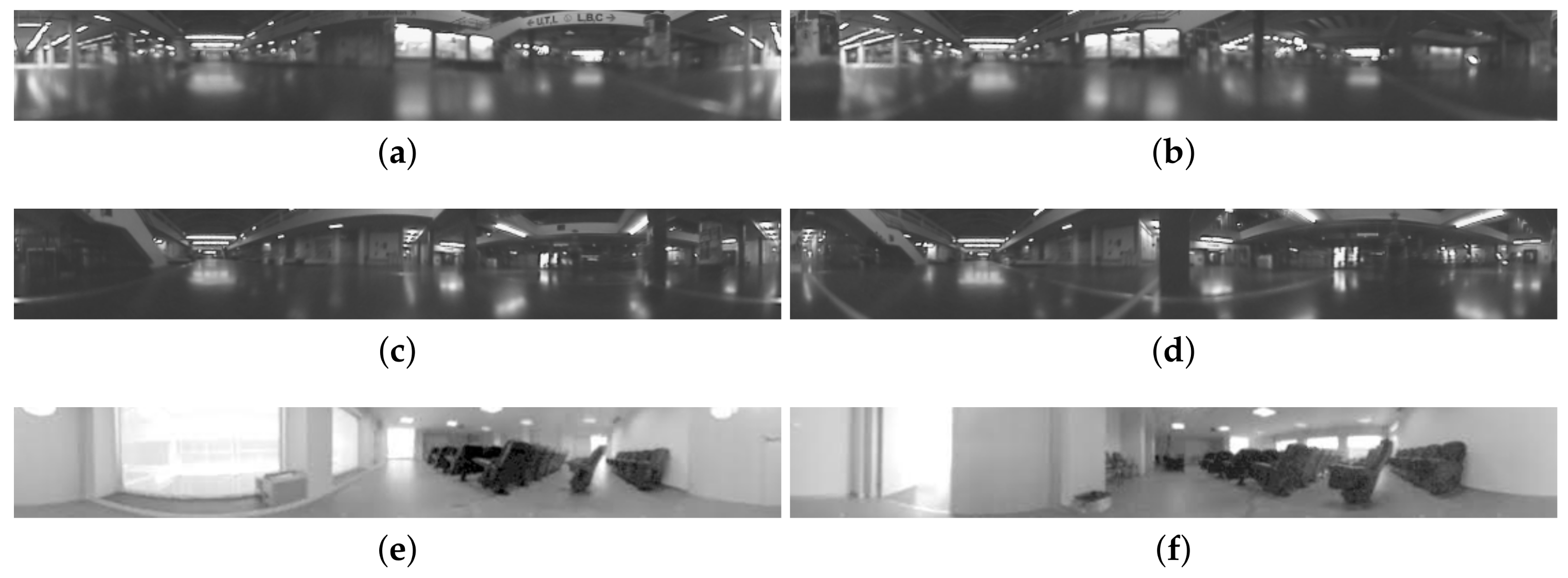
Table 1.
Methods to calculate the distance between two clusters in the hierarchical clustering process.
Table 1.
Methods to calculate the distance between two clusters in the hierarchical clustering process.
| Method | |
|---|---|
| Shortest distance (single) | where: |
| Longest distance (complete) | where: |
| Average unweighted distance (average) | |
| Average weighted distance (weighted) | The distance is obtained recursively: |
| Distance between unweighted centroids (centroid) | where: |
| Distance between weighted centroids (median) | where is built recursively |
| Minimum intracluster variance (Ward) |
Table 2.
Main features of the sets of images used to perform the experiments.
| Room Type | Number of Images | Grid Size (cm) | Room Size (m) | Resolution (pixels) |
|---|---|---|---|---|
| Laboratory | 170 | |||
| Hall | 200 | |||
| Kitchen | 108 | |||
| Living room | 242 | |||
| Total | 720 |
Table 3.
Optimal results of the high-level clustering for each description method.
| Descriptor and Configuration | Results | |||||
|---|---|---|---|---|---|---|
| Descriptor | Configuration | Method | Distance | Accuracy | ||
| Fourier sig. | Single | 0.8780 | 1.0000 | 0.7189 | ||
| Rot. PCA | Single | 0.9606 | 1.0000 | 0.5142 | ||
| HOG | Centroid | 1.0000 | 1.0000 | 0.6869 | ||
| Gist | Average | 1.0000 | 1.0000 | 0.7941 | ||
| CNN | Layer fc8 | Ward | 1.0000 | 0.9897 | 0.8188 | |
Table 4.
Results of the intermediate-clustering process. Average silhouette calculated from the descriptors (and standard deviation ) and from the coordinates of the capture points (and standard deviation ).
Table 4.
Results of the intermediate-clustering process. Average silhouette calculated from the descriptors (and standard deviation ) and from the coordinates of the capture points (and standard deviation ).
| Silhouette Descriptors | Silhouette Coordinates | ||||
|---|---|---|---|---|---|
| Descriptor | Configuration | ||||
| Fourier sig. | 0.2811 | 0.0021 | 0.3323 | 0.0276 | |
| 0.2160 | 0.0036 | 0.3284 | 0.0055 | ||
| 0.2211 | 0.0070 | 0.3662 | 0.0075 | ||
| 0.1990 | 0.0065 | 0.3666 | 0.0154 | ||
| 0.1833 | 0.0037 | 0.3379 | 0.0163 | ||
| 0.1870 | 0.0038 | 0.3521 | 0.0101 | ||
| Rot. PCA | 0.2532 | 0.0011 | 0.3962 | 0.0027 | |
| 0.2464 | 0.0032 | 0.2845 | 0.0083 | ||
| 0.1880 | 0.0076 | 0.2404 | 0.0268 | ||
| 0.1681 | 0.0118 | 0.1571 | 0.0167 | ||
| 0.1541 | 0.0091 | 0.2165 | 0.0193 | ||
| HOG | 0.1375 | 0.0034 | 0.1039 | 0.0089 | |
| 0.2893 | 0.0000 | 0.2564 | 0.0000 | ||
| 0.2886 | 0.0022 | 0.2880 | 0.0022 | ||
| 0.2114 | 0.0040 | 0.3000 | 0.0029 | ||
| 0.1630 | 0.0037 | 0.3217 | 0.0059 | ||
| Gist | 0.1363 | 0.0058 | -0.0537 | 0.0162 | |
| 0.1779 | 0.0090 | 0.1045 | 0.0165 | ||
| 0.2368 | 0.0070 | 0.2479 | 0.0190 | ||
| 0.2680 | 0.0152 | 0.1667 | 0.0106 | ||
| 0.2733 | 0.0000 | 0.1271 | 0.0000 | ||
| Gist | 0.2068 | 0.0168 | 0.2924 | 0.0397 | |
| 0.2262 | 0.0045 | 0.4277 | 0.0222 | ||
| 0.1878 | 0.0154 | 0.3103 | 0.0267 | ||
| 0.2071 | 0.0091 | 0.3921 | 0.0287 | ||
| 0.2125 | 0.0113 | 0.3887 | 0.0215 | ||
| Gist | 0.1707 | 0.0033 | 0.2894 | 0.0091 | |
| 0.1997 | 0.0149 | 0.3728 | 0.0403 | ||
| 0.2066 | 0.0162 | 0.3660 | 0.0415 | ||
| 0.1716 | 0.0179 | 0.2620 | 0.0464 | ||
| 0.1923 | 0.0093 | 0.2631 | 0.0375 | ||
| CNN | Layer fc7 | 0.2577 | 0.1082 | 0.3557 | 0.2075 |
| Layer fc8 | 0.2401 | 0.1196 | 0.3061 | 0.2382 | |
Table 5.
Main features of the additional sets of images used to perform the final tests.
| Room Type | Number of Images | Grid Size (cm) | Room Size (m) | Resolution (pixels) |
|---|---|---|---|---|
| Hall 2 | 160 | |||
| Combined area | 396 | |||
| Office | 84 | |||
| Events room | 300 | |||
| Total | 940 |
Table 6.
Results of the localization process using the gist descriptor. Comparative between hierarchical and global localization. Percentage of correct localizations and average time to obtain a result.
Table 6.
Results of the localization process using the gist descriptor. Comparative between hierarchical and global localization. Percentage of correct localizations and average time to obtain a result.
| Hierarchical Localization | Global Localization | ||||
|---|---|---|---|---|---|
| m | % correct | % correct | |||
| 4 | 4 | 80 | 0.47 | 82.5 | 0.59 |
| 8 | 87.5 | 0.51 | 90 | 0.82 | |
| 16 | 95 | 0.54 | 95 | 1.03 | |
| 32 | 97.5 | 0.60 | 97.5 | 1.52 | |
| 16 | 4 | 95 | 0.49 | 95 | 0.95 |
| 8 | 95 | 0.57 | 95 | 2.18 | |
| 16 | 100 | 0.80 | 100 | 5.18 | |
| 32 | 100 | 1.10 | 100 | 11.29 | |
| 32 | 4 | 95 | 0.54 | 95 | 1.41 |
| 8 | 97.5 | 0.82 | 97.5 | 5.20 | |
| 16 | 97.5 | 1.14 | 97.5 | 11.34 | |
| 32 | 100 | 1.64 | 100 | 22.54 | |
© 2018 by the authors. Licensee MDPI, Basel, Switzerland. This article is an open access article distributed under the terms and conditions of the Creative Commons Attribution (CC BY) license (http://creativecommons.org/licenses/by/4.0/).
Share and Cite
MDPI and ACS Style
Payá, L.; Peidró, A.; Amorós, F.; Valiente, D.; Reinoso, O. Modeling Environments Hierarchically with Omnidirectional Imaging and Global-Appearance Descriptors. Remote Sens. 2018, 10, 522. https://doi.org/10.3390/rs10040522
AMA Style
Payá L, Peidró A, Amorós F, Valiente D, Reinoso O. Modeling Environments Hierarchically with Omnidirectional Imaging and Global-Appearance Descriptors. Remote Sensing. 2018; 10(4):522. https://doi.org/10.3390/rs10040522
Chicago/Turabian StylePayá, Luis, Adrián Peidró, Francisco Amorós, David Valiente, and Oscar Reinoso. 2018. "Modeling Environments Hierarchically with Omnidirectional Imaging and Global-Appearance Descriptors" Remote Sensing 10, no. 4: 522. https://doi.org/10.3390/rs10040522
Note that from the first issue of 2016, this journal uses article numbers instead of page numbers. See further details here.