Assessment of Methods for Passive Microwave Snow Cover Mapping Using FY-3C/MWRI Data in China


1
State Key Laboratory of Remote Sensing Science, Jointly Sponsored by Beijing Normal University and Institute of Remote Sensing and Digital Earth of Chinese Academy of Sciences, Faculty of Geographical Science, Beijing Normal University and Joint Center for Global Change Studies, Beijing 100875, China
2
National Satellite Meteorological Center, China Meteorological Administration, Beijing 100081, China
*
Author to whom correspondence should be addressed.
Remote Sens. 2018, 10(4), 524; https://doi.org/10.3390/rs10040524
Submission received: 10 January 2018
/
Revised: 27 February 2018
/
Accepted: 23 March 2018
/
Published: 27 March 2018
(This article belongs to the Special Issue Advances in Quantitative Remote Sensing in China – In Memory of Prof. Xiaowen Li)
Abstract
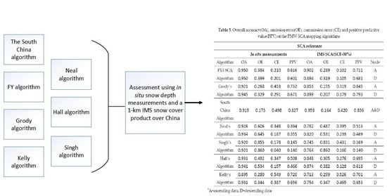
:Ongoing information on snow and its extent is critical for understanding global water and energy cycles. Passive microwave data have been widely used in snow cover mapping given their long-time observation capabilities under all-weather conditions. However, assessments of different passive microwave (PMW) snow cover area (SCA) mapping algorithms have rarely been reported, especially in China. In this study, the performances of seven PMW SCA mapping algorithms were tested using in situ snow depth measurements and a one-kilometer Interactive Multisensor Snow and Ice Mapping System (IMS) snow cover product over China. The selected algorithms are the FY3 algorithm, Grody’s algorithm, the South China algorithm, Kelly’s algorithm, Singh’s algorithm, Hall’s algorithm and Neal’s algorithm. During the test period, most algorithms performed reasonably well. The overall accuracy of all algorithms is higher than 0.895 against in situ observations and higher than 0.713 against the IMS product. In general, Singh’s algorithm, Hall’s algorithm and Neal’s algorithm had poor performance during the test. Their misclassification errors were larger than those of the remaining algorithms. Grody’s algorithm, the South China algorithm and Kelly’s algorithm had higher positive predictive values and lower omission errors than those of the others. The errors of these three algorithms were mainly caused by variations in commission errors. Comparing to Grody’s algorithm, the South China algorithm and Kelly’s algorithm, the FY3 algorithm presented a conservative snow cover estimation to balance the problem between snow identification and overestimation. As a result, the overall accuracy of the FY3 algorithm was the highest of all the tested algorithms. The accuracy of all algorithms tended to decline with a decreased snow cover fraction as well as SD < 5 cm. All tested algorithms have severe omission errors over barren land and grasslands. The results shown in this study contribute to ongoing efforts to improve the performance and applicability of PMW SCA algorithms.
1. Introduction
Snow cover is an important geophysical parameter for understanding global climate change, the radiation budget and the water cycle [1,2]. Given the importance of snow, snow cover extent has been a key observation target since the beginning of the satellite remote-sensing era dating to the mid-1960s [3]. Snow cover area (SCA) monitoring using optical and microwave sensors has been reported for decades [4]. A number of snow cover detection algorithms using optical sensors have been developed since the 1980s [5,6,7,8,9]. However, snow cover maps derived from optical sensors are strongly influenced by observation conditions such as cloud obscuration and solar illumination. Inaccessibility in cloud cover and weak sun exposure regions greatly limit the applicability of optical SCA products in regional and global applications [4].
Passive microwave (PMW) observation is another data source for SCA detection [10,11,12]. Dry snow is a type of microwave scattering material and can be identified by its volume scattering signature. The positive brightness temperature (Tb) gradient between low and high frequencies is a crucial criterion for snow cover identification [13]. Most PMW SCA detection algorithms are based on a decision tree classification approach. Snow can be distinguished from other scattering or non-scattering surfaces via various filters. These algorithms can be divided into three groups: (1) identify snow with detailed types of snow [14,15]; (2) identify snow and non-snow types simultaneously [16,17]; and (3) simply identify snow without any in-depth information [18,19,20].
The primary advantage of using PMW data is the ability of microwaves to observe land surface conditions through clouds during day and night. At present, the PMW SCA products have been mainly used to fill the cloud gap of long-term optical SCA products [21,22,23,24] or act as a preprocessing step for producing PMW snow water equivalent (SWE) and snow depth (SD) products [25,26,27,28]. Errors inherent to PMW SCA products propagate into and corrupt the combined products. The false snow and snow-free identifications affect the accuracy of the associated SD, SWE and SCA products. Thus, an in-depth evaluation is needed to understand the uncertainty of PMW SCA mapping methods as well as to develop new methods.
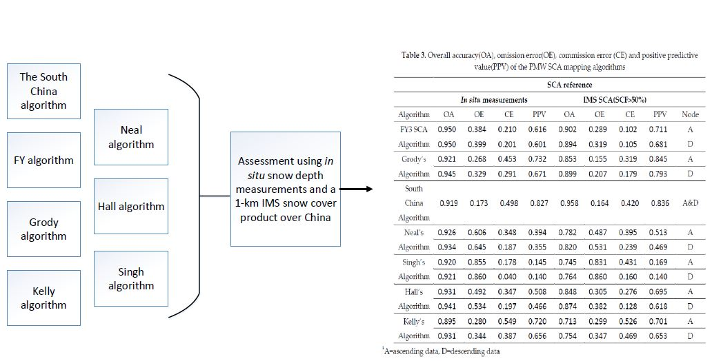
In this study, seven PMW SCA mapping methods were tested, including Kelly’s algorithm [14], the FY3 algorithm [15], Grody’s algorithm [16], the South China algorithm [17], Singh’s algorithm [18], and Hall’s algorithm [19], Neal’s algorithm [20]. These algorithms were selected because they are well-documented, have been successfully applied and have an indicative effect on later research. Common approaches for evaluating satellite-derived SCA would be to compare it to in situ measurements [11,29,30] or satellite images with higher spatial resolutions [8,31,32,33,34]. We used similar strategies in this assessment. The performance of different PMW SCA mapping algorithms was evaluated against in situ snow depth measurements along with the Multisensor Snow and Ice Mapping System (IMS) snow cover product at a one-kilometer resolution. The one-kilometer IMS snow cover product was taken as a validation dataset because it is cloud-free and of high spatial resolution (compared to PMW observations) and is a high-quality SCA product.
This paper is organized as follows. Section 2 describes the data used and the PMW SCA algorithms. Section 3 presents the evaluation results and the effects of land cover, snow cover fraction (SCF), and snow depth on SCA mapping accuracy. Section 4 is dedicated to the discussion of the tested algorithms. Finally, a conclusion has been presented in Section 5 for the whole work of this paper.
2. Data and Methodology
In this study, FY3C-MWRI data were used for snow cover mapping. In situ snow depth observations together with the IMS snow cover product were used to evaluate different PMW SCA mapping algorithms. The data and algorithms are described in detail in the following subsections.
2.1. FY-3C/MWRI Data
The FY-3C satellite is one of the second generation polar-orbit meteorological satellite series of China. The FY-3C satellite was launched on 23 September 2013 with the goal of observing global atmospheric and geophysical features around the clock. The Microwave Radiation Imager (MWRI) is one of the 13 remote-sensing instruments onboard the FY-3C satellite. MWRI is a ten-channel, five-frequency, PMW radiometer system. It measures horizontally and vertically polarized brightness temperatures ranging from 10.65 GHz to 89 GHz. The local time on the descending node (LTDN) is near 10:00 a.m. Spatial resolution of the individual measurements varies from 7.5 km × 12 km at 89 GHz to 51 km × 85 km at 10.65 GHz. The FY3C-MWRI L1 swath data are available from the China Meteorological Administration/National Satellite Meteorological Center website (http://www.nsmc.org.cn/).
2.2. In Situ Measurements
Daily meteorological data are provided by the National Meteorological Information Center, China Meteorological Administration. Daily SD observations from 753 stations (Figure 1) were used to evaluate the PMW snow cover detection algorithms during the snow season. Recorded variables of weather stations include site name, observation time, site location (latitude and longitude in degrees), geodetic elevation (m), surface temperature and snow depth (cm). The records were selected only if the surface temperature was less than 0 °C to avoid the impact of wet snow.
2.3. IMS Data
The IMS snow cover product of the National Ice Center combines multiple data sources to map daily cloud-free snow extent of the Northern Hemisphere at three different resolutions: 1 km, 4 km and 24 km. The 1-km IMS data became available during December of 2014. In this study, 1-km IMS data were used as the validation dataset. The data were obtained from the National Snow and Ice Data Center (http://nsidc.org/).
2.4. PMW Snow Cover Mapping Algorithms
Dry snow is a type of strong scattering material. Snow cover produces a positive brightness temperature gradient between low- and high-frequency channels [13]. Although this characteristic of scattering materials identifies snow, it identifies other scattering materials such as precipitation, deserts, and frozen ground [10] because these non-snow types may produce a spectral response in the microwave similar to that of snow. To objectively detect snow cover, various filters are used to separate scattering signals of snow cover from other scattering and non-scattering surfaces [35].
Seven PMW SCA mapping algorithms were selected for evaluation in this paper. Classification criteria of these algorithms are shown in Table 1. The frequencies listed in Table 1 are subject to FY-3C/MWRI. Grody’s algorithm and the South China algorithm identify snow and the non-snow types (precipitation, cold deserts and frozen soil) simultaneously. The FY3 algorithm and Kelly’s algorithm not only identify snow-covered areas but also divide snow into detailed categories. The last three algorithms are simply designed to detect snow.
3. Results and Analysis
To test and compare the performance of the seven algorithms, the SCAs derived from PMW SCA mapping algorithms were quantitatively evaluated using in situ SD observations and the one-kilometer IMS snow cover product. Only dry snow records of in situ observations were used for analysis because the seven tested algorithms are mostly for dry snow discrimination. The one-kilometer IMS data were reprojected to the projection of the PMW SCA maps. Then, the snow cover fraction in each PMW pixel was calculated. We set the threshold of a snow cover fraction value to 50% to determine whether pixels have snow or do not. All pixels with SCF less than the threshold were labelled snow-free.
Four assessment indexes, overall accuracy (OA), omission error (OE), commission error (CE), and positive predictive value (PPV), were used for the analysis. OA describes the percentage of the correct classifications including inerrant snow-covered and snow-free identifications. PPV describes the probability that a pixel identified with snow indeed has snow [31]. OE and CE are both related to false classification. OE indicates PMW snow map misclassifications as snow-free instead of snow-covered and CE as snow-covered instead of snow-free. Given the available data, the testing period using in situ measurements was from October 2013 to December 2015, and that using IMS data was from December 2014 to December 2015. Table 2 shows the normal metrics used to evaluate the PMW SCA mapping algorithms.
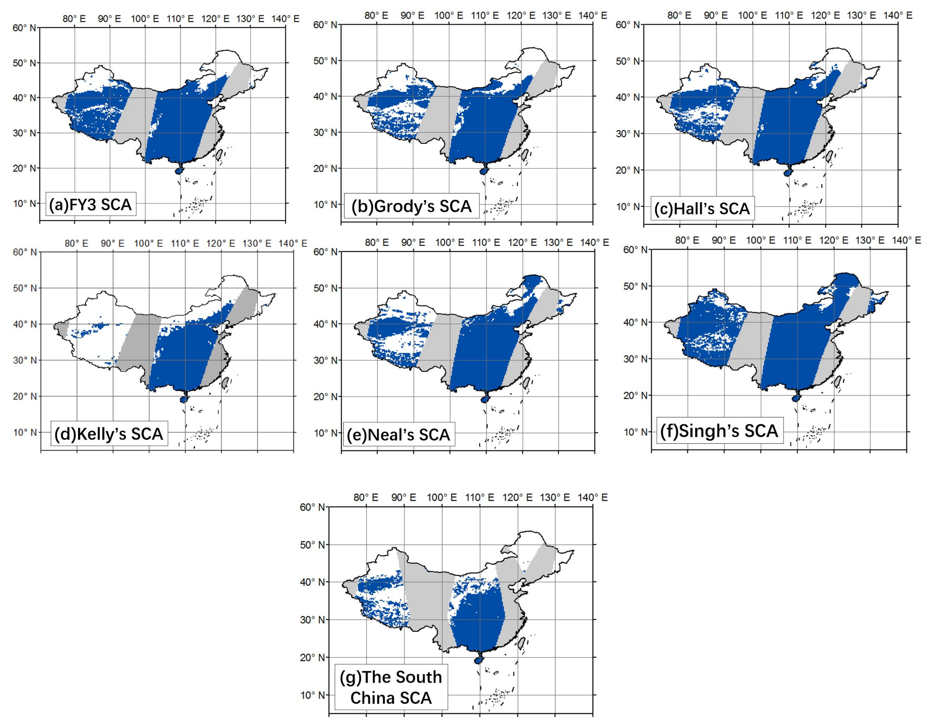
Tests were conducted for both ascending and descending data. The FY-3C/MWRI L1 swath data were resampled to a global equidistant cylindrical projection at 0.25° resolution for snow mapping. It should be noted that the South China algorithm identified snow using both ascending and descending data, resulting in a blended product for testing. The performances of the different PMW SCA maps for 7 January 2014 are shown in Figure 2. Snow extent determined using the seven methods clearly indicates the geographical distribution of snow over the three main seasonal snow-covered regions (Northwest, Northeast, and Tibetan Plateau). All methods achieved similar SCA estimations in the Northwest and the Northeast except for Singh’s algorithm, which missed significant snow. Over the Tibetan Plateau, the Kelly SCA algorithm tended to identify more snow. The FY3 algorithm and Singh algorithm, in contrast, estimated less snow.
For each algorithm, OA, PPV, OE and CE were calculated for the testing periods. Table 3 summarizes the evaluation results. For each algorithm, 276,946 station records were used for evaluating the ascending PMW SAC mapping results, and 275,774 station records were used for the descending data. Compared to in situ SD observations, all methods achieved a high OA ranging from 0.895 to 0.950. Grody’s algorithm, the South China algorithm and Kelly’s algorithm have higher PPV values (from 0.656 to 0.827) and lower OE values (from 0.173 to 0.344). Singh’s algorithm, Hall’s algorithm and Neal’s algorithm, with higher OE (from 0.492 to 0.860) and lower PPV (from 0.140 to 0.508) values, severely underestimated SCA during the testing periods. The descending orbit shows lower PPV and CE but higher OE than that of the ascending orbit. Because the local times on the ascending node and descending node are near 10:00 p.m. and 10:00 a.m., respectively, microwave brightness temperature at a high frequency may be more affected by atmospheric conditions during the descending orbits than during ascending orbits [33,36]. In addition, snow would melt during the day (descending orbit), and moist or wet snow is difficult to separate from land, which may lead to an increasing OE and decreasing PPV. Soil tends to be frozen during cold nights (ascending orbit), and it is difficult to separate frozen soil from dry snow, resulting in a higher CE. Evaluation results using IMS snow cover data as a reference are similar to the case using station observations. Whereas compared to evaluation results based on in situ observations, the results based on IMS snow cover product show higher classification error. The possible reasons for this difference include (i) the differences in the resolution of the evaluation datasets (i.e., point scale vs. image scale); (ii) the different snow types of the two datasets: only dry snow records of in situ observations were used for analysis, but IMS maps show both dry and wet snow; and (iii) errors in the IMS snow cover product. The performance of the IMS snow cover product deteriorates when identifying snow-free areas [37]. IMS is likely to overestimate snow cover in rugged terrain and tends to map more snow when the snow cover is patchy [31].
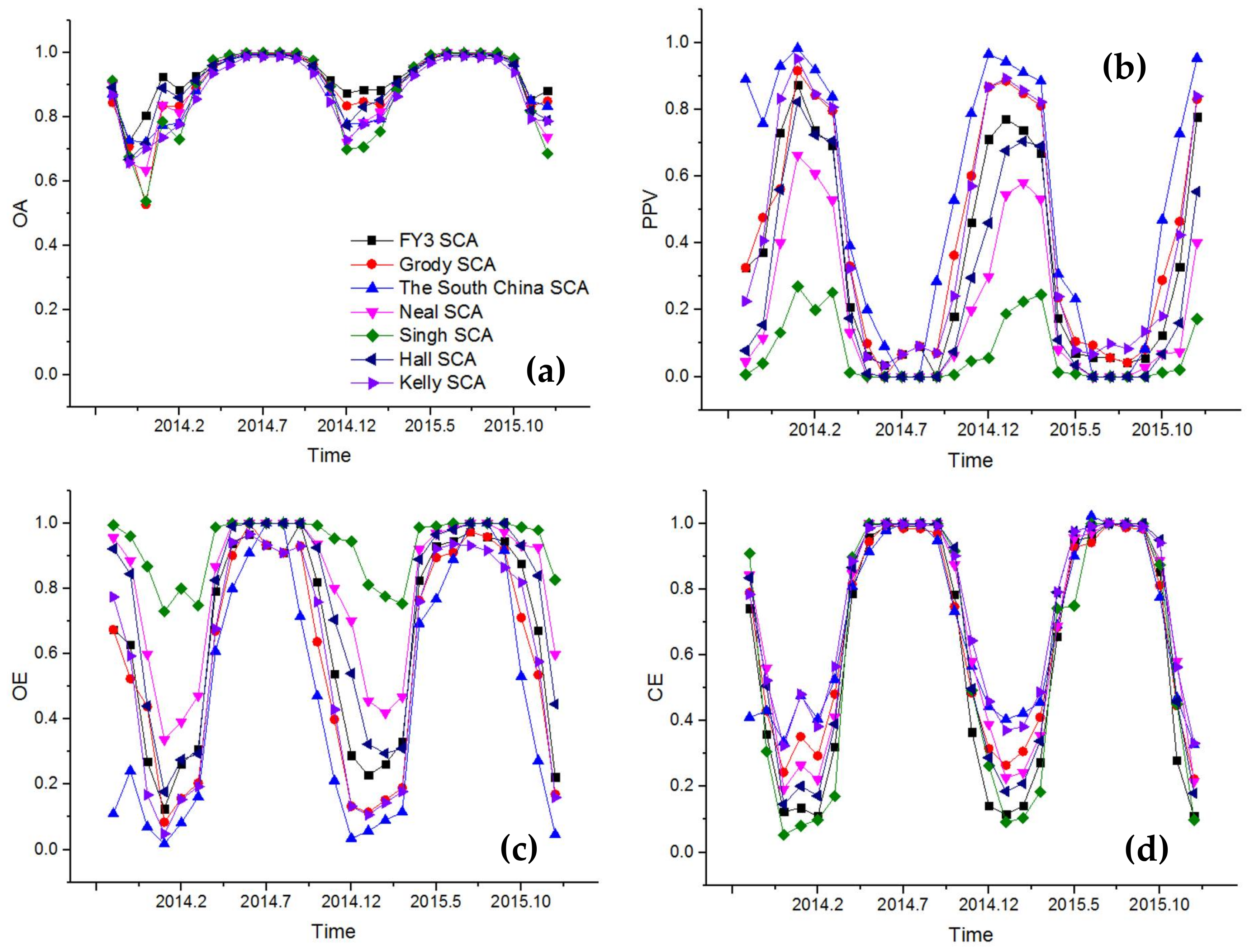
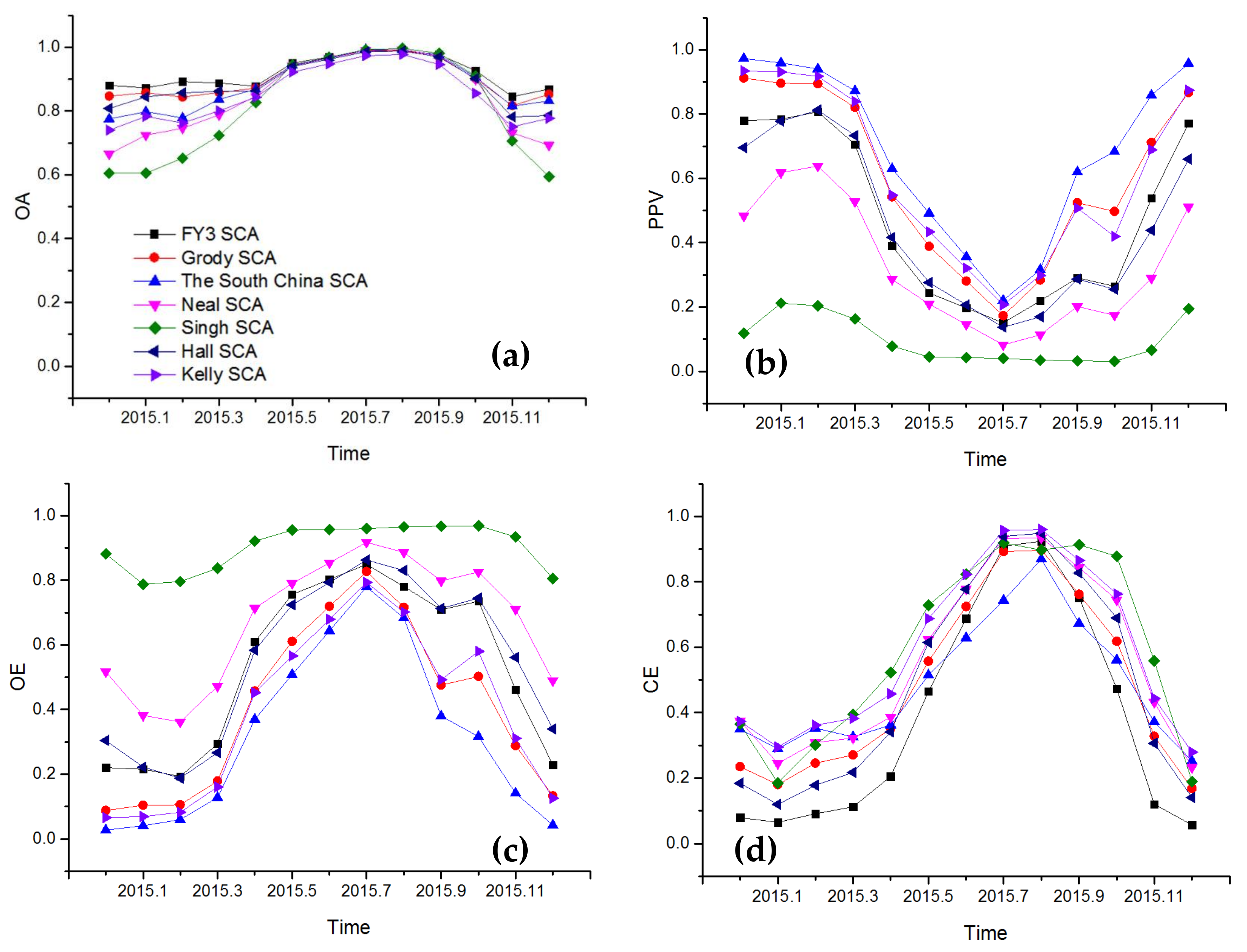
Monthly OA, OE, CE and PPV present a clear seasonal pattern as shown in Figure 3 and Figure 4. The OA of all algorithms is mostly high throughout the testing periods, and it improves to nearly 1.0 during the summer months when most regions are snow-free. Snow cover is small and patchy during the shoulder seasons (i.e., autumn, spring, and summer) leading to deteriorating capability of all PMW SCA mapping algorithms to detect snow. The OE and CE for all methods increase during the shoulder seasons when snow is accumulating or melting. During winter, the OE and CE of the seven algorithms mostly decrease to less than 0.5, and the PPV exceeds 0.5. Overall, the performance of the seven algorithms is comparable except for that of Singh’s algorithm, which exhibits larger errors than the others.
3.1. Effect of Land-Cover Types on Snow Cover Mapping Accuracy
The seven SCA identification algorithms presented in this study are all based on the decision tree approach with fixed threshold filters. The thresholds remain constant within different land-cover types. Because microwave radiation characteristics are related to land-cover types [13], the constant thresholds may introduce errors into classification. Therefore, it is necessary to identify the effects of land cover on PMW SCA mapping accuracy. Cropland, forest, grassland, and barren are the main land-cover types of seasonal-snow-dominated regions in China [38]. Their influences on snow mapping accuracy were analyzed using the land-cover map and in situ observational data.
The land-cover map (Figure 5) used in this study is a resampled product from the Globeland30 land-cover map. The Globeland30 land-cover map was projected and resampled to the same projection as that of the PMW SCA maps using the majority method. The majority algorithm assigns the most popular values within the filter window as the label of a pixel. This provides a more interpretable sense of the majority of land-cover types within each filter window. Pixels with a major land-cover fraction less than 70% have been removed from analysis because they are dominated by more than one land-cover type.
Figure 6 shows the OA, CE, PPV and OE of seven PMW SCA maps against station observations over barren, grassland, cropland and forests. As seen in Figure 6, the OA of all algorithms is not sensitive to land-cover type. Except for the South China algorithm, the CE of all algorithms over barren land and grasslands is higher than over the other land-cover types. The misclassification over barren land and grasslands may be a result of the difficulty in separating snow from frozen ground. Snow and frozen ground are scattering materials and have similar microwave radiation characteristics, making them difficult to distinguish. For the South China algorithm, severe omission error occurred over barren land versus other types of land cover. The OE in the FY algorithm and Grody’s algorithm is not sensitive to land-cover type. For Hall’s algorithm, Neal’s algorithm, Singh’s algorithm and Kelly’s algorithm, the OE is slightly higher over forested areas than over other land-cover types.
3.2. Effect of SCF on Snow-Cover Mapping Accuracy
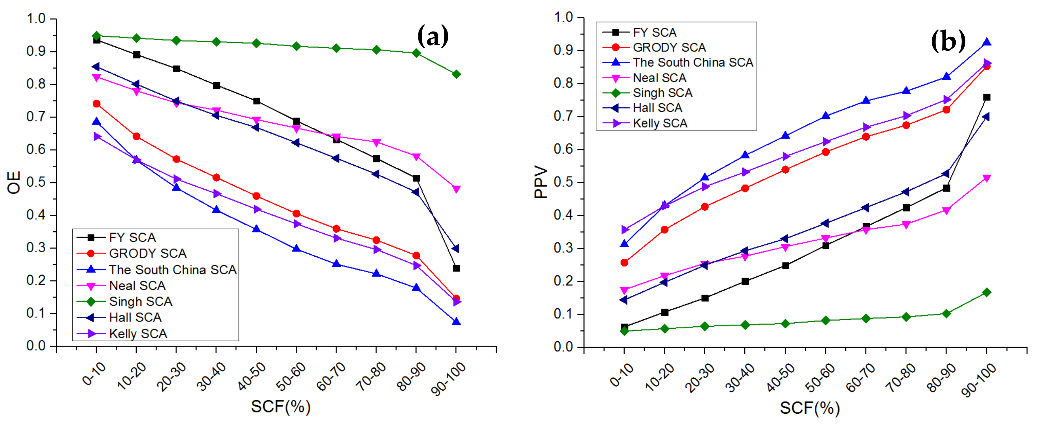
PMW SCA detection methods provide a binary snow classification that is sensitive to SCF [7,32]. Pixels with low SCF would be hard to detect using binary methods as the lack of snow signals can be captured by satellite sensors. The SCF values at 0.25° resolution were calculated using the one-kilometer IMS snow-cover product. Because only the snow-covered pixels (SCF > 0) were part of the analysis, the indexes OE and PPV were used for assessment. Figure 7 shows the statistics of OE and PPV associated with SCF. An increase in SCF from 0 to 100% results in a linear decline in underestimation of snow cover. In contrast to OE, values of PPV increase with increased SCF. Generally, the binary SCA product derived from optical remote sensing intends to indicate snow when the pixel’s snow cover exceeds 50% [7,32]. The PMW binary SCA does have apparent omission errors of less than 50% snow cover as shown in Figure 7. Though the IMS product has the problem of overestimating snow cover [31], it is still reasonable to believe that PMW binary SCA algorithms are sensitive to SCF, and their capability to estimate snow cover improves with higher SCF.
3.3. Effect of SD on Snow Cover Mapping Accuracy
Previous studies have shown the relationship between SD and the accuracy of SCA products: the accuracy of SCA decreases with decreasing SD [39,40]. In this study, we found a similar relationship between SD and PMW SCA. In addition, we found different effects of SD on the seven PMW SCA mapping methods.
Figure 8 presents the PPV and OE of the snow-cover maps for different SD ranges. Observed SD data were divided into six categories: SD < 5 cm, SD = 5–15 cm, SD = 15–25 cm, SD = 25–35 cm, SD = 35–45 cm and SD > 45 cm. The omission errors of the seven PMW SC maps show similar responses to SD ranges. The OE for all algorithms was highest when SD is less than five centimeters and tended to decline as SD exceeded five centimeters. This can be explained by the positive relation between SD (or SWE) and snow-cover fractions [41,42]. When snow surrounding the station is shallow, snowfall events are more likely to occur within a small area of the sensor’s field of view. Under this situation, pixels tend to be classified as snow-free generating increased OE. In contrast, when SD observed by station is quite high, pixels tend to be entirely covered by snow resulting in a decreased possibility of underestimation. PPV for all algorithms was lowest when SD is less than five centimeters. PPV values were nearly greater than 0.7 for the FY3 algorithm, Grody’s algorithm, the South China algorithm and Kelly’s algorithm when SD is greater than five centimeters. Variations in PPV of Grody’s algorithm and Kelly’s algorithm were less affected by SD than that of the other algorithms. These results indicate that Grody’s algorithm and Kelly’s algorithm are less sensitive to SD than the other algorithms.
4. Discussion
In this study, the performances of seven PMW SCA mapping methods in China were evaluated using in situ snow depth measurements and the one-kilometer IMS snow-cover product. The purpose of the study was to evaluate the differences among the PMW SCA mapping algorithms and to identify the influencing factors on the algorithms. Previous studies have demonstrated several difficulties in evaluating satellite-derived snow cover [30,31,32,39]. The use of point data and high-resolution SCA products for evaluation are both problematic [43]. Which data source is better for validation needs further study. However, to date, they are still the most reliable and useful validation datasets for evaluating satellite-derived SCA products [8,11,29,32].
All tested methods are based on the decision tree approach. The different SCA estimations are attributed to various classification criteria. Criteria for identifying various types of snow may lead to different positive predictive values and commission errors. Criteria for non-snow type identification such as precipitation and cold desert may introduce omission errors into snow identification. To determine whether these criteria can separate snow from other features accurately, the performances of the criteria in each algorithm as listed in Table 1 were tested using in situ data as described in Section 4.1. In addition, a classification structure of a decision tree was made of various nodes [44]. For PMW SCA detection, the nodes of the decision tree were mostly constructed by a selected multi-band combination of Tb or single-band Tb (hereafter termed Tb index) and the given thresholds. Proper Tb indexes and thresholds would exactly and accurately separate snow cover from other features. The performances and effects of Tb indexes and thresholds used in the seven PMW SCA mapping algorithms were analyzed and are described in Section 4.2, Section 4.3 and Section 4.4.
It should be noted that this study tended to evaluate the capability of each tested algorithm on snow identification, rather than on other feature classification. Thus, we only tested and assessed the performance of each criterion on snow identification. The classification accuracy of non-snow features such as precipitation, frozen ground, etc. are not discussed in this paper.
4.1. Criteria of PMW SCA Algorithms
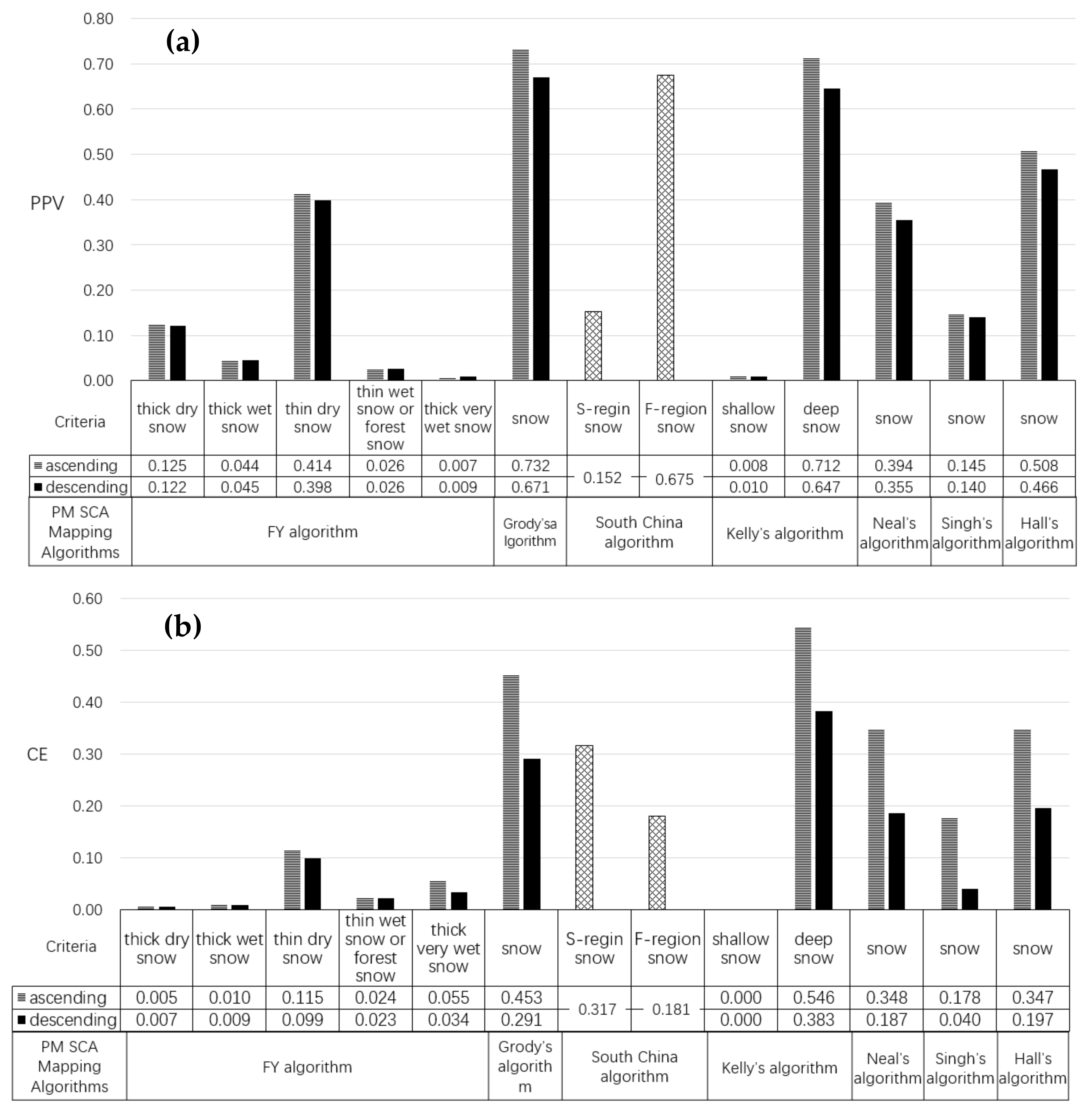
Criteria of the testing PMW SCA algorithms for assessment are listed in Table 1. Evaluation results are shown in Figure 9. For the FY3 algorithm, the criterion for thin dry snow had a much higher PPV and slightly higher CE than that of the other four criteria. Therefore, the thin dry snow criterion could be regarded as a more effective criterion than the other four criteria for snow identification in China. The criteria of Grody’s algorithm for snow identification and Kelly’s algorithm for deep snow identification had higher PPV values (>0.65) but introduced large commission errors. For Grody’s algorithm, the OE caused by the non-snow identification criteria was very small (<0.023) except for the precipitation filter, which is the major OE source. Both the PPV and CE of the shallow snow criterion of Kelly’s algorithm were near zero. These results indicated that the shallow snow criterion was essentially useless for snow detection in China. The South China algorithm designed two sets of criteria for identifying snow in forest- or dense-vegetation-covered regions (F-region) and sparse-vegetation regions (S-region), respectively. Testing results showed that the F-region snow criteria, with a higher PPV (>0.67) and lower CE (<0.18), performed much better than the S-region snow criteria. The commission errors of the South China algorithm were mainly attributed to the S-region snow criterion. The omission errors caused by each non-snow criterion were small (<0.14). The frozen ground filters were the major OE source of the South China algorithm, and this could be an important reason why severe omission errors occurred over barren rather than other types of land cover. Singh’s algorithm, Hall’s algorithm and Neal’s algorithm have shown apparent underestimation issues as shown in Figure 9, especially for Singh’s algorithm. The OE of Singh’s algorithm reached 0.86, the highest of the seven algorithms. Otherwise, the differences in error characteristics between ascending and descending data are identical to the conclusion described in Section 3.
4.2. Tb Indexes of PMW SCA Algorithms
The ideal Tb index should exactly separate snow cover from snow-free land. This means the Tb index values for snow and non-snow should be completely different. The decision tree would have better classification if its Tb indexes had significantly different values for snow and non-snow.
The Tb indexes used in the seven tested algorithms can be divided into five classes: single-band Tb, Tb gradient, polarization difference, polarization ratio and day–night Tb difference indexes. The five classes of Tb indexes and their values for snow and non-snow are shown in Figure 10. Snow, as a typical cold scattering material, has lower Tb values than the absorbing material (moist soil, vegetation, etc.). The Tb of snow decreases with increasing frequency. Thus, single-band Tb indexes and Tb gradient indexes are mainly used to identify snow from other absorbing or warm materials [16,35]. As expected, values of the single-band Tb indexes for snow and non-snow are largely different (Figure 10). These results demonstrate the availability of the single-band Tb indexes for snow discrimination. Most of the Tb gradient indexes have similar snow discrimination ability, except for (Tb23V − 0.49 × Tb89V). The index (Tb23V − 0.49 × Tb89V) has been used for filtering precipitation [16,17]. In this study, precipitation is considered non-snow. The range of (Tb23V − 0.49 × Tb89V) for snow entirely contains non-snow. This means snow would be barely separable from any other features (including precipitation) using this index. The failure of (Tb23V − 0.49 × Tb89V) in this study may have been caused by the insufficient training and analysis data for a global algorithm development [16,35]. Previous studies have proven that the polarization difference at 19 GHz for cold desert was greater than that of snow [16,18,35]. In this study, there is no observation station in desert. The index (Tb19V–Tb19H) presents little effect on snow discrimination. This is reasonable because the polarization difference for various absorbing materials and scattering materials could be the same, although their scattering characteristics are different [16,45]. The capability of the polarization difference index at 19 GHz should be investigated based on reliable data in further studies. The day–night Tb difference index, the polarization difference and the polarization ratio index at 37 GHz compromised with the Tb gradient indexes can be used to filter wet snow [17,18,45,46]. Only dry snow station records have been used in this study. Therefore, we just tested their effect on dry snow detection. As seen in Figure 10, the three types of indexes previously mentioned do not divide snow from non-snow effectively because the index values for snow and non-snow are very similar. Further research needs to be completed to understand their effects on wet snow detection.
4.3. Thresholds of PMW SCA Algorithms
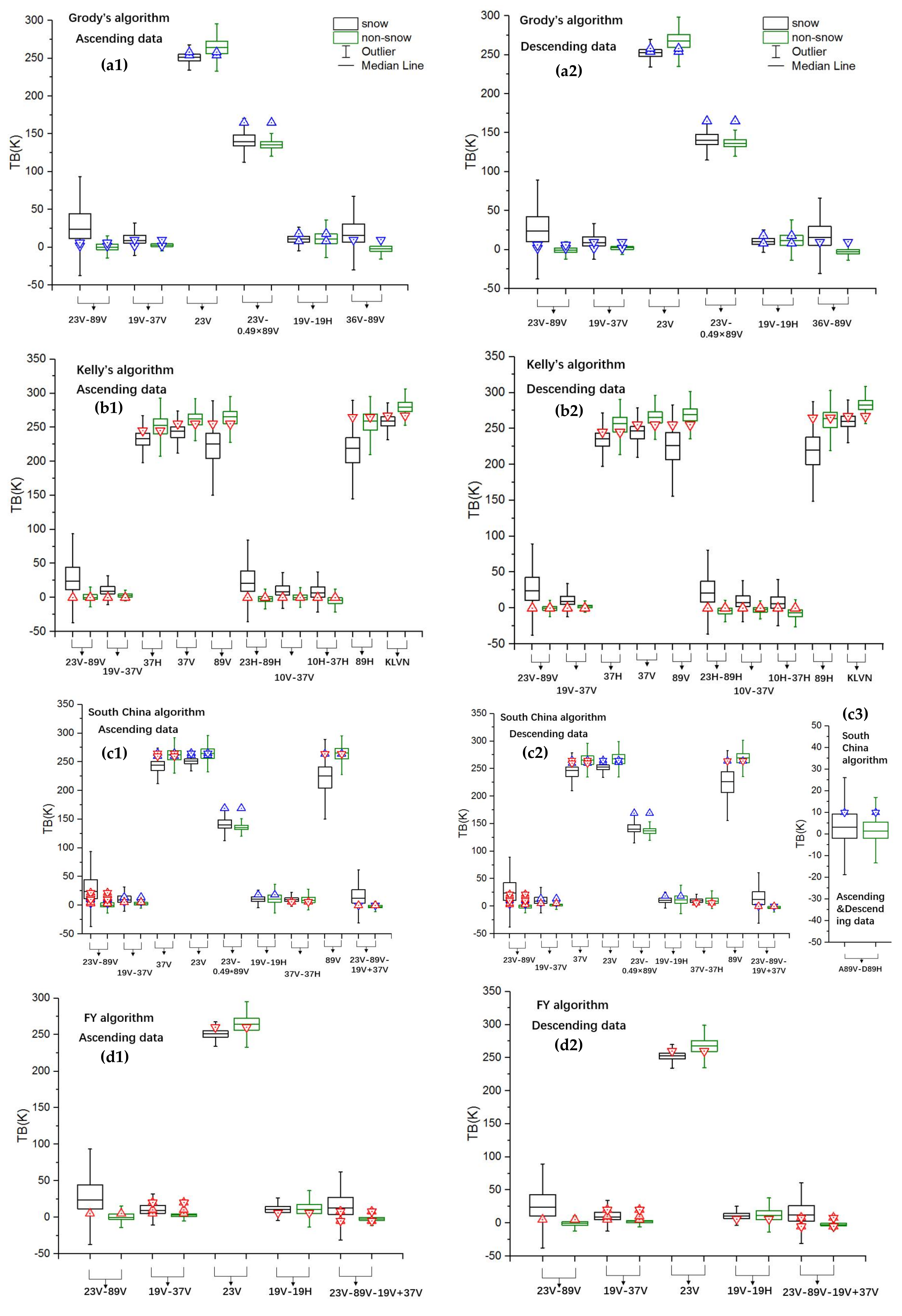
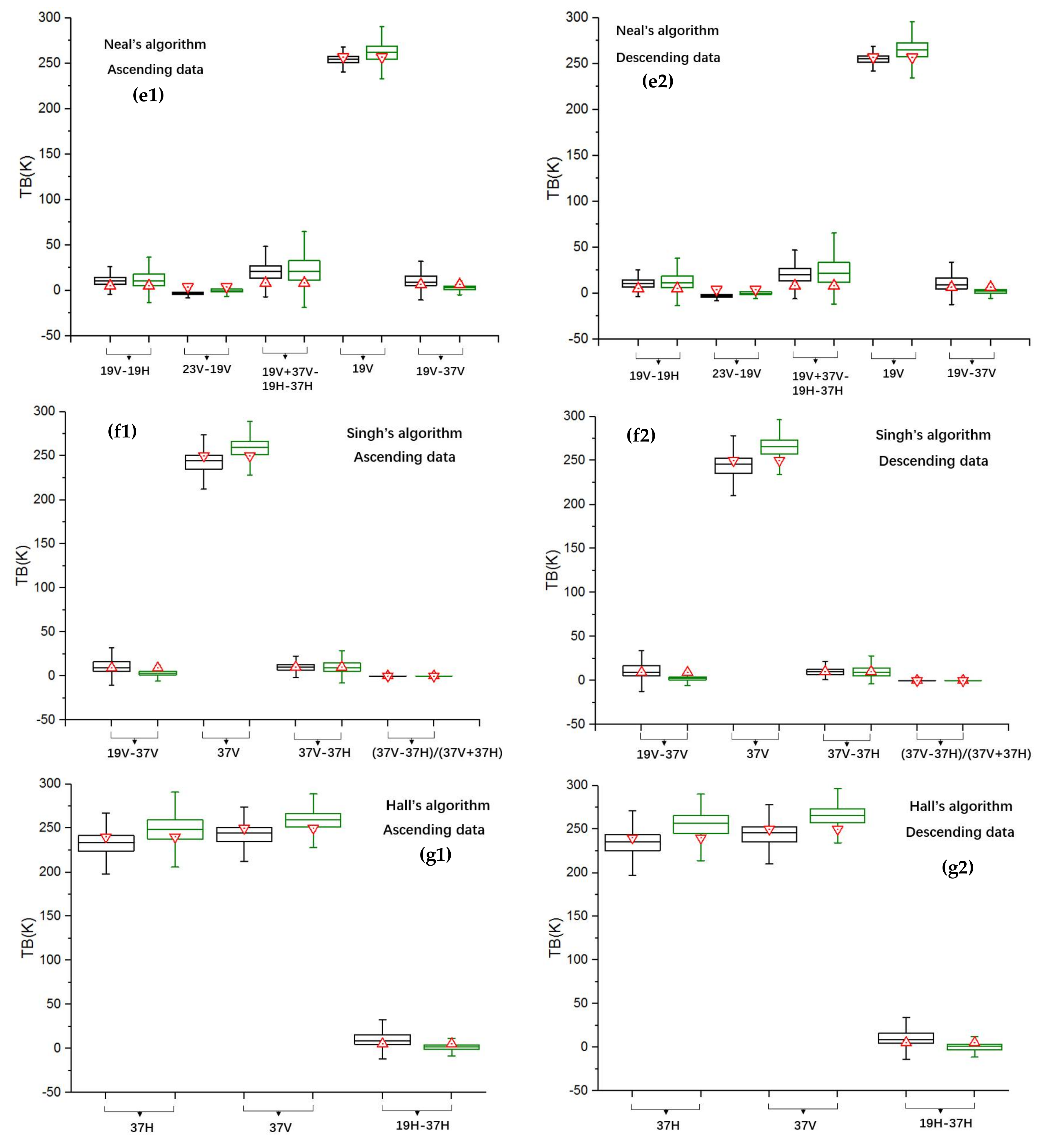
Thresholds are the other important factor in decision trees. Figure 11 summarizes the Tb indexes and thresholds used in the seven PMW SCA algorithms. Thresholds defined the upper bounds and lower bounds of the Tb index values for classification. The upper bounds for snow identification were mostly near the upper quartile of the snow box plots and lower quartile of the non-snow box plots. In contrast, the lower bounds for snow identification were mostly near the lower quartile of the snow box plots and the upper quartile of the non-snow box plots. These results mean nearly 75% of the snow could be detected and nearly 25% of the non-snow would be misclassified as snow. Similarly, the upper (lower) bounds for non-snow identification were mostly near the upper (lower) quartile of the non-snow box plots and the lower (upper) quartile of the snow box plots. These results mean nearly 75% of the non-snow could be successfully filtered and nearly 25% of the snow would be misclassified as non-snow.
4.4. Effects of Tb Indexes and Thresholds on PMW SCA Algorithms
The criteria for snow identification are essentially a compromising set of various filtering conditions [16]. The classification results are the compromising product of multiple conditions. The SCA mapping accuracy is attributed to all of the Tb indexes and thresholds used in the algorithm. The assessment results are described in Section 3 and can be explained based on the analysis of Tb indexes and thresholds.
Grody’s algorithm, the South China algorithm and Kelly’s algorithm have a higher PPV and a lower OE than the other algorithms. As seen in Figure 10 and Figure 11, it was found that most of the Tb indexes used in the Grody’s algorithm, the South China algorithm and Kelly’s algorithm have significantly different values for snow and non-snow. The proper Tb indexes provide a higher possibility for snow discrimination. In contrast, the relatively poorer discrimination ability of the Tb indexes for snow discrimination lead to misclassification, such as index (Tb23V − 0.49 × Tb89V). The performances of (Tb23V − 0.49 × Tb89V) used in Grody’s algorithm and the South China algorithm are unsatisfactory in this study. The index (Tb23V − 0.49 × Tb89V) should be an error source for the two algorithms. The thresholds are the other important error source of the algorithms. For example, most of the thresholds used in Kelly’s algorithm tended to identify more snow, resulting in higher PPV and CE. Similarly, the thresholds of Tb89V and (Tb23V − Tb89V − Tb19V + Tb37V) used in the South China algorithm were likely to overestimate SCA, leading to a higher PPV and CE. Compared to Grody’s algorithm, the South China algorithm and Kelly’s algorithm, the compromising set of criteria used in the FY3 algorithm is conservative for snow discrimination. It balances the problem between snow identification and overestimation. Though the conservative criteria for snow identification increases the OE, the FY3 algorithm still balances misclassification errors and snow identification well. As a result, the overall accuracy of the FY3 algorithm was the highest of all the tested algorithms.
The misclassification problem is severe for Neal’s algorithm, Singh’s algorithm and Hall’s algorithm. The three algorithms do not have typical criteria for identifying snow from other scattering materials, and they build conservative condition criteria for snow detection. The lack of filters and the strict criteria for snow are important error sources. In addition, there are some other triggers for misclassification. For Neal’s algorithm, its Tb indexes have a poor ability for snow discrimination (as seen in Figure 11). The threshold for the polarization ratio index (Tb37V − Tb37H)/(Tb37V + Tb37H) used in Singh’s algorithm seems too high and tends to misclassify snow as non-snow, leading to a high OE.
It was found that the thresholds and Tb indexes were identical for both ascending data and descending data as shown in Figure 10 and Figure 11. Though the difference between ascending data and descending data for most Tb indexes was small, the identical thresholds used in the algorithms still possibly generate false classification. Thus, the identical thresholds for ascending data and descending data may be a reason why ascending data and descending data resulted in a different performance.
As shown in Table 4, data for algorithm training and for the presented assessment work are from various satellite datasets, ground observation datasets and auxiliary datasets spanning different regions and years. A rich data source for algorithm development as for Grody’s algorithm can improve the stability of the algorithm. The South China algorithm and the FY3 algorithm were trained using Chinese local ground data. As a result, they were more likely to identify the land surface characteristics as compared to the remaining algorithms over China. This should be a reason for their good performance in the assessment.
The satellite data for developing the seven tested algorithms include AMSR-E data and SSM/I data. The Tb data used for evaluating the algorithms are from FY-3C/MWRI. The frequencies for MWRI are in accord with AMSR-E, and similar to SSM/I. MWRI, SSMI and AMSR-E have similar configurations. The difference between MWRI, SSMI and AMSR-E observations approximates to 0–2 K [47,48]. The impact of inter-sensor calibration issue is around −0.064–0.056 for OE and CE calculation, which has rarely affected the assessment results and conclusions shown in this paper. If the difference between various satellite measurements is obvious, an assessment of the impact of inter-sensor calibration issues should be carefully considered.
5. Conclusions
PMW SCA products are an important data source for snow cover monitoring. However, to date, uncertainty analysis for current PMW SCA mapping methods is rarely reported, especially in China. To investigate the performances of existing PMW SCA mapping algorithms in China, a thorough quantitative assessment of seven PMW SCA mapping algorithms in China was conducted in this study. Taking in situ SD observations and IMS snow cover as “ground truth” references, we compared the results of the PMW SCA maps derived from the seven algorithms.
Evaluation results for the PMW SCA maps showed the OA to be generally greater than 0.713 and 0.895 with respect to IMS and in situ observations, respectively. Grody’s algorithm, the South China algorithm and Kelly’s algorithm had higher positive predictive values and lower omission errors than the remaining studied algorithms. Their major error sources were the commission errors, which means they tended to estimate more snow. The FY3 algorithm estimated snow conservatively to reduce these commission issues. The overall accuracy of the FY3 algorithm was the highest of all the tested algorithms. Because of their conservative criteria for snow detection and the lack of filters for eliminating non-snow scattering materials, Singh’s algorithm, Hall’s algorithm and Neal’s algorithm had greater misclassification errors. The descending orbit exhibited a larger PPV, OA, and CE but a smaller OE for all of the algorithms. The difference in SCA accuracy between the descending and ascending orbits may be driven by the different atmospheric conditions and daily freeze/thaw cycles. The OA, OE and CE of each algorithm showed a clear seasonal pattern, decreasing at the onset of winter and increasing as the shoulder seasons progressed, while the PPV had the opposite seasonal trend.
The effects of land-cover type, SCF and SD were also analyzed in this study. The results indicated that serious underestimation of snow occurred over barren land and grasslands using the tested algorithms. All algorithms are sensitive to SCF and SD. However, Grody’s algorithm and Kelly’s algorithm are less sensitive to SD than the other algorithms. The capability of the PMW SCA mapping methods improved as SCF increased as well as when the SD exceeded five centimeters.
In addition, we analyzed each criterion used in the seven PMW SCA mapping algorithms. The characteristics of the Tb indexes and thresholds used in the tested PMW SCA algorithms were dissected. We found that some criteria used in the algorithms did not work effectively as designed. The failure criteria had a slight contribution to snow identification or introduced large classification errors. Revising the failure Tb indexes and thresholds would be a means to improve the algorithms. For example, the omission error is the main error course of FY algorithm. Extending the snow criteria of FY algorithm is the proposed method to reduce its omission error. For Kelly’s algorithm, Grody’s algorithm and the South China algorithm, their main error source is the commission error. It means these three algorithms tend to overestimate snow. Tightening their criteria for snow may reduce their omission error and improve their accuracy. Our analysis can be useful in understanding the uncertainties and the weaknesses of different PMW SCA mapping algorithms. The results shown in this study can be useful in developing new methods and can be taken as a reference when using PMW SCA products in different applications.
Acknowledgments
This study was supported by the National Natural Science Foundation of China (41671334), the Science & Technology Basic Resources Investigation Program of China (2017FY10052), the National Basic Research Program of China (2015CB953701) and the Strategic Pionner Program on Space Science, Chinese Academy of Sciences (XDA15052300). The authors would like to thank the China Meteorological Administration, National Geomatics Center of China, National Snow and Ice Data Center and US Geological Survey for providing meteorological station data, land-cover products and satellite data.
Author Contributions
Lingmei Jiang conceived and designed the study; Shengli Wu provided the FY-3C/MWRI data; Xiaojing Liu analyzed the data and wrote the results; Shirui Hao, Gongxue Wang and Jianwei Yang contributed analysis tools and methods.
Conflicts of Interest
The authors declare no conflict of interest.
Abbreviations
| PMW | Passive microwave |
| SCA | Snow cover area |
| SCF | Snow cover fraction |
| SD | Snow depth |
| SWE | Snow water equivalent |
| Tb | Brightness temperature |
| DTb | Brightness temperature of descending orbit |
| ATb | Brightness temperature of ascending orbit |
| 10 H, 18 H, 23 H, 37 H, 89 H | Brightness temperatures at the frequencies of 10.65 GHz, 18.7 GHz, 23.8 GHz, 36.5 GHz and 89.0 GHz for horizontal polarization |
| 10 V, 18 V, 23 V, 37 V, 89 V | Brightness temperatures at the frequencies of 10.65 GHz, 18.7 GHz, 23.8 GHz, 36.5 GHz and 89.0 GHz for vertical polarization |
| ASCT = ATb23.8V − ATb89V − (ATb18.7V − ATb37.5V) | |
| KLVN = 58.08 − 0.39 × Tb19V + 1.21 × Tb23V − 0.37 × Tb37H + 0.36 × Tb89V | |
| F-region | Forest-covered region or dense-vegetation-covered region |
| S-region | Sparse-vegetation-covered region |
| OA | Overall accuracy |
| OE | Omission error |
| CE | Commission error |
| PPV | Positive predictive value |
References
- Liang, S. Advances in Land Remote Sensing: System, Modeling, Inversion and Application; Springer Science & Business Media: Houten, The Netherlands, 2008. [Google Scholar]
- AghaKouchak, A.; Farahmand, A.; Melton, F.S.; Teixeira, J.; Anderson, M.C.; Wardlow, B.D.; Hain, C.R. Remote sensing of drought: Progress, challenges and opportunities. Geophys. Res. 2015, 53, 452–480. [Google Scholar] [CrossRef]
- Frei, A.; Tedesco, M.; Lee, S.; Foster, J.; Hall, D.K.; Kelly, R.; Robinson, D.A. A review of global satellite-derived snow products. Adv. Space Res. 2012, 50, 1007–1029. [Google Scholar] [CrossRef]
- Dietz, A.J.; Kuenzer, C.; Gessner, U.; Dech, S. Remote sensing of snow—A review of available methods. Int. J. Remote Sens. 2012, 33, 4094–4134. [Google Scholar] [CrossRef]
- Frei, A.; Robinson, D.A. Northern hemisphere snow extent: Regional variability 1972–1994. J. Clim. 1999, 19, 1535–1560. [Google Scholar] [CrossRef]
- Dozier, J. Spectral signature of alpine snow cover from the landsat thematic mapper. Remote Sens. Environ. 1989, 28, 9–22. [Google Scholar] [CrossRef]
- Hall, D.K.; Riggs, G.A.; Salomonson, V.V.; DiGirolamo, N.E.; Bayr, K.J. MODIS snow-cover products. Remote Sens. Environ. 2002, 83, 181–194. [Google Scholar] [CrossRef]
- Painter, T.H.; Rittger, K.; McKenzie, C.; Slaughter, P.; Davis, R.E.; Dozier, J. Retrieval of subpixel snow covered area, grain size, and albedo from MODIS. Remote Sens. Environ. 2009, 113, 868–879. [Google Scholar] [CrossRef]
- Shi, J. An automatic algorithm on estimating sub-pixel snow cover from MODIS. Quat. Sci. 2012, 32, 6–15. [Google Scholar]
- Grody, N.C. Surface identification using satellite microwave radiometers. IEEE Trans. Geosci. Remote Sens. 1988, 26, 850–859. [Google Scholar] [CrossRef]
- Xu, X.; Liu, X.; Li, X.; Xin, Q.; Chen, Y.; Shi, Q.; Ai, B. Global snow cover estimation with microwave brightness temperature measurements and one-class in situ observations. Remote Sens. Environ. 2016, 182, 227–251. [Google Scholar] [CrossRef]
- Kongoli, C.; Romanov, P.; Ferraro, R. Snow cover monitoring from remote sensing satellites: Possibilities for drought assessment. In Remote Sensing of Drought: Innovative Monitoring Approaches; CRC Press: Boca Raton, FL, USA, 2012; pp. 359–386. [Google Scholar]
- Shi, J.C.; Xiong, C.; Jiang, L.M. Review of snow water equivalent microwave remote sensing. Sci. China Earth Sci. 2016, 59, 731–745. [Google Scholar] [CrossRef]
- Kelly, R. The AMSR-E snow depth algorithm: Description and initial results. J. Remote Sens. 2009, 29, 307–317. [Google Scholar]
- Li, X.; Liu, Y.; Zhu, X.; Zheng, Z.; Chen, A. Snow cover identification with SSM/I data in china. J. Appl. Meteorol. Sci. 2007, 18, 12–20. [Google Scholar]
- Grody, N.C.; Basist, A.N. Global identification of snowcover using SSM/I measurements. IEEE Trans. Geosci. Remote Sens. 1996, 34, 237–249. [Google Scholar] [CrossRef]
- Pan, J.; Jiang, L.; Zhang, L. In Wet snow detection in the south of china by passive microwave remote sensing. In Proceedings of the 2012 32nd IEEE International Geoscience and Remote Sensing Symposium, Munich, Germany, 22–27 July 2012; Institute of Electrical and Electronics Engineers Inc.: Munich, Germany, 2012; pp. 4863–4866. [Google Scholar]
- Singh, P.R.; Gan, T.Y. Retrieval of snow water equivalent using passive microwave brightness temperature data. Remote Sens. Environ. 2000, 74, 275–286. [Google Scholar] [CrossRef]
- Hall, D.K.; Kelly, R.E.; Riggs, G.A.; Chang, A.T.; Foster, J.L. Assessment of the relative accuracy of hemispheric-scale snow-cover maps. Ann. Glaciol. 2002, 34, 24–30. [Google Scholar] [CrossRef]
- Neale, C.M.U.; Mcfarland, M.J.; Chang, K. Land-surface-type classification using microwave brightness temperatures from the special sensor microwave/imager. IEEE Trans. Geosci. Remote Sens. 1990, 28, 829–838. [Google Scholar] [CrossRef]
- Liang, T.; Zhang, X.; Xie, H.; Wu, C.; Feng, Q.; Huang, X.; Chen, Q. Toward improved daily snow cover mapping with advanced combination of MODIS and AMSR-E measurements. Remote Sens. Environ. 2008, 112, 3750–3761. [Google Scholar] [CrossRef]
- Ramsay, B.H. The interactive multisensor snow and ice mapping system. Hydrol. Process. 1998, 12, 1537–1546. [Google Scholar] [CrossRef]
- Helfrich, S.R.; McNamara, D.; Ramsay, B.H.; Baldwin, T.; Kasheta, T. Enhancements to, and Forthcoming Developments in the Interactive Multisensor Snow and Ice Mapping System (IMS). Hydrol. Process. 2007, 21, 1576–1586. [Google Scholar] [CrossRef]
- Romanov, P. Global multisensor automated satellite-based snow and ice mapping system (GMASI) for cryosphere monitoring. Remote Sens. Environ. 2017, 196, 42–55. [Google Scholar] [CrossRef]
- Luojus, K.; Pulliainen, J.; Takala, M.; Kangwa, M.; Smolander, T.; Wiesmann, A.; Derksen, C.; Metsamaki, S.; Salminen, M.; Solberg, R.; et al. Globsnow-2 Product User Guide Version 1.0; European Space Agency Study Contract Report, ESRIN Contract 21703/08/I-EC; ESA/ESRIN: Frascati, Italy, 2013. [Google Scholar]
- Jiang, L.; Wang, P.; Zhang, L.; Yang, H.; Yang, J. Improvement of snow depth retrieval for fy3b-mwri in china. Sci. China Earth Sci. 2014, 57, 1278–1292. [Google Scholar] [CrossRef]
- Maeda, T.; Taniguchi, Y. Descriptions of GCOM-W1 AMSR-2 Level 1R and Level 2 Algorithms; Japan Aerospace Exploration Agency Earth Observation Research Center: Ibaraki, Japan, 2013. [Google Scholar]
- Chang, A.T.; Rango, A. Algorithm Theoretical Basis Document (ATBD) for the AMSR-E Snow Water Equivalent Algorithm; NASA/GSFC: Greenbelt, MD, USA, 2000. [Google Scholar]
- Hori, M.; Sugiura, K.; Kobayashi, K.; Aoki, T.; Tanikawa, T.; Kuchiki, K.; Niwano, M.; Enomoto, H. A 38-year (1978–2015) northern hemisphere daily snow cover extent product derived using consistent objective criteria from satellite-borne optical sensors. Remote Sens. Environ. 2017, 191, 402–418. [Google Scholar] [CrossRef]
- Romanov, P.; Gutman, G.; Csiszar, I. Automated monitoring of snow cover over North America with multispectral satellite data. J. Appl. Meteorol. 2000, 39, 1866–1880. [Google Scholar] [CrossRef]
- Chen, X.; Jiang, L.; Yang, J.; Pan, J. Validation of ice mapping system snow cover over southern china based on landsat enhanced thematic mapper plus imagery. J. Appl. Remote Sens. 2014, 8. [Google Scholar] [CrossRef]
- Rittger, K.; Painter, T.H.; Dozier, J. Assessment of methods for mapping snow cover from MODIS. Adv. Water Resour. 2013, 51, 367–380. [Google Scholar] [CrossRef]
- Lee, Y.K.; Kongoli, C.; Key, J. An in-depth evaluation of heritage algorithms for snow cover and snow depth using AMSR-E and AMSR2 measurements. J. Atmos. Ocean. Technol. 2015, 32, 2319–2336. [Google Scholar] [CrossRef]
- Siljamo, N.; Hyvärinen, O. New geostationary satellite-based snow-cover algorithm. J. Appl. Meteorol. Clim. 2011, 50, 1275–1290. [Google Scholar] [CrossRef]
- Grody, N.C. Classification of snow cover and precipitation using the special sensor microwave imager. J. Geophys. Res. Atmos. 1991, 96, 7423–7435. [Google Scholar] [CrossRef]
- Foster, J.L.; Hall, D.K.; Chang, A.T.C.; Rango, A. An overview of passive microwave snow research and results. Rev. Geophys. Space Phys. 1984, 22, 195–208. [Google Scholar] [CrossRef]
- Brubaker, K.L.; Pinker, R.T.; Deviatova, E. Evaluation and comparison of MODIS and IMS snow-cover estimates for the continental united states using station data. J. Hydrometeorol. 2005, 6, 1002–1017. [Google Scholar] [CrossRef]
- Wang, J.; Li, H.; Hao, X.; Huang, X.; Hou, J.; Che, T.; Dai, L.; Liang, T.; Huang, C.; Li, H.; et al. Remote sensing for snow hydrology in China: Challenges and perspectives. J. Appl. Remote Sens. 2014, 8. [Google Scholar] [CrossRef]
- Yang, J.; Jiang, L.; Menard, C.B.; Luojus, K.; Lemmetyinen, J.; Pulliainen, J. Evaluation of Snow Products over the Tibetan Plateau. Hydrol. Process. 2015, 29, 3247–3260. [Google Scholar] [CrossRef]
- Klein, A.G.; Barnett, A.C. Validation of daily MODIS snow cover maps of the Upper Rio Grande River Basin for the 2000–2001 snow year. Remote Sens. Environ. 2003, 86, 162–176. [Google Scholar] [CrossRef]
- Rittger, K.; Bair, E.H.; Kahl, A.; Dozier, J. Spatial estimates of snow water equivalent from reconstruction. Adv. Water Resour. 2016, 94, 345–363. [Google Scholar] [CrossRef]
- Romanov, P.; Dan, T.; Gutman, G.; Carroll, T. Mapping and monitoring of the snow cover fraction over North America. J. Geophys. Res. 2003, 108, 137–141. [Google Scholar] [CrossRef]
- Bitner, D.; Carroll, T.; Cline, D.; Romanov, P. An assessment of the differences between three satellite snow cover mapping techniques. Hydrol. Process. 2002, 16, 3723–3733. [Google Scholar] [CrossRef]
- Sharma, R.; Ghosh, A.; Joshi, P.K. Decision tree approach for classification of remotely sensed satellite data using open source support. J. Erath Syst. Sci. 2013, 122, 1237–1247. [Google Scholar] [CrossRef]
- Pan, J. Study of the Snow Detection Decision Tree Algorithm Using Passive Microwave Remote Sensing Technology in the South of China. Master’s Thesis, Beijing Normal University, Beijing, China, 2012. [Google Scholar]
- Walker, A.E.; Goodison, B.E. Discrimination of a wet snowcover using passive microwave satellite data. Ann. Glaclol. 1993, 17. [Google Scholar] [CrossRef]
- Wu, S.; Chen, J. Instrument performance and cross calibration of FY-3C MWRI. In Proceedings of the 36th IEEE International Geoscience and Remote Sensing Symposium, IGARSS 2016, Beijing, China, 10–15 July 2016; pp. 388–391. [Google Scholar]
- Yang, J.; Luojus, K.; Lemmetyinen, J.; Jiang, L.; Pulliainen, J. Comparison of SSMIS, AMSR-E and MWRI brightness temperature data. In Proceedings of the Joint 2014 IEEE International Geoscience and Remote Sensing Symposium, IGARSS 2014 and the 35th Canadian Symposium on Remote Sensing, CSRS 2014, Quebec City, QC, Canada, 13–18 July 2014; pp. 2574–2577. [Google Scholar]
Figure 1.
Chinese meteorological stations used in this work.
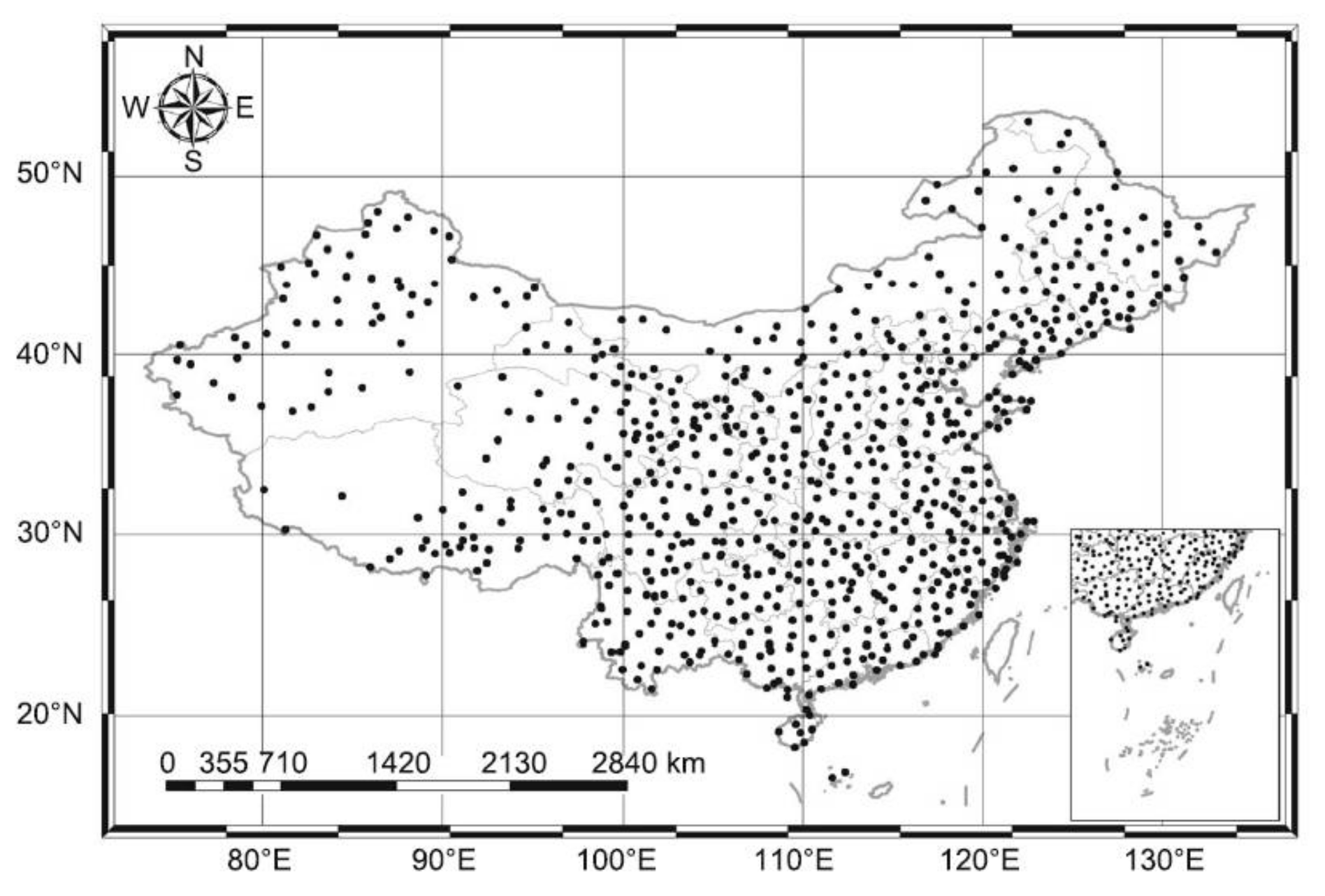
Figure 2.
Comparison of PMW SCA maps for 7 January 2014: (a) FY SCA map, (b) Grody’s SCA map, (c) Hall’s SCA map, (d) Kelly’s SCA map, (e) Neal’s SCA map, (f) Singh’s SCA map, (g) the South China SCA map. (blended SCA image (g) using both ascending and descending data for the South China algorithm and descending SCA images(a–f) for the remaining PMW SCA mapping algorithms).

Figure 3.
Monthly OA (a), PPV (b), OE (c) and CE (d) of the seven PMW SCA maps based on in situ SD observations.
Figure 3.
Monthly OA (a), PPV (b), OE (c) and CE (d) of the seven PMW SCA maps based on in situ SD observations.

Figure 4.
Monthly OA (a), PPV (b), OE (c) and CE (d) of the seven PMW SCA maps based on the IMS snow cover product.
Figure 4.
Monthly OA (a), PPV (b), OE (c) and CE (d) of the seven PMW SCA maps based on the IMS snow cover product.

Figure 5.
Globeland30 land-cover map.
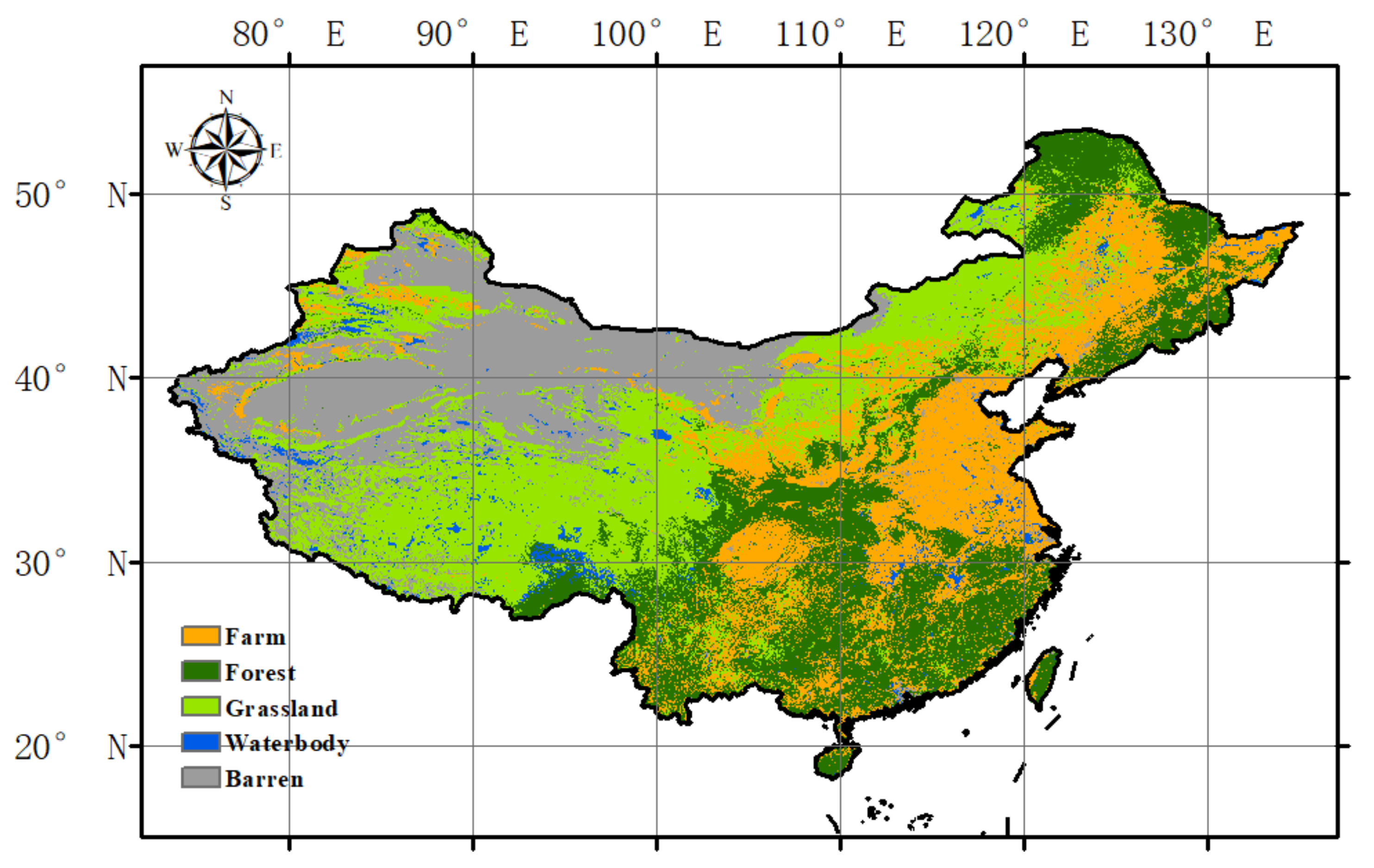
Figure 6.
OA (a), PPV (b), OE (c) and CE (d) of the seven PMW SCA maps compared to station observations in different land-cover types.
Figure 6.
OA (a), PPV (b), OE (c) and CE (d) of the seven PMW SCA maps compared to station observations in different land-cover types.
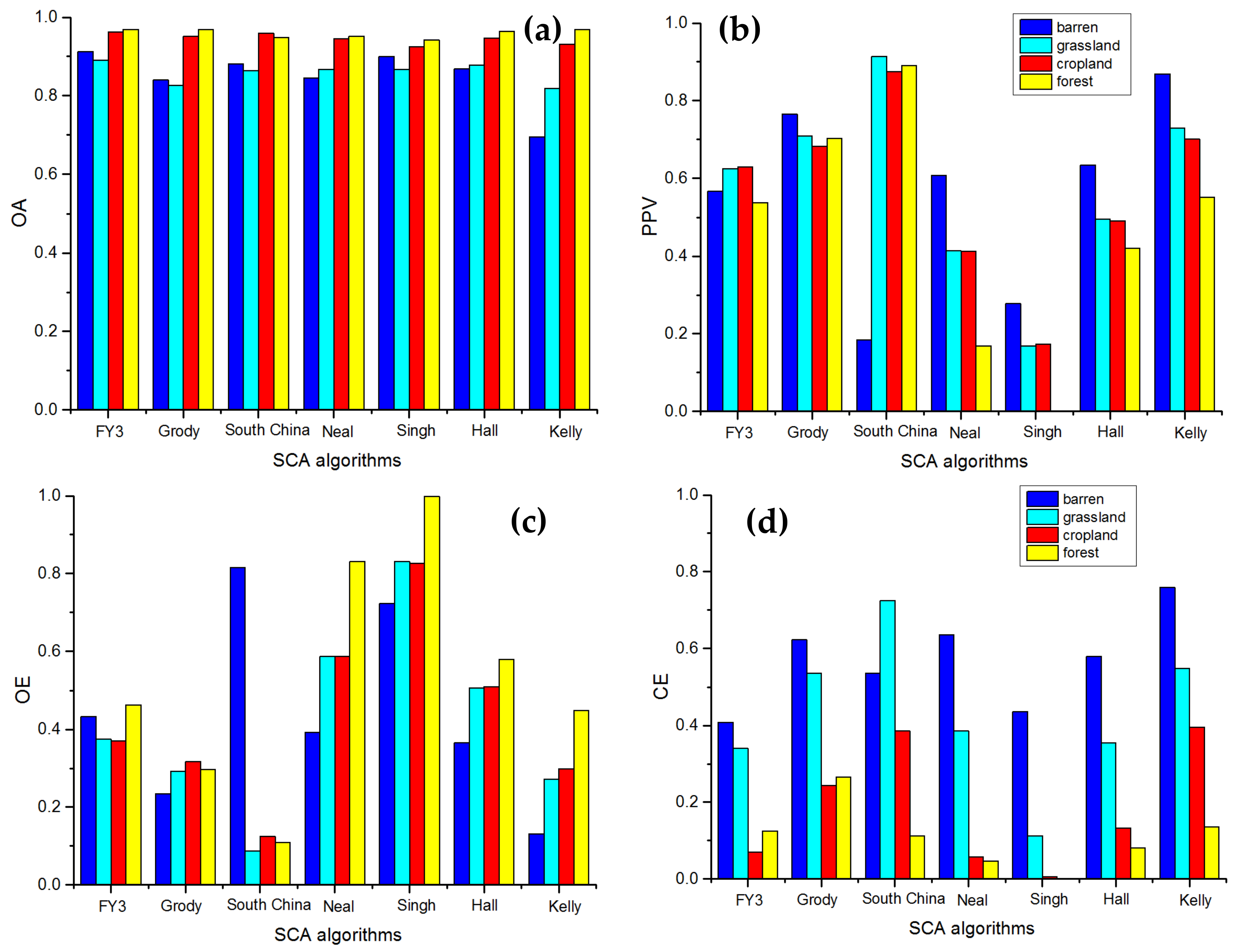
Figure 7.
OE (a) and PPV (b) of the PMW SCA mapping algorithms associated with different SCFs.

Figure 8.
OE (a) and PPV (b) of the seven PMW SCA maps compared to ground observations at different snow depths.
Figure 8.
OE (a) and PPV (b) of the seven PMW SCA maps compared to ground observations at different snow depths.
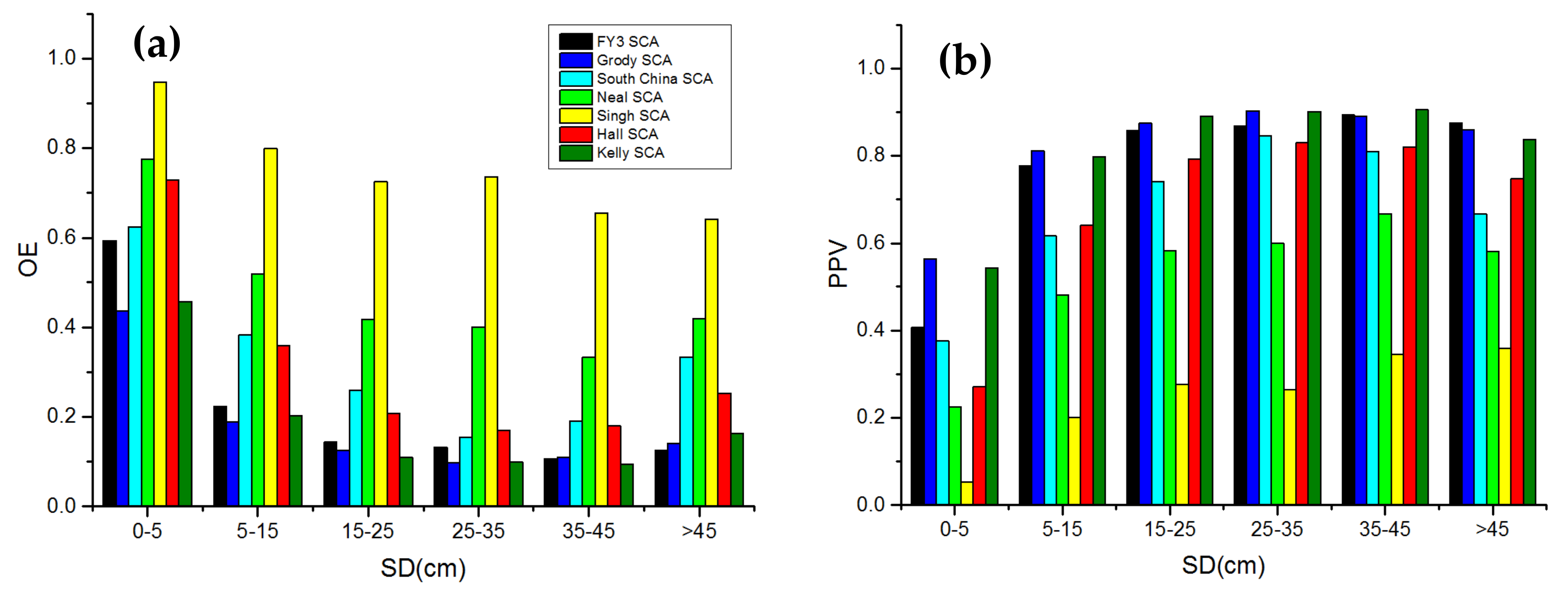
Figure 9.
The evaluation results of classification criteria for each algorithm: PPV (a), CE (b), OE (c).
Figure 9.
The evaluation results of classification criteria for each algorithm: PPV (a), CE (b), OE (c).

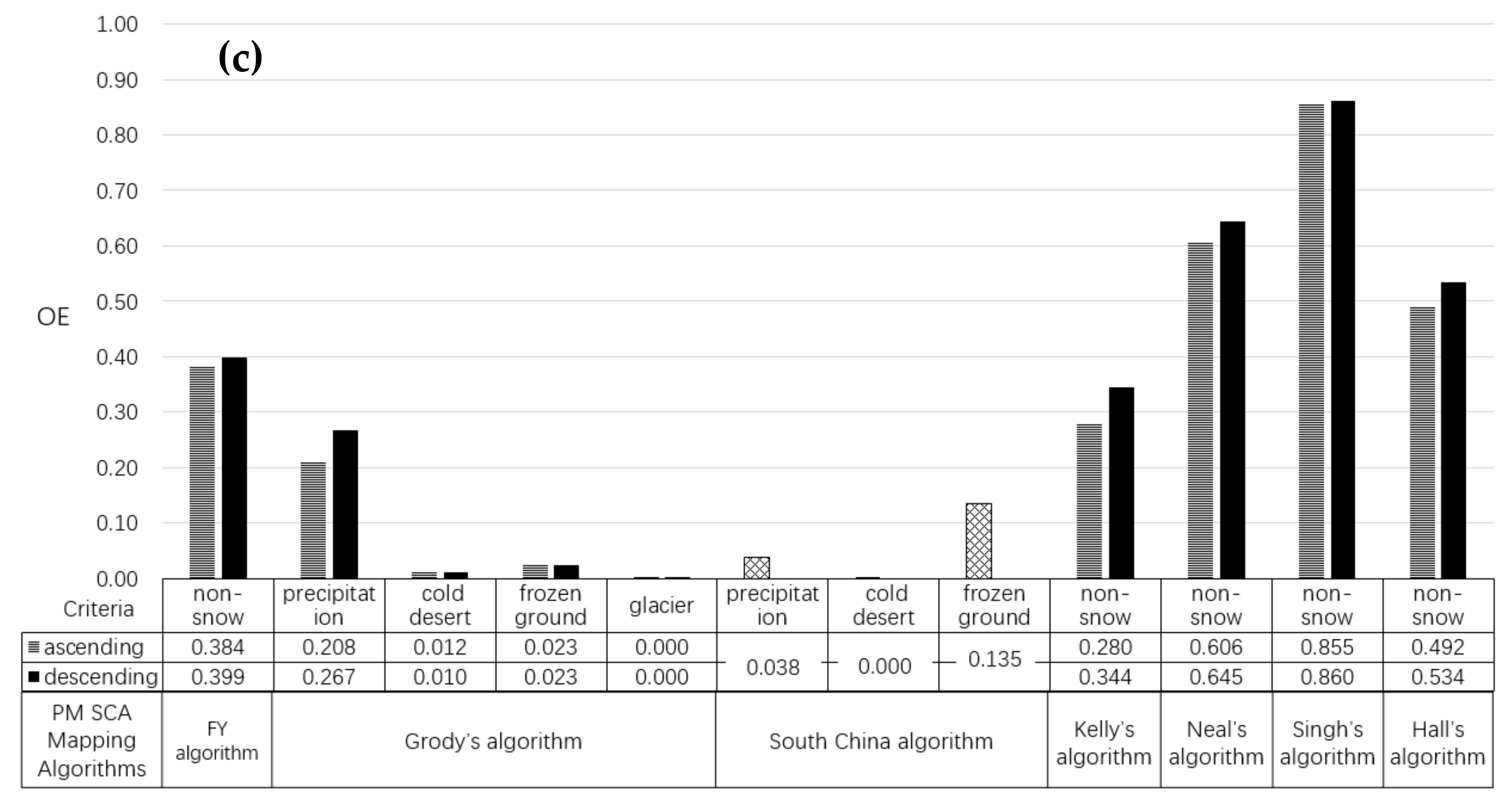
Figure 10.
Box plots of the single-band indexes (a1,a2), the Tb gradient indexes (b1,b2), the polarization difference indexes (c1,c2), the polarization ratio indexes(d1,d2) and the day–night Tb difference indexes (e).
Figure 10.
Box plots of the single-band indexes (a1,a2), the Tb gradient indexes (b1,b2), the polarization difference indexes (c1,c2), the polarization ratio indexes(d1,d2) and the day–night Tb difference indexes (e).
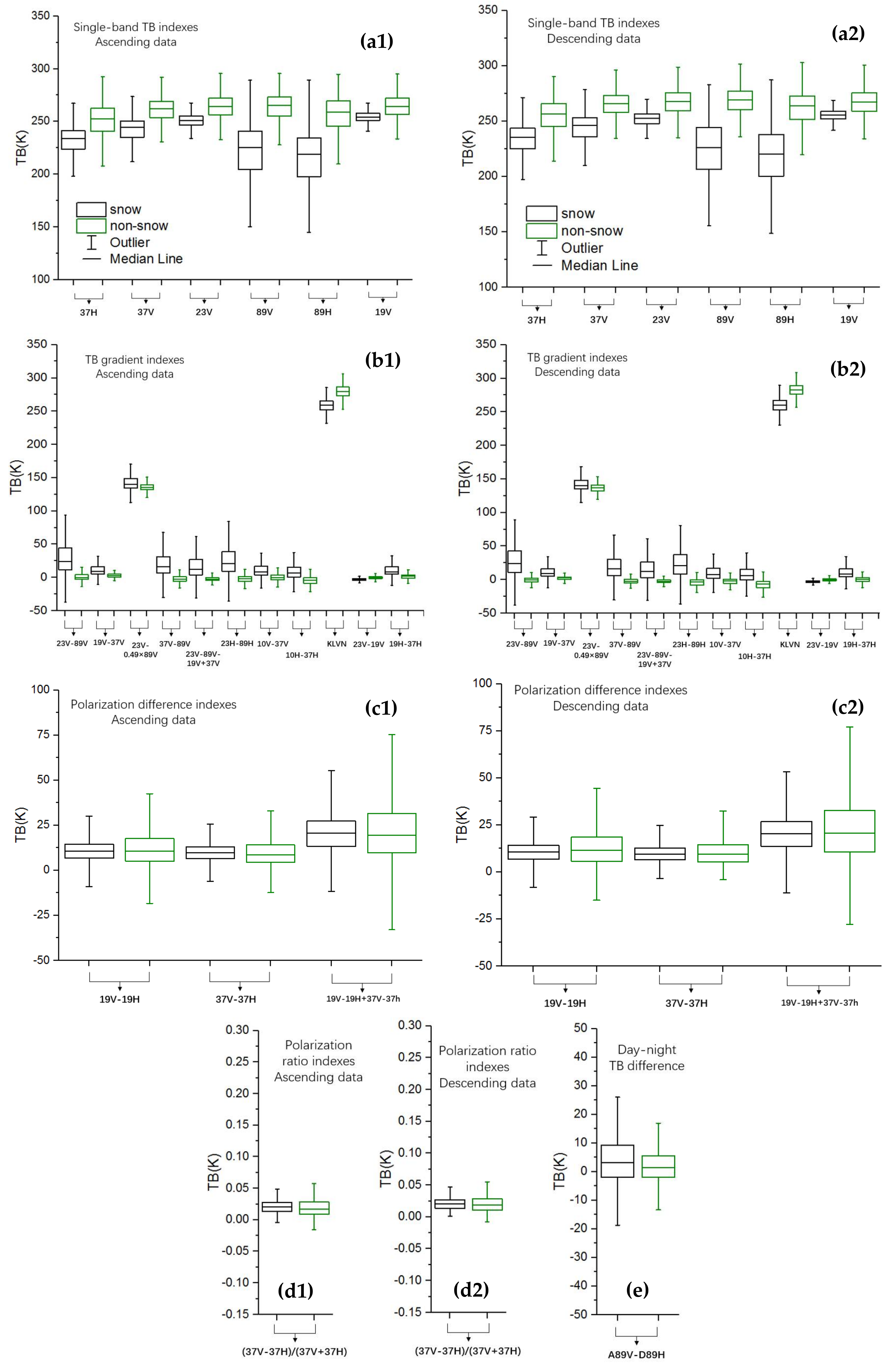
Figure 11.
Box plots of Tb index values and thresholds of the seven PMW SCA mapping algorithms: Grody’s algorithm (a1,a2), Kelly’s SCA algorithm (b1,b2), the South China algorithm (c1–c3), FY SCA algorithm (d1,d2), Neal’s algorithm (e1,e2), Singh’s algorithm (f1,f2), Hall’s algorithm (g1,g2). (The up and down arrows indicate the lower bounds and upper bounds of the thresholds, respectively. Arrows in red and in blue indicate thresholds for snow identification and non-snow identification, respectively.)


Table 1.
Classification criteria of passive microwave (PMW) snow cover area (SCA) mapping algorithms.
Table 1.
Classification criteria of passive microwave (PMW) snow cover area (SCA) mapping algorithms.
| Methods | Classification Criteria | Remark | ||||
|---|---|---|---|---|---|---|
| Grody‘s algorithm | Scattering materials: Tb23V − Tb89V > 0 or Tb19V − Tb37V > 0 | |||||
| Snow: | Non-snow | |||||
| Do not meet the criteria of non-snow | Precipitation | (Tb23V ≥ 258) or (Tb23V ≥ 165 + 0.49 * Tb89V) or (254 ≤ Tb23V ≤ 258.0 & (Tb23V − Tb89V ≤ 2 or Tb19V − Tb37V ≤ 2)) | ||||
| Cold Desert: | (Tb19V − Tb19H ≥ 18) & (Tb19V − Tb37V ≤ 10) & (Tb37V − Tb89V ≤ 10) | |||||
| Frozen ground | (Tb19V − Tb19H ≥ 8) & (Tb23V − Tb89V) ≤ 6 & (Tb19V − Tb37V) ≤ 2 | |||||
| Glacier | (Tb23V ≤ 229 & Tb19V − Tb19H ≥ 23) or (Tb23V < 210) | |||||
| South China algorithm | Scattering materials: DTb23V − DTb89V > 5 or DTb19V − DTb37V > 5 | DTb: descending orbit ATb: ascending orbit ASCT = ATb23.8V − ATb89V − (ATb18.7V − ATb37.5V) F-: Forest-covered region or dense vegetation coverd region S-: Sparse-vegetation region | ||||
| Snow | Non-snow | |||||
| S-region snow: | (DTb23V − DTb89V≥22) or (DTb23V − DTb89V < 22 & DTb37.5V < 260 & DTb37V − DTb37H ≥ 6) & (DTb23V − DTb89V ≥ 12 or (DTb23V − DTb89V < 12 & ATb37V < 265 & ASCT ≥ 0)) | Precipitation: | (DTb23V ≥ 265) or (DTb23V ≥ 169 + 0.5 * DTb89V) or ((DTb23V − DTb89V ≤ 6 or DTb18V − DTb37V ≤ 6) or (261 ≤ DTb23V ≤ 265)) | |||
| Cold Desert: | (DTb18V − DTb18H ≥ 18) & (DTb18V − DTb37V ≥ 14) & (DTb23V − DTb89V ≤ 10) | |||||
| F-region snow | (DTb23V − DTb89V < 22 & DTb37V < 260 and DTb37V − DTb37H < 6) & (ATb23V − ATb89V ≥ 3 or (ATb23V − ATb89V < 10 & ATb89V < 264 & ATb23V − ATb89V < 3)) | Frozen/Thaw soil | ||||
| F/S-Region: | DTb23V − DTb89V < 22 & DTb37V ≥ 260 | |||||
| S-Region: | (DTb23V − DTb89V < 22) & (DTb37V < 260) and (DTb37V − DTb37H ≥ 6) & (ATb37V ≥ 265 or (ATb37V < 265 & ASCT < 0)) | |||||
| F-Region: | (DTb23V − DTb89V < 22) & (DTb37V < 260) & (DTb37V − DTb37H < 6) & (ATb23V − ATb89V < 3) & ((ATb89V − DTb89V ≥ 10) or (ATb89V − DTb89V < 10 & ATb89V ≥ 264)) | |||||
| Kelly‘s algorithm | Scattering materials: Tb18V−Tb37V > 0 | KLVN = 58.08 − 0.39 × Tb19V + 1.21 × Tb23V-0.37 × Tb37H + 0.36 × Tb89V | ||||
| Snow: Tb37H < 245 & Tb37V < 255 | ||||||
| Moderate to deep snow | Tb10V − Tb37V > 0 K or Tb10H − Tb37H > 0 | |||||
| Shallow snow | (Tb89V < 255) & (Tb89H < 255) & (Tb23V − Tb89V > 0) & (Tb23H − Tb89H > 0) & (KLVN < 267) | |||||
| FY3 SCA algorithm | Scattering materials: Tb23V − Tb89V ≥ 5 or Tb19V − Tb37V ≥ 5 | |||||
| Snow | ||||||
| Thick Dry snow | Tb23V ≤ 260 & (Tb19V − Tb37V) ≥ 20 & ((Tb23V − Tb89V) − (Tb19V − Tb37V)) ≥ 8 | |||||
| Thick wet snow | Tb23V ≤ 260 & (Tb19V − Tb37V) ≥ 20 & ((Tb23V − Tb89V) − (Tb19V − Tb37V)) < 8 | |||||
| Thin dry snow | Tb23V ≤ 260 & (Tb19V − Tb37V) < 20 & ((Tb23V − Tb89V) − (Tb19V − Tb37V)) ≥ 8 | |||||
| Thin wet snow/forest-coverd thin snow | Tb23V ≤ 260 & (Tb19V − Tb37V) < 20 & −5 < ((Tb23V − Tb89V) − (Tb19V − Tb37V)) < 8 & ((Tb19V − Tb19H) ≤ 6 or (Tb19V − Tb37V) ≥ 10) | |||||
| Thick wet snow | Tb23V ≤ 260 & (Tb19V − Tb37V) < 20 & ((Tb23V − Tb89V) − (Tb19V − Tb37V)) ≤ −5 | |||||
| Hall‘s algorithm | Snow: (Tb19V − Tb37H) × 1.59 > 8 & Tb37V < 250 & Tb37H < 240 | |||||
| Neal‘s algorithm | Snow: Tb23V − Tb19V ≤ 4 & (Tb19V + Tb37V) − (Tb19H + Tb37H) > 8 & Tb19V − Tb37V > 6.5 & Tb19V − Tb19H ≥ 5 & Tb19V ≤ 257 | |||||
| Singh‘s algorithm | Snow: Tb37V < 250 & Tb19V − Tb37V ≥ 9 & Tb37V − Tb37H ≥ 10 & 0.026 < (Tb37V − Tb37H)/(Tb37V + Tb37H) < 0.041 | |||||
Table 2.
Classification error matrix.
| Reference SCA: Snow | Reference SCA: Snow Free | |
|---|---|---|
| PMW SCA: snow | true positive (TP) | false negative (FN) |
| PMW SCA: snow free | false positive (FP) | true negative (TN) |
| Overall accuracy (OA): (TP + TN)/(TP + TN + FN + FP) | ||
| Omission error (OE): FP/(FP + TP) | ||
| Commission error (CE): FN/(FN + TP) | ||
| Positive predictive value (PPV): TP/(TP + FP) | ||
| Reference SCA: Ice mapping system (IMS) SCA data and in situ measurements | ||
Table 3.
OA, OE, CE and PPV of the PMW SCA mapping algorithms.
| SCA Reference | |||||||||
|---|---|---|---|---|---|---|---|---|---|
| In Situ Measurements | IMS SCA (SCF > 50%) | ||||||||
| Algorithm | OA | OE | CE | PPV | OA | OE | CE | PPV | Node |
| FY3 SCA Algorithm | 0.950 | 0.384 | 0.210 | 0.616 | 0.902 | 0.289 | 0.102 | 0.711 | A 1 |
| 0.950 | 0.399 | 0.201 | 0.601 | 0.894 | 0.319 | 0.105 | 0.681 | D 1 | |
| Grody’s Algorithm | 0.921 | 0.268 | 0.453 | 0.732 | 0.853 | 0.155 | 0.319 | 0.845 | A 1 |
| 0.945 | 0.329 | 0.291 | 0.671 | 0.899 | 0.207 | 0.179 | 0.793 | D 1 | |
| South China Algorithm | 0.919 | 0.173 | 0.498 | 0.827 | 0.958 | 0.164 | 0.420 | 0.836 | A 1 and D 1 |
| Neal’s Algorithm | 0.926 | 0.606 | 0.348 | 0.394 | 0.782 | 0.487 | 0.395 | 0.513 | A 1 |
| 0.934 | 0.645 | 0.187 | 0.355 | 0.820 | 0.531 | 0.239 | 0.469 | D 1 | |
| Singh’s Algorithm | 0.920 | 0.855 | 0.178 | 0.145 | 0.745 | 0.831 | 0.431 | 0.169 | A 1 |
| 0.921 | 0.860 | 0.040 | 0.140 | 0.764 | 0.860 | 0.160 | 0.140 | D 1 | |
| Hall’s Algorithm | 0.931 | 0.492 | 0.347 | 0.508 | 0.848 | 0.305 | 0.276 | 0.695 | A 1 |
| 0.941 | 0.534 | 0.197 | 0.466 | 0.874 | 0.382 | 0.128 | 0.618 | D 1 | |
| Kelly’s Algorithm | 0.895 | 0.280 | 0.549 | 0.720 | 0.713 | 0.299 | 0.526 | 0.701 | A 1 |
| 0.931 | 0.344 | 0.387 | 0.656 | 0.754 | 0.347 | 0.469 | 0.653 | D 1 | |
1 A = ascending data, D = descending data.
Table 4.
Training dataset information for the tested algorithms.
| Methods | Information of the Training Datasets | |||
|---|---|---|---|---|
| Spatial Coverage | Temporal Coverage | Satellite Data | Ground Truth Data and Auxiliary Data | |
| Grody‘s algorithm | Various regions in the world including the USA, Canada, Africa, Australia, etc. | Various days in 1987 and 1993 | SSM/I | Surface survey reports including precipitation, snow cover, etc. |
| South China algorithm | North China Plain, the South China and the southern part of Inner Mongolia | 1 Jaunary 2008–20 February 2008 | AMSR-E | Chinese Meteorological observations, one-kilometer Chinese land-use map |
| Kelly‘s algorithm | Northern hemisphere | 2007–2008 winter seasons | AMSR-E | Snow climatology dataset Land, ocean, coasts and ice product, MODIS land cover product Forest characterization map |
| FY3 algorithm | North-east Inner Mongolia Autonomous Region and Taklamakan Desert | October 1998–March 2003 winter seasons | SSM/I | Chinese Meteorological observations, NOAA/AVHRR snow cover map |
| Neal‘s algorithm | USA | Several days during 1987–1988 | SSM/I | Major Land Resource Region classification of the Soil Conservation Service; NOAA cooperative network of stations |
| Singh‘s algorithm | Red River basin in USA | 1988,1989 and 1997 winter seasons | SSM/I | Airborne gamma radiation survey dataset of NWS-USA |
| Hall‘s algorithm | A modified version of Chang snow depth algorithm (SD = 1.59 × (Tb19H − Tb37H)) for dry snow identification | |||
© 2018 by the authors. Licensee MDPI, Basel, Switzerland. This article is an open access article distributed under the terms and conditions of the Creative Commons Attribution (CC BY) license (http://creativecommons.org/licenses/by/4.0/).
Share and Cite
MDPI and ACS Style
Liu, X.; Jiang, L.; Wu, S.; Hao, S.; Wang, G.; Yang, J. Assessment of Methods for Passive Microwave Snow Cover Mapping Using FY-3C/MWRI Data in China. Remote Sens. 2018, 10, 524. https://doi.org/10.3390/rs10040524
AMA Style
Liu X, Jiang L, Wu S, Hao S, Wang G, Yang J. Assessment of Methods for Passive Microwave Snow Cover Mapping Using FY-3C/MWRI Data in China. Remote Sensing. 2018; 10(4):524. https://doi.org/10.3390/rs10040524
Chicago/Turabian StyleLiu, Xiaojing, Lingmei Jiang, Shengli Wu, Shirui Hao, Gongxue Wang, and Jianwei Yang. 2018. "Assessment of Methods for Passive Microwave Snow Cover Mapping Using FY-3C/MWRI Data in China" Remote Sensing 10, no. 4: 524. https://doi.org/10.3390/rs10040524
Note that from the first issue of 2016, this journal uses article numbers instead of page numbers. See further details here.