Spatio-Temporal Variability of Annual Sea Level Cycle in the Baltic Sea


1
College of Marine Sciences, Shanghai Ocean University, Shanghai 201306, China
2
Shenzhen AeroImgInfo Technology Co., Ltd., Shenzhen 518000, China
3
College of Oceanography, Hohai University, Nanjing 210098, China
4
Jiangsu Key Laboratory of Coast Ocean Resources, Development and Environment Security, Hohai University, Nanjing 210098, China
5
Global Science and Technology, National Oceanic and Atmospheric Administration (NOAA)-National Environmental Satellite, Data, and Information Service (NESDIS), College Park, MD 20740, USA
*
Author to whom correspondence should be addressed.
Remote Sens. 2018, 10(4), 528; https://doi.org/10.3390/rs10040528
Submission received: 28 February 2018
/
Revised: 19 March 2018
/
Accepted: 28 March 2018
/
Published: 29 March 2018
(This article belongs to the Section Ocean Remote Sensing)
Abstract
:In coastal and semi-enclosed seas, the mean local sea level can significantly influence the magnitude of flooding in inundation areas. Using the cyclostationary empirical orthogonal function (CSEOF) method, we examine the spatial patterns and temporal variations of annual sea level cycle in the Baltic Sea based on satellite altimetry data, tide gauge data, and regional model reanalysis during 1993 and 2014. All datasets demonstrate coherent spatial and temporal annual sea level variability, although the model reanalysis shows a smaller interannual variation of annual sea level amplitude than other datasets. A large annual sea level cycle is observed in the Baltic Sea, except in the Danish straits from December to February. Compared with altimetry data, tide gauge data exhibit a stronger annual sea level cycle in the Baltic Sea (e.g., along the coasts and in the Gulf of Finland and the Gulf of Bothnia), particularly in the winter. Moreover, the maps of the maximum and minimum annual sea level amplitude imply that all datasets underestimate the maximum annual sea level amplitude. Analysis of the atmospheric forcing factors (e.g., sea level pressure, North Atlantic Oscillation (NAO), winds and air temperature), which may contribute to the interannual variation of the annual sea level cycle shows that both the zonal wind and winter NAO (e.g., from December to March) are highly correlated with the annual cycle variations in the tide gauge data in 1900–2012. In the altimetry era (1993–2014), all the atmospheric forcing factors are linked to the annual sea level cycle variations, particularly in 1996, 2010 and 2012, when a significant increase and drop of annual sea level amplitude are observed from all datasets, respectively.
1. Introduction
The understanding of coastal sea level variability is critical for human activities, economy, and safety in the low-lying regions. The Baltic Sea is a shallow, semi-enclosed sea located in a densely populated part of northern Europe. In the last 50 years, storm surges along the Baltic coast [1] have been increasing steadily due to changes in the NAO (North Atlantic Oscillation) and the local wind conditions. Considering the high risk of coastal flooding related to the combined sea-level rise and storm surge in the region, many studies have been carried out to investigate the regional sea level variability, based on long-term tide gauge measurements and satellite altimetry data [2,3,4,5,6,7,8,9].
The seasonal cycle is a pronounced feature of long-term sea level variability in the Baltic Sea, which exhibits a minimum in Spring and a maximum in winter [10]. Stramska et al. [11] found a well-pronounced seasonal cycle in the 18-year average sea level (1993–2010) at a specific location (55.44°N, 18.33°E) in the open Baltic Sea based on altimetry data. They found the average amplitude of annual sea level anomaly (SLA) to be approximately 18 cm and asymmetric in shape. Etcheverry et al. [12] computed the annual signal from tide gauges and compared it with information derived from gridded satellite altimetry data. Their results show that the root mean square differences (RMSds) between the datasets are up to 4 cm in the southern Baltic Sea and in regions occasionally covered by sea ice (e.g., the Gulf of Bothnia), and less than 1 cm in other regions.
A significant increase of the amplitude of the annual cycle in the 20th century has been observed over the North Sea and the Baltic area. A coherent temporal variability of the annual cycle and an increase in amplitude in the last decade of the 20th century was presented over the North Sea and Baltic area. Climatic changes affect the seasonal cycles as well as the mean values of sea level. Medvedev [13] observed a maximum annual sea level amplitude fluctuation of 12.7 cm in the heads of the Gulf of Finland and the Gulf of Bothnia using the fast Fourier transform and harmonic tidal analysis. Recently, Barbosa and Donner [14] confirmed the long term change in the seasonal signal of tide gauge records using four different methods. The systematic increase in the amplitude of the seasonal cycle was not identified and the zonal wind accounts for more than 40% of the variations in seasonal sea level amplitude over the period 1900–2012.
Superimposed on a regional sea level rise that varies on a range of timescales, the interannual variation of the annual sea level may cause an increased frequency or probability of coastal inundation from a combination of storms and climatic forcing. Conventional methods used to study the temporal variations of the annual sea level cycle are mainly based on the harmonic analysis of tide gauge data in fixed window lengths. However, the investigation of spatial changes of the annual sea level cycle is crucial to characterize the risk of flooding [15,16], including those resulting from storm surges, e.g., along the Estonian coast. It is this increased risk that motivates the study of the spatio-temporal variations of the annual sea level cycle in the Baltic Sea.
Previous studies have demonstrated that the annual sea level cycle is a non-stationary signal. In this study, the cyclostationary empirical orthogonal function (CSEOF) analysis is adopted to capture interannual variations of the annual sea level cycle in the Baltic Sea. The technique was first introduced to capture the time-varying spatial patterns and longer-time-scale fluctuations present in geophysical signals. In CSEOF analysis, the temporal evolution related to an inherent physical process is captured in the loading vector (LV), while the corresponding principal component (PC) time series explains the amplitude of this physical process through time. Compared with the conventional method, e.g., the empirical orthogonal function (EOF), CSEOF LVs are time varying over the specified period [17]. The method can provide a better representation of climate variability as well as reduced mode mixing [18]. In recent years, the method has been increasingly used for the study of climate oscillations and physical processes in the Earth system across a range of time scales and climate variables [19].
Since the late 1980s, the winter season of the Baltic Sea area has tended to be warmer, e.g., there is a linear trend of 0.041 °C year−1 in the 1982–2012 sea surface temperature (SST) anomalies [20], with less ice coverage and warmer SST, which is especially pronounced in the northern parts of the Baltic Sea [21]. Combined with the study on sea level variations at inter-annual to decadal time scales, it is useful for characterizing the risk of storm-surge-induced flooding in coastal regions, such as in the gulfs of the Baltic Sea [1]. In this study, we aim to investigate the temporal variations and spatial patterns of the annual sea level cycle on the basis of satellite altimetry data, tide gauge data, and model reanalysis using the CSEOFs method to further clarify their physical origins in the Baltic Sea. The paper is structured as follows: the satellite altimetry, tide gauge, and model output analyzed in this work are introduced in Section 2. The CSEOF method is described in Section 3. Section 4 presents the results and further discussion is given in Section 5. The concluding remarks are given in Section 6.
2. Data
2.1. Satellite Altimetry Data
The SSALTO/DUACS gridded delayed-time absolute dynamic topography (ADT) data released in April 2014 (Version 5) by AVISO (Archiving, Validation and Interpretation of Satellite Oceanographic data) are used in this work. The ADT is the result of adding SLA (Sea Level Anomaly) to the MDT (Mean Dynamic Topography). The products have been computed with consistent SLA and MDT fields. The MDT was produced by the CLS Space Oceanography Division. It is the part of Mean Sea Surface Height due to permanent currents, so MDT corresponds to the Mean Sea Surface Height minus Geoid [22]. Combined with tide gauge data and model results, the product has been widely used in studying regional sea surface height variability (e.g., [23]).
The dynamic atmospheric correction (DAC) in a 0.25° × 0.25° grid, which consists of the classical inverse barometer correction and MOG2D (two Dimensions Gravity Waves mode) model forced by pressure and wind, is applied to reduce the response of the ocean to atmospheric pressure and wind stress. The daily merged products from all available satellite missions (up to 4 satellites from TOPEX, Jason-1/2, ERS-1/2, Envisat, GFO, CryoSat-2 and SARAL/AltiKa) with the spatial resolution of 0.25° × 0.25° are averaged monthly and the mean value at each grid is removed. Then, the detrended monthly data are used for CSEOF analysis.
2.2. Tide Gauge Data
All available 42 monthly tide gauge measurements from 1993 to 2014 obtained from PSMSL (Permanent Service for Mean Sea Level [24]) are used to compare with the results derived from other datasets. Figure 1 shows the locations of the selected tide gauges with isobaths of 50 m overlaid. More information of the tide gauges can be found in Table 1. The data availability is higher than 90% at most tide gauges. Several tide gauges have lower data availability as noted in Table 1, with eight tide gauges only available between 1993 and 2012. Klaipeda (No. 15) and Skagsudde (No. 35) are valid during 1993–2011 and 1994–2014, respectively. Hence, only 32 sites are available for CSEOF analysis during 1993–2014. At each site, the flagged values with quality issues are removed and the mean value over the valid period is subtracted from the sea-level record. To keep consistent with altimetry data, firstly, the 6-h DAC is averaged monthly, secondly, the bin (0.5° × 0.5°) averaged DAC near the tide gauge is subtracted from the monthly tide gauge data. Furthermore, the missing data are filled using cubic spline interpolation at each site and the linear trend was removed for further CSEOF analysis.
2.3. Model Reanalysis
For additional comparison, monthly Baltic Sea Physics reanalysis (1989–2014) produced at the Swedish Meteorological and Hydrological Institute (SMHI) and distributed by the Copernicus Marine Environment Monitoring Service (CMEMS) project is included for analysis. The reanalysis (5.5 km × 5.5 km) is based on the Baltic community circulation model HIROMB (High-Resolution Operational Model for the Baltic), which has been the operational ocean and sea ice forecasting model at SMHI with 3D Ensemble Variational data assimilation scheme since the 1990s. Data used in the assimilation scheme are SST, sea ice concentration, and sea ice thickness as well as in-situ measurements of Temperature and Salinity profiles. The meteorological forcing (e.g., wind, air temperature, mean sea level pressure, surface humidity and cloud cover) come from the regional climate model HIRLAM (High-Resolution Limited Area Model) outputs. The sea levels from storm-surge model NOAMOD (North Atlantic Model) are used at the lateral boundary. For more details, refer to the CMESM project website http://marine.copernicus.eu/. In the present study, the mean profile of the reanalyzed SSH over 1993–2014 is subtracted from the monthly data to calculate the SSH anomaly (SSHA). Also, the DAC are spline interpolated to the SMHI grid and removed in the SSH reanalysis. The detrended SSHA data are used for CSEOF analysis and compared with other datasets.
2.4. Assessment of Altimetry and Model Reanalysis
An initial assessment of the altimetry and model reanalysis against tide gauge data is performed prior to using the datasets for further analysis. The averaged altimetry and SMHI SLAs in a 1° × 1° bin closest to the tide gauge location are computed to compare with the tide gauge data. Figure 2a,b show the RMSd between the selected 42 tide gauges data, altimetry data, and SMHI reanalysis, respectively. In Figure 2a, the RMSd varies from 1 cm at Visby (No. 38) to 8 cm in the Arkoria Sea (Kirl, No. 30) and western of Gulf of Bothnia (Furuogrund, No. 20). SMHI reanalysis shows consistent RMSd of ~6–8 cm in the study domain (Figure 2b). Figure 2c,d are similar to Figure 2a,b except for the distributions of correlation coefficient (CC). For altimetry data (Figure 2c), the CC are higher than 0.95 at most of the sites but less than 0.8 in the entrance of the Baltic Sea. SMHI analysis shows CC of ~0.85 (Figure 2d) in the Baltic Sea. Different from the altimetry data, a CC of ~0.8 are observed in the Arkoria Sea from SMHI data.
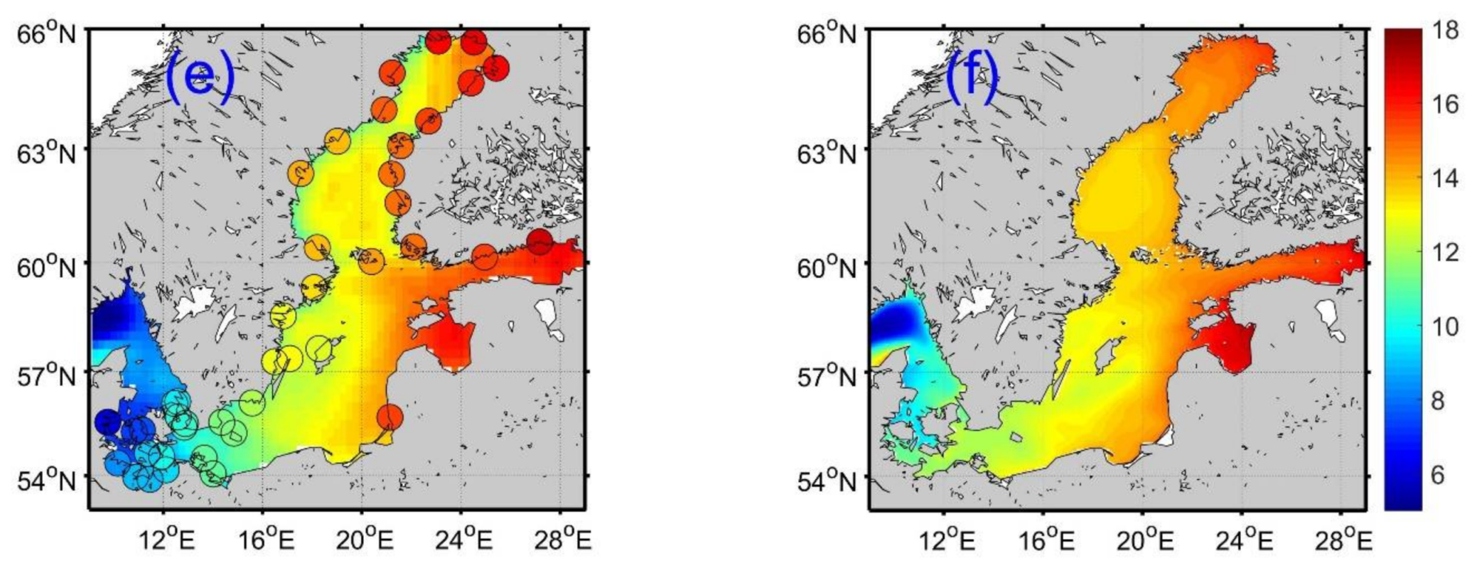
Figure 2e,f show the distribution of standard deviation (STD) of altimetry and SMHI data, respectively. Compared with the overlaid STD of tide gauge data (13–18 cm), altimetry data present slightly lower STD along the coasts of the Baltic Sea. SMHI reanalysis shows a similar spatial pattern of STD as altimetry data, e.g., STD increases from ~11 cm at the entrance to ~17 cm in the interior and in the gulfs of the Baltic Sea. In the coastal regions, higher STD is present in the SMHI data, which fits the tide gauge data better than the altimetry data.
3. Method
The method for computing CSEOFs is based on the theory of harmonizable cyclostationary functions, with CSEOFs defined as products of the Bloch and Fourier functions [25]. The CSEOF method decomposes space-time data (T) into a series of modes comprised of a spatial component (LV), and a corresponding temporal principle component time series (PCTS). The system is described as
where T(r, t) is space-time data, LV is composed of spatial patterns representing a physical process modulated by a stochastic time series PC.
Based on this formulation, the main difference between CSEOFs and the more widely used empirical orthogonal function (EOF) analysis is that CSEOF spatial patterns (LVs) are allowed to vary in time with a “nested period” that is selected a priori. In other words, each LV is a set of spatial patterns that repeat with the nested period over the length of the dataset, and the amplitude of the periodic LV is modulated by the PCTS. For monthly data and a one-year nested period, for example, each mode is composed of twelve sequential spatial patterns (the LV) and one PCTS. This allows the CSEOF decomposition to capture the temporal evolution of a physical process (i.e., the annual sea level cycle) in the LV, while the corresponding PCTS explains the amplitude of this physical process through time, i.e., the interannual variability of the annual sea level cycle. The nested period of the CSEOF analysis is generally selected based on some physical understanding or intuition regarding the data to be studied. When studying the annual cycle known to be present in many geophysical datasets, for instance, a nested period of one year is chosen. The resulting LV would contain a spatial pattern for each month and would describe the physical evolution of the annual cycle through the year. The PCTS then describes the amplitude change—or strength—of the annual cycle from year to year. Further details of this technique can be found in Kim et al. (2015).
4. Results
4.1. Temporal and Spatial Variability of the Annual Sea Level Cycle
Figure 3 shows the mean seasonal sea level cycle (mm, e.g., average of each calendar month) during 1993–2014 at the selected 42 tide gauges. Despite the large geophysical distance between the stations, most of the records show a well-defined minimum sea level in Spring (April–May) and a relatively broad maximum sea level in winter (December–February) [11]. The patterns of the seasonal cycle are slightly asymmetric and similar at all the selected tide gauges but different from each other on the maximum (varies from 0 to 100 mm) and minimum (varies from −150 mm to −40 mm) seasonal cycle amplitudes. The magnitude and time of the maximum and minimum values relate to the latitude of the stations (e.g., at the entrance and inside of the Baltic Sea) and regional atmospheric conditions [14]. Several stations located at the entrance of the Baltic Sea (e.g., Danish Straits) show maximum sea level in autumn, which may also relate to local ocean dynamic conditions [26].
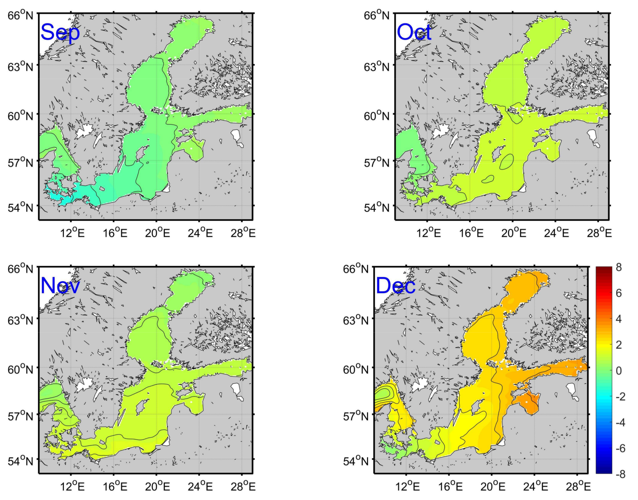
In order to capture the time-varying spatial pattern and temporal variation of the annual sea level cycle, the CSEOF analysis is applied to satellite altimetry, tide gauge data, and SMHI reanalysis, respectively. Figure 4 shows the first mode of CSEOF computed from altimetry data over the time period 1993–2014. It captures the spatial variation of the annual cycle and accounts for 33% of the sea level variability. In Figure 4, the spatial patterns (LVs, color images) denote monthly variations of the annual sea level cycle. The PC time series are normalized (dimensionless) by its mean and denotes the interannual variations of the LVs. Recombining the LVs and PC using Equation (1) produces the contribution of the annual cycle to regional sea level over the length of the record.
In Figure 4, the locations with less than 100% of altimetry data available are removed. It is seen that coherent positive annual sea-level variations dominate the Baltic Sea in December to March. The highest annual signal is observed in January in the eastern Baltic Sea and gulfs. The magnitude of the annual cycle decreases from west to east in February–March and changes to a negative phase in May–August. Moreover, the annual signal variations are more significant in the Baltic Sea than in the entrance of the Baltic Sea.
The same procedure is applied on the 32 tide gauge data (199–2014) and the results are overlaid in Figure 4. Similar to that of the altimetry data, the first CSEOF mode of the tide gauge data accounts for 33% of sea level variability. The annual cycle is also in the tide gauge data peaking during the winter (December to February). Also, the sites in the Baltic Sea show coherent and stronger annual sea level cycle than those in the entrance of the Baltic Sea, where the annual sea level cycle is affected by non-atmospheric factors due to active water exchange in the regions. In Figure 4, consistent annual sea level variations are observed between tide gauge and altimetry data in the Baltic Sea. Compared with the altimetry data, the tide gauge data exhibits stronger annual sea level variations in winter, particularly in the Gulf of Bothnia. Lower variations are observed in the entrance of the Baltic Sea in December and January. The PC time series of the first CSEOF mode (Figure 4) indicate that the interannual variability of the annual sea level is similar in the altimetry and tide gauge data sets, e.g., low and high peaks in 1996/2010 and 2008/2012, respectively. Figure 4 also show that the difference between the tide gauge and the satellite altimetry data derived annual cycle is more significant during the winter than in other seasons. This cannot be shown by applying a least squares adjustment to the data sets.
In Figure 5, we present the monthly LVs (color images) estimated from the SMHI reanalysis (Figure 4b). Compared with Figure 4, higher and lower annual sea level variations are observed from the SMHI reanalysis in February–May and October–December, respectively. The overlaid PC time series in Figure 4 demonstrates weaker interannual variation in SMHI data (e.g., 2008/2012). Furthermore, the maximum annual sea level cycle in the Gulf of Bothnia and the Gulf of Finland have a 1-month lag (in February) in the SMHI datasets (Figure 4b). In short, while model reanalysis may simulate the magnitude of the annual sea level cycle well (accounts for 40% of sea level variability), it underestimates the interannual variability of the signal.
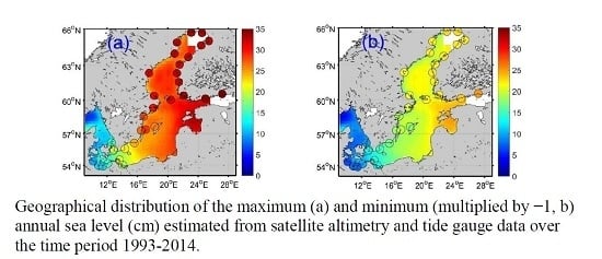
4.2. Extreme Annual Sea Level Cycle
The south-western coasts (the Bay of Mecklenburg) and the eastern coasts (the Gulf of Riga with Pärnu Bay, the Gulf of Finland, the northern part of the Gulf of Bothnia) are particularly exposed to extreme sea levels. The significant fluctuations of the annual sea level superimposed on the local sea level variations on short time scales (i.e., storm surges) could increase or decrease the flooding risks over these regions.
Figure 6 shows the maximum (left panels) and minimum (right panels) annual sea level amplitude calculated from the first CSEOF mode of altimeter data (Figure 6a,b) and SMHI reanalysis (Figure 6c,d) over the time period 1993–2014 (Equation (1)). The minimum annual sea level amplitude is multiplied by −1 for illustration purposes. The maximum annual sea level amplitude (Figure 6a or Figure 6c) is highly consistent with the distributions of extreme (maximum and minimum) sea levels indicated by the observed water levels, with amplitudes of the observed extreme sea levels at the gauge stations in [27].
In Figure 6a,b, the maximum and minimum annual sea level amplitudes gradually increase from the western to eastern coast of the Baltic Sea and the maximum amplitude exceeds 30 cm in the gulfs. Compared with tide gauge data, satellite altimetry indicates lower extreme values in the coastal regions of the Baltic sea of the same magnitude as at the Baltic entrance. SMHI analysis (Figure 6c,d) also demonstrates a gradual increase from the entrance to the heads of the gulfs. Compared with Figure 6a, the SMHI reanalysis (Figure 6c) underestimates the maximum annual sea level and might therefore underestimate the flooding risk in the study period. By comparing Figure 6b with Figure 6d, it is noted that the SMHI reanalysis overestimates the minimum annual sea level (Figure 6d) and therefore amplifies the flooding risk in the altimetry era.
4.3. Relations between Annual Sea Level and Atmospheric Parameters
4.3.1. Wind Speed
The Baltic Sea is strongly exposed to the influence of the North Atlantic atmospheric circulation. This implies that the long-term behavior of regional sea level variability is significantly influenced by large-scale wind and air pressure fields [28,29]. Here, we discuss the spatial patterns and temporal fluctuations of the annual zonal wind cycle.
Figure 7 shows the 12 LVs of zonal wind speed from 20CR2 (20th Century Reanalysis V2, [30]) datasets and the PC time series for the period 1993–2012. High positive and negative annual zonal wind speed variations are observed over the southern Baltic Sea during the winter and the Spring, respectively, which may cause the redistribution of water and contribute to the spatial patterns of the annual sea level cycle (Figure 4). In the lower part of Figure 7, the fluctuations of the annual zonal wind speed (e.g., PC time series of the CSEOF first mode) are overlaid with the annual sea level variations. The correlation coefficient of 0.7 ± 0.1 (at 95% confidence level) between the PC time series indicates a significant contribution from zonal annual wind speed on interannual variations of the annual sea level cycle in the period 1993–2012. Moreover, there is no phase difference in the maximum cross correlation between the time series, which indicates a direct effect of zonal wind speed on the annual sea level variability.
4.3.2. NAO Index
The NAO is a major atmospheric, basin scale climate pattern. It dominates atmospheric variability over the North Atlantic and Europe. Previous studies show that the variability of tide gauge sea level in the Baltic Sea is highly correlated with the NAO index at the annual and interannual time scales, especially during the winter. Stramska and Chudziak [31] also reported high correlation between winter NAO [32] and winter averaged SLA derived from altimetry.
In order to study similarities between monthly NAO index and the annual sea level cycle variability, the 13-month running mean of the station-based NAO index [32] was included in the lower panel of Figure 4. In 1996/2010 and 2012, the negative/positive phase of the NAO corresponded to significant drops in the annual sea level amplitude. Similar CC of 0.4 ± 0.1 (at 95% confidence level) is shown between the NAO index and all datasets with a one-month phase lag in the maximum cross correlation. The results imply that the fluctuations of the annual sea level cycle are significantly correlated with the NAO index over 1993–2014.
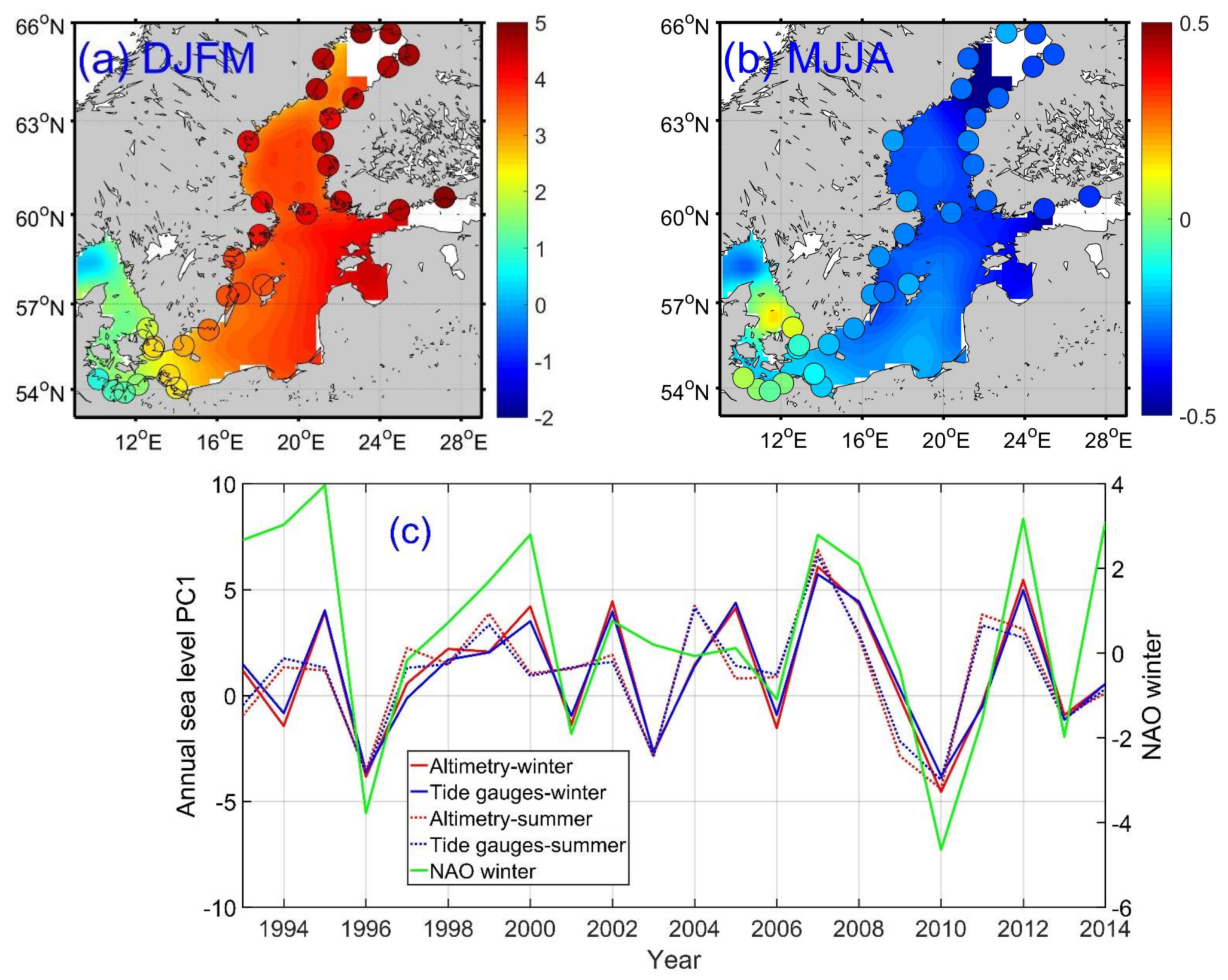
Figure 8a,b show the average variations of the annual sea level cycle during the winter months (December–February) and the spring-summer months (May–August) derived from the LVs for the first CSEOF mode, respectively. In Figure 8a, tide gauge data show the consistent positive annual sea level cycle as altimetry data in the coastal regions of the Baltic Sea. In summer (Figure 8b), consistent negative annual sea level cycles are presented from the tide gauge and altimetry data. Figure 8c denotes the seasonal averaged PC time series and consistent temporal variations of the annual sea level cycle from the tide gauge and altimetry data. Figure 8c shows a correlation coefficient of 0.8 ± 0.2 (at 95% confidence level), which confirms the strong relations between interannual variations of the annual sea level cycle and the winter NAO [32], particularly in 1996 and 2010.
4.3.3. Sea Level Pressure
The NAO-index used in this study is calculated from station-based sea level pressure (SLP) measurements. The SLP difference between the Baltic Sea and the North Atlantic also affects the sea level in the Baltic Sea. As a general rule, the drop of atmospheric pressure at sea level in 1 hPa results in a 1 cm increase in sea level. Extreme water levels in the Baltic Sea are related to sudden storm events caused by deep low-pressure phenomena [27]. Herein we perform a CSEOF analysis to the monthly SLP from NCEP/NCAR Reanalysis Products [33] to investigate the effects of the spatial and temporal variations of the annual SLP on annual sea level variability during 1993–2014.
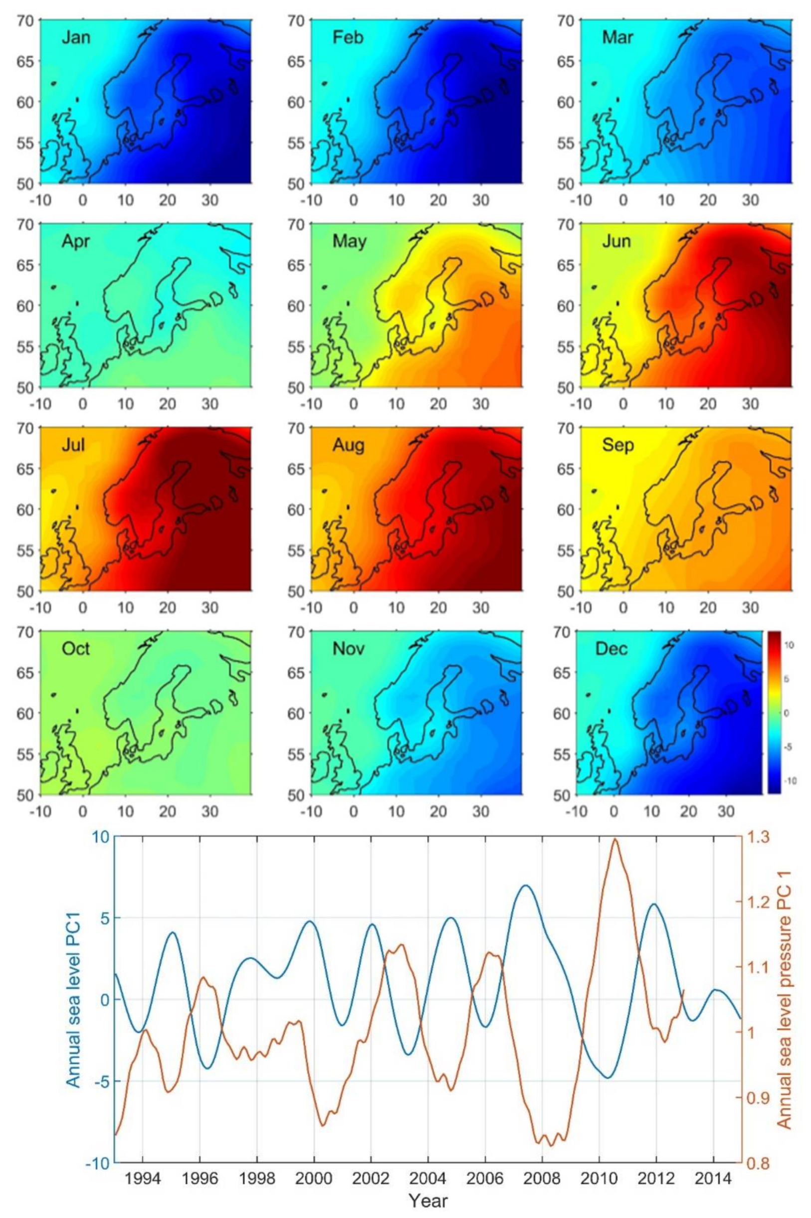
The color images in Figure 9 show the spatial pattern of CSEOF analyzed using the annual SLP cycle (the first mode). During the winter, the negative annual SLP cycle dominates the Northern Atlantic Ocean, which is consistent with the positive pattern of the annual sea level variation observed in the Baltic Sea (Figure 4). As a consequence of the SLP pattern over the Baltic Sea, the influence of the SLP on the annual sea level variations is stronger in the northern Baltic Sea than in the southern region. During the summer, the annual SLP cycle shifts from a negative to a positive phase in the North Atlantic Ocean. Similarly, the pattern of annual sea level cycle in Figure 4 is coherent with the positive SLP annual cycle pattern (Figure 9a) between May and July.
Figure 9 also shows SLA and SLP PC time series of the first CSEOF mode (standardized by the mean of the PC time series) over the study area in Figure 1. The CC of 0.4 ± 0.1 (at 95% confidence level) is observed between the time series in the period of 1993–2013. The CC increases to 0.6 ± 0.1 (at 95% confidence level) if the data before 1995 are excluded in the computation. The significant drops of SLA in 1996 and 2010 correspond to the SLP variation over the same time period. Following the fall of annual sea level amplitude in 2010, a significant rise in annual sea level amplitude in 2011 is coherent with the annual SLP increase in the same year. The temporal variability of SLP suggests that the variability of annual sea level is in part due to an isostatic response of the sea level to air pressure changes in the selected time period.
4.3.4. Air Temperature
The sea level can be affected by temperature due to the thermal expansion of the water column. At long time scales, air temperature should be closely coupled to water temperature [10]. Lehmann et al. [21] assessed the climate variability in the Baltic Sea for the period 1958–2009 and concluded that the recent changes in the warming trend in the Baltic Sea are associated with changes in large-scale atmospheric circulation over the North Atlantic.
Here, we performed CSEOF analysis to the 20CR2 air-temperature data (in degree K, [30]) in the Baltic Sea over 1993–2012 to study its correlation with the annual sea level variability. The spatial distributions of 12 LVs (Figure 10) demonstrate negative annual air temperature variation in winter and positive variation in summer. The PC time series (over the regions in Figure 1) of the annual air temperature cycle is overlaid with that of the annual sea level cycle in the lower panel of Figure 10. Coherent annual cycle fluctuations between air temperature and SLA are observed, except in 2001. The CC of −0.6 ± 0.1 (at 95% confidence level) is obtained in the time span 1993–2012, implying that the fluctuations of the annual air temperature cycle are also linked to the annual sea level fluctuation (e.g., 1995–1996, 2008 and 2010).
5. Discussion
In the present study, we have analyzed DUACS global sea level products to investigate the spatio-temporal annual sea level variability in the Baltic Sea. The global sea level products show RMSd of 1-8 cm and high correlations (>0.9) against tide gauge data in the Baltic Sea. New regional altimetry sea level products are required to better describe the sea level variability in the near future [34].
Passaro et al. [26] used the ALES (Adaptive Leading Edge Subwaveform Retracker) data set and the reference ESA Sea Level Climate Change Initiative data to study the annual sea level cycle in the North Sea-Baltic Sea transition area (2002–2010). In their study, the spatial patterns and temporal variations of the annual sea level (Figure 4) and zonal wind (Figure 7) in the entrance of the Baltic Sea indicate that wind stress is the dominating driver of the annual cycle variations in the region. The results using the CSEOF methods (Figure 7) supports these finding. With a view to the influence of SLP, the Baltic Sea is located closer to the sea level pressure center in the North Atlantic Ocean than the entrance of the Baltic Sea (Figure 9). This may explain why SLP contributes more to the annual sea level cycle variations in this region compared to at the entrance. This is also in agreement with the findings in [14], which focus on local sea level variability.
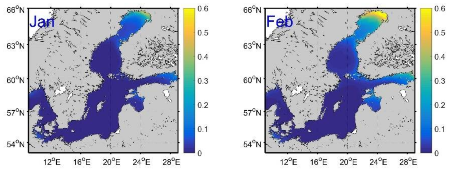
In Figure 4, the CSEOF analysis of altimetry data is not available in the head of Gulf of Bothnia and the Gulf of Finland. The lack of data is attributed to ice-coverage in December to May (Figure 11). In the Gulf of Bothnia, the sea ice thickness computed from the SMHI reanalysis exceeds 0.6 m in the period of February to March (Figure 11), which explains the observed low annual sea level pattern at the edges of the sea ice (February and March in Figure 4). The decrease of the annual sea level is not significant in the Gulf of Finland, which may be attributed to thinner and smaller coverage of sea ice in the regions.
For the tide gauge data not included in Figure 4, we have conducted an analysis of the periods covered with observations. Figure 12a,b show the annual sea level cycle determined from the three datasets using the CSEOF method at Skagsudde (1994–2014) and Klaipeda (1993–2011), respectively. Overall, altimetry data capture the peaks of the annual sea level, while the SMHI data overestimate and underestimate the negative and positive peaks, respectively, of annual sea level at Skagsudde. At Klaipeda (in the Gulf of Gdansk), SMHI reanalysis shows better agreement with the tide gauge data than altimetry data. Klaipeda is located inside the lagoon and as a result, the coastline affects the altimetry data. SMHI reanalysis includes the effects of river runoff in the model, implying that the SMHI data are more accurate than altimetry data in these coastal regions. In other southeastern regions of the Baltic Sea, e.g., the Gulf of Riga, there is a lack of in-situ measurements for validation.
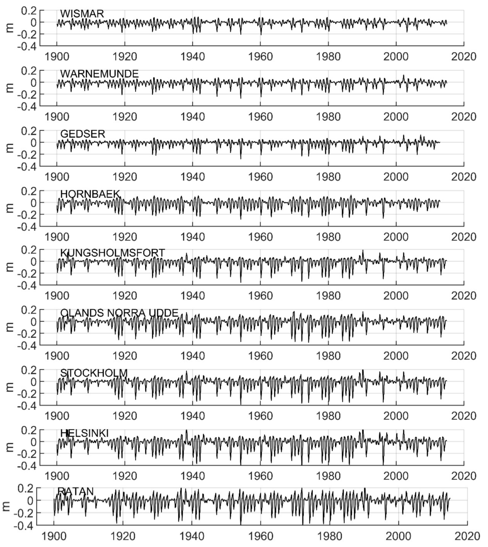
In order to further test the performance of the CSEOF method in capturing the regional annual sea level variability, we carry out the analysis on the same tide gauge data (Table 1) in [14] for 1900–2012 time period (Figure 13). The mean of the data records is removed and the inverted barometer (IB) correction is not applied. Consistent temporal variations of the annual sea level are obtained when using continuous or discrete wavelet analysis (DWT) [14] and the CSEOF method. For example, considerable changes in the periods around 1920, 1930, 1955 and 197–1990 (with some interruption between 1975 and 1978) are observed. Both methods illustrate a weak seasonal cycle (especially in the 1940s and 1990s to 2000s). Furthermore, the coherent variability increases from South (Wismar) to North (Ratan) in the Baltic Sea, which agree with the findings from the period 1993–2014.
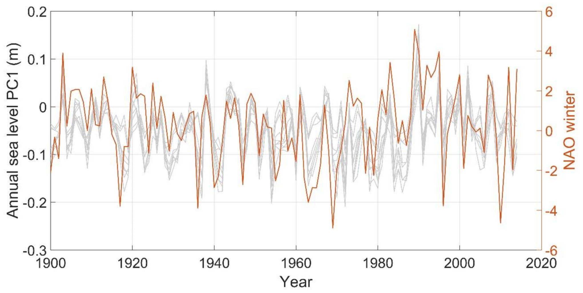
We further investigate the relations between the atmospheric parameters and the annual sea level variations using CSEOF analysis for the period 1900–2012. The annual sea level PC time series show high correlation with zonal wind PC (Figure 14, not standardized). This is consistent with the proposed high contributions of zonal wind to the annual sea level cycle in previous studies. Moreover, we found the winter NAO is also highly correlated with the variations of the annual sea level cycle (Figure 15). On the other hand, the parameters are not independent with each other. In 1990, both zonal wind and winter NAO contributed to the high annual sea level cycle. Table 2 lists the correlations between tide gauge PC time series and the parameters. In contrast to the period 1993–2014, the high correlations between air temperature/NAO and the tide gauge annual sea level cycle variations are not identified in 1900–2012.
6. Conclusions
In this work, through a combined analysis of tide gauge data, satellite altimetry, and regional model analysis, we have investigated the annual sea level fluctuation in the semi-enclosed Baltic Sea, which has widely been considered to be fairly constant in time. The CSEOF method is adopted to examine the interannual variations of the annual sea level cycle. All the datasets show coherent spatial and temporal annual sea level cycle variability in the Baltic Sea. The positive/negative annual sea level variations are observed in December-February/May-July in all tide gauge records and altimetry data. Tide gauge show higher annual sea level variation than altimetry data during the winter. SMHI reanalysis have a 1-month lag in the maximum annual the maximum annual sea level cycle. The maximum and minimum annual sea levels computed from the first mode of CSEOF analyzed altimetry data and SMHI reanalysis underestimate the flooding risk, particularly in the high flooding risky regions due to storm surges (e.g., the Gulf of Finland and the Gulf of Bothnia). In the Gulf of Gdansk and the Gulf of Riga, the model reanalysis is valuable for estimating the flooding risk over the region lack of tide gauge data.
Possible atmospheric forcing factors associated with the annual sea level variability are investigated. In the southern Baltic Ocean, strong positive and negative annual zonal winds are shown during the winter and summer, respectively. The zonal winds contribute directly to the coherent annual sea level cycle variations in the Baltic Sea. In the period 1993–2014, the NAO-index shows a coefficient of correlation 0.4 ± 0.1 with all the three datasets derived variations of the annual sea level cycle. In the winter, higher coherence (CC of 0.8 ± 0.2) is observed between averaged annual LVs and winter NAO. Moreover, the annual air pressure variations in the Northern Atlantic Ocean are also correlated with spatial and temporal annual sea level cycle variations, particularly in 1996 and 2010. The air temperature also contributes to the annual sea level variations, especially in 2008/2010. For a longer time period (1900–2012), the zonal wind and winter NAO are highly correlated with the variations of annual sea level cycle. However, the high correlations between air temperature/SLP/NAO and annual sea level variations are not significant. Changes in atmospheric forcing might cause the identified variations of the correlations in the altimetry era.
Acknowledgments
This work was supported by the National Key Project of Research and Development Plan of China (Grant No. 2016YFC1401905), and the open research fund of the Jiangsu Key Laboratory of Coast Ocean Resources Development and Environment Security (Hohai University, grant JSCE201502). The tide gauge data are provided by the PSMSL (Permanent Service for Mean Sea Level). We are grateful to the AVISO (Archiving, Validation and Interpretation of Satellite Oceanographic data, www.aviso.oceanobs.com) for providing the satellite altimeter and DAC (dynamic atmospheric correction) data. The 20CR2 and NCEP/NCAR data are available at http://www.esrl.noaa.gov/psd/data/gridded/. The SMHI dataset are available at CMEMS http://marine.copernicus.eu/. We thank the anonymous reviewers for their constructive comments, which have provided many valuable improvements to the article. The views, opinions, and findings contained in this report are those of the authors and should not be construed as an official NOAA or U.S. Government position, policy, or decision.
Author Contributions
Y.C. conceived and designed the experiments; Y.C. and Q.X. analyzed the data; Y.C. wrote the paper; Q.X. and X.L. critically revised the paper.
Conflicts of Interest
The authors declare no conflict of interest.
Appendix A
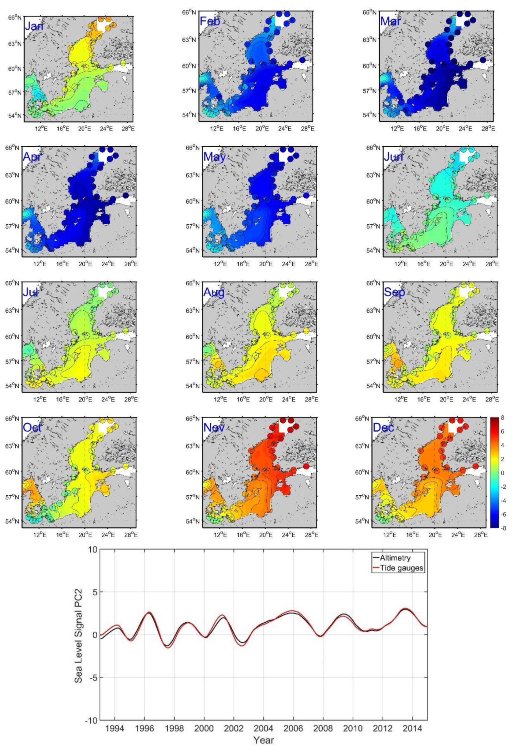
The CSEOF second mode related to longer sea level variability (>3 years) in the region. It accounts for 24%, 23%, and 23% of altimetry, tide gauge and SMHI reanalysis sea level variability, respectively. The color images in Figure A1 show the spatial patterns of the signal from January to December (cm). The signal increases from the entrance to interior of Baltic Sea. Low and high variability presented in spring (February–May) and winter (November–December) and to reach maximum/minimum in November/March, respectively. Tide gauge data show weaker variability than altimetry data in summer. The time series implies consistent sea level variability between tide gauge and altimetry data in the Baltic Sea.
Figure A1.
CSEOF second mode captures the spatial patterns (color images) and temporal variations (time series) of long-term sea level cycle: monthly time-dependent LVs (cm, January thru December) computed from satellite altimetry and tide gauge data and the PC time series (PC2, dimensionless) of altimetry data and tide gauge data for 1993–2014. For each dataset, the PCs are normalized with mean PC2 time series and the LVs are times by mean of PC2 time series.
References
- Jaagus, J.; Suursaar, Ü. Long-term storminess and sea level variations on the estonian coast of the Baltic Sea in relation to large-scale atmospheric circulation. Estonian J. Earth Sci. 2013, 62, 73–92. [Google Scholar] [CrossRef]
- Madsen, K.S.; Høyer, J.L.; Fu, W.; Donlon, C. Blending of satellite and tide gauge sea level observations and its assimilation in a storm surge model of the North Sea and Baltic Sea. J. Geophys. Res. Oceans 2015, 120, 6405–6418. [Google Scholar] [CrossRef]
- Xu, Q.; Cheng, Y.; Plag, H.-P.; Zhang, B. Investigation of sea level variability in the Baltic Sea from tide gauge, satellite altimeter data, and model reanalysis. Int. J. Remote Sens. 2015, 36, 2548–2568. [Google Scholar] [CrossRef]
- Cheng, Y.; Andersen, O.B.; Knudsen, P.; Xu, Q. Multimission Satellite Altimetric Data Validation in the Baltic Sea. In Proceedings of the 2014 IEEE Geoscience and Remote Sensing Symposium, Quebec City, QC, Canada, 13–18 July 2014; pp. 4536–4539. [Google Scholar]
- Han, G.; Loder, J.; Petrie, B. Tidal and non-tidal sea level variability along the coastal nova scotia from satellite altimetry. Int. J. Remote Sens. 2010, 31, 4791–4806. [Google Scholar] [CrossRef]
- Han, G. Sea level and surface current variability in the Gulf of St Lawrence from satellite altimetry. Int. J. Remote Sens. 2004, 25, 5069–5088. [Google Scholar] [CrossRef]
- Feng, X.; Tsimplis, M.N.; Marcos, M.; Calafat, F.M.; Zheng, J.; Jordà, G.; Cipollini, P. Spatial and temporal variations of the seasonal sea level cycle in the Northwest Pacific. J. Geophys. Res. Oceans 2015, 120, 7091–7112. [Google Scholar] [CrossRef]
- Handoko, E.; Fernandes, M.; Lázaro, C. Assessment of altimetric range and geophysical corrections and mean sea surface models—Impacts on sea level variability around the Indonesian seas. Remote Sens. 2017, 9, 102. [Google Scholar] [CrossRef]
- Bosch, W.; Dettmering, D.; Schwatke, C. Multi-mission cross-calibration of satellite altimeters: Constructing a long-term data record for global and regional sea level change studies. Remote Sens. 2014, 6, 2255–2281. [Google Scholar] [CrossRef]
- Hünicke, B.; Zorita, E. Trends in the amplitude of Baltic Sea level annual cycle. Tellus A 2008, 60, 154–164. [Google Scholar] [CrossRef]
- Stramska, M.; Kowalewska-Kalkowska, H.; Świrgoń, M. Seasonal variability in the Baltic Sea level. Oceanologia 2013, 55, 787–807. [Google Scholar] [CrossRef]
- Etcheverry, L.R.; Saraceno, M.; Piola, A.R.; Valladeau, G.; Möller, O. A comparison of the annual cycle of sea level in coastal areas from gridded satellite altimetry and tide gauges. Cont. Shelf Res. 2015, 92, 87–97. [Google Scholar] [CrossRef]
- Medvedev, I. Seasonal fluctuations of the Baltic Sea level. Russ. Meteorol. Hydrol. 2014, 39, 814–822. [Google Scholar] [CrossRef]
- Barbosa, S.M.; Donner, R.V. Long-term changes in the seasonality of Baltic Sea level. Tellus A 2016, 68, 30540. [Google Scholar] [CrossRef]
- Cheng, Y.; Hamlington, B.; Plag, H.-P.; Xu, Q. Influence of enso on the variation of annual sea level cycle in the south china sea. Ocean Eng. 2016, 126, 343–352. [Google Scholar] [CrossRef]
- Cheng, Y.; Plag, H.-P.; Hamlington, B.D.; Xu, Q.; He, Y. Regional sea level variability in the bohai sea, yellow sea, and east china sea. Cont. Shelf Res. 2015, 111, 95–107. [Google Scholar] [CrossRef]
- Kim, K.-Y.; Wu, Q. A comparison study of eof techniques: Analysis of nonstationary data with periodic statistics. J. Clim. 1999, 12, 185–199. [Google Scholar] [CrossRef]
- Hamlington, B.; Leben, R.; Nerem, R.; Kim, K.-Y. The effect of signal-to-noise ratio on the study of sea level trends. J. Clim. 2011, 24, 1396–1408. [Google Scholar] [CrossRef]
- Kim, K.-Y.; Hamlington, B.; Na, H. Theoretical foundation of cyclostationary eof analysis for geophysical and climatic variables: Concepts and examples. Earth Sci. Rev. 2015, 150, 201–218. [Google Scholar] [CrossRef]
- Høyer, J.L.; Karagali, I. Sea surface temperature climate data record for the North Sea and Baltic Sea. J. Clim. 2016, 29, 2529–2541. [Google Scholar] [CrossRef]
- Lehmann, A.; Getzlaff, K.; Harlaß, J. Detailed assessment of climate variability of the Baltic Sea area for the period 1958–2009. Clim. Res. 2011, 46, 185–196. [Google Scholar] [CrossRef]
- Rio, M.H.; Pascual, A.; Poulain, P.M.; Menna, M.; Barceló, B.; Tintoré, J. Computation of a new mean dynamic topography for the mediterranean sea from model outputs, altimeter measurements and oceanographic in-situ data. Ocean Sci. Discuss. 2014, 11, 655–692. [Google Scholar] [CrossRef]
- Cheng, X.; McCreary, J.P.; Qiu, B.; Qi, Y.; Du, Y. Intraseasonal-to-semiannual variability of sea-surface height in the astern, equatorial Indian Ocean and southern bay of bengal. J. Geophys. Res. Oceans 2017, 122, 4051–4067. [Google Scholar] [CrossRef]
- Holgate, S.J.; Matthews, A.; Woodworth, P.L.; Rickards, L.J.; Tamisiea, M.E.; Bradshaw, E.; Foden, P.R.; Gordon, K.M.; Jevrejeva, S.; Pugh, J. New data systems and products at the permanent service for mean sea level. J. Coast. Res. 2013, 29, 493–504. [Google Scholar] [CrossRef]
- Kim, K.-Y.; North, G.R. Eofs of harmonizable cyclostationary processes. J. Atmos. Sci. 1997, 54, 2416–2427. [Google Scholar] [CrossRef]
- Passaro, M.; Cipollini, P.; Benveniste, J. Annual sea level variability of the coastal ocean: The Baltic Sea-North Sea transition zone. J. Geophys. Res. Oceans 2015, 120, 3061–3078. [Google Scholar] [CrossRef]
- Wolski, T.; Wiśniewski, B.; Giza, A.; Kowalewska-Kalkowska, H.; Boman, H.; Grabbi-Kaiv, S.; Hammarklint, T.; Holfort, J.; Lydeikaitė, Ž. Extreme sea levels at selected stations on the Baltic Sea coast. Oceanologia 2014, 56, 259–290. [Google Scholar] [CrossRef]
- Andersson, H.C. Influence of long-term regional and large-scale atmospheric circulation on the Baltic Sea level. Tellus A 2002, 54, 76–88. [Google Scholar] [CrossRef]
- Jevrejeva, S.; Moore, J.; Woodworth, P.; Grinsted, A. Influence of large-scale atmospheric circulation on European Sea level: Results based on the wavelet transform method. Tellus A 2005, 57, 183–193. [Google Scholar] [CrossRef]
- Compo, G.P.; Whitaker, J.S.; Sardeshmukh, P.D.; Matsui, N.; Allan, R.J.; Yin, X.; Gleason, B.E.; Vose, R.S.; Rutledge, G.; Bessemoulin, P.; et al. The twentieth century reanalysis project. Q. J. R. Meteorol. Soc. 2011, 137, 1–28. [Google Scholar] [CrossRef]
- Stramska, M.; Chudziak, N. Recent multiyear trends in the Baltic Sea level. Oceanologia 2013, 55, 319–337. [Google Scholar] [CrossRef]
- Hurrell, J.W. Decadal trends in the north atlantic oscillation: Regional temperatures and precipitation. Science 1995, 269, 676–679. [Google Scholar] [CrossRef] [PubMed]
- Kalnay, E.; Kanamitsu, M.; Kistler, R.; Collins, W.; Deaven, D.; Gandin, L.; Iredell, M.; Saha, S.; White, G.; Woollen, J. The NCEP/NCAR 40-year reanalysis project. Bull. Am. Meteorol. Soc. 1996, 77, 437–471. [Google Scholar] [CrossRef]
- Cipollini, P.; Calafat, F.M.; Jevrejeva, S.; Melet, A.; Prandi, P. Monitoring sea level in the coastal zone with satellite altimetry and tide gauges. Surv. Geophys. 2017, 38, 33–57. [Google Scholar] [CrossRef]
Figure 1.
Map of the study area with bathymetry of 50 m overlaid. Locations of 42 selected tide gauges are shown as blue filled dots with their according numbers presented in Table 1. The zoom in region is the entrance of Baltic Sea. DK: Denmark, AL: Aland.
Figure 1.
Map of the study area with bathymetry of 50 m overlaid. Locations of 42 selected tide gauges are shown as blue filled dots with their according numbers presented in Table 1. The zoom in region is the entrance of Baltic Sea. DK: Denmark, AL: Aland.
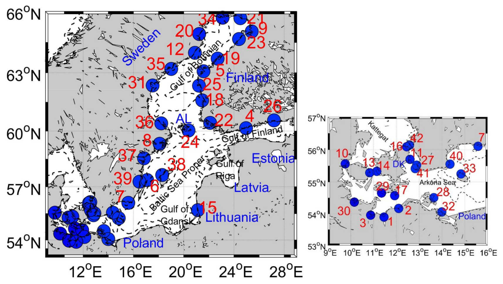
Figure 2.
Geographical distribution of Root Mean Square difference (a,b cm) and correlation coefficient (c,d) between tide gauge data, altimetry data (a,c) and the Swedish Meteorological and Hydrological Institute (SMHI) reanalysis (b,d), and standard deviation (cm) of tide gauge data/altimetry data (e) and SMHI reanalysis (f) for the time span of 1993–2014.
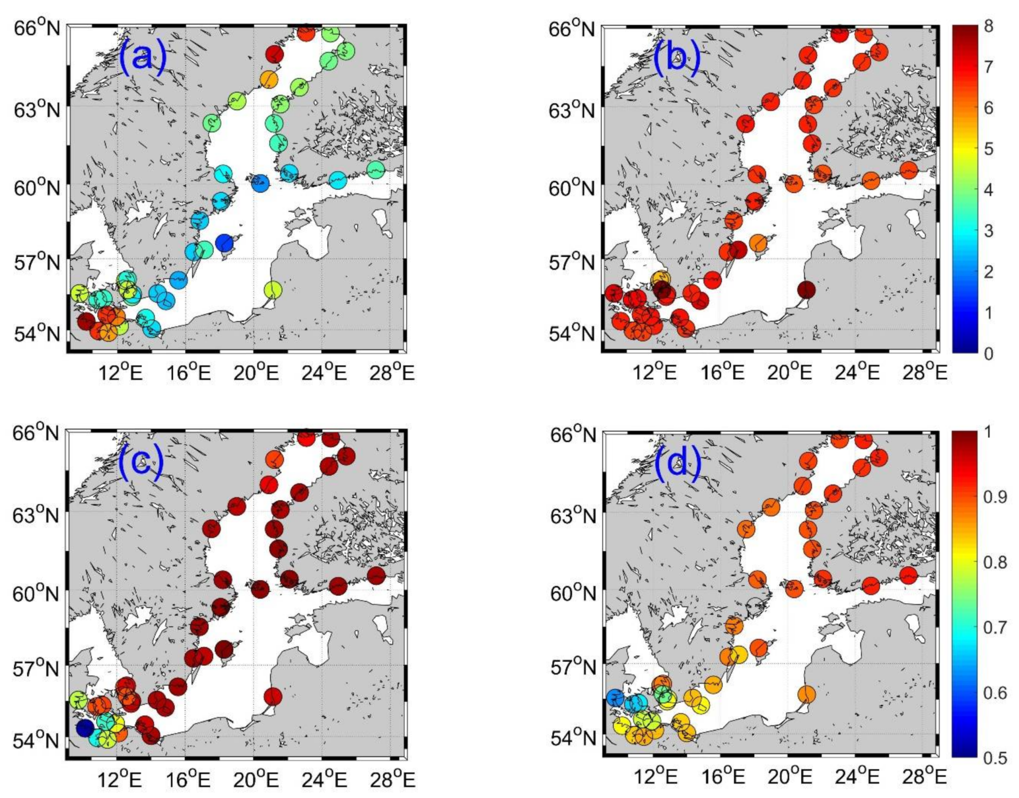

Figure 3.
Mean sea level (m) calculated at the selected 42 stations over the time period 1993–2014 in the Baltic Sea.
Figure 3.
Mean sea level (m) calculated at the selected 42 stations over the time period 1993–2014 in the Baltic Sea.
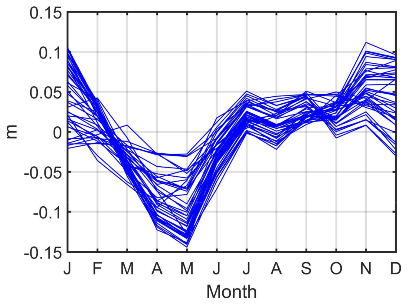
Figure 4.
The first cyclostationary empirical orthogonal function (CSEOF) mode captures the spatial patterns (color images) and temporal variations (time series) of the annual sea level cycle: monthly time-dependent loading vectors (LVs) (cm, January to December) computed from satellite altimetry and tide gauge data and the principal component (PC) time series (PC1, dimensionless) of altimetry data (black line), tide gauge data (blue line) and SMHI model reanalysis (gray line) for 1993–2014. The 13-month running mean filtered station-based North Atlantic Oscillation (NAO) index (red line) is overlaid. Each PC is normalized by its mean value and the LV is multiplied by the value.
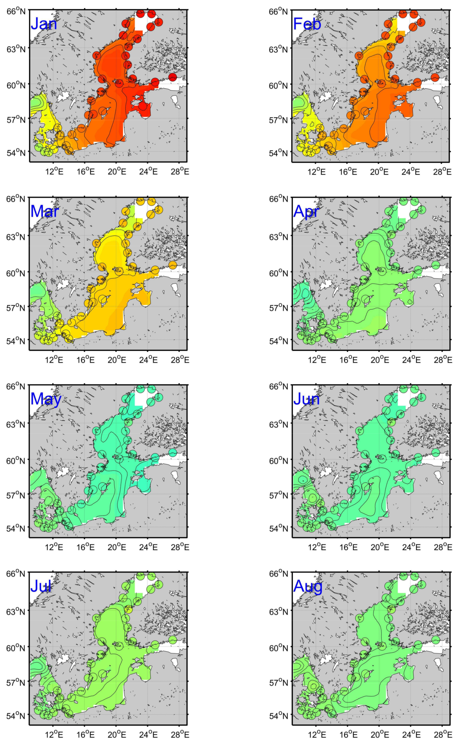
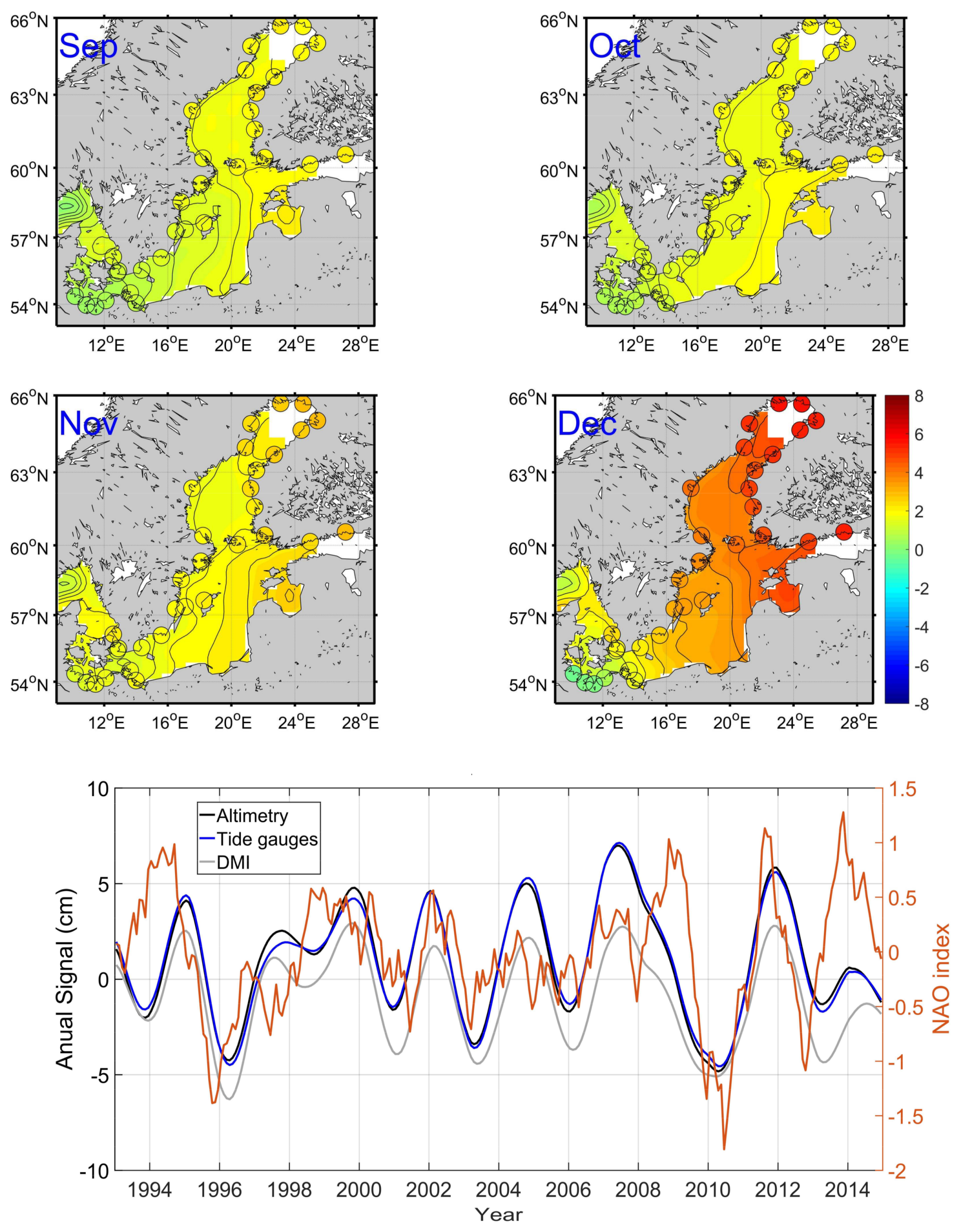
Figure 5.
Similar to Figure 4 but for SMHI reanalysis of CSEOF first mode monthly time-dependent LVs (cm).
Figure 5.
Similar to Figure 4 but for SMHI reanalysis of CSEOF first mode monthly time-dependent LVs (cm).
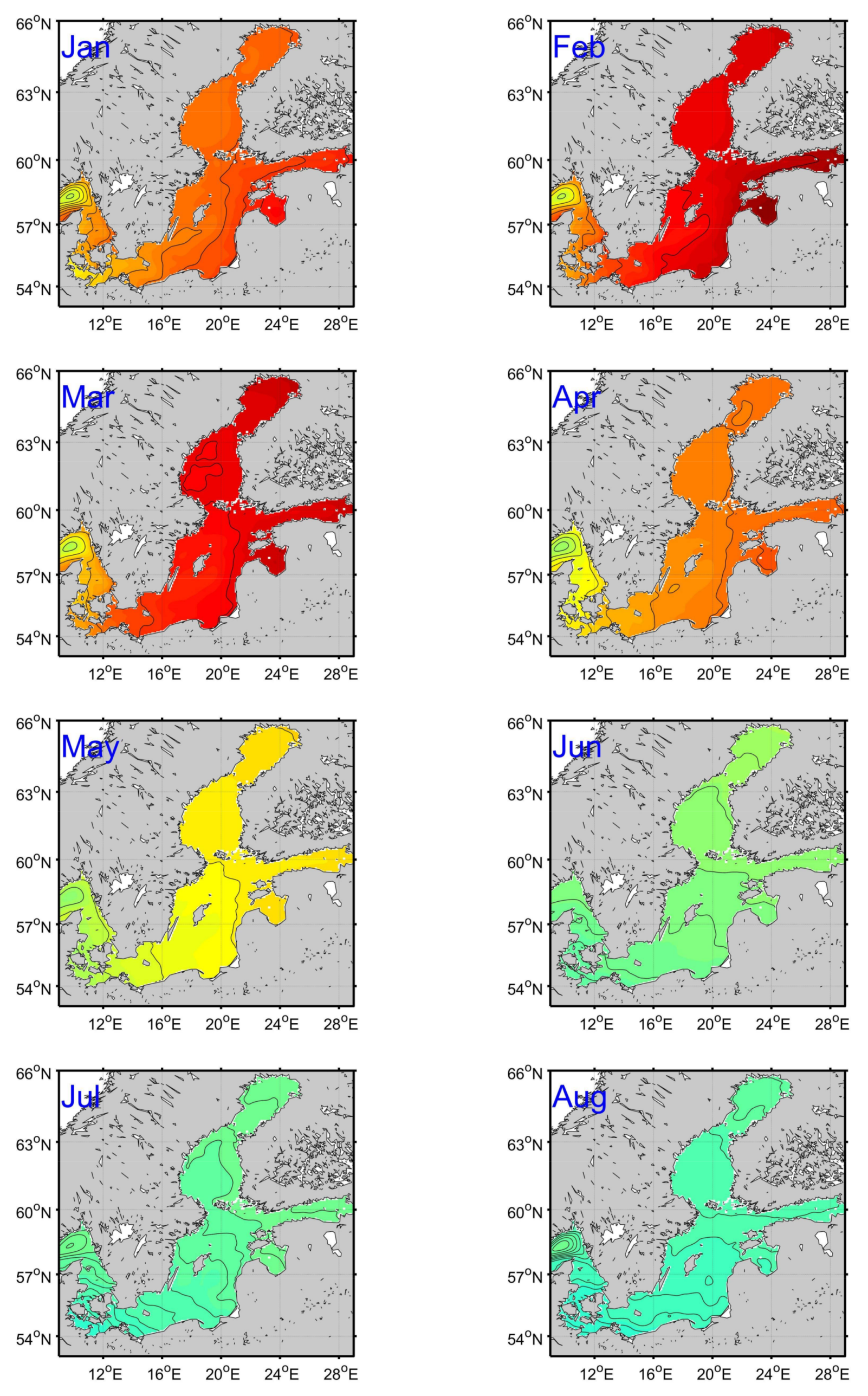

Figure 6.
Geographical distribution of the maximum (a,c) and minimum (multiplied by −1, b,d) annual sea level (cm) estimated from satellite altimetry and tide gauge data (a,b) and SMHI model reanalysis (c,d) the time period 1993–2014.
Figure 6.
Geographical distribution of the maximum (a,c) and minimum (multiplied by −1, b,d) annual sea level (cm) estimated from satellite altimetry and tide gauge data (a,b) and SMHI model reanalysis (c,d) the time period 1993–2014.
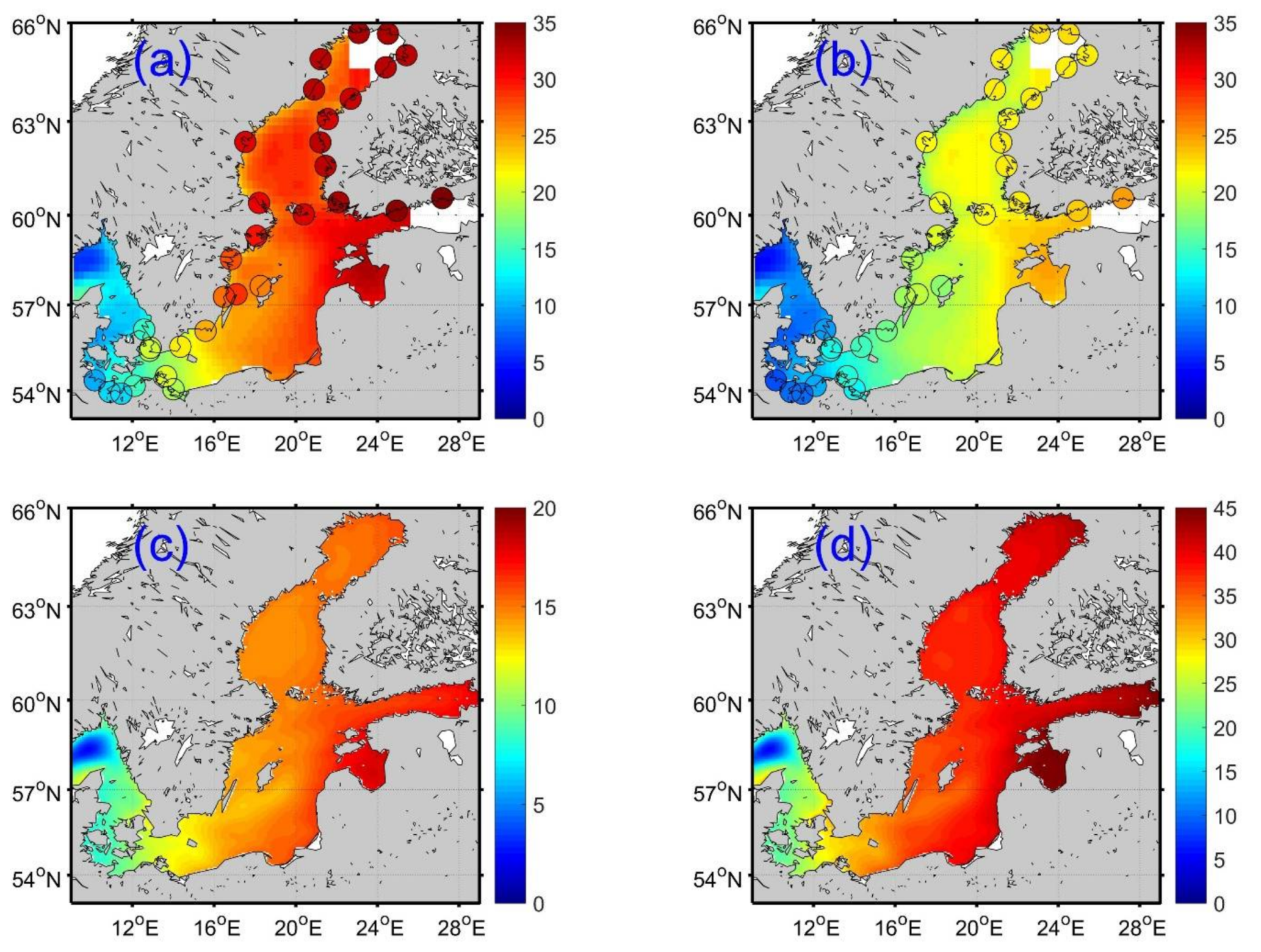
Figure 7.
Similar to Figure 4 but for zonal wind speed (m/s). The CSEOF first mode PC time series (PC1, dimensionless) of sea level (blue line), zonal wind speed (orange solid line), meridional wind speed (orange dashed line) and wind speed (orange dotted line), which denote the interannual variations of the annual cycle in the parameters.
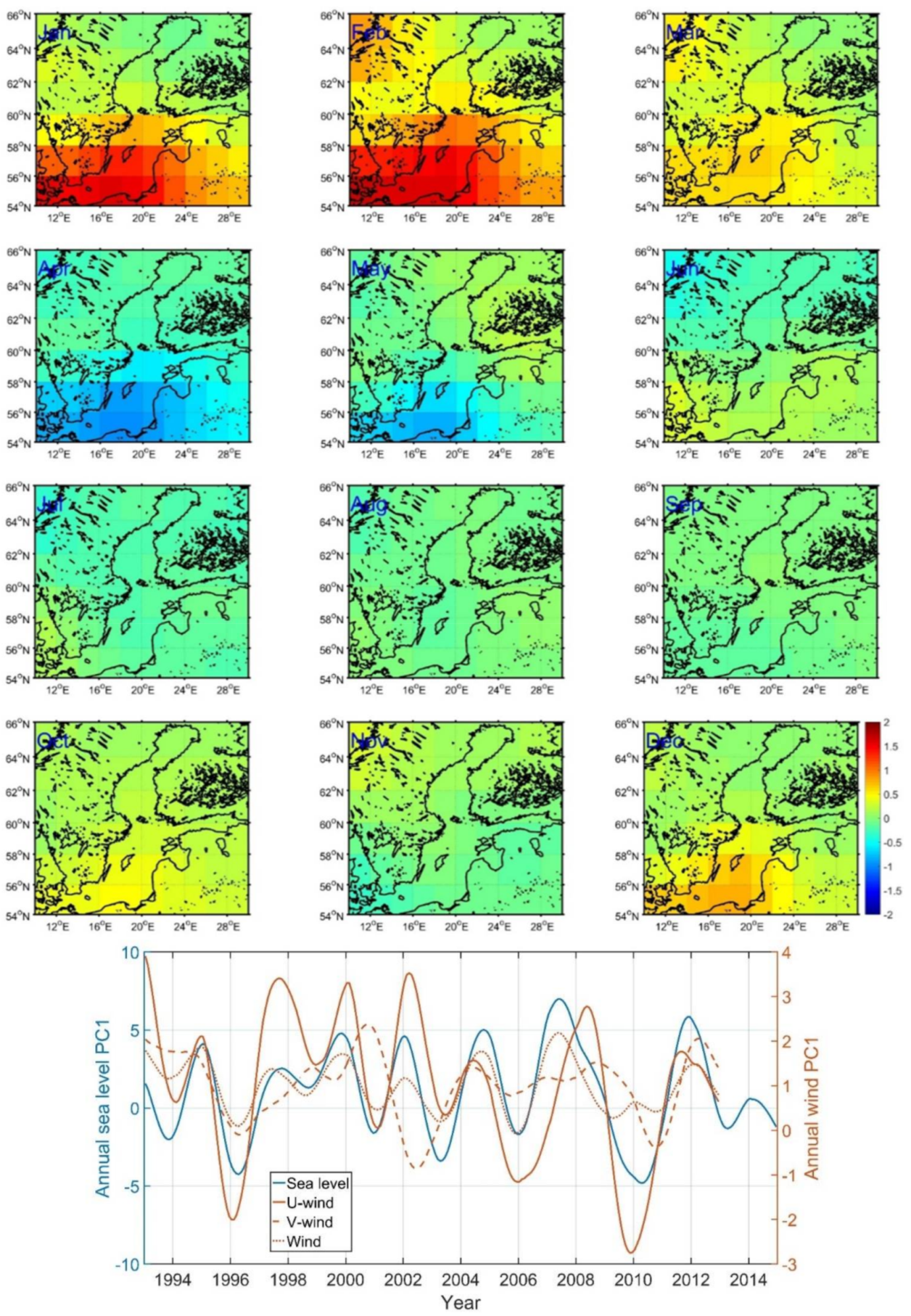
Figure 8.
Average of (a) winter (December–March) and (b) summer (May–August) CSEOF first model LVs (cm) calculated from satellite altimetry and tide gauge data. (c) Average of winter and summer CSEOF first mode PC time series (dimensionless). The station-based winter NAO index (December–March) is overlaid.

Figure 9.
Similar to Figure 4 but for NCEP/NCAR Sea Level Pressure: monthly time-dependent LVs (hpa) and PC time series (computed over the region in Figure 1, dimensionless). The PC time series of annual sea level is overlaid.
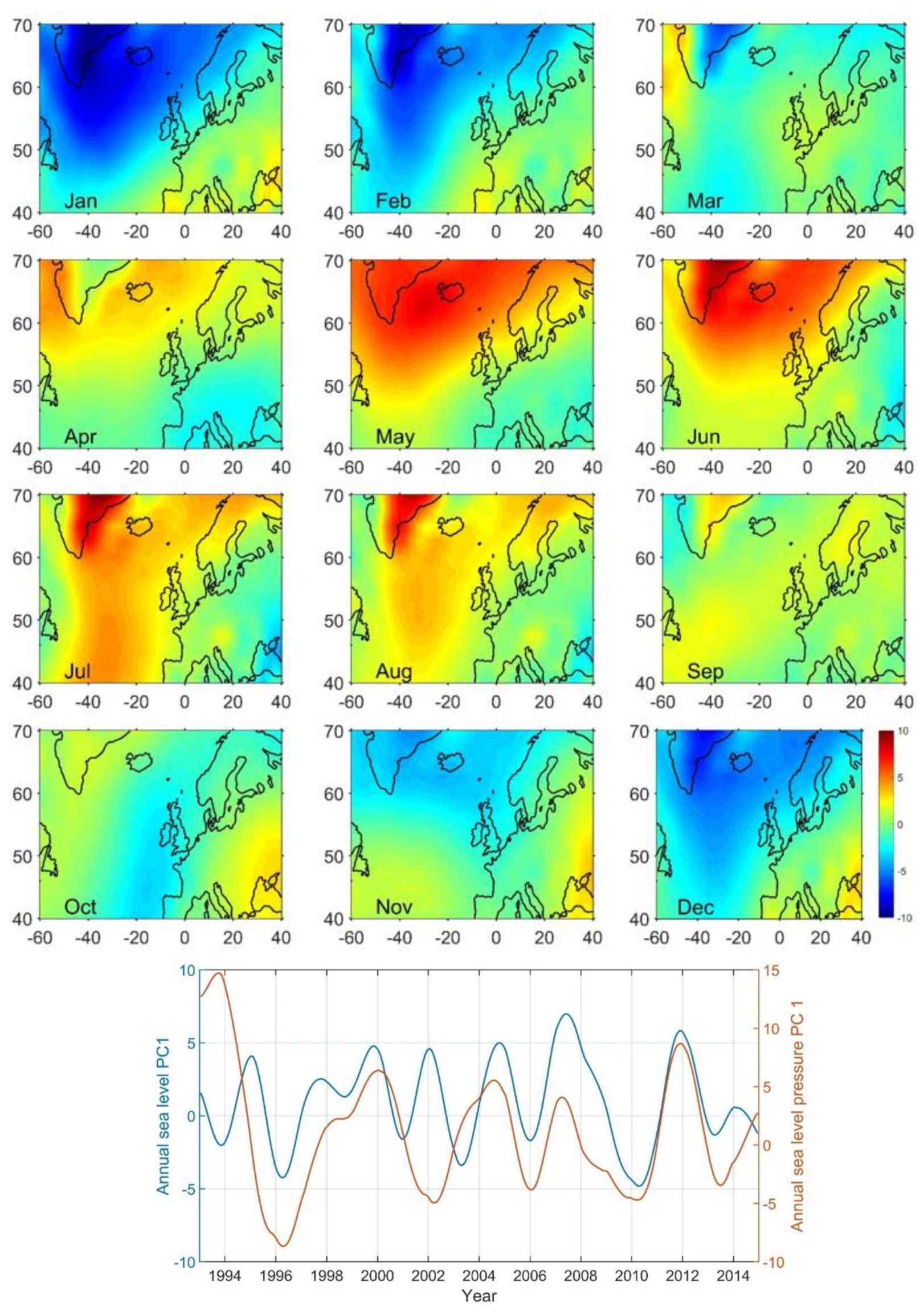
Figure 10.
Similar to Figure 4 but for air temperature: monthly time-dependent LVs (K) and PC time series (computed over the region in Figure 1, dimensionless). The PC time series of the annual sea level is overlaid.

Figure 11.
Spatial pattern of monthly sea ice thickness (m) from the SMHI reanalysis.

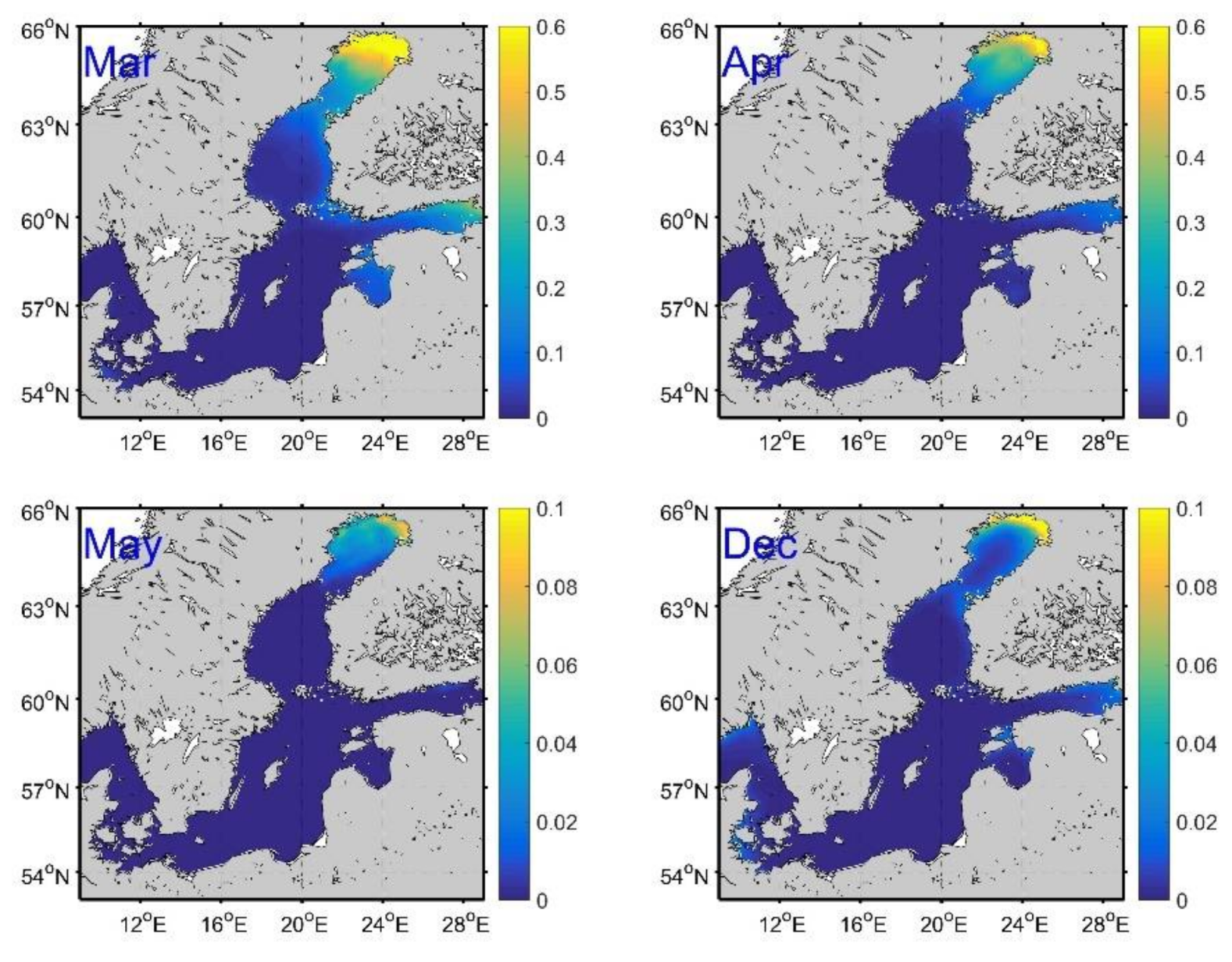
Figure 12.
Annual sea level estimated at (a) Skagsudde (1994–2014) and (b) Klaipeda (1993–2011) using the CSEOF first mode for tide gauge, altimetry data and SMHI analysis.
Figure 12.
Annual sea level estimated at (a) Skagsudde (1994–2014) and (b) Klaipeda (1993–2011) using the CSEOF first mode for tide gauge, altimetry data and SMHI analysis.
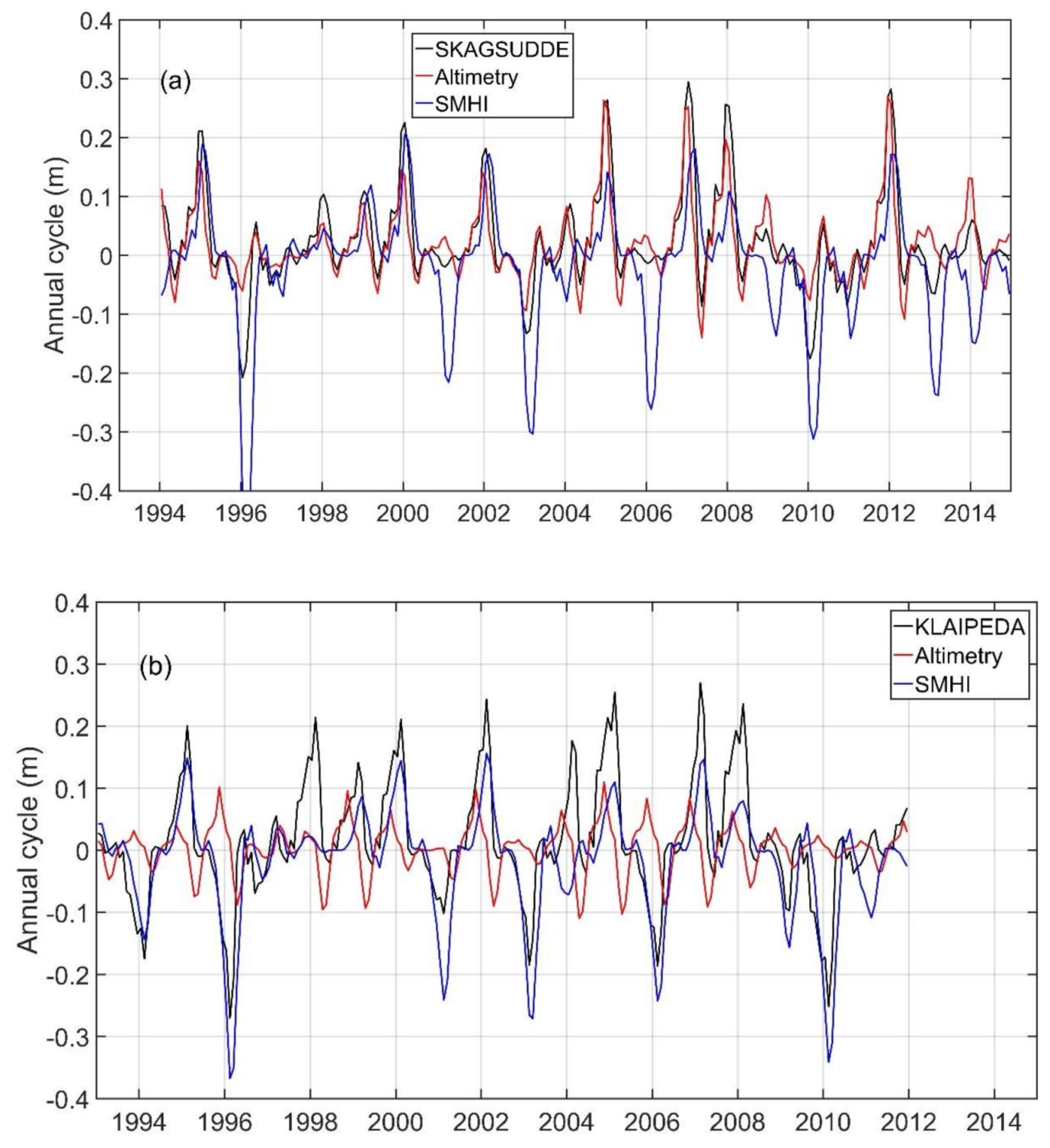
Figure 13.
Annual sea level (m) estimated from tide gauges for the period 1990–2012 using CSEOF first mode.
Figure 13.
Annual sea level (m) estimated from tide gauges for the period 1990–2012 using CSEOF first mode.

Figure 14.
CSEOF first mode PC time series of sea level (cm) at nine tide gauges (Table 2) in 1900–2012. The PC time series of zonal wind (m/s) is overlaid.
Figure 14.
CSEOF first mode PC time series of sea level (cm) at nine tide gauges (Table 2) in 1900–2012. The PC time series of zonal wind (m/s) is overlaid.
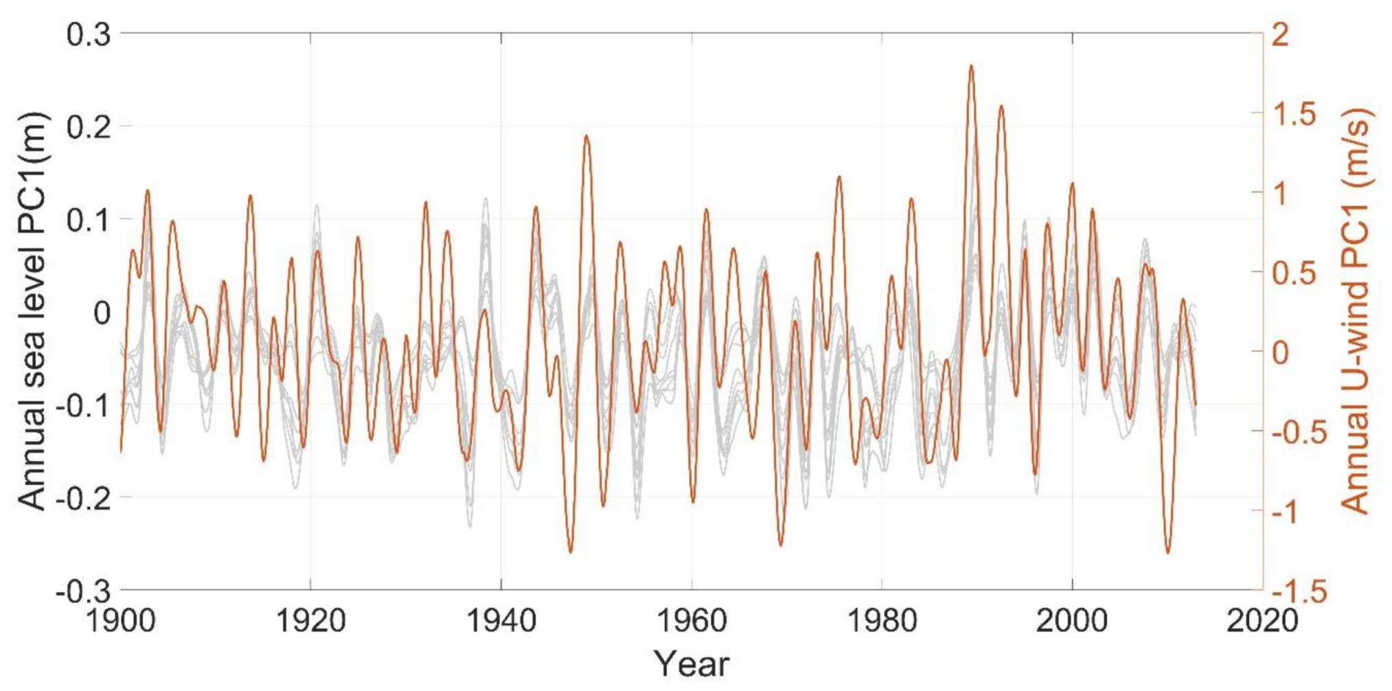
Figure 15.
Average of sea level CSEOF first mode PC time series in winter (December–March) at nine tide gauges (Table 2) in 1900–2012. The PC time series of winter-NAO is overlaid.
Figure 15.
Average of sea level CSEOF first mode PC time series in winter (December–March) at nine tide gauges (Table 2) in 1900–2012. The PC time series of winter-NAO is overlaid.

Table 1.
Tide gauge information used in the present study. (♦ Data valid during 1993–2011. * Data valid during 1993–2012. ** Data valid during 1994–2014. † Data valid during 1900–2012.).
Table 1.
Tide gauge information used in the present study. (♦ Data valid during 1993–2011. * Data valid during 1993–2012. ** Data valid during 1994–2014. † Data valid during 1900–2012.).
| Tide Gauge | Latitude (°N) | Longitude (°E) | Data Availability (%, 1993–2014) | |
|---|---|---|---|---|
| 1 | WISMAR † | 53.900 | 11.458 | 100.00 |
| 2 | WARNEMUNDE † | 54.170 | 12.103 | 100.00 |
| 3 | TRAVEMUNDE | 53.958 | 10.872 | 100.00 |
| 4 | HELSINKI † | 60.154 | 24.956 | 99.62 |
| 5 | VAASA | 63.082 | 21.571 | 89.39 |
| 6 | OLANDS NORRA UDDE † | 57.366 | 17.097 | 100.00 |
| 7 | KUNGSHOLMSFORT † | 56.105 | 15.589 | 100.00 |
| 8 | STOCKHOLM † | 59.324 | 18.082 | 100.00 |
| 9 | OULU | 65.040 | 25.418 | 100.00 |
| 10 | FREDERICIA * | 55.561 | 9.754 | 90.91 |
| 11 | KOBENHAVN * | 55.705 | 12.600 | 86.36 |
| 12 | RATAN † | 63.986 | 20.895 | 100.00 |
| 13 | SLIPSHAVN * | 55.288 | 10.828 | 86.74 |
| 14 | KORSOR * | 55.332 | 11.142 | 90.53 |
| 15 | KLAIPEDA ♦ | 55.700 | 21.133 | 83.71 |
| 16 | HORNBAEK *,† | 56.091 | 12.458 | 89.77 |
| 17 | GEDSER *,† | 54.573 | 11.926 | 90.53 |
| 18 | MANTYLUOTO | 61.594 | 21.463 | 99.62 |
| 19 | PIETARSAARI | 63.709 | 22.690 | 98.86 |
| 20 | FURUOGRUND | 64.916 | 21.231 | 98.11 |
| 21 | KEMI | 65.673 | 24.515 | 100.00 |
| 22 | TURKU | 60.428 | 22.101 | 100.00 |
| 23 | RAAHE | 64.666 | 24.407 | 100.00 |
| 24 | FOGLO | 60.032 | 20.385 | 100.00 |
| 25 | KASKINEN | 62.344 | 21.215 | 100.00 |
| 26 | HAMINA | 60.563 | 27.179 | 99.62 |
| 27 | KLAGSHAMN | 55.522 | 12.894 | 100.00 |
| 28 | SASSNITZ | 54.511 | 13.643 | 100.00 |
| 29 | RODBYHAVN * | 54.656 | 11.349 | 90.91 |
| 30 | KIEL | 54.372 | 10.157 | 100.00 |
| 31 | SPIKARNA | 62.363 | 17.531 | 99.62 |
| 32 | KOSEROW | 54.060 | 14.000 | 98.11 |
| 33 | TEJN * | 55.250 | 14.838 | 89.77 |
| 34 | KALIX | 65.697 | 23.096 | 98.86 |
| 35 | SKAGSUDDE ** | 63.191 | 19.013 | 94.32 |
| 36 | FORSMARK | 60.409 | 18.211 | 100.00 |
| 37 | MARVIKEN | 58.554 | 16.837 | 100.00 |
| 38 | VISBY | 57.639 | 18.284 | 100.00 |
| 39 | OSKARSHAMN | 57.275 | 16.478 | 100.00 |
| 40 | SIMRISHAMN | 55.557 | 14.358 | 100.00 |
| 41 | SKANOR | 55.417 | 12.829 | 100.00 |
| 42 | VIKEN | 56.142 | 12.579 | 100.00 |
Table 2.
Correlations between CSEOF first mode sea level and zonal wind (U-wind), air temperature (Air-t) PC time series, NAO, and winter NAO at WIS (Wismar), WAR (Warnemunde), GED (Gedser), HOR (Hornbaek), KUN (Kungsholmsfort), OLA (Olands Norra Udde), STO(Stockholm), HEL(Helsinki) and RAT (Ratan) over the period 1900–2012.
| WIS | WAR | GED | HOR | KUN | OLA | STO | HEL | RAT | |
|---|---|---|---|---|---|---|---|---|---|
| U-wind | 0.6 ± 0.0 | 0.7 ± 0.0 | 0.6 ± 0.0 | 0.6 ± 0.0 | 0.6 ± 0.0 | 0.5 ± 0.0 | 0.6 ± 0.0 | 0.7 ± 0.0 | 0.5 ± 0.0 |
| NAO | 0.1 ± 0.1 | 0.2 ± 0.1 | 0.1 ± 0.1 | 0.2 ± 0.1 | 0.3 ± 0.1 | 0.2 ± 0.1 | 0.3 ± 0.1 | 0.3 ± 0.1 | 0.2 ± 0.1 |
| Winter-NAO | 0.4 ± 0.2 | 0.4 ± 0.2 | 0.4 ± 0.2 | 0.5 ± 0.1 | 0.6 ± 0.1 | 0.5 ± 0.1 | 0.6 ± 0.1 | 0.6 ± 0.1 | 0.5 ± 0.1 |
| Air-t | −0.2 ± 0.1 | −0.2 ± 0.1 | −0.1 ± 0.1 | −0.0 ± 0.1 | −0.0 ± 0.1 | 0.0 ± 0.1 | 0.0 ± 0.1 | −0.0 ± 0.1 | 0.0 ± 0.1 |
© 2018 by the authors. Licensee MDPI, Basel, Switzerland. This article is an open access article distributed under the terms and conditions of the Creative Commons Attribution (CC BY) license (http://creativecommons.org/licenses/by/4.0/).
Share and Cite
MDPI and ACS Style
Cheng, Y.; Xu, Q.; Li, X. Spatio-Temporal Variability of Annual Sea Level Cycle in the Baltic Sea. Remote Sens. 2018, 10, 528. https://doi.org/10.3390/rs10040528
AMA Style
Cheng Y, Xu Q, Li X. Spatio-Temporal Variability of Annual Sea Level Cycle in the Baltic Sea. Remote Sensing. 2018; 10(4):528. https://doi.org/10.3390/rs10040528
Chicago/Turabian StyleCheng, Yongcun, Qing Xu, and Xiaofeng Li. 2018. "Spatio-Temporal Variability of Annual Sea Level Cycle in the Baltic Sea" Remote Sensing 10, no. 4: 528. https://doi.org/10.3390/rs10040528
Note that from the first issue of 2016, this journal uses article numbers instead of page numbers. See further details here.