Integrating Airborne LiDAR and Optical Data to Estimate Forest Aboveground Biomass in Arid and Semi-Arid Regions of China


1
College of Resources and Environmental Sciences, Nanjing Agricultural University, Nanjing 210095, Jiangsu, China
2
Department of Geography & Spatial Information Techniques, Ningbo University, Ningbo 315211, Jiangsu, China
*
Author to whom correspondence should be addressed.
Remote Sens. 2018, 10(4), 532; https://doi.org/10.3390/rs10040532
Submission received: 4 December 2017
/
Revised: 25 February 2018
/
Accepted: 28 March 2018
/
Published: 30 March 2018
(This article belongs to the Special Issue Biomass Remote Sensing in Forest Landscapes)
Abstract
:Forest Aboveground Biomass (AGB) is a key parameter for assessing forest productivity and global carbon content. In previous studies, AGB has been estimated using various prediction methods and types of remote sensing data. Increasingly, there is a trend towards integrating various data sources such as Light Detection and Ranging (LiDAR) and optical data. In this study, we constructed and compared the accuracies of five models for estimating AGB of forests in the upper Heihe River Basin in Northwest China. The five models were constructed using field and remotely-sensed data (optical and LiDAR) and algorithms including Random Forest (RF), Support Vector Machines (SVM), Back Propagation Neural Networks (BPNN), K-Nearest Neighbor (KNN) and the Generalized Linear Mixed Model (GLMM). Models based on the RF algorithm emerged as being the best among the five algorithms irrespective of the datasets used. The Random Forest AGB model, using only LiDAR data (R2 = 0.899, RMSE = 14.0 t/ha) as the input data, was more effective than the one using optical data (R2 = 0.835, RMSE = 22.724 t/ha). Compared to LiDAR or optical data alone, the AGB model (R2 = 0.913, RMSE = 13.352 t/ha) that used the RF algorithm and integrated LiDAR and optical data was found to be optimal. Incorporation of terrain variables with optical data resulted in only slight improvements in accuracy. The models developed in this study could be useful for using integrated airborne LiDAR and passive optical data to accurately estimate forest biomass.

1. Introduction
Forests are the dominant carbon stock in terrestrial ecosystems and play a vital role in reducing concentrations of greenhouse gases in the atmosphere and slowing down global warming [1,2]. Forest Aboveground Biomass (AGB) is a key biophysical parameter for measuring carbon and is generally used to quantify the contribution of forests to the global carbon cycle [3]. Therefore, rapid and accurate estimation of forest aboveground biomass can greatly reduce the uncertainty in carbon stock assessments [4]. Traditional methods used to estimate forest AGB based on field measurements or long-term forest inventories can accurately obtain forest AGB, but are usually time-consuming and labor-intensive [5,6,7]. Remote-sensing technologies provide quick and repeated information about wide geographical areas that can be effectively used for estimating forest AGB [8,9].
Various types of remote-sensing data are used for forest biomass estimation: optical sensor data, radio detection and ranging (radar) data, Light Detection And Ranging (LiDAR) data [10], etc. Each of these data sources has its own advantages and disadvantages for estimating forest biomass. Optical sensors were first applied to the remote sensing of forests because they give aggregate spectral signatures (reflectance or vegetation indices) and can be used to retrieve horizontal forest structure, such as type and canopy cover [11,12,13,14]. The characteristics of optical data with long observation times, wide spatial coverage and multiple bands can provide abundant information about forest structure [15,16]. There are many studies utilizing moderate spatial resolution sensor data (e.g., MODIS and TM) for forest biomass estimation [12,17]. However, moderate spatial resolution data lose more spatial detail of AGB variability relative to high-resolution satellite data (e.g., ZY-3 and SPOT). SPOT can provide high spatial information with respect to the size of vegetation units [18]. Especially, ZY-3, which was designed for the collection of stereo imagery, has a better performance on the description of forest structures [16,19,20]. Although optical data are widely used in AGB estimation, widespread use is limited by frequent cloud cover in mountainous regions and data saturation problems in areas with high vegetation biomass or canopy density [15]. Unlike passive optical systems, radar data will penetrate through clouds and forest canopies, but signal saturation poses a problem [21,22]. A good alternative to optical and radar data is LiDAR data, an active remote-sensing technology that can capture the vertical structure of a forest in great detail and provide 3D information, which is strongly related to forest biomass [23]. LiDAR data have been widely used for estimating forest biomass in both natural and human-modified landscapes [24,25,26]. Spaceborne LiDAR, such as the Geoscience Laser Altimeter System (GLAS), can capture large-area forest biomass and update information regularly. Compared to spaceborne LiDAR, airborne LiDAR data are collected over small to moderate spatial extents and at a high resolution, thus making it possible to estimate forest biomass more accurately [27].
Optical data can provide complementary texture and spectral information to the forest 3D structure, which is derived from LiDAR data, and the accuracy of forest biomass estimates could be improved by a combined use of LiDAR and optical data [12]. Su et al. [28] used a combination of spaceborne LiDAR, optical imagery and forest inventory data to estimate the spatial distribution of forest aboveground biomass in China and found that improved estimation accuracy of forest AGB can be achieved. Hong et al. [29] estimated forest AGB using GLAS LiDAR and Landsat TM data for Changbai Mountain in China, and it was found that the accuracies of the forest AGB model that used integrated data were significantly improved compared to those that used GLAS LiDAR alone. In addition, some research explored the potential of integrated LiDAR and optical data for the estimating forest biomass. Luo et al. [30] showed that the fusion of airborne LiDAR data and optical imagery for forest biomass estimation can improve R2 by 2.2% and reduce RMSE by 1.1%, when compared with LiDAR data alone. Brovkina [31] and Swatantran et al. [32] used the integration of LiDAR and hyperspectral data to estimate biomass, and they found that fused data generated a better predicted result than other data.
Different methods have been used to estimate forest biomass and can be divided into two categories: parametric and nonparametric algorithms [33]. The parametric algorithms usually refer to the common statistical methods (e.g., linear regression models). However, there is no simple linear relationship between remote sensing data and forest biomass, as the latter is affected by many factors. Non-parametric techniques including machine learning techniques such as Back Propagation Neural Network (BPNN), K-Nearest Neighbor (KNN), Support Vector Machine (SVM) and Random Forest (RF) have a higher ability to identify complex relationships between predictor and dependent variables and have subsequently have yielded better results [34,35]. The distribution of forest types was influenced by the slope aspect of terrain, especially for the mountain regions [36,37,38]. However, there are still too few research works that have explored the effects of topography in the process of estimating forest biomass. Consequently, we analyzed the effect of additional terrain data on the model accuracy of forest biomass.
Although various remote sensing data and modeling methods have been adopted in forest biomass estimation, there is no universal model for accurate estimation [39]. Therefore, it is important to compare the prediction accuracy of the model using different remote sensing data and modeling methods. Remote sensing data, which matched the resolution of the field plot area, were chosen as the input data, and five prediction methods (RF, SVM, BPNN, KNN and Generalized Linear Mixed Model (GLMM)) were used to quantify the relationship between the remote-sensing variables and measured AGB in the field plots. In this study, our aim was to explore the best methods and optimal kinds of remote sensing data for forest AGB estimation. Finally, we discuss the effects of terrain variables on estimating forest AGB.
2. Materials and Methods
2.1. Study Area
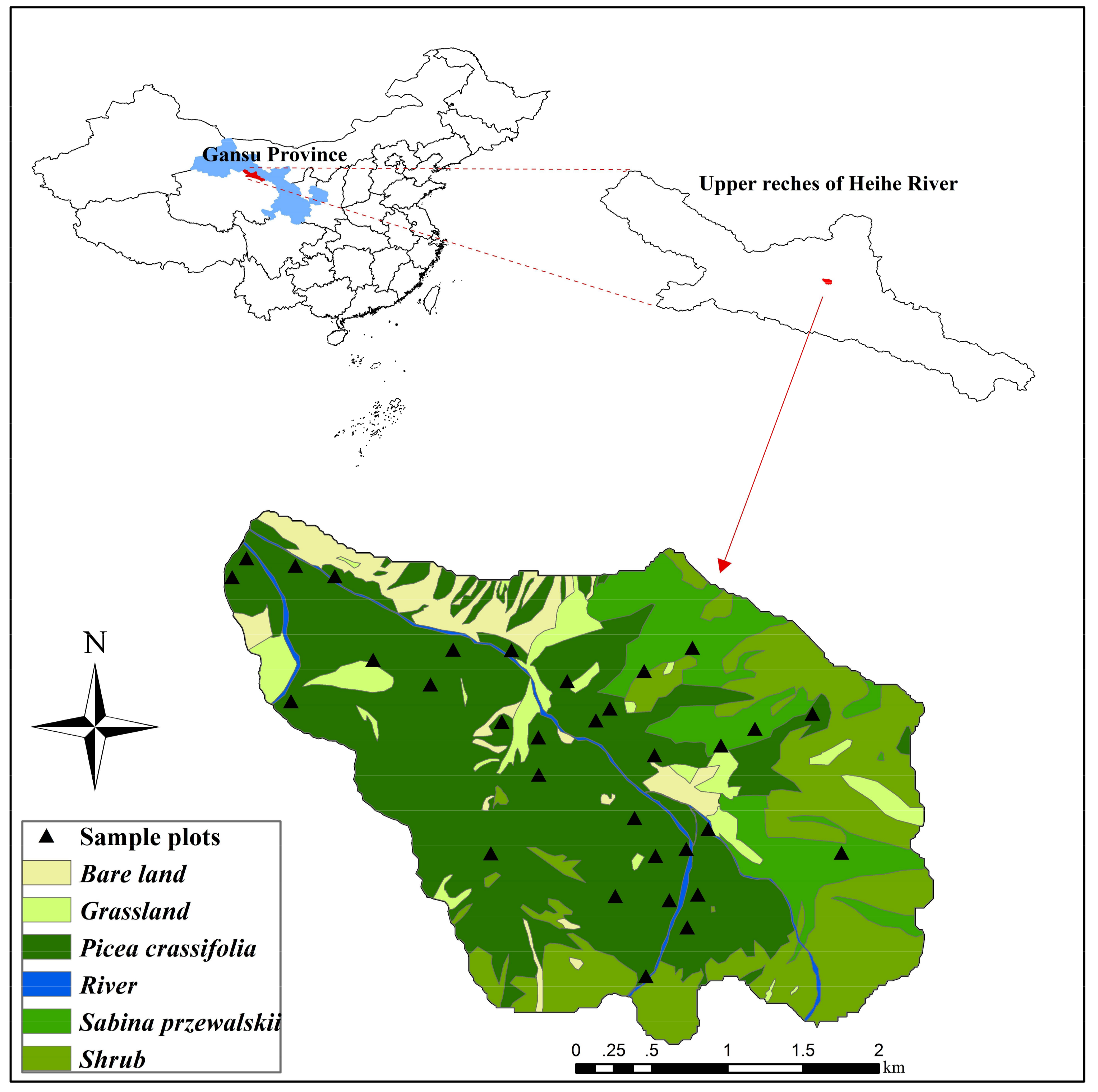
The study area is located in the Tianlaochi Catchment (38°24′ to 38°26′N, 99°53′ to 99°56′E), measuring 10.247 km2, and is one basin of the upper reaches of the Heihe River in the province of Gansu in Northwest China (Figure 1); it belongs to the arid and semi-arid region. The area is in a mountainous region located on the northern slope of Qilian Mountain; the elevation gradually reduces from northeast to southwest. The topography is rough, with steep slopes and deep valleys, and the elevation ranges from 2500 m–3200 m. The mean annual temperature is from −0.6–2.4 °C, and mean annual rainfall is from 400 mm–600 mm, falling mainly from May–September. The site consists of native coniferous forest with moderately dense canopy cover, spreading along a topographically-mountainous terrain. The dominant vegetation types are forest, which include spruce (Picea crassifolia) and cypress (Sabina przewalskii); we mainly assess the forest biomass of these species in our study. Other vegetation types, such as shrubs (Dasiphora fruticosa, Caragana jubata, etc.) and meadow, occasionally occur in the area. The study area is located in a natural forest area, and most parts of the area consist of naturally-regrowing secondary forest. The vegetation density is generally high, due to the lack of management activities.
2.2. Field Measurement
Field data measurements were carried out on 18 July and 12 August 2012. Due to the forest landscape types being simple, we selected 32 typical sample plots with a size of 20 m × 20 m by referring to previous studies [30,33]. The center coordinates of the sample plots used the Real-Time Kinematic (RTK) Global Positioning System (GPS). RTK-GPS is one of the most precise positioning technologies with which users can obtain cm-level accuracy of a position in real time [40]. Twenty seven sample plots were distributed in the Picea crassifolia forest, and five sample plots were distributed in the Sabina przewalskii forest. For each sample plot, we measured tree height (H, m) and Diameter at Breast Height (DBH, only trees with DBH ≥5 cm were counted). Single tree biomass values were obtained using allometric equations for water conservation forest developed by Wang et al. [41] in Northwest China. Following the estimation of single tree biomass values, we then calculated the biomass using the total biomass in each plot (sum of single tree biomass in the field plot) by conversion to tons per hectare unit. The forest aboveground biomass values varied from 16.37 t/ha–207.67 t/ha, with a mean value of 101.973 t/ha and standard deviation of 46.893 t/ha.
2.3. Optical Data
Optical data that contained spatial information have been widely used for forest AGB estimation. We utilized data to estimate forest biomass from the Chinese satellite ZiYuan-3 (ZY-3) with a resolution of 3.6 m for forward and backward views and 2.1 m for the nadir view. The ZY-3 data were acquired during the time of the field measurement dates, which must cover the study region. The test image was collected on 26 July 2012, and then, the Digital Number (DN) needed to be converted to reflectance values in the preprocessing stage, which was performed using ENVI 5.3 software. Radiometric calibration, atmospheric correction and topography correction were applied to the ZY-3 data. In order to estimate the optical properties of terrestrial surfaces, it was necessary to eliminate the radiative components due to the atmosphere. The data were converted to top-of-atmosphere reflectance, the calibration coefficients of which were provided by China Centre for Resources Satellite Data and Application; atmosphere correction was performed using the Fast Line-of-sight Atmosphere Analysis of Spectral Hypercube (FLAASH). Finally, because there are many mountains in the study area, we had to perform topography correction using the sun-canopy-sensor with C-correction (SCS + C) method using Digital Elevation Model (DEM) data, which was performed using ENVI 5.3 software.
2.4. Airborne LiDAR Data
Airborne LiDAR data were collected on 25 August 2012, using a Leica Airborne Laser Scanner (ALS70) [42]. The ALS70 airborne laser scanning system is mainly composed of a system controller, laser controller, camera controller, laser scanner and operating and navigation terminal. The top pulse frequency, maximum sweep frequency and maximum scan angle were 500 kHz, 200 Hz and 18°, respectively. The average point density of LiDAR data covering the study region was 1 point/m2, with a laser beam diameter that reached the ground at 0.35 m. A dual-frequency Differential Global Positioning System (DGPS) and Inertial Measurement Unit (IMU) were adopted in the LiDAR system, which can achieve precise positioning. The horizontal and vertical accuracy of the ground points of the LiDAR data were 0.1 m and 0.3 m. LiDAR data were originally acquired in GCS (Geographic Coordinate System), but were later projected to UTM Zone 47 N. For this study, all laser returns are included in the analyses. Thus, the Gaussian filter was used for the LiDAR point cloud, and this was classified into ground and non-ground points using LiDAR data processing software (TerraScan, TerraSolid, Ltd., Helsinki, Finland). Then, the point cloud was interpolated into a Digital Terrain Model (DTM) and a Digital Surface Model (DSM) with a 2-m spatial resolution. A Canopy Height Model (CHM) was produced by subtracting DTM and DSM. These normalized point cloud data were further processed to derive metrics representing the height of the trees in the plot. The relative canopy structure information was extracted by the intensity of point cloud data.
2.5. Optical Features Extraction for Forest Biomass Estimation
2.5.1. Vegetation Indices
Vegetation Indices (VIs) can reflect the growth tendency of tree and have a better correlation with vegetation biomass; they were generally used as variable predictors in the biomass model [43]. In particular, VIs can reduce the influence of soil background, atmosphere and water for the vegetation reflectance [44,45]. Various VIs derived from optical data were used to estimate biomass, but there was no universal index applied to all vegetation. Four kinds of vegetation indices (Table 1), Ratio Vegetation Index (RVI), Normalized Difference Index (NDVI), Soil-Adjusted Vegetation Index (SAVI) and Modified Soil-Adjusted Vegetation Index (MSAVI), were calculated from the bands of ZY-3 data.
2.5.2. Texture Information
When we manipulate multivariate data, some information is potentially redundant. Therefore, utilizing a simplified index to reserve original information will reduce the calculations and volume of data. Among the many existing methods for reducing dimensionality, the most popular is Principal Component Analysis (PCA) [46], which can be performed to reduce the redundancy of information. We conducted PCA for the all bands of the ZY-3 data; the results can be used as the input factor for the model of forest AGB estimation.
The potential of textural information from satellite images has been clearly demonstrated in the estimation of forest biomass [47]. Texture information is the main characteristic of remote sensing data; it can reveal the relationship between structure features of ground objects and the surrounding environment and reflect the spatial variations of cover type at the same time. Texture information is usually extracted from images using statistical, structural and spectral methods [48]. We adopted a texture analysis method based on the Gray-Level Co-occurrence Matrix (GLCM) in our study. Eight texture variables were selected, the Mean (ME), Variance (VA), Homogeneity (HO), Contrast (CO), Dissimilarity (DI), Entropy (EN), Second Moment (SM) and Correlation (CR), and their values were determined according to Equations (1)–(8). Texture analysis was carried out based on the first component, which was the result of PCA; the size of the window is 3 × 3.
2.6. LiDAR Features Extraction for Forest Biomass Estimation
2.6.1. LiDAR-Derived Variables
The LiDAR point cloud is characterized by a certain number of features, mostly calculated by analyzing the distribution of its neighboring points, which have the same characteristics [49]. Forest AGB was closely related to tree height, and we selected metrics, such as the max (Hmax), mean (Hmean), standard deviation (HSD) and coefficient of variation (HCV) of the tree height in the sample plot. The metrics derived from LiDAR point cloud data were identified in previous studies as predictor variables to estimate forest AGB [38,50,51].
In LiDAR data, the intensity of the point clouds was generally used to distinguish among the ground points and tree species, and many studies used point clouds along with laser intensity to obtain canopy structure information [52]. Canopy cover, which was defined as the fraction of ground covered by vegetation canopy, had a strong correlation with forest AGB [53,54,55]. Canopy cover (Cc) was calculated as the ratio of canopy intensity sums and all intensities Cc (see Equation (9)) within each subplot [51,56]. The represented LiDAR metrics, such as canopy cover, vegetation intensity, the max, mean, standard deviation and coefficient of variation heights (Table 2), were obtained from the height-normalized point clouds by analysis in the LiDAR 360 Tools. In the operation process, layers with a 20-m resolution were generated using the 2-m vegetation height threshold.
where Icanopy is the canopy intensity sums and the Iground is ground intensity sums.
2.6.2. Terrain Variables
Data from airborne LiDAR can provide high-resolution terrain information of the Earth’s surface [57]. We use terrain variables extracted from LiDAR ground points with a resolution of 20 m (Table 2). The Topographic Wetness Index (TWI) is similar to the Wetness Index (WI) and was developed by O’Loughlin [58]; TWI quantifies the level of soil water storage and drainage. Profile Curvature (PC) describes the variation of slope and influences the speed of movement, deposition and erosion on the Earth’s surface. Hillshade, which represents topographic shadowing, is calculated using an azimuth angle of 180° and a zenith of 30°, according to the specified altitude of the Sun. Slope has a close relation with the stability of soil, and it can reflect the tilt level of the local topography. Calculation of slope, hillshade, TWI and PC was implemented in SAGA GIS (System for Automated Geoscientific Analyses Version 2.1.4, available at http://www.saga-gis.org). These four variables are important for quantifying the effects of topography on hydrological processes where hydrological data are lacking.
2.7. Statistical Analysis and Modeling
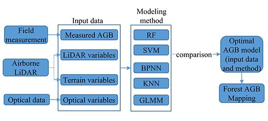
Five combinations of data variables were used to estimate forest AGB: LiDAR variables (LVs), optical variables (OVs), LiDAR and optical variables (LVs + OVs), LiDAR and terrain variables (LVs + TVs) and optical and terrain variables (OVs + TVs). The predictor variables (9 variables for LiDAR data and 12 variables for ZY-3 data) and corresponding AGB field data were used to estimate forest AGB. Five parametric or nonparametric methods were considered: the five abovementioned modeling methods (RF, SVM, BPNN, KNN and GLMM) and five input datasets were applied to build forest AGB prediction models, respectively; 25 models were obtained in the results.
RF is a classification and regression tree approach that is often efficient in the predictive model [59], with each tree randomly selected from the subsets of predictor variables. The number of trees (ntree) is yielded by the original data, based on a bootstrap sample, which was determined from the relationship between N and the error. For each regression tree, the number of different predictors tested at each node (mtry) was selected based on the RMSE of the data. SVM is a training approach that is widely used in classification and regression analysis; it has an efficient capacity of generalization [60]. BPNN is one of the most popular algorithms in the neural network, which has potential for estimating forest biomass, as it can deal with complex linear or nonlinear relationships of reflectivity data and vegetation parameters [61]. Typically, the KNN method is frequently applied to a model when the number of samples is small, and given that the redundancy of the result is low, it is suitable for forest biomass estimation at a regional scale [62]. GLMM is a regression model that includes random effects in order to have a wide range of dependent variables through linear combinations of one or multiple predictor variables [63]. The packages and parameters of the five methods used in the R statistical software are shown in Table 3.
To assess the reliability and accuracy of forest AGB estimation models, the most common measures in the reviewed research were R2 (correlation between observed and predicted values) and Root Mean Square Error (RMSE). The RMSE was calculated using Equation (10), which can predict AGB versus the AGB measured from field observations. As there were no additional data available for estimating the accuracy of the prediction models. The Leave-One-Out Cross-Validation (LOOCV) method, an effective method to evaluate the generalization capability of regression models, was used [64]. All statistical calculations were performed in the R statistical package.
where represents the predicted biomass of sample i, represents the filed-measured biomass and n represents the total number of samples.
3. Results
3.1. Comparison of Forest AGB Estimation Using Various Data Types
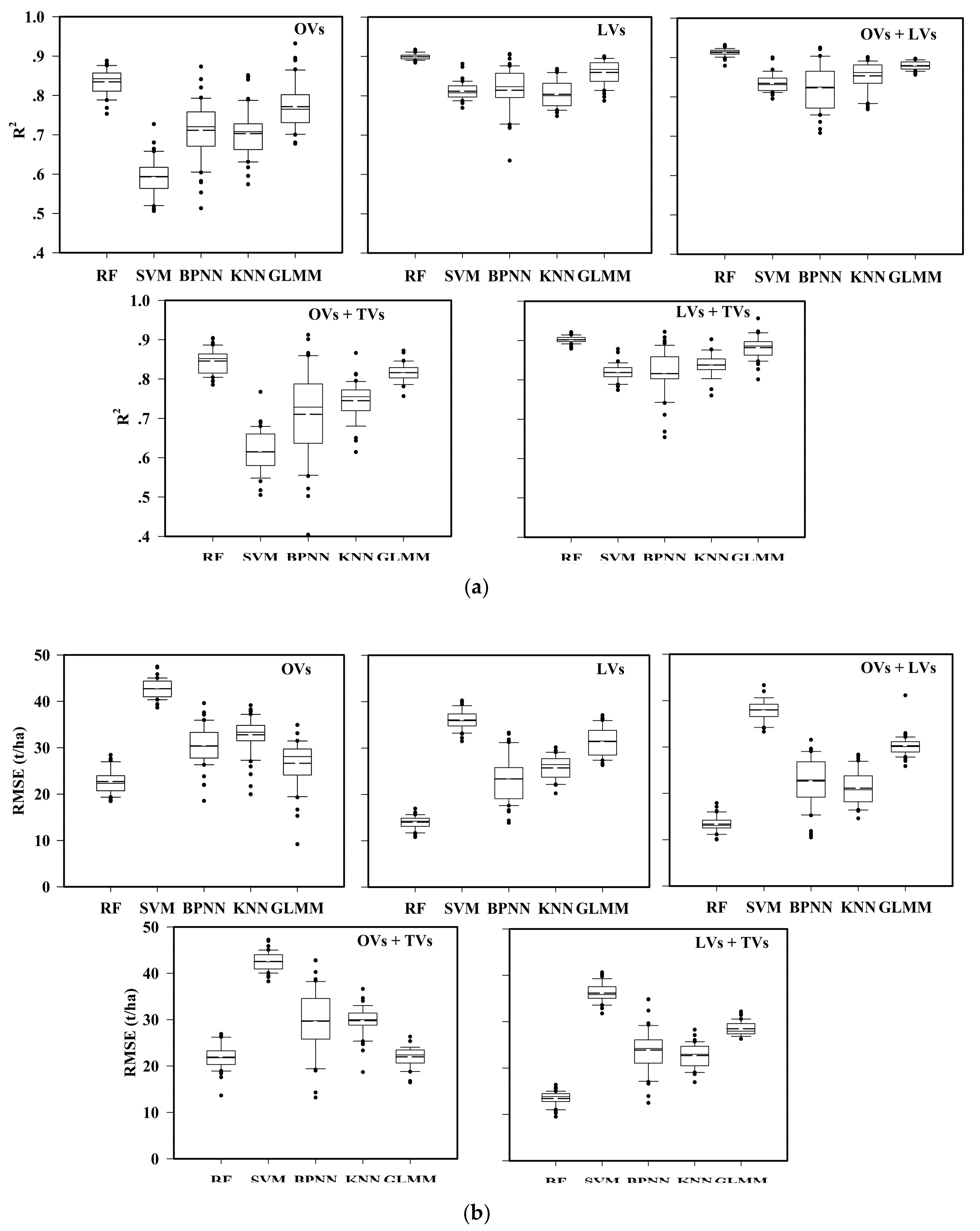
The performances of models using all data types, evaluated according to R2 and RMSE, are shown as boxplots in Figure 2a,b. A comparison across the five data types indicated that integrated LiDAR and optical data outperformed all other tested datasets; LVs + TVs performed almost as well. Comparing the accuracy of the model using a single data source for estimating forest AGB, LiDAR data as input variables were more effective than optical data. For LiDAR and optical data alone, the highest R2 values for forest AGB estimation were 0.899 (RMSE = 14.0 t/ha) and 0.835 (RMSE = 22.724 t/ha), respectively. The biggest variation of estimation accuracies between LiDAR and optical data was in models using the SVM method, and the values reached 0.21 for R2 and 7.06 t/ha for RMSE. The results showed that LiDAR data had a better relationship with the observed forest AGB than optical data.
Models incorporating terrain data produced better accuracies than those built solely based on LiDAR or optical data. The accuracies of mean R2 were slightly increased, and RMSE obviously decreased using the five methods (Figure 2). The highest estimation accuracies of LiDAR and optical data, when adding terrain variables separately, were 0.902 (RMSE = 13.45 t/ha) and 0.846 (RMSE = 21.923 t/ha). Model accuracy was slightly improved by incorporating additional terrain variables, especially for optical data. For all prediction methods, only marginal differences in RMSE and R2 were observed when comparing models using LiDAR or the integrated LiDAR and terrain data. Compared with the optical data as input variables alone, the accuracies of mean R2 when adding terrain data are increased in the five methods, and the RMSE decreased, especially for the KNN and GLMM methods with RMSEs of 29.784 t/ha and 21.973 t/ha, respectively. These indicated that optical data are affected by terrain more than LiDAR data in terms of forest biomass estimation.
According to Figure 2, the differences between model accuracy of LiDAR-only and combined LiDAR and optical data were distinct. Compared with the LiDAR metrics alone, the AGB model using integrated data had an improved estimation accuracy with an RMSE that decreased from 0.6 t/ha to 4.6 t/ha and an R2 that increased from 0.009 to 0.05. The accuracies of R2 were obviously improved in three models: SVM (R2 = 0.834), KNN (R2 = 0.853) and GLMM (R2 = 0.879), and the mean RMSEs were significantly reduced in the KNN models; the decreased proportion was nearly 17%. Integrated LiDAR and optical data produced the best estimation accuracies with the highest R2 and a lower RMSE among the five datasets of the input variables (OVs, LVs, OVs + TVs, LVs + TVs), especially when the RF method was used (R2 = 0.913, RMSE = 13.352 t/ha). LiDAR data have an unparalleled advantage over other remote-sensing data, but at a high cost. Optical data are less expensive; however, they are vulnerable to the effects of saturation. Therefore, it is essential for extracting useful information from a large amount of data and utilizing the advantages of multivariate remote sensing data, thereby improving the accuracy of forest biomass estimation.
3.2. Optimal Prediction Methods for Forest AGB Estimation
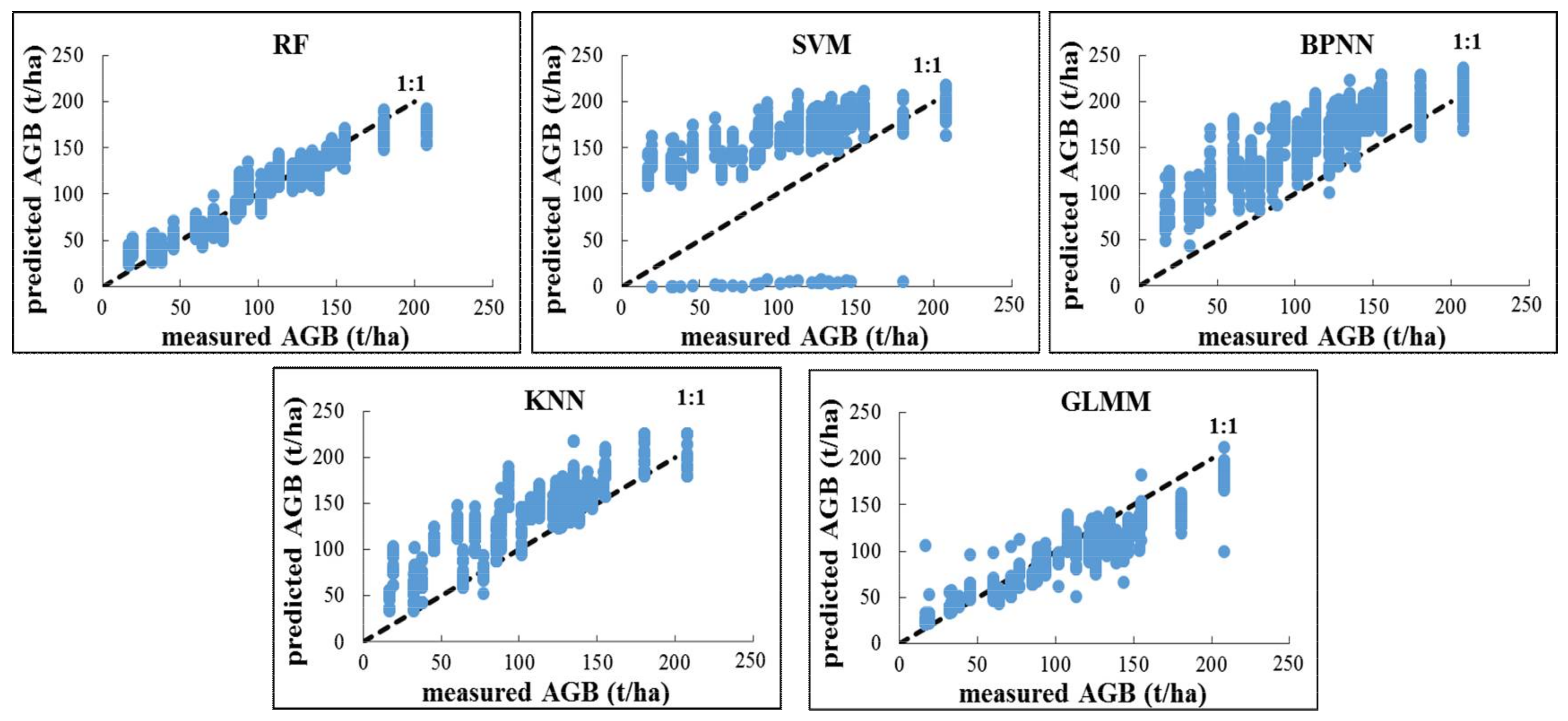
A comparison of the results obtained using the different methods is presented (Figure 3); the model with the RF method showed the best predicted accuracy, based on all of the data types. The performance of the SVM AGB models for modeling accuracy was the worst in terms of R2 and RMSE among all methods tested. We assumed that this was due to the fact that they give poor results if the number of features is much greater than the number of samples. Although the GLMM AGB model had a relatively high R2, it also had a high RMSE, implying that the model was unstable. The observed results concerning the prediction methods always exhibited a worse performance by BPNN and KNN for forest AGB estimation, which may be strongly dependent on the relationship of the training dataset with the prediction results. Outliers and erroneous values in the training data may reduce the model accuracy. The complex relationship between forest AGB and remote sensing variables cannot be well-explained using a simple linear model. The RF model, based on the machine learning method for classification and regression, enabled the diversity of the relationships between the predictor variables and the forest biomass to be taken into account in the studied area.
The performance of the model that used the RF, SVM, BPNN, KNN and GLMM methods was further analyzed. Scatter plots of measured forest AGB against predicted data based on optical and LiDAR data used five methods with 50 bootstraps (shown in Figure 4). The distribution of scatter points is concentrated near the 1:1 line; the figure shows that SVM, BPNN, KNN and GLMM overestimated forest AGB, especially SVM, which had a number of outliers in the results. The GLMM AGB model has predicted AGB values distributed near the 1:1 line, but it had some dispersive outliers. This phenomenon indicated that the GLMM method was unstable. The RF method was more stable than the other methods, although the model overestimated forest AGB at low levels (0–120 t/ha) and underestimated data at high value levels (120–250 t/ha), especially at levels with values greater than 180 t/ha. Thus, the results of the models, using different datasets and the five modeling methods, showed that RF was the best method among all models, regardless of the types of datasets used.
3.3. Mapping the Forest AGB Distribution
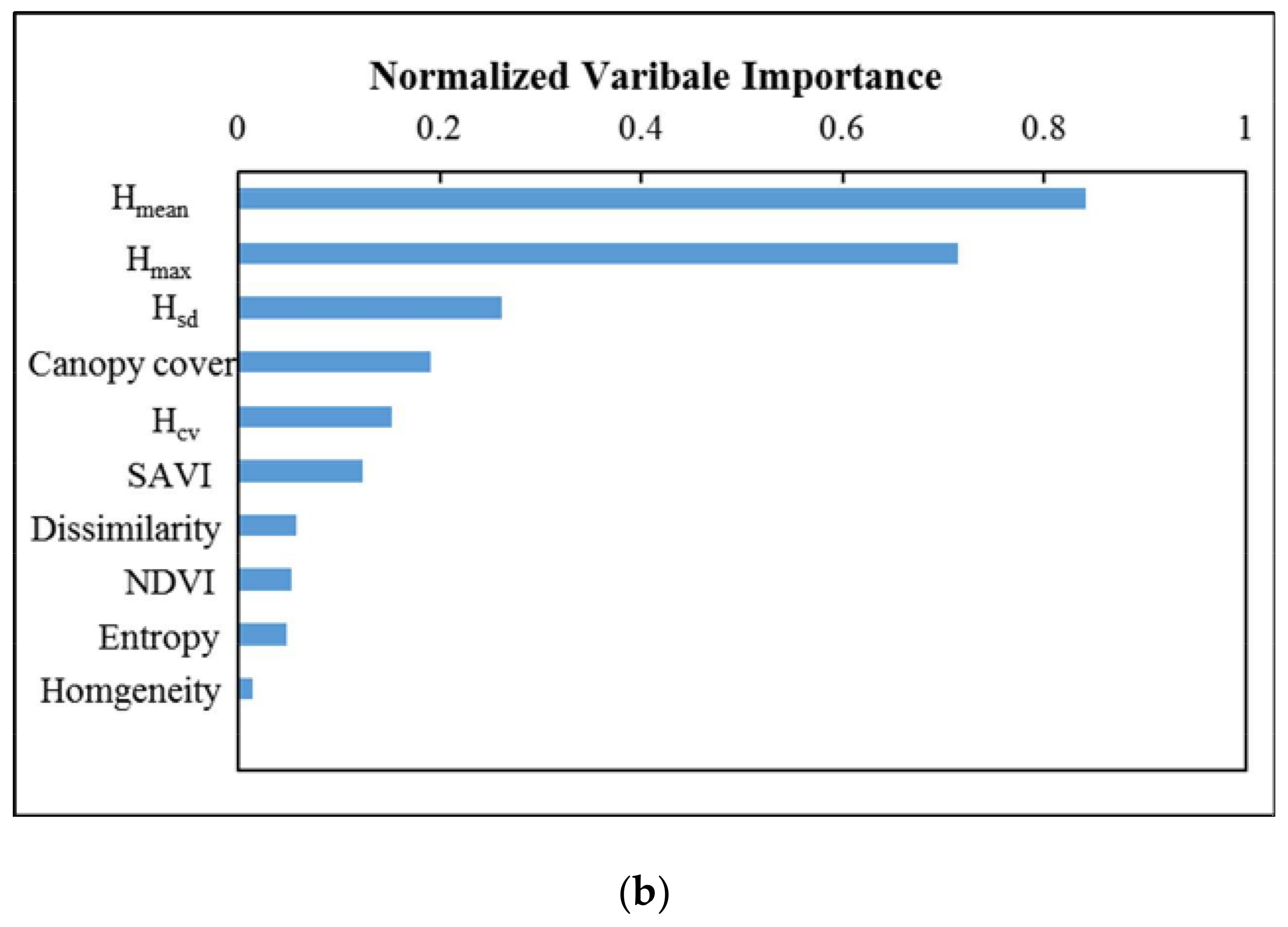
To summarize, this paper explores the best methods and the optimal combination of remote sensing data for forest AGB estimation. According to Figure 2, the best methods for estimating forest AGB are RF and an integration of LiDAR and optical data (OVs + TVs); these methods resulted in the best prediction model among the five input data combinations, i.e., OVs, LVs, OVs + LVs, OVs + TVs and LVs + TVs. We therefore used the best prediction model (based on LiDAR and optical data and the RF method) to generate a forest AGB map for the study area (Figure 5a). For this study, large areas show medium predicted biomass values, and higher biomass was mainly distributed in the southwest. The predicted forest aboveground biomass values were from 15.05 t/ha–207.6 t/ha, and many lower biomass values were concentrated in the northeast. Figure 5b presents that the higher predictor variables were used in the estimation, including Hmean, Hmax, Hsd, canopy cover, Hcv, SAVI, dissimilarity, NDVI, entropy and homogeneity ordered by normalized variable importance. The result showed that the Hmean and Hmax contributed greatly to the estimation, the normalized importance of which all exceeded 0.7. Comparing the data sources from which the predictor variables were derived, we found that LiDAR data contributed more to the forest estimation than optical data.
4. Discussion
In this paper, we compared model accuracies using single and integrated remote sensing data and five regression methods to estimate the forest AGB in arid and semi-arid regions of China. The results of the models revealed that the RF AGB model, which integrated LiDAR and optical variables, yielded the best estimation accuracy, with an R2 = 0.913 and RMSE = 13.352 t/ha. Therefore, it was essential to discuss the effects of predictive factors (data types, modeling methods and terrain data, etc.) for forest AGB model.
4.1. Importance of Predictive Factors for Model Performance
Previous studies revealed that the estimation accuracies of the models using different data types and modeling methods were various [34,65,66,67]. Therefore, it is essential to discuss the effect of data types and modeling methods on the forest biomass estimation. We used Analysis Of Variance (ANOVA) to rank the importance of the prediction methods and data types on the accuracy of forest AGB predictions (Table 4). In analysis results, the Sum of Squares values (SumSq) (which indicate an important contribution to the explained variance of R2 and RMSE) evaluated the importance of the predictive factors. Regarding variance in R2, the data types (SumSq = 0.082) seem to be more important than the prediction methods (SumSq = 0.065) for the accuracy of biomass prediction. ANOVA results for RMSE as the dependent variable showed that the SumSq of the predictor data types was high (1230.246), while the prediction method reached a relatively low SumSq (148.086). This indicates that the data type is more important than the modeling method for determining the model accuracy. The results are similar to those of an earlier study performed by Fassnacht et al. [33]; they found that data type was more important than prediction method and sample size in the forest biomass model.
4.1.1. Single vs. Integrated Data Sources for Estimating Forest AGB
In our study, the AGB models that used LiDAR data were better than optical data, and the results were similar to those of earlier findings [68,69]. Gobakken et al. [49] estimated forest biomass using airborne LiDAR data alone and obtained a very high accuracy (R2 = 0.95, RMSE = 19.02 t/ha) as a result. Kulawardhana et al. [69] indicated that LiDAR has a significantly higher predictive efficiency than optical data for estimating forest biomass. In related studies performed by Laurin et al. [23], it was found that the AGB model using optical data alone could limit prediction ability. This may be because optical data were generally disturbed by the saturation phenomenon in the region with signal saturation of high biomass or canopy density, and the AGB model accuracy was reduced. However, LiDAR data showed a close relationship with observed biomass and forest canopy structure under the same conditions. The combination of LiDAR and optical data can improve the accuracy of forest AGB estimation compared to the LiDAR-only model, to a certain degree, which is in line with previous studies [31,32]. The results from our study confirmed those findings, i.e., integrated LiDAR and optical data yielded the best results. The main reason is that optical data can provide complementary spectral information to LiDAR data, which offer 3D structural information about vegetation. The additional optical data improved R2 by 1.1%~6.2% compared with LiDAR data alone, which showed that incorporating optical data made a small contribution towards improving estimation accuracy. Predictor variables derived from LiDAR data were more important to biomass estimation than optical data according to Figure 5b. The relationships between biomass and the top two predictor variables (Hmean and Hmax) are shown in Figure 6. Hmean and Hmax were positively correlated with measured biomass; especially for Hmean, the R2 reached 0.721. As the important forest biophysical parameters, the height variables can effectively estimate the biomass due to the biomass of the branches and stems accounting for over 95% of the AGB for a mature forest [70]. Other researchers also found that the mean of the tree height was a good predictor factor for forest biomass estimation [71,72,73]. For example, Simard et al. [71] found that the mean tree height was highly related to the aboveground biomass in Everglades National Park. Scale is a crucial issue of the remote-sensing data; the resolution of optical data and the density of LiDAR point cloud have a strong effect on the forest biomass [74,75]. We will explore the effect of remote sensing data with different scales on biomass estimation accuracy in the future.
4.1.2. Influence of the Statistical Method on Estimation
The contribution of prediction methods is slightly smaller than that of data types according to the SumSq of R2, but its value is far less than data types in terms of RMSE. Among the considered methods, RF outperformed the other prediction methods, particularly when integrating LiDAR and optical data. The results of the GLMM AGB model are unstable with a relatively higher R2 and RMSE. SVM performed more poorly than the tested models, and the performances of the BPNN and KNN methods were always the worst. Fassnacht et al. [25] compared the accuracy of the forest AGB model that used RF, KNN, SVM, LMSTEP (Stepwise Linear Models) and GP (Gaussian Processes) and found that RF was the best method used for prediction. The RF method was also used by Liu et al. [26], and they found that RF was a better method than Stepwise Regression (SR) and SVM, when estimating forest AGB in Heilongjiang Province of China. Our study corroborated these research works; the RF method was able to use different kinds of data for forest biomass estimation, and the prediction result is more optimal than these general methods. The RF method performed very well compared to many other regressions, which may be due to the fact that each node in the random forest is split using the best among a subset of predictors randomly chosen at that node [76]. In this study, we only systematically compared five common modeling methods (RF, SVM, BPNN, KNN and GLMM), but the model has its own disadvantage in different degrees. The algorithms themselves can be further researched, and we will explore the integrated modeling method with the advantages of each algorithm.
4.2. Impact of Sample Size on Forest AGB Estimation
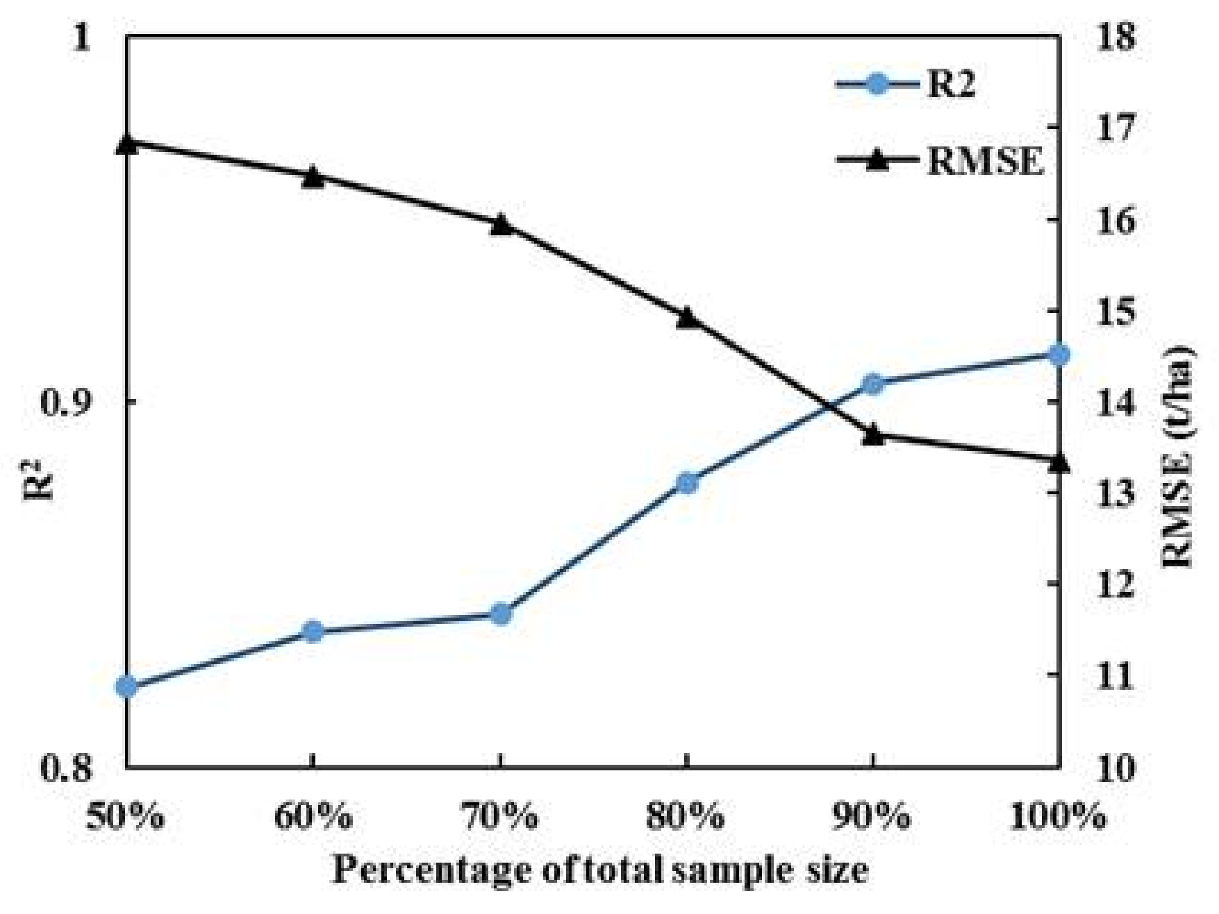
A large number of sample plots in forest inventories is costly; however, sample size has an effect on the precision of forest biomass estimation [77]. Therefore, it is necessary to explore the impact of sample size on the prediction model and improve the sampling efficiency and prediction accuracy. The modeling accuracy results of RF AGB models estimated with different sample sizes (50%, 60%, 70%, 80%, 90% and 100% of measured biomass) are shown in Figure 7. It is indicated that the R2 is increasing and RMSE decreasing with the increase of the sample size; however, the range of variation slows when the sample size to be more than 90%. This appears similar to Jacob et al. [30,78]; they analyzed the effects of various LiDAR pulse densities and sample sizes on a model-assisted approach to estimate forest inventory variables. The result showed that model accuracy was hardly increasing when the number was more than 35. In the previous studies, Fassnacht et al. [33] reviewed studies with regard to the number of sample sizes and remote sensing data used in the forest biomass estimation. They have explored relevant studies from 2000–2013 and found a sample size between 20 and 50 in most studies, especially for 30. Nie and Luo et al. [30,51] have used airborne LiDAR data and 33 plots’ measurement data to estimate the forest AGB and achieved better prediction results (R2 = 0.815 and 0.893, respectively). Their study regions were similar to ours, which were located on Heihe River Basin in arid and semi-arid regions of China. These research works indicated that the prediction model is achievable in our study, which also may be due to the sample plot being typical. Compared to the number of sample sizes, the distribution of the sample plots was also important for the prediction model [79]. The optimal distribution of the sample plots could, to a certain extent, compensate for reducing the number of sample sizes [80]. Even though the number of field sample plots (32 sample plots) is not abundant, we think that the prediction results are valid under the area with a simple forest landscape in our study.
4.3. Effect of Terrain Variables on the Prediction Model
Our second-best model for AGB is the RF method that integrated LiDAR and terrain data; it indicated that terrain data can contribute similar information as optical data. The results suggest that terrain data may be sufficient to improving the accuracy of forest AGB estimation. This agrees with the result found by Mohamedou et al. [56]; they concluded that the terrain data demonstrate usefulness in improving prediction accuracy for tree growth in southeast Finland. Similar research results were found by Claudia et al. [81]; they used GLAS data to estimate forest height and found that the estimation was influenced by surface topography. Greaves et al. [57] found that the model accuracy of shrub biomass was improved with additional terrain data, and they considered that both optical and terrain data improved biomass prediction may be due to LiDAR point clouds that cannot capture the structure of vegetation in areas with low biomass. The positive effect of terrain data for forest biomass estimation was possibly due to the fact that the area of our study had a rough topography with steep slopes and deep valleys. Further studies are required to explore the contributions of terrain variables in estimating forest biomass under various topographical conditions and to develop applicative methods for retrieving forest biomass in different regions, such as study areas with similar topographic conditions.
5. Conclusions
In this study, we compared the prediction accuracy of various data types and modeling methods for estimating forest AGB. The results indicated that RF is the best modeling method, no matter the types of datasets. However, for the RF AGB model, the results from the five input datasets were different. LiDAR data were more effective than optical data for estimating forest AGB, and incorporating additional terrain variables could slightly improve the estimation accuracy. The optimal AGB model, which used the RF method with integrated airborne LiDAR and optical data, mapped at the regional scale over the Upper Heihe River Basin in Northwest China.
Our work was a modest contribution to the study of using the combination of LiDAR and optical data to estimate forest biomass in arid and semi-arid regions. However, the utilization of LiDAR was limited by the relatively small coverage, which led to a low ability to generalize the prediction methods for different forest structure distribution areas. This requires extensive field and remote sensing data to improve statistics and establish a link between regional and global-scale biomass information. Further research is particularly important to focus on areas with special climate conditions, such as topical forests and water conservation forests, in arid and semi-arid regions.
Acknowledgments
This work is supported by the national Natural Science Foundation of China (Nos. 41171173 and 40771089) and the Priority Academic Program Development of the Jiangsu Higher Education Institutions (PAPD). The authors would like to express our appreciation to Heihe Plan Science Data Center for the support of the data. We would also like to express our thanks to the anonymous reviewers for providing useful comments to improve the paper.
Author Contributions
Luodan Cao designed the framework of this research work and wrote the manuscript. Jianjun Pan proposed the main idea and provided important guidance on the work. Ruijuan Li performed the experiments. Jialin Li gave guidance on this work, and Zhaofu Li checked the writing.
Conflicts of Interest
The authors declare no conflict of interest.
References
- Houghton, R.A.; Hall, F.; Goetz, S.J. Importance of biomass in the global carbon cycle. J. Geophys. Res. Biogeosci. 2009, 114, 13. [Google Scholar] [CrossRef]
- Canadell, J.G.; Le Quere, C.; Raupach, M.R.; Field, C.B.; Buitenhuis, E.T.; Ciais, P.; Conway, T.J.; Gillett, N.P.; Houghton, R.A.; Marland, G. Contributions to accelerating atmospheric CO2 growth from economic activity, carbon intensity, and efficiency of natural sinks. Proc. Natl. Acad. Sci. USA 2007, 104, 18866–18870. [Google Scholar] [CrossRef] [PubMed] [Green Version]
- Gibbs, H.K.; Brown, S.; Niles, J.O.; Foley, J.A. Monitoring and estimating tropical forest carbon stocks: Making REDD a reality. Environ. Res. Lett. 2007, 2, 13. [Google Scholar] [CrossRef]
- Saatchi, S.S.; Harris, N.L.; Brown, S.; Lefsky, M.; Mitchard, E.T.A.; Salas, W.; Zutta, B.R.; Buermann, W.; Lewis, S.L.; Hagen, S.; et al. Benchmark map of forest carbon stocks in tropical regions across three continents. Proc. Natl. Acad. Sci. USA 2011, 108, 9899–9904. [Google Scholar] [CrossRef] [PubMed]
- Ene, L.T.; Naesset, E.; Gobakken, T.; Gregoire, T.G.; Stahl, G.; Holm, S. A simulation approach for accuracy assessment of two-phase post-stratified estimation in large-area LiDAR biomass surveys. Remote Sens. Environ. 2013, 133, 210–224. [Google Scholar] [CrossRef]
- Ahmed, R.; Siqueira, P.; Hensley, S. A study of forest biomass estimates from LiDAR in the northern temperate forests of New England. Remote Sens. Environ. 2013, 130, 121–135. [Google Scholar] [CrossRef]
- Ene, L.T.; Naesset, E.; Gobakken, T.; Gregoire, T.G.; Stahl, G.; Nelson, R. Assessing the accuracy of regional LiDAR-based biomass estimation using a simulation approach. Remote Sens. Environ. 2012, 123, 579–592. [Google Scholar] [CrossRef]
- Ioki, K.; Tsuyuki, S.; Hirata, Y.; Phua, M.H.; Wong, W.V.C.; Ling, Z.Y.; Saito, H.; Takao, G. Estimating above-ground biomass of tropical rainforest of different degradation levels in Northern Borneo using airborne LiDAR. For. Ecol. Manag. 2014, 328, 335–341. [Google Scholar] [CrossRef]
- Pflugmacher, D.; Cohen, W.B.; Kennedy, R.E.; Yang, Z.Q. Using Landsat-derived disturbance and recovery history and LiDAR to map forest biomass dynamics. Remote Sens. Environ. 2014, 151, 124–137. [Google Scholar] [CrossRef]
- Lin, Y.; West, G. Reflecting conifer phenology using mobile terrestrial LiDAR: A case study of Pinus sylvestris growing under the Mediterranean climate in Perth, Australia. Ecol. Indic. 2016, 70, 1–9. [Google Scholar] [CrossRef]
- Huete, A.; Justice, C.; Liu, H. Development of vegetation and soil indexes for MODIS-EOS. Remote Sens. Environ. 1994, 49, 224–234. [Google Scholar] [CrossRef]
- Blackard, J.A.; Finco, M.V.; Helmer, E.H.; Holden, G.R.; Hoppus, M.L.; Jacobs, D.M.; Lister, A.J.; Moisen, G.G.; Nelson, M.D.; Riemann, R.; et al. Mapping us forest biomass using nationwide forest inventory data and moderate resolution information. Remote Sens. Environ. 2008, 112, 1658–1677. [Google Scholar] [CrossRef]
- Foody, G.M.; Boyd, D.S.; Cutler, M.E.J. Predictive relations of tropical forest biomass from Landsat TM data and their transferability between regions. Remote Sens. Environ. 2003, 85, 463–474. [Google Scholar] [CrossRef]
- Pu, R.L.; Cheng, J. Mapping forest leaf area index using reflectance and textural information derived from worldview-2 imagery in a mixed natural forest area in Florida, US. Int. J. Appl. Earth Obs. Geoinf. 2015, 42, 11–23. [Google Scholar] [CrossRef]
- Avitabile, V.; Baccini, A.; Friedl, M.A.; Schmullius, C. Capabilities and limitations of Landsat and land cover data for aboveground woody biomass estimation of Uganda. Remote Sens. Environ. 2012, 117, 366–380. [Google Scholar] [CrossRef]
- Gao, M.L.; Zhao, W.J.; Gong, Z.N.; Gong, H.L.; Chen, Z.; Tang, X.M. Topographic correction of ZY-3 satellite images and its effects on estimation of shrub leaf biomass in mountainous areas. Remote Sens. 2014, 6, 2745–2764. [Google Scholar] [CrossRef]
- Chi, H.; Sun, G.Q.; Huang, J.L.; Guo, Z.F.; Ni, W.J.; Fu, A.M. National forest aboveground biomass mapping from ICESat/GLAS data and MODIS imagery in China. Remote Sens. 2015, 7, 5534–5564. [Google Scholar] [CrossRef]
- Kumar, L.; Mutanga, O. Remote sensing of above-ground biomass. Remote Sens. 2017, 9, 935. [Google Scholar] [CrossRef]
- Ni, W.; Sun, G.; Ranson, K.J.; Pang, Y.; Zhang, Z.; Yao, W. Extraction of ground surface elevation from ZY-3 winter stereo imagery over deciduous forested areas. Remote Sens. Environ. 2015, 159, 194–202. [Google Scholar] [CrossRef]
- Sun, G.; Ni, W.; Zhang, Z.; Xiong, C. Forest abovegroundbiomass mapping using spaceborne stereo imagery acquired by Chinese ZY-3. In Proceedings of the AGU Fall Meeting, San Francisco, CA, USA, 14–18 December 2015; Volume 12, p. 2089. [Google Scholar]
- Santi, E.; Paloscia, S.; Pettinato, S.; Fontanelli, G.; Mura, M.; Zolli, C.; Maselli, F.; Chiesi, M.; Bottai, L.; Chirici, G. The potential of multifrequency SAR images for estimating forest biomass in Mediterranean areas. Remote Sens. Environ. 2017, 200, 63–73. [Google Scholar] [CrossRef]
- Zhou, T.; Li, Z.; Pan, J. Multi-feature classification of multi-sensor satellite imagery based on dual-polarimetric Sentinel-1a, Landsat-8 oli, and hyperion images for urban land-cover classification. Sensors 2018, 18, 373. [Google Scholar] [CrossRef] [PubMed]
- Laurin, G.V.; Chen, Q.; Lindsell, J.A.; Coomes, D.A.; Del Frate, F.; Guerriero, L.; Pirotti, F.; Valentini, R. Above ground biomass estimation in an African tropical forest with LiDAR and hyperspectral data. ISPRS-J. Photogramm. Remote Sens. 2014, 89, 49–58. [Google Scholar] [CrossRef]
- He, Q.S.; Chen, E.X.; An, R.; Li, Y. Above-ground biomass and biomass components estimation using LiDAR data in a coniferous forest. Forests 2013, 4, 984–1002. [Google Scholar] [CrossRef]
- Singh, K.K.; Chen, G.; Vogler, J.B.; Meentemeyer, R.K. When big data are too much: Effects of LiDAR returns and point density on estimation of forest biomass. IEEE J. Sel. Top. Appl. Earth Obs. Remote Sens. 2016, 9, 3210–3218. [Google Scholar] [CrossRef]
- Lefsky, M.A.; Cohen, W.B.; Parker, G.G.; Harding, D.J. LiDAR remote sensing for ecosystem studies. Bioscience 2002, 52, 19–30. [Google Scholar] [CrossRef]
- Zolkos, S.G.; Goetz, S.J.; Dubayah, R. A meta-analysis of terrestrial aboveground biomass estimation using LiDAR remote sensing. Remote Sens. Environ. 2013, 128, 289–298. [Google Scholar] [CrossRef]
- Su, Y.J.; Guo, Q.H.; Xue, B.L.; Hu, T.Y.; Alvarez, O.; Tao, S.L.; Fang, J.Y. Spatial distribution of forest aboveground biomass in China: Estimation through combination of spaceborne LiDAR, optical imagery, and forest inventory data. Remote Sens. Environ. 2016, 173, 187–199. [Google Scholar] [CrossRef]
- Chi, H.; Sun, G.Q.; Huang, J.L.; Li, R.D.; Ren, X.Y.; Ni, W.J.; Fu, A.M. Estimation of forest aboveground biomass in Changbai mountain region using ICESat/GLAS and Landsat/TM data. Remote Sens. 2017, 9, 707. [Google Scholar] [CrossRef]
- Luo, S.Z.; Wang, C.; Xi, X.H.; Pan, F.F.; Peng, D.L.; Zou, J.; Nie, S.; Qin, H.M. Fusion of airborne LiDAR data and hyperspectral imagery for aboveground and belowground forest biomass estimation. Ecol. Indic. 2017, 73, 378–387. [Google Scholar] [CrossRef]
- Brovkina, O.; Novotny, J.; Cienciala, E.; Zemek, F.; Russ, R. Mapping forest aboveground biomass using airborne hyperspectral and LiDAR data in the mountainous conditions of central Europe. Ecol. Eng. 2017, 100, 219–230. [Google Scholar] [CrossRef]
- Swatantran, A.; Dubayah, R.; Roberts, D.; Hofton, M.; Blair, J.B. Mapping biomass and stress in the Sierra Nevada using LiDAR and hyperspectral data fusion. Remote Sens. Environ. 2011, 115, 2917–2930. [Google Scholar] [CrossRef]
- Fassnacht, F.E.; Hartig, F.; Latifi, H.; Berger, C.; Hernandez, J.; Corvalan, P.; Koch, B. Importance of sample size, data type and prediction method for remote sensing-based estimations of aboveground forest biomass. Remote Sens. Environ. 2014, 154, 102–114. [Google Scholar] [CrossRef]
- Liu, K.; Wang, J.; Zeng, W.; Song, J. Comparison and evaluation of three methods for estimating forest above ground biomass using TM and GLAS data. Remote Sens. 2017, 9, 341. [Google Scholar] [CrossRef]
- Shao, Z.; Zhang, L. Estimating forest aboveground biomass by combining optical and SAR data: A case study in Genhe, Inner Mongolia, China. Sensors 2016, 16, 834. [Google Scholar] [CrossRef] [PubMed]
- De Toledo, J.J.; Magnusson, W.E.; Castilho, C.V.; Nascimento, H.E.M. Tree mode of death in central Amazonia: Effects of soil and topography on tree mortality associated with storm disturbances. For. Ecol. Manag. 2012, 263, 253–261. [Google Scholar] [CrossRef]
- Ferry, B.; Morneau, F.; Bontemps, J.-D.; Blanc, L.; Freycon, V. Higher treefall rates on slopes and waterlogged soils result in lower stand biomass and productivity in a tropical rain forest. J. Ecol. 2010, 98, 106–116. [Google Scholar] [CrossRef]
- Singh, K.K.; Bianchetti, R.A.; Chen, G.; Meentemeyer, R.K. Assessing effect of dominant land-cover types and pattern on urban forest biomass estimated using LiDAR metrics. Urban Ecosyst. 2017, 20, 265–275. [Google Scholar] [CrossRef]
- Viana, H.; Aranha, J.; Lopes, D.; Cohen, W.B. Estimation of crown biomass of Pinus pinaster stands and shrubland above-ground biomass using forest inventory data, remotely sensed imagery and spatial prediction models. Ecol. Model. 2012, 226, 22–35. [Google Scholar] [CrossRef]
- Lee, I.S.; Ge, L.L. The performance of RTK-GPS for surveying under challenging environmental conditions. Earth Planets Space 2006, 58, 515–522. [Google Scholar] [CrossRef]
- Wang, J.; Ju, K.; Fu, H.; Chang, X. Study on biomass of water conservation forest on North Slope of Qilian Mountains. J. Fujian Coll. For. 1998, 18, 319–323. [Google Scholar]
- Xiao, Q.; Wen, J. HIWATER: Airborne LiDAR Raw Data in Tianlaochi Catchment; Heihe Plan Science Data Center: Heihe, China, 2014. [Google Scholar]
- Qi, J.; Chehbouni, A.; Huete, A.R.; Kerr, Y.H.; Sorooshian, S. A modified soil adjusted vegetation index. Remote Sens. Environ. 1994, 48, 119–126. [Google Scholar] [CrossRef]
- Rondeaux, G.; Steven, M.; Baret, F. Optimization of soil-adjusted vegetation indices. Remote Sens. Environ. 1996, 55, 95–107. [Google Scholar] [CrossRef]
- Mutanga, O.; Skidmore, A.K. Narrow band vegetation indices overcome the saturation problem in biomass estimation. Int. J. Remote Sens. 2004, 25, 3999–4014. [Google Scholar] [CrossRef]
- Liu, D.; Pu, H.B.; Sun, D.W.; Wang, L.; Zeng, X.A. Combination of spectra and texture data of hyperspectral imaging for prediction of pH in salted meat. Food Chem. 2014, 160, 330–337. [Google Scholar] [CrossRef] [PubMed]
- Wulder, M.A.; LeDrew, E.F.; Franklin, S.E.; Lavigne, M.B. Aerial image texture information in the estimation of northern deciduous and mixed wood forest leaf area index (LAI). Remote Sens. Environ. 1998, 64, 64–76. [Google Scholar] [CrossRef]
- Pan, J.P.; Gong, J.Y.; Lu, J.; Ye, H.Z.; Chen, X.L.; Yang, J.L. Classification based on texture feature of wavelet transform. In Instruments, Science, and Methods for Geospace and Planetary Remote Sensing; Nardell, C.A., Lucey, P.G., Yee, J.H., Garvin, J.B., Eds.; SPIE: Bellingham, WA, USA, 2004; Volume 5660, pp. 208–217. [Google Scholar]
- Frazer, G.W.; Magnussen, S.; Wulder, M.A.; Niemann, K.O. Simulated impact of sample plot size and co-registration error on the accuracy and uncertainty of LiDAR-derived estimates of forest stand biomass. Remote Sens. Environ. 2011, 115, 636–649. [Google Scholar] [CrossRef]
- Dubayah, R.O.; Sheldon, S.L.; Clark, D.B.; Hofton, M.A.; Blair, J.B.; Hurtt, G.C.; Chazdon, R.L. Estimation of tropical forest height and biomass dynamics using LiDAR remote sensing at La Selva, Costa Rica. J. Geophys. Res. Biogeosci. 2010, 115. [Google Scholar] [CrossRef]
- Nie, S.; Wang, C.; Zeng, H.C.; Xi, X.H.; Li, G.C. Above-ground biomass estimation using airborne discrete-return and full-waveform LiDAR data in a coniferous forest. Ecol. Indic. 2017, 78, 221–228. [Google Scholar] [CrossRef]
- Lang, M.W.; McCarty, G.W. LiDAR intensity for improved detection of inundation below the forest canopy. Wetlands 2009, 29, 1166–1178. [Google Scholar] [CrossRef]
- Ni-Meister, W.; Lee, S.Y.; Strahler, A.H.; Woodcock, C.E.; Schaaf, C.; Yao, T.A.; Ranson, K.J.; Sun, G.Q.; Blair, J.B. Assessing general relationships between aboveground biomass and vegetation structure parameters for improved carbon estimate from LiDAR remote sensing. J. Geophys. Res. Biogeosci. 2010, 115, 12. [Google Scholar] [CrossRef]
- Korhonen, L.; Korpela, I.; Heiskanen, J.; Maltamo, M. Airborne discrete-return LiDAR data in the estimation of vertical canopy cover, angular canopy closure and leaf area index. Remote Sens. Environ. 2011, 115, 1065–1080. [Google Scholar] [CrossRef]
- Zhang, G.; Ganguly, S.; Nemani, R.R.; White, M.A.; Milesi, C.; Hashimoto, H.; Wang, W.L.; Saatchi, S.; Yu, Y.F.; Myneni, R.B. Estimation of forest aboveground biomass in California using canopy height and leaf area index estimated from satellite data. Remote Sens. Environ. 2014, 151, 44–56. [Google Scholar] [CrossRef]
- Jensen, J.L.R.; Mathews, A.J. Assessment of image-based point cloud products to generate a bare earth surface and estimate canopy heights in a woodland ecosystem. Remote Sens. 2016, 8, 50. [Google Scholar] [CrossRef]
- Glenn, N.F.; Streutker, D.R.; Chadwick, D.J.; Thackray, G.D.; Dorsch, S.J. Analysis of LiDAR-derived topographic information for characterizing and differentiating landslide morphology and activity. Geomorphology 2006, 73, 131–148. [Google Scholar] [CrossRef]
- O’Loughlin, E.J.; Chin, Y.P. Quantification and characterization of dissolved organic carbon and iron in sedimentary porewater from green bay, WI, USA. Biogeochemistry 2004, 71, 371–386. [Google Scholar] [CrossRef]
- Karlson, M.; Ostwald, M.; Reese, H.; Sanou, J.; Tankoano, B.; Mattsson, E. Mapping tree canopy cover and aboveground biomass in Sudano-Sahelian woodlands using Landsat 8 and random forest. Remote Sens. 2015, 7, 10017–10041. [Google Scholar] [CrossRef]
- Mountrakis, G.; Im, J.; Ogole, C. Support vector machines in remote sensing: A review. ISPRS-J. Photogramm. Remote Sens. 2011, 66, 247–259. [Google Scholar] [CrossRef]
- Wang, L.; Zeng, Y.; Chen, T. Back propagation neural network with adaptive differential evolution algorithm for time series forecasting. Expert Syst. Appl. 2015, 42, 855–863. [Google Scholar] [CrossRef]
- Pandya, D.H.; Upadhyay, S.H.; Harsha, S.P. Fault diagnosis of rolling element bearing with intrinsic mode function of acoustic emission data using APF-KNN. Expert Syst. Appl. 2013, 40, 4137–4145. [Google Scholar] [CrossRef]
- Preacher, K.J.; Curran, P.J.; Bauer, D.J. Computational tools for probing interactions in multiple linear regression, multilevel modeling, and latent curve analysis. J. Educ. Behav. Stat. 2006, 31, 437–448. [Google Scholar] [CrossRef]
- Martinez, B.; Garcia-Haro, F.J.; Camacho-de Coca, F. Derivation of high-resolution leaf area index maps in support of validation activities: Application to the cropland Barrax site. Agric. For. Meteorol. 2009, 149, 130–145. [Google Scholar] [CrossRef]
- Fang, J.Y.; Wang, Z.M. Forest biomass estimation at regional and global levels, with special reference to China’s forest biomass. Ecol. Res. 2001, 16, 587–592. [Google Scholar] [CrossRef]
- Xing, Y.-Q.; Wang, L.-H. Compatible biomass estimation models of natural forests in Changbai Mountains based on forest inventory. Yingyong Shengtai Xuebao 2007, 18, 1–8. [Google Scholar] [PubMed]
- Ahmed, R.; Siqueira, P.; Hensley, S.; Bergen, K. Uncertainty of forest biomass estimates in north temperate forests due to allometry: Implications for remote sensing. Remote Sens. 2013, 5, 3007–3036. [Google Scholar] [CrossRef]
- Gobakken, T.; Naesset, E.; Nelson, R.; Bollandsas, O.M.; Gregoire, T.G.; Stahl, G.; Holm, S.; Orka, H.O.; Astrup, R. Estimating biomass in Hedmark County, Norway using national forest inventory field plots and airborne laser scanning. Remote Sens. Environ. 2012, 123, 443–456. [Google Scholar] [CrossRef]
- Kulawardhana, R.W.; Popescu, S.C.; Feagin, R.A. Fusion of LiDAR and multispectral data to quantify salt marsh carbon stocks. Remote Sens. Environ. 2014, 154, 345–357. [Google Scholar] [CrossRef]
- Kenzo, T.; Furutani, R.; Hattori, D.; Tanaka, S.; Sakurai, K.; Ninomiya, I.; Kendawang, J.J. Aboveground and belowground biomass in logged-over tropical rain forests under different soil conditions in borneo. J. For. Res. 2015, 20, 197–205. [Google Scholar] [CrossRef]
- Simard, M.; Zhang, K.; Rivera-Monroy, V.H.; Ross, M.S.; Ruiz, P.L.; Castañeda-Moya, E.; Twilley, R.R.; Rodriguez, E. Mapping height and biomass of mangrove forests in Everglades National Park with SRTM elevation data. Photogramm. Eng. Remote Sens. 2006, 72, 299–311. [Google Scholar] [CrossRef]
- Lefsky, M.A.; Cohen, W.B.; Harding, D.J.; Parker, G.G.; Acker, S.A.; Gower, S.T. Lidar remote sensing of above-ground biomass in three biomes. Glob. Ecol. Biogeogr. Lett. 2002, 11, 393–399. [Google Scholar] [CrossRef]
- Lefsky, M.A.; Harding, D.; Cohen, W.B.; Parker, G.; Shugart, H.H. Surface LiDAR remote sensing of basal area and biomass in deciduous forests of Eastern Maryland, USA. Remote Sens. Environ. 1999, 67, 83–98. [Google Scholar]
- Chen, G.; Ozelkan, E.; Singh, K.K.; Zhou, J.; Brown, M.R.; Meentemeyer, R.K. Uncertainties in mapping forest carbon in urban ecosystems. J. Environ. Manag. 2017, 187, 229–238. [Google Scholar] [CrossRef] [PubMed]
- Gu, H.; Townsend, P.A. Mapping forest structure and uncertainty in an urban area using leaf-off LiDAR data. Urban Ecosyst. 2017, 20, 497–509. [Google Scholar] [CrossRef]
- Hultquist, C.; Chen, G.; Zhao, K. A comparison of Gaussian process regression, random forests and support vector regression for burn severity assessment in diseased forests. Remote Sens. Lett. 2014, 5, 723–732. [Google Scholar] [CrossRef]
- Gobakken, T.; Naesset, E. Assessing effects of laser point density, ground sampling intensity, and field sample plot size on biophysical stand properties derived from airborne laser scanner data. Can. J. For. Res.-Rev. Can. Rech. For. 2008, 38, 1095–1109. [Google Scholar] [CrossRef]
- Strunk, J.; Temesgen, H.; Andersen, H.-E.; Flewelling, J.P.; Madsen, L. Effects of LiDAR pulse density and sample size on a model-assisted approach to estimate forest inventory variables. Can. J. Remote Sens. 2012, 38, 644–654. [Google Scholar] [CrossRef]
- Paine, C.E.T.; Baraloto, C.; Diaz, S. Optimal strategies for sampling functional traits in species-rich forests. Funct. Ecol. 2015, 29, 1325–1331. [Google Scholar] [CrossRef]
- Gutjahr, A. Geostatistics for sampling designs and analysis. ACS Symp. Ser. 1990, 465, 48–90. [Google Scholar]
- Hilbert, C.; Schmullius, C. Influence of surface topography on ICESat/GLAS forest height estimation and waveform shape. Remote Sens. 2012, 4, 2210–2235. [Google Scholar] [CrossRef]
Figure 1.
The spatial distribution of land use type and sample plots in our study area.

Figure 2.
The boxplots illustrate model accuracy results using different input datasets and prediction methods: The distribution of the mean R2 (a) and the mean RMSE (b) from the 50 bootstrapped models obtained using the five-fold-cross-validation for each prediction method. The black dotted lines represent the mean value. RF, Random Forest; SVM, Support Vector Machines; BPNN, Back Propagation Neural Networks; KNN, K-Nearest Neighbor; GLMM, Generalized Linear Mixed Model; OVs, optical variables; LVs, LiDAR variables; OVs + LVs, the combination of optical and LiDAR variables, OVs + TVs, the combination of optical and terrain variables; LVs + TVs, the combination of LiDAR and terrain variables.

Figure 3.
The mean R2 and RMSE of AGB models, which used five methods based on different datasets. RF, Random Forest; SVM, Support Vector Machines; BPNN, Back Propagation Neural Networks; KNN, K-Nearest Neighbor; GLMM, Generalized Linear Mixed Model; OVs, optical variables; LVs, LiDAR variables; OVs + LVs, the combination of optical and LiDAR variables, OVs + TVs, the combination of optical and terrain variables; LVs + TVs, the combination of LiDAR and terrain variables.
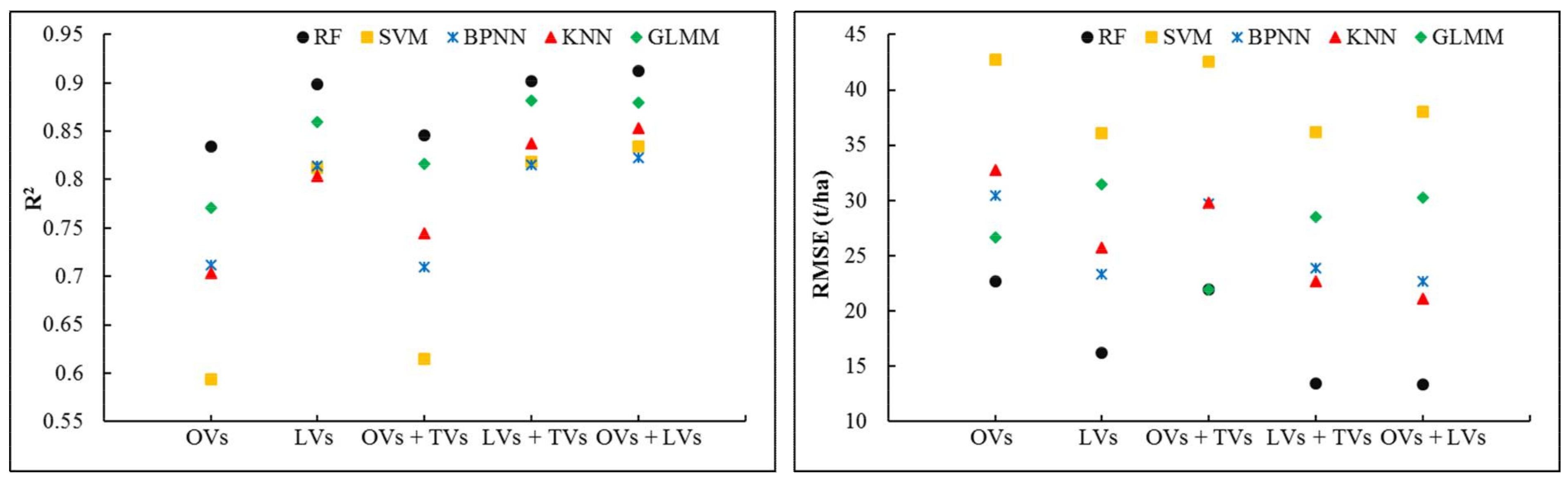
Figure 4.
Predicted AGB vs. measured AGB. The black dotted line represents the 1:1 line. RF, Random Forest; SVM, Support Vector Machines; BPNN, Back Propagation Neural Networks; KNN, K-Nearest Neighbor; GLMM, Generalized Linear Mixed Model.
Figure 4.
Predicted AGB vs. measured AGB. The black dotted line represents the 1:1 line. RF, Random Forest; SVM, Support Vector Machines; BPNN, Back Propagation Neural Networks; KNN, K-Nearest Neighbor; GLMM, Generalized Linear Mixed Model.

Figure 5.
(a) Map of the mean biomass estimates as obtained from the 50 bootstrapped model runs, using the LiDAR and optical data variables in the random forest model; (b) the important contributions of different predictor variables were used in the estimation.
Figure 5.
(a) Map of the mean biomass estimates as obtained from the 50 bootstrapped model runs, using the LiDAR and optical data variables in the random forest model; (b) the important contributions of different predictor variables were used in the estimation.
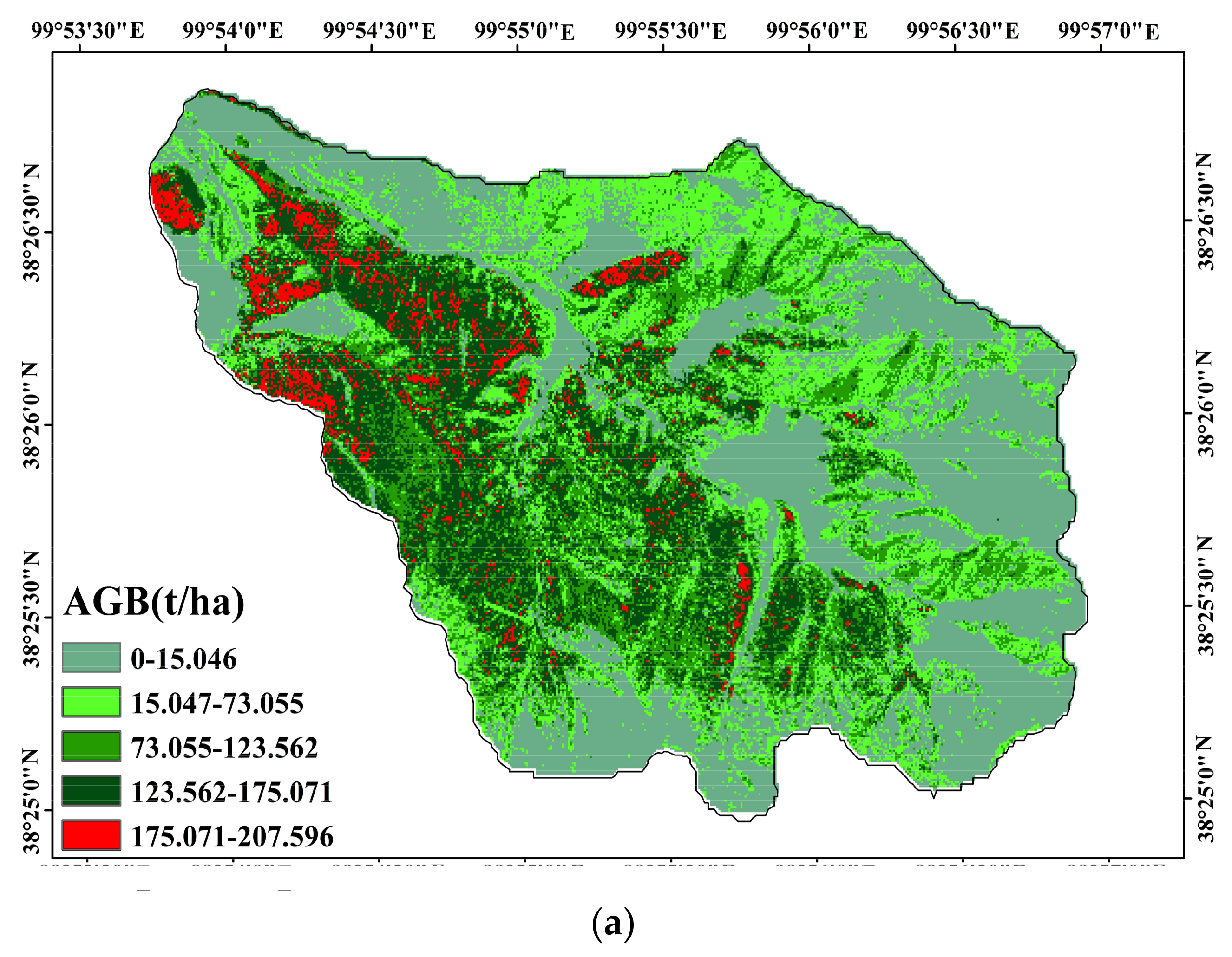

Figure 6.
Measured aboveground biomass versus the mean (a) and the max (b) of tree height in the sample plot.
Figure 6.
Measured aboveground biomass versus the mean (a) and the max (b) of tree height in the sample plot.
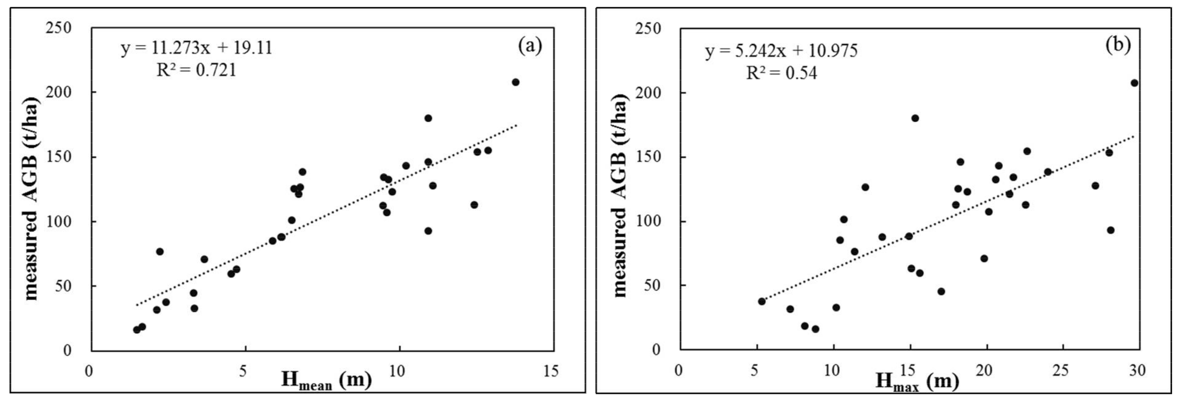
Figure 7.
Accuracies of the RF AGB models estimated by different sample sizes.


Table 1.
Vegetation indices and equations used in this study.
| Variables | Equations | Description |
|---|---|---|
| Ratio Vegetation Index (RVI) | bandNir/bandR | Reduces the effects of atmosphere and topography |
| Normalized Difference Index (NDVI) | (bandNir − bandR)/(bandNir + bandR) | Enhances the responsiveness to the vegetation |
| Soil-Adjusted Vegetation Index (SAVI) | The value of L can be automatically adjusted following the density of the vegetation | |
| Modified Soil-Adjusted Vegetation Index (MSAVI) | Reduces the disturbances of soil background |
Table 2.
Summary of the LiDAR features extraction used in this study.
| Metric ID | Metric | Description |
|---|---|---|
| LiDAR-derived variables | Hmax | Maximum of LiDAR height |
| Hmean | Mean of LiDAR height | |
| HSD | Standard deviation of LiDAR height | |
| HCV | Coefficient of variation of LiDAR height | |
| Canopy cover (Cc) | Canopy cover derived from LiDAR returns number | |
| Terrain variables | Topographic Wetness Index (TWI) | Reflects the condition of soil |
| Hillshade | Generalized directional topographic exposure | |
| Profile Curvature (PC) | Describes variation of slope | |
| Slope | Reflects tilt of local topography |
Table 3.
The packages and parameters of five methods used in the R.
| Methods | Package | Parameters |
|---|---|---|
| Random Forest (RF) | ‘randomforest’ | Ntree with 500 and mtry with 25 |
| Support Vector Machines (SVM) | ‘kernlab’ | Penalty factor with 2^(−6:2) and kernel parameters with 2^(−4:4) |
| Back Propagational Neural Networks (BPNN) | ‘amore’ | Number of iterations with 16 |
| K-Nearest Neighbor (KNN) | ‘knn’ | Number of adjacent sample sizes, which was set from 2 to 5 |
| Generalized Linear Mixed Model (GLMM) | ‘lme4’ | Logistic regression function was used and the growth parameter with 0.2 |
Table 4.
Results of ANOVA conducted to explain the variance of R2 and RMSE obtained for the different experiments. SumSq, Sum of Squares.
Table 4.
Results of ANOVA conducted to explain the variance of R2 and RMSE obtained for the different experiments. SumSq, Sum of Squares.
| Response Variable | df | R2 | RMSE | ||||
|---|---|---|---|---|---|---|---|
| SumSq | F | Sig. | SumSq | F | Sig. | ||
| Data types | 4 | 0.082 | 17.603 | 0.000 | 1230.246 | 25.513 | 0.000 |
| Methods | 4 | 0.065 | 13.798 | 0.000 | 148.086 | 3.071 | 0.047 |
© 2018 by the authors. Licensee MDPI, Basel, Switzerland. This article is an open access article distributed under the terms and conditions of the Creative Commons Attribution (CC BY) license (http://creativecommons.org/licenses/by/4.0/).
Share and Cite
MDPI and ACS Style
Cao, L.; Pan, J.; Li, R.; Li, J.; Li, Z. Integrating Airborne LiDAR and Optical Data to Estimate Forest Aboveground Biomass in Arid and Semi-Arid Regions of China. Remote Sens. 2018, 10, 532. https://doi.org/10.3390/rs10040532
AMA Style
Cao L, Pan J, Li R, Li J, Li Z. Integrating Airborne LiDAR and Optical Data to Estimate Forest Aboveground Biomass in Arid and Semi-Arid Regions of China. Remote Sensing. 2018; 10(4):532. https://doi.org/10.3390/rs10040532
Chicago/Turabian StyleCao, Luodan, Jianjun Pan, Ruijuan Li, Jialin Li, and Zhaofu Li. 2018. "Integrating Airborne LiDAR and Optical Data to Estimate Forest Aboveground Biomass in Arid and Semi-Arid Regions of China" Remote Sensing 10, no. 4: 532. https://doi.org/10.3390/rs10040532
Note that from the first issue of 2016, this journal uses article numbers instead of page numbers. See further details here.