Towards Operational Monitoring of Forest Canopy Disturbance in Evergreen Rain Forests: A Test Case in Continental Southeast Asia

Abstract

This study presents an approach to forest canopy disturbance monitoring in evergreen forests in continental Southeast Asia, based on temporal differences of a modified normalized burn ratio (NBR) vegetation index. We generate NBR values from each available Landsat 8 scene of a given period. A step of ‘self-referencing’ normalizes the NBR values, largely eliminating illumination/topography effects, thus maximizing inter-comparability. We then create yearly composites of these self-referenced NBR (rNBR) values, selecting per pixel the maximum rNBR value over each observation period, which reflects the most open canopy cover condition of that pixel. The ΔrNBR is generated as the difference between the composites of two reference periods. The methodology produces seamless and consistent maps, highlighting patterns of canopy disturbances (e.g., encroachment, selective logging), and keeping artifacts at minimum level. The monitoring approach was validated within four test sites with an overall accuracy of almost 78% using very high resolution satellite reference imagery. The methodology was implemented in a Google Earth Engine (GEE) script requiring no user interaction. A threshold is applied to the final output dataset in order to separate signal from noise. The approach, capable of detecting sub-pixel disturbance events as small as 0.005 ha, is transparent and reproducible, and can help to increase the credibility of monitoring, reporting and verification (MRV), as required in the context of reducing emissions from deforestation and forest degradation (REDD+).

1. Introduction

During the last decades, the worlds’ tropical forests have faced extensive forest loss [1,2]. In addition, there are large areas affected by processes of forest degradation [3,4,5,6,7]. Both deforestation and forest degradation contribute notably to global carbon emissions [8,9,10]. The REDD+ mechanism (reducing emissions from deforestation and forest degradation), launched by the United Nations Framework Convention on Climate Change (UNFCCC), aims at stimulating tropical countries to take measures to reduce deforestation and forest degradation and avoiding emissions resulting from these activities. To obtain credits, participating countries are obliged to periodically monitor and report on the status and change of their forest [11]. Whilst monitoring of tropical deforestation can be successfully implemented at different geographical scales using various remote-sensing-based approaches [1,12,13,14], the monitoring of forest degradation has proven to be much more challenging [15,16].

First, until now there is no generally accepted definition of forest degradation applicable to remote-sensing-based monitoring. The UNFCCC primarily refers to the long-term reduction of forest carbon content [17]. Until now, however, neither specific quantities of carbon reduction nor explicit periods have been agreed upon.

Second, if the UNFCCC definition was adopted, techniques to consistently measure gradual changes in canopy cover density over large areas and long periods, and subsequently translate these into above-ground biomass (AGB) change, are complex and costly. In view of the vast extent and virtual inaccessibility of many tropical rain forests, field plot measurements alone may not be adequate and remote sensing techniques need to be used. For instance, airborne light detection and ranging (LiDAR) in combination with ground measurements can provide reliable estimates of forest AGB [18,19]. However, the applicability for countrywide wall-to-wall mapping is restricted due to the limited swath and high costs. This is especially the case for the monitoring of change, requiring repeated assessments in order to derive emissions estimates [20]. For large-scale forest mapping, LiDAR is therefore commonly used to derive sample data, while Landsat-like satellite imagery typically provides wall-to-wall coverage [21,22].

To estimate the change in carbon content based on satellite imagery, it is necessary to detect canopy cover disturbance or changes in forest structure that can be correlated to AGB [23,24,25]. On satellite imagery of 10–30 m spatial resolution, forest degradation processes (e.g., selective logging) typically result in spectral changes caused at the sub-pixel level. Spectral mixture analysis (SMA) techniques, originally used to derive deforestation information [26,27,28], are also applied to detect sub-pixel canopy gaps [3,29,30,31]. A study area in the Brazilian amazon [32] used SMA to successfully extract selective logging information over a 15-year period of Landsat data. According to [33], the application of the normalized difference fraction index (NDFI) enables improved detection of forest canopy disturbance events when using fraction images of SMA models as input bands. However, for such time series analysis, radiometric adjustments to reference images need to be performed based on pseudo-invariant ground points, assuming uniform atmospheres over single image scenes [33,34] and, in addition, wavelength-dependent scattering is necessary to alleviate the influence of atmospheric effects such as smoke and haze [35]. The Carnegie Landsat analysis system (CLAS), on the other hand, uses a normalization step based on the average difference in forest fractional cover calculated over subsets of Landsat scenes. This approach compensates to some extent for remaining atmospheric effects such as haze or phenological effects, permitting a more consistent detection of spectral changes between scenes taken on different dates [36].

Besides SMA techniques, various other vegetation indices have been tested to assess forest degradation. The NDVI (normalized difference vegetation index) for instance, is one of the most commonly used vegetation indices [37]. However, because of the red spectral band, the NDVI is susceptible to atmospheric effects such as haze or smoke. The low sensitivity of the mid-infrared region to atmospheric effects and its statistically significant relationship to the visible bands led to the development of modified vegetation indices similar to the NDVI, but substituting the red band by one of the mid-infrared bands [38,39,40,41,42,43]. Generally, the 2.1 μm band performs best over green vegetation while minimizing atmospheric influences [39,42]. Comparisons between these vegetation indices with SMA techniques for the detection of tropical forest degradation show diverging results. While [43] state good performance using fraction images, the authors of [41] favor an approach using the aerosol free modified soil adjusted vegetation index (MSAVIaf). In conclusion, both SMA and vegetation indices are restricted by the fact that although they use mid-infrared bands, minor atmospheric influences still interfere with the relatively weak signals caused by forest canopy disturbance. In addition, the SMA approach requires the selection of calibration values, such as the identification of pure spectral endmembers [44]. These endmembers are often manually selected within the imagery, which has direct impact on the results and may introduce a component of subjectivity.

The objective of our study is the development of a robust and to a large extent topography-independent methodology for monitoring forest canopy disturbance. We use the normalized burn ratio (NBR) index, based on the near infrared (NIR) and the short-wavelength infrared 2.1 μm (SWIR2) bands, in order to detect the signal-components of bare soil or non-photosynthetic vegetation within the canopy cover of evergreen tropical rainforests [45,46,47]. Similar to the approach in [48] for mapping burnt areas and deriving information about the burn severity, our study applies the delta NBR to monitor the disturbance in forest canopy closure. Calculating spectral differences between two datasets stemming from different periods allows discrimination between recent canopy disturbances and naturally open crown cover, as done for CLAS and CLASlite [3,49]. We then introduce a process of self-referencing [50], to reduce the instability caused by illumination angles or atmospheric artifacts. In contrast to SMA, for instance, there is no user interaction required throughout the whole processing chain, thus increasing the transparency and consistency of the results. Our approach takes advantage of the enormous computing capacity provided by the Google Earth Engine (GEE), allowing simultaneous processing and compositing of whole Landsat archives for any desired period [51]. Thus, this accounts for the short-lived temporal signal of soil and non-photosynthetic components appearing when forest canopies are opened, before again being quickly obscured by the spectral response of a fast-growing layer of ground covering plants with saplings of short-lived pioneer tree species. We demonstrate the usability of the approach in flat and mountainous evergreen forests in continental Southeast Asia.

2. Materials and Methods

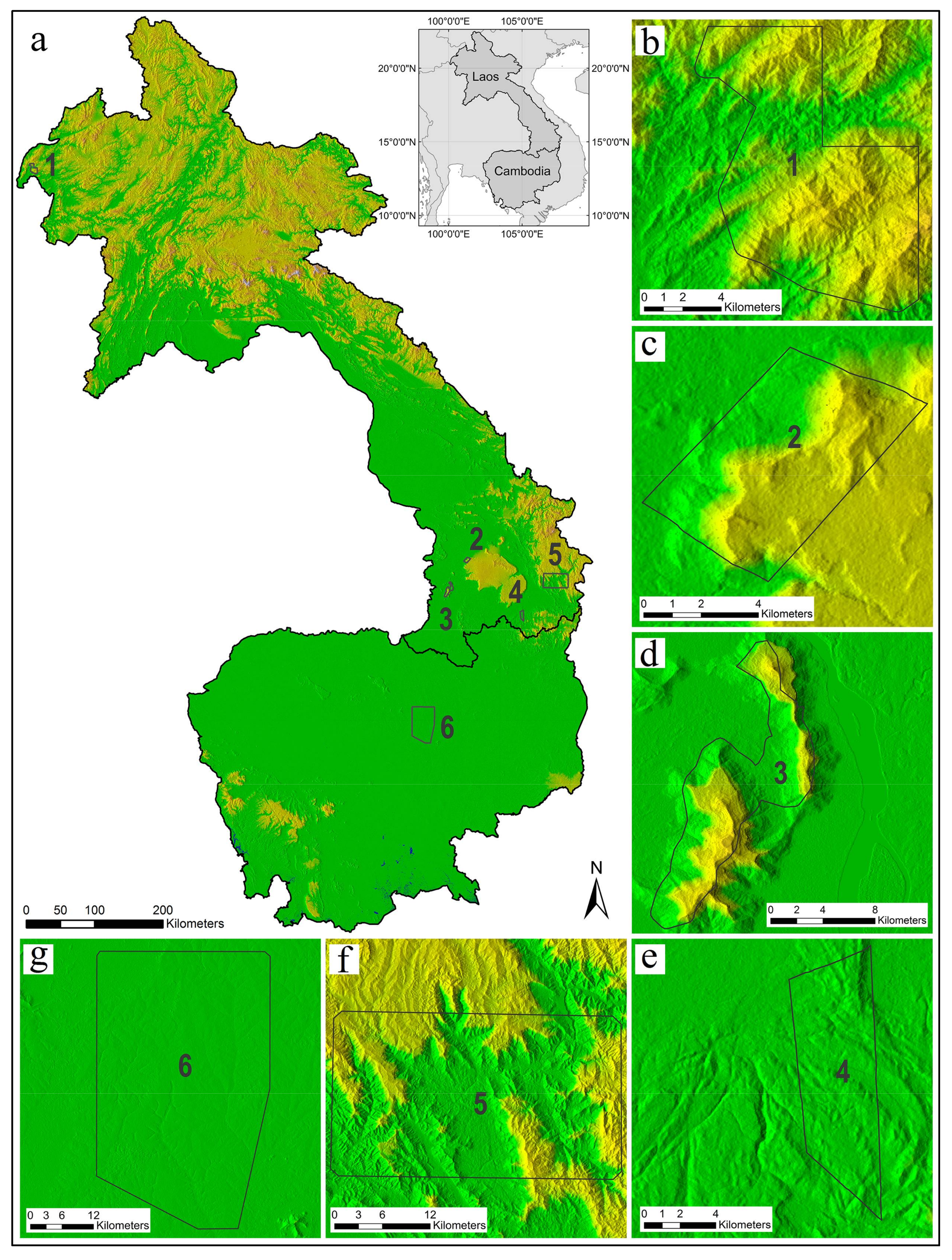
2.1. Study Area, Satellite and Auxiliary Data

In this study, we analyzed Landsat 8 imagery in order to detect crown cover disturbances within evergreen and semi-evergreen forests of Cambodia and Laos occurring in 2015 and 2016. Both countries are characterized by a tropical monsoon climate with a pronounced dry season from November to April [52]. The major inland forest and woodland types of the region belong to different ecosystems ranging from moist tropical rain forests to dry deciduous forests, with various intermediate types of semi-evergreen and semi-deciduous forests, and the typical dry Dipterocarp forests and woodlands. A clear separation between individual forest types by means of remote sensing is often difficult [53]. Over the last decades, these natural forest ecosystems have been under pressure by human intervention, including, for instance, large-scale conversions to cash crops and forest plantations, dam and road construction, as well as various types of logging [54].

We used all existing top-of-atmosphere (ToA) ortho-rectified Landsat 8 data (spatial resolution of 30 m) available in the GEE archive for the period from 1 January 2014 to 31 December 2016, covering the total area of Cambodia and Laos. This translates into a total number of 1030 and 1371 Landsat scenes for Cambodia and Laos, respectively. For the validation process, some additional Landsat 8 imagery stemming from 2013 and 2017 were processed to derive crown cover disturbance maps matching the acquisition dates of the very high resolution satellite images used as reference data (see Section 2.2.4).

For validation and accuracy assessment, we were restricted to defining six test sites determined by the availability of high (HR) and very high-resolution (VHR) satellite imagery over the target region (Figure 1a). Only for these sites, could we obtain pairs of reference satellite imagery, available at two points of time, as required for the validation of change (

Table 1. Test sites and VHR/HR imagery (type, acquisition date) used for validation.

Test Site	Country (Province)	Size in ha	Reference Scene 1	Acquisition Date 1	Reference Scene 2	Acquisition Date 2
1	Laos (Bokeo)	10,472	Pleiades	23 November 2015	Pleiades	7 February 2017
2	Laos (Champasak)	3979	Pleiades	31 January 2016	WorldView-2	19 February 2017
3	Laos (Champasak)	9672	Pleiades	25 January 2016/7 February 2016	Pleiades	22 January 2017/2 March 2017
4	Laos (Attapeu)	5517	WorldView-2	2 January 2015	GeoEye-1	14 February 2017
5	Laos (Attapeu)	75,157	RapidEye	14 February 2014	RapidEye	14 January 2015
6	Cambodia (Kampong Thom)	156,934	RapidEye	15 April 2014	RapidEye	30 March 2015

). A random selection of the test sites was therefore not possible. While the HR data (RapidEye, bands: 440–510 nm, 520–590 nm, 630–685 nm, 690–730 nm, 760–850 nm) have a spatial resolution of 5 m, all three VHR sensors (Pleiades, WorldView-2, GeoEye-1) are characterized by being resampled to a higher spatial resolution of 50 cm. However, these VHR sensors show differences in the characteristics of the spectral bands (Pleiades, bands: 430–550 nm, 490–610 nm, 600–720 nm, 750–950 nm; WorldView-2, bands: 400–450 nm, 585–625 nm, 705–745 nm, 860–1040 nm; GeoEye-1, bands: 450–510 nm, 510–580 nm, 655–690 nm, 780–920 nm), possibly influencing visual interpretation between different sensors. During the selection of the VHR data, off-nadir angles >20 degree were rejected to avoid unnecessary interpretation problems. However, VHR data for a total area of almost 30,000 ha, and additional HR data for more than 230,000 ha were obtained, covering forest areas typical for the region and having experienced various forest disturbance processes, such as shifting cultivation or selective logging. Furthermore, they differ in terms of the predominant topography. Whilst the test sites in Laos (Figure 1b–f) are characterized by more or less hilly and rugged terrain, the central Cambodia site (mostly belonging to the Prey Lang Wildlife Protected Area) has rather flat topography (Figure 1g).

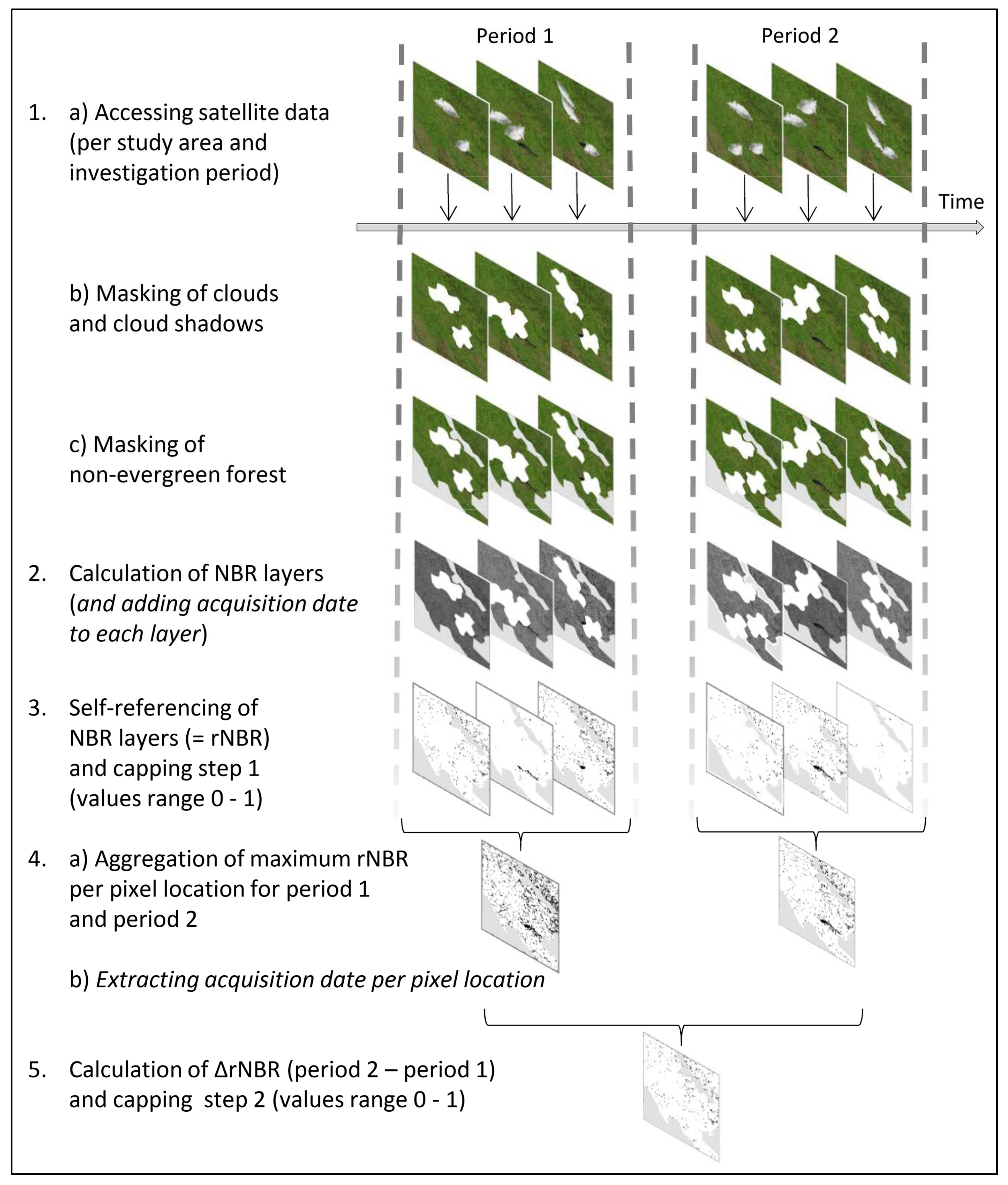
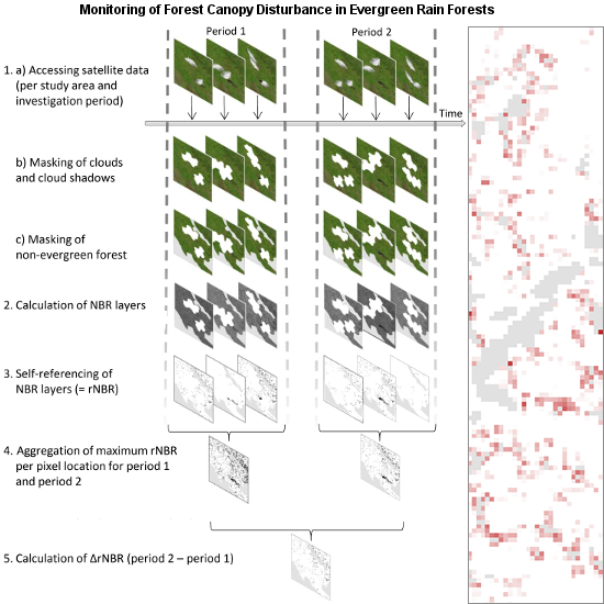
2.2. Methodology for Detecting Crown Cover Disturbance

This study focuses on tropical evergreen and semi-evergreen rain forests, hereafter referred to as ‘evergreen’ forests. For the detection of changes in canopy crown cover, indicating processes of forest disturbance or potential forest degradation, we calculated the difference (Δ) of a modified normalized burn ratio (rNBR) vegetation index, hereafter referred to as ‘ΔrNBR’, over consecutive periods. A GEE script was developed, aimed at operational processing and the analysis of large amounts of satellite data without any user interaction, but also performing the required steps of pre- and post-processing enabling inter-scene comparability and the temporal aggregation of the data. The processing chain can be broken down into five subsequent processing steps:

2.2.1. Masking of All Landsat ToA Scenes

All selected Landsat 8 data are masked automatically, selecting for further processing only those pixels identified as representing evergreen forest (‘evergreen forest maps’), and not affected by cloud or cloud shadow interference. We derived these evergreen forest maps from a pan-tropical forest dataset at 30 m spatial resolution, which displays evergreen forest cover as well as change to non-forest within an observation period and which is to be published soon (Vancutsem et al., personal communication). This dataset was generated by an automated classification (decision tree) of a time-series of 33 years of Landsat data (1984–2016), examining the photosynthetic activity (‘greenness’) for every pixel location and every single-date image. A pixel is classified as ‘undisturbed’ when always detected as fully vegetated over the 33-year period. The validation, presently only available for the African continent, shows an overall accuracy of 95.8% with 3.6% of omission and 4.3% of commission errors, respectively [55].

For our study, we derived from this dataset binary evergreen forest maps for the years 2014, 2015 and 2016, grouping the original classes ‘undisturbed forest’ and ‘old vegetation regrowth’ as ‘forest’ class (fully vegetated at least after 2006). Deforestation patches mapped with this approach can be as small as one Landsat pixel (0.09 ha). These maps display the forest status at the end of the respective year, and we use them to define evergreen forest pixels in all Landsat scenes acquired within that year.

To remove cloud- and cloud-shadow-affected pixels, we applied two different cloud-masking processes to each single Landsat scene. First, we detected clouds based on the Landsat 8 quality bands. Then, we used the ‘Fmask’ algorithm [56,57] to derive an additional quality band on cloud and cloud shadow detections. The combined result was amply buffered with 2500 m (corresponding to 84 Landsat pixels at 30 m spatial resolution) to remove possible cloud edges or cloud remnants that had not been masked properly. The application of strict cloud removal procedures was crucial in this study, as the remaining clouds may lead to false positive detections of crown cover openings (errors of commission) within the single scenes. Eventually, the boundary of each Landsat scene was buffered by 500 m (corresponding to 17 Landsat pixels) inwards in order to cut off scene edges, which can be affected by sensor artifacts.

2.2.2. Calculation of NBR for Each Scene

We then calculated the NBR (Equation (1)) for each single masked Landsat 8 scene with NIR referring to Landsat 8 band 5 (0.85–0.88 µm) and SWIR₂ to band 7 (2.11–2.29 µm).

$$NBR=\frac{NIR-SWI{R}_2}{NIR+SWI{R}_2}$$

(1)

The results were floating point values ranging between −1 and 1. Within the evergreen forest maps, larger NBR values generally refer to a closed crown cover, whilst smaller values reflect openings in the canopy, exposing components of bare soil or non-photosynthetic vegetation, for example caused by the removal of single trees. Forest disturbance can even be at the sub-pixel scale—crucial is only the exposure of these components that can be detected by the NBR index. However, especially in the humid tropics, the appearance of these components is ephemeral due to a fast growing layer of ground cover/saplings. This temporal aspect was taken into account using all available Landsat 8 imagery for a period in order to ensure the shortest possible time lag between the disturbance event and satellite acquisition.

2.2.3. Self-Referencing of Masked NBR Scenes

It is important to note that the attributes ‘larger’ and ‘smaller’ used above are relative terms, i.e., two scenes of unequal atmospheric conditions or illumination geometries will generally result in different NBR values [50], thus restraining direct comparison of the values stemming from different scenes. We therefore introduced a step of self-referencing, removing such differences and enabling comparability between different scenes.

While atmospheric or illumination effects cause gradual changes in the NBR signal over large portions of a single scene, human disturbances—such as the construction of logging roads, selective logging or shifting cultivation activities—result in locally abrupt, small-scale differences in the signal [58]. To focus on small-scale changes only, we used a circular moving kernel window, calculating the median over the direct neighborhood of each pixel location for the above-derived NBR results, and then subtracting the actual NBR pixel value from the median value (Equation (2)). This approach removes gradual changes, but retains any abrupt alteration of NBR values. Thus, while self-referenced NBR values (rNBR) of undisturbed canopy cover display values close to 0, the rNBR of canopy cover openings shows positive values. The choice of a circular kernel stems from its ability to weight any kind of pixel pattern equally [59]. This self-referencing process is performed for every single NBR result.

$$rNBR=NB{R}_{n_{median}}-NBR$$

(2)

The size of the moving kernel radius (n in Equation (2), in meters) is chosen as a compromise to remove atmospheric or illumination/terrain-related effects and at the same time to conserve small-scale changes in the canopy crown cover condition. The characteristic feature of this self-referencing process is its focus on the reliable detection of only small-scale crown cover disturbances within otherwise closed evergreen tree cover. The term ‘small-scale’ refers here to canopy openings covering less than half of the applied kernel size. The smaller the kernel window (e.g., 30–60 m radius, or one to two Landsat pixels), the more precise unwanted effects can be corrected. This is especially important when dealing with intermediate-scale effects caused by illumination within mountainous areas of steep topography.

However, the trade-off of this self-referencing step is the detection of abrupt changes covering more than half of the kernel size. In this case, the applied approach results in artifacts of alternating larger and smaller rNBR values even though homogeneous larger rNBR values are to be expected. This stresses the importance of the quality of the above-derived evergreen forest maps. In our study, a 210 m radius kernel (7 Landsat pixels) was applied, providing a good compromise between the ability to remove unwanted effects and the avoidance of artifacts.

While openings in the canopy cover result in positive rNBR values during the self-referencing step, patches of pixels with very dense vegetation cover can show slightly negative values. As our monitoring approach aims to detect crown cover openings within otherwise undisturbed canopy cover (rNBR values very close to 0), we neglected any negative values by setting them to 0, avoiding unwanted offset when calculating the difference between two periods (see Section 2.2.5). In addition, values above 1 were capped because these extreme values usually refer to active fires and strongly exceed the pixel values of bare soil or non-photosynthetic vegetation. The percentage of pixel values >1 was, however, negligible with 0.002‰ and 0.003‰ over the whole investigation periods for the complete countries of Cambodia and Laos, respectively (aggregated over all processed Landsat scenes). The capping conditions are finally reflected in Equation (3).

$$rNB{R}_{cap}=\{\begin{array}{c}1forrNBR>1\\ rNBRfor0\le rNBR\le 1\\ 0forrNBR<0\end{array}$$

(3)

2.2.4. Temporal Aggregation of Data

The chances of detecting a canopy cover opening using the rNBR are higher shortly after the disturbance event (see Section 2.2.2), because in the tropics a fast growing ground cover/saplings layer can quickly cover any exposed bare soil or non-photosynthetic vegetation, which has a crucial impact on the detection process. Thus, the shorter the time lag between a disturbance event and subsequent satellite acquisition, the more accurate the detection of that event. For this reason, our approach analyzes all available pre-processed Landsat 8 scenes, finally condensing the data to canopy closure maps by memorizing only the maximum rNBR_cap value (referring to the largest crown cover opening) found for each pixel location within a certain temporal window (Equation (4)). Furthermore, as single scenes may—at least in parts—be obscured by cloud cover, the use of all available Landsat 8 scenes significantly enhances the chance of deriving wall-to-wall information.

$$rNB{R}_{cap\_max\_y}=\underset{01.01.y\le i\le 31.12.y}{\max }(rNB{R}_{cap\_i})fory\left(y=2014,\dots ,2016\right)$$

(4)

Thus, the canopy closure maps for three individual years (2014–2016), each depicting the most open crown cover condition within that year, were finally used to generate countrywide ΔrNBR maps (see Section 2.2.5). Furthermore, the Landsat acquisition dates of the corresponding maximum rNBR_cap values were stored in a supplementary time-stamp file, providing additional information on the timing of the disturbance events.

For consistent validation, we produced separate ΔrNBR maps for the six test sites, using only Landsat 8 scenes from the period most closely matching the acquisition dates of the corresponding VHR/HR reference image pairs. Temporal aggregation is done according Equation (4), adjusting, however, the start and end date of each period and site to match the reference period (

Table 2. Overview of the start and end dates of the two Landsat 8 acquisition periods for the validation exercise. The last column shows the number of Landsat 8 scenes involved to derive the ΔrNBR per test site.

Test Site	Country (Province)	Landsat Start Period 1	Landsat End Period 1	Landsat Start Period 2	Landsat End Period 2	Number Scenes
1	Laos (Bokeo)	24 November 2014	23 November 2015	24 November 2015	5 March 2017	46
2	Laos (Champasak)	1 February 2015	31 January 2016	1 February 2016	5 February 2017	43
3	Laos (Champasak)	26 January 2015	25 January 2016	26 January 2016	5 February 2017	81
4	Laos (Attapeu)	3 January 2014	2 January 2015	3 January 2015	14 February 2017	61
5	Laos (Attapeu)	11 April 2013	14 February 2014	15 February 2014	25 January 2015	65
6	Cambodia (Kampong Thom)	16 April 2013	15 April 2014	16 April 2014	21 April 2015	39

). Thus, period 2 does not necessarily correspond to a regular 12 months, and if covering more than one turn of the year (as for study sites 1 and 4), only the latest forest map was used. In order to finally calculate the ΔrNBR, an additional period of 12 months preceding the first acquisition (period 1 in Table 2) date was used where feasible, taking into account that Landsat 8 fully entered service only on 11 April 2013. Considering further the 16 day overpass cycle of Landsat 8 and the difficulty in obtaining cloud-free imagery, the last acquisition dates for period 2 (period 2 in Table 2) were—whenever possible—slightly shifted to a subsequent cloud-free date to best fit the acquisition dates of the reference scenes.

As temporal mosaics of reference imagery were used for both acquisition times for test site 3 (Table 1), the corresponding Landsat 8 data were aggregated over a corresponding period from January 2016 until March 2017 for that site.

2.2.5. Calculation of ΔrNBR

Lastly, in order to separate actual disturbance events within evergreen forests from permanent canopy openings (e.g., limestone pinnacles within an otherwise closed tree cover), it was necessary to compare crown cover conditions from different periods and to map only the changes. This was done by calculating the difference between the rNBR_{cap_max_y} results from the years 2014 until 2016, as derived under Section 2.2.4 (Equation (5)).

$$\Delta rNB{R}_{y+1}=rNB{R}_{cap\_max\_y+1}-rNB{R}_{cap\_\max \_y}fory\left(y=2014,2015\right)$$

(5)

Thus, the ΔrNBR for 2015 and the ΔrNBR for 2016 were derived, showing the difference between the canopy closure maps for two subsequent calendar years each (e.g., the canopy closure of 2015 was compared to the canopy closure of 2014, resulting in the ΔrNBR of 2015 map). Similarly, for validation, the ΔrNBR products of the six study sites were calculated using the periods given in Table 2.

The combination of the sensitivity of the rNBR index to soil or non-photosynthetic vegetation and the short-lived nature of these signals lead to ΔrNBR results showing both negative and positive values. It is important to realize that while positive values refer to openings in the canopy cover (e.g., by the removal of single trees), negative values may show re-greening, but usually do not reflect a closure of the canopy cover by the regrowth of tall trees, given the short time span of maximum two years. This ‘re-greening’ rather shows the disappearance of the detectable soil or non-photosynthetic vegetation component due to the growth of ground-covering plants and saplings of short-lived pioneer tree species. Therefore, a second capping step is introduced, resetting all negative ΔrNBR values to 0 (Equation (6)).

$$\Delta rNB{R}_{y+1\_cap}=\{\begin{array}{c}\Delta rNB{R}_{y+1}for\Delta rNB{R}_{y+1}\ge 0andy\left(y=2014,2015\right)\\ 0for\Delta rNB{R}_{y+1}<0andy\left(y=2014,2015\right)\end{array}$$

(6)

Ultimately, the final countrywide ΔrNBR_{y+1_cap} products and the temporally adjusted ΔrNBR_{y+1_cap} products for the six validation sites as well as the corresponding time stamp datasets of each of the rNBR_{cap_max_y} intermediate results were exported and downloaded from GEE. Figure 2 provides a flow chart of all major processing steps.

2.3. Validation and Accuracy Assessment

For validation, we looked at three different components: (i) field-survey to obtain an understanding of local causes and the appearance of the canopy disturbance; (ii) the actual accuracy assessment based on VHR (50 cm) satellite imagery; and (iii) a comparison between accuracy figures obtained over flat and mountainous terrain using HR (5 m) satellite imagery.

2.3.1. Field Survey

Field surveys were undertaken in Laos (Salavan and Champasak provinces) and in Cambodia (Kampong Thom province) in February and March 2017, visiting 73 and 107 forest locations, respectively. The main objective of the fieldwork was to obtain a good understanding of the performance of the ΔrNBR approach in relation to field observation. The plots were selected to meet the following criteria: (i) the corresponding pixels display (even minor) ΔrNBR signals in 2015 or 2016; (ii) accessible with reasonable effort; and (iii) the required official permission to enter the respective forests could be obtained from the province administration. However, due to non-randomness, the field observations were not used for the quantitative accuracy assessment.

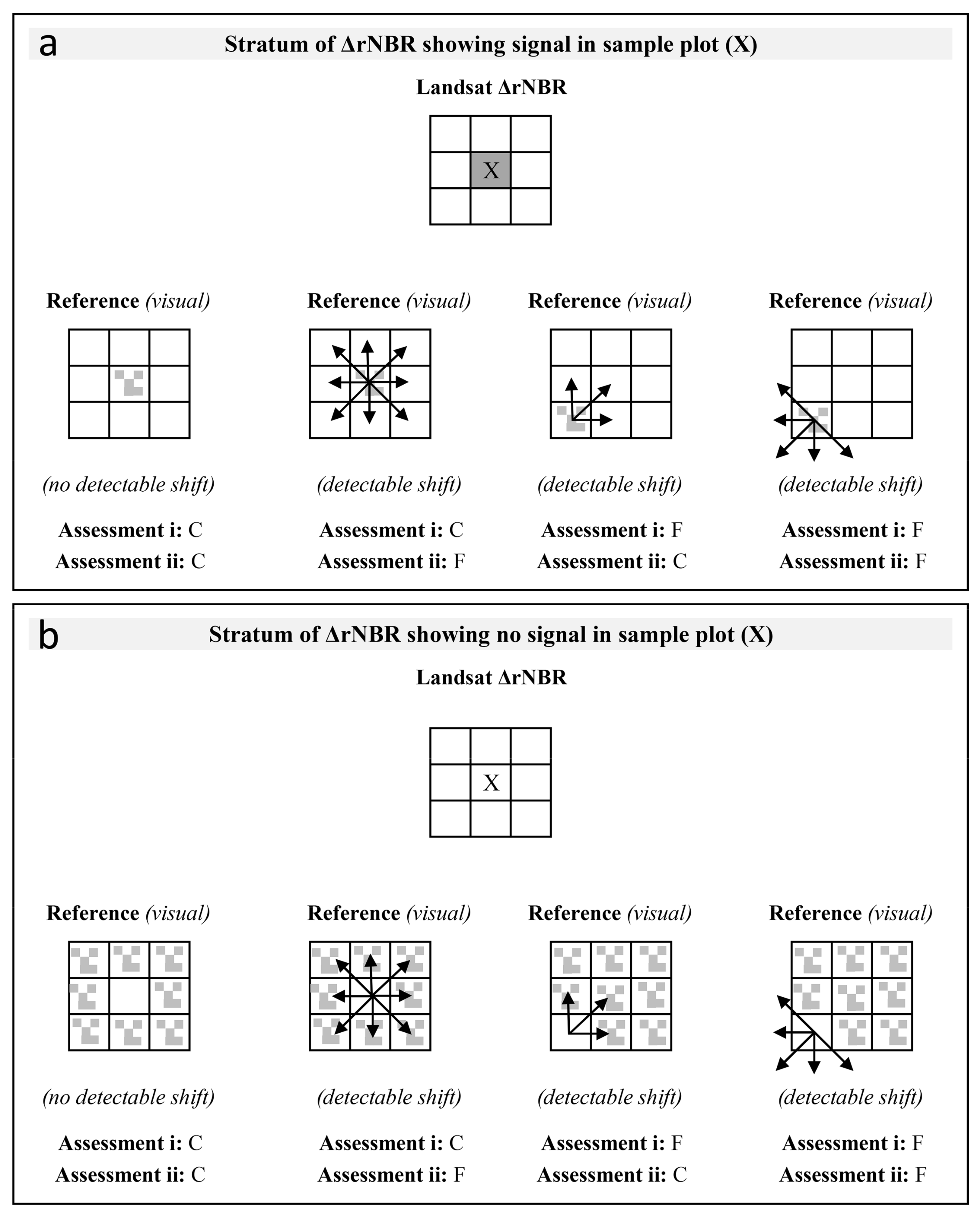
2.3.2. Accuracy Assessment Based on VHR Reference Satellite Imagery

In order to identify small-scale openings in the canopy cover, as expected to be detected by the ΔrNBR, reference datasets of higher spatial resolution are mandatory for validation. In addition, as the ΔrNBR signals refer to canopy closure change, two reference scenes from the end of both investigation periods are required. Furthermore, instead of comparing the canopy closure conditions at two points in time, the ΔrNBR approach works with temporal composites of two investigation periods that reflect the most open canopy closure condition per pixel location occurring within each investigation period. We assume that the crown cover disturbance occurring within an investigation period can still be identified on the reference image acquired at the end of that period. We calculate specific ΔrNBR results for the four VHR test sites 1–4, exactly matching the periods covered by the particular reference image pairs. The reference scenes have a spatial resolution of 50 cm (GeoEye-1, Pleiades, WorldView-2; Table 1) and the investigation periods of the corresponding Landsat scenes are given in Table 2. Minimal shifts between the acquisition times of the reference scenes and those of the corresponding Landsat data have to be tolerated (see Section 2.2.4).

For validation, we stratified the pixels of the ΔrNBR datasets for the test sites into two strata, namely ‘crown cover disturbance’ and ‘no disturbance, including noise’, using a threshold of 0.02, empirically-derived and supported by field observation. We then randomly selected 50 points per stratum within each of the test sites. Finally, all 400 points were visually checked with the reference datasets, allowing the calculation for each test site of the overall accuracy as well as user and producer accuracies after applying weighting factors [60,61], reflecting the different portions and therefore the difference in sampling probability for disturbed and un-disturbed pixels.

Furthermore, we derived F1 score values [62] as a harmonic mean between user and producer accuracy, which conservatively describe the results, derived from unbalanced user and producer accuracies. Additional information from the time stamp datasets showing the acquisition dates per single rNBR period helped us to understand the temporal context of the ΔrNBR value per sample point.

As the reference scenes show distortions up to 15 m among themselves as well as compared to the Landsat data, a ‘rigid’ (type i) and a more ‘flexible’ (type ii) assessment approach were applied in parallel (Figure 3). For the ‘rigid’ assessment (type i) we strictly focused on the extent of the Landsat pixel (marked with an X in Figure 3) selected by each random sample point and checked it against the corresponding area in the reference scenes, neglecting any shift between the different scenes and thus providing a ‘worst-case scenario’. For the ‘flexible’ assessment (type ii) we analyzed a 3 × 3 Landsat pixel window around each sampling point, which permitted us to account for possible distortions between the datasets, thereby allowing a possible shift of maximum one Landsat pixel and accepting bearing deviations of up to ±45 degree if the pattern was confirmed by the reference scenes. Finally, a total of 400 reference points were visually interpreted two times, using ArcGIS. Eventually, confusion matrices were calculated between the ΔrNBR values and the visually-derived results. In contrast to assessment type i, type ii is not blinded, as the interpreter has to have information about the ΔrNBR signal for the actual pixel location as well as its vicinity.

2.3.3. Analysis of the Possible Effects of Topography

Similar to the VHR sites, specific ΔrNBR results for the two HR test sites 5–6 (based on 5 m RapidEye reference data; Table 1 and Table 2) were calculated to match the periods covered by the reference image pairs. In comparison to the VHR reference data, the HR data had a lower spatial resolution that restricted the visual identification of changes in forest canopy closure. To account for the latter, we raised the threshold for discriminating between signal (crown cover disturbance) and noise (no crown cover disturbance) from 0.02 to 0.03. As both test sites were considerably larger than the VHR sites, the number of sample points per stratum was set to 100, which were weighted to account for the unbalanced strata populations. Similar to the VHR sites, a total of 400 reference points were visually interpreted two times. Overall accuracies and F1 score values of both sites were compared with each other to obtain an indication of whether the ΔrNBR was compromised by topographic effects.

3. Results

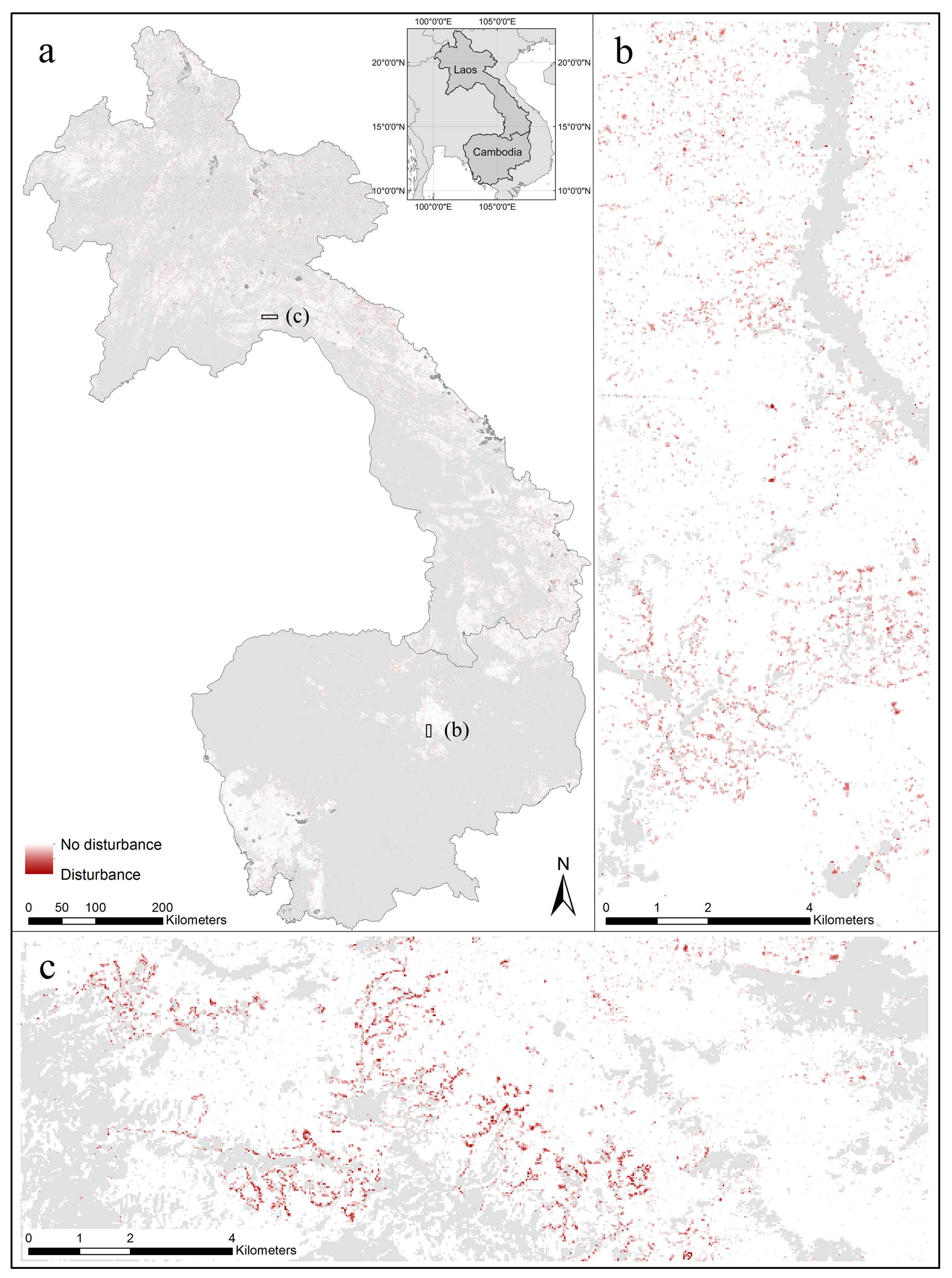
3.1. Country-Scale ΔrNBR Disturbance Maps

The ΔrNBR results display seamless countrywide wall-to-wall maps of forest canopy disturbance over Cambodia and Laos (Figure 4a–c). There are no obvious artifacts, despite the compositing and mosaicking of data stemming from multi-temporal scenes with different sun incidence angles and varying atmospheric conditions. Small-scale forest canopy disturbances—even those occurring at sub-pixel level, as for example by the extraction of individual trees—are reflected by ΔrNBR values at the level of single or few adjacent pixels. Linear patterns typically stemmed from logging roads and access trails.

Agglomerations of pixels with relatively large ΔrNBR values often indicate the initial phase of shifting cultivation and may be regarded as small-scale deforestation patches. Pixels with disturbance signals encircling already-existing (small) non-forest patches point at further encroachments into the surrounding forests. Particularly diffuse patterns of individual pixels do not always point towards anthropogenic disturbance, but may also be caused by individual living defoliated trees, naturally dead trees, dried or dead stands of bamboo or dead lianas covering other vegetation. Within the 2016 ΔrNBR map for Laos, pixel patches fringing non-forest areas along higher mountain ridges above 1000 m represent a vegetation dieback due to fires following a combination of the 2015–2016 El Niño event and an extremely cold spell with freezing rain in the dry season 2015–2016 (personal communication, S. Koch, GIZ Laos).

3.2. Analysis of Field Plot Data

The evaluation of 180 field plots in Cambodia and Laos suggested a ΔrNBR threshold of 0.01 as a first approximation to separate in the field possible disturbance signals from noise. For field analysis, even ΔrNBR values caused by minor changes in canopy closure, detectable from the ground—e.g., dead lianas partially covering other vegetation, broken larger branches with dried leaves, defoliated but maybe still living trees—are considered as correctly detected ‘disturbance’ events. Assessed in such a way, the ΔrNBR values over all ground plots in Cambodia and Laos resulted in correct indications of canopy disturbance in 97.1% and 94.5% of the cases, respectively. However, it has to be noted that such minor disturbances do not constitute actual forest degradation and the incorporation of such events is likely to lead to exaggerated statistics. In addition, as the sample of field plots is based only on pixels where the ΔrNBR shows some signal (ΔrNBR > 0), the sampling is not probabilistic and therefore, the above values do not represent any accuracy assessment.

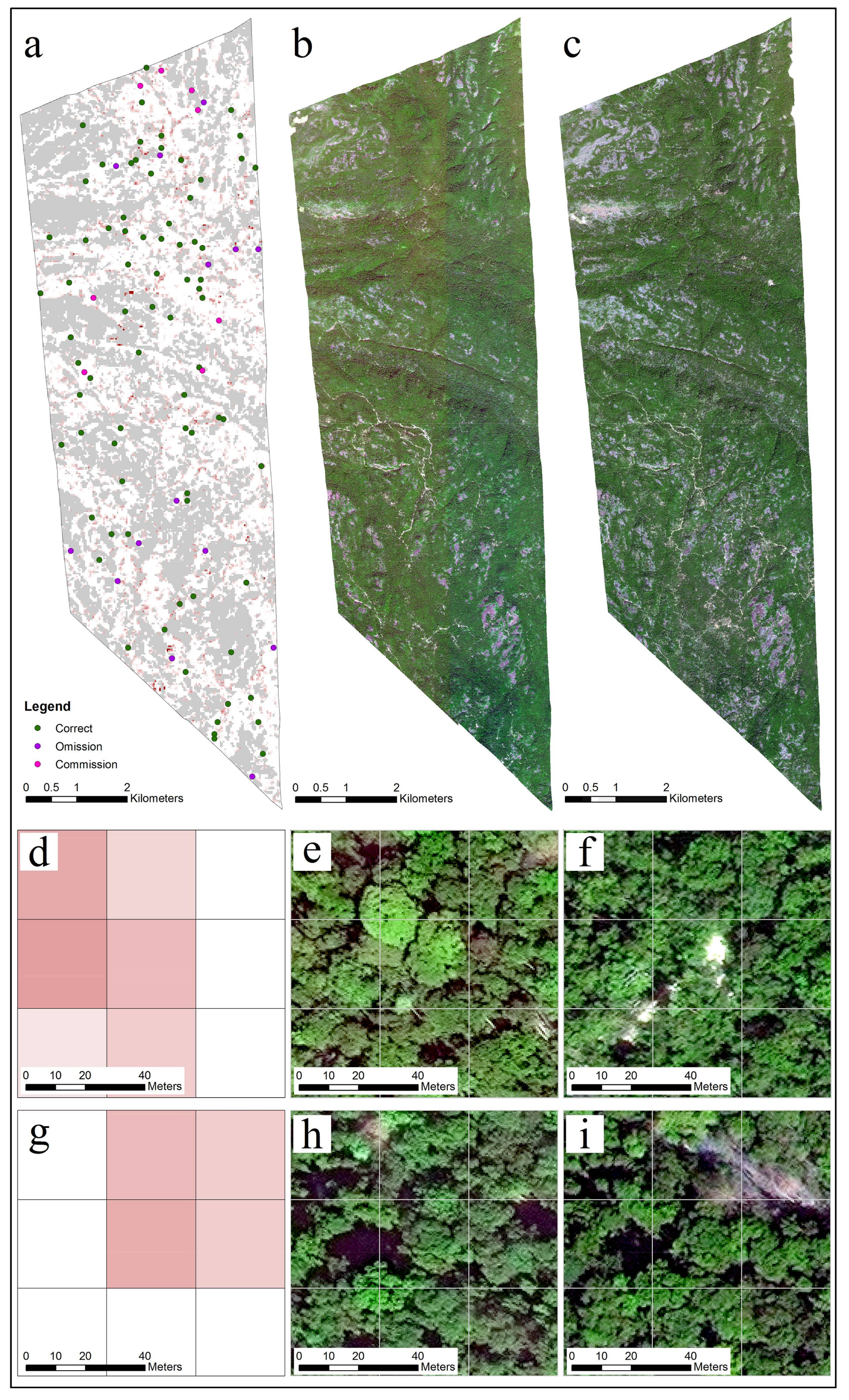
3.3. Accuracy Assessment Based on VHR Reference Imagery

The overall accuracies for all four VHR test sites were assessed at 73.2% (F1 score: 0.54701) and 77.7% (F1 score: 0.61452) for type i and type ii assessments, respectively.

Table 3. Results of accuracy assessments of the ΔrNBR products (0.02 threshold) derived for the four VHR study sites; (i) refers to the results of accuracy assessment type i; (ii) refers to assessment type ii; D = disturbance stratum; N = no disturbance stratum; SPS = stratum population size; F1 = F1 score; OA = overall accuracy; PA = producer accuracy; UA = user accuracy.

Site	SPS		F1	OA	PA	UA
	Assessment over all four VHR sites
1–4 (i)	D	4404 ha	0.54701	73.2%	45.8%	67.8%
	N	14,084 ha			88.2%	74.9%
1–4 (ii)	D	4404 ha	0.61452	77.7%	52.2%	74.6%
	N	14,084 ha			90.8%	78.7%
	Assessment per single VHR site
1 (i)	D	1062 ha	0.45375	70.9%	34.6%	66.0%
	N	4736 ha			90.4%	72.0%
1 (ii)	D	1062 ha	0.50513	72.7%	37.8%	76.0%
	N	4736 ha			93.0%	72.0%
2 (i)	D	660 ha	0.57300	69.7%	46.7%	74.0%
	N	1737 ha			87.3%	68.0%
2 (ii)	D	660 ha	0.69016	78.8%	57.6%	86.0%
	N	1737 ha			93.5%	76.0%
3 (i)	D	1712 ha	0.58241	78.7%	54.9%	62.0%
	N	5446 ha			87.6%	84.0%
3 (ii)	D	1712 ha	0.63309	82.3%	62.6%	64.0%
	N	5446 ha			88.6%	88.0%
4 (i)	D	971 ha	0.59311	67.7%	48.6%	76.0%
	N	2165 ha			85.6%	64.0%
4 (ii)	D	971 ha	0.68172	75.7%	57.4%	84.0%
	N	2165 ha			90.9%	72.0%

provides an overview of overall accuracies, F1 score values, and producer and user accuracies for each of the four sites. The choice of a slightly more conservative ΔrNBR threshold for the accuracy assessment—i.e., including only ΔrNBR values larger than 0.02—can be attributed to the fact that very small-scale disturbance events, which mostly do not constitute actual forest degradation, were detectable in the field, but not consistently on the VHR reference imagery. Figure 5 shows the sampling design of a showcase including the assessments of each sampling point.

3.4. Effects of Topography

Using a threshold of 0.03 for the comparison of the results obtained for the HR sites of rugged and flat terrain (sites 5 and 6), the overall accuracies and F1 scores (

Table 4. Accuracy values of the ΔrNBR products (0.03 threshold) derived for the two HR study sites to analyze topographic effects; (i) refers to accuracy assessment type i; (ii) refers to assessment type ii; D = disturbance stratum; N = no disturbance stratum; SPS = stratum population size; F1 = F1 score; OA = overall accuracy; PA = producer accuracy; UA = user accuracy.

Site	SPS		F1	OA	PA	UA
5 (i)	D	4186 ha	0.43807	86.8%	31.7%	71.0%
	N	53,425 ha			97.5%	88.0%
5 (ii)	D	4186 ha	0.49067	88.8%	36.7%	74.0%
	N	53,425 ha			97.8%	90.0%
6 (i)	D	4709 ha	0.31675	85.0%	19.5%	84.0%
	N	108,744 ha			99.2%	85.0%
6 (ii)	D	4709 ha	0.38189	88.0%	24.3%	89.0%
	N	108,744 ha			99.5%	88.0%

) suggest that the ΔrNBR approach can cope well with different topographies. Indeed, both assessment types i and ii show even larger values for rugged terrain (overall accuracies: 86.8% and 88.8%, respectively) than for flat topography (overall accuracies: 85.0% and 88.0%, respectively).

4. Discussion

4.1. Main Characteristics of the Proposed Approach

The ΔrNBR approach presented in this study allows the processing and compositing of large numbers of satellite scenes and the production of seamless wall-to-wall ‘disturbance’ maps at national or regional scales. This is accomplished to a large extent by introducing a step of ‘self-referencing’ for each single-date NBR product. The process is essential to correcting for illumination artifacts over topographically heterogeneous landscapes and to rectify the influence of varying haze or other atmospheric conditions. Whilst for undisturbed forest canopies the rNBR shows values close to 0, the relative magnitude of any abrupt change, as caused by canopy disturbances, is kept in the signal. This offers two advantages: Firstly, it enables inter-scene comparability, allowing the processing and compositing of large numbers of satellite scenes into seamless wall-to-wall maps, reflecting for each pixel location the most open crown cover condition found within each investigation period. Secondly, even slight changes in canopy cover between the investigation periods can be detected.

Furthermore, during the implementation of the ΔrNBR methodology there is no requirement for any user interaction. The output is therefore transparent and reproducible, increasing the credibility and applicability for monitoring, reporting and verification (MRV), as for example required for REDD+. Approaches like SMA, for instance, require the definition of pure spectral endmembers [26,28]. The quality and consistency of the output can therefore vary depending on the user input. In addition, radiometric normalization based on pseudo-invariant features may be required [32,63].

A further essential feature of the ΔrNBR approach is the exploration of the full revisiting capability of satellite image acquisition for a desired period, retaining a disturbance signal even if detected only once through the observation period. This is a prerequisite for coping with often short-lived disturbance signals in tropical conditions and for not missing disturbance events. For example, field visits in Laos and Cambodia reveal that the two main components of the ΔrNBR detected canopy disturbance stem either from the sawn wood and tree crowns remaining in the forest as non-photosynthetic vegetation or from exposed soil. Due to the tropical climate, a fast growing layer of ground-covering plants, together with saplings of short-lived pioneer tree species, can quickly overgrow and hide these detectable components, underlining the importance of using a possibly large number of satellite image acquisitions over the investigation period.

Finally, focusing directly on the aspect of ‘change’ is seen as advantage for reporting on ‘activity data’ in the context of REDD+. It also prevents areas of permanently open canopy cover (e.g., specific soil conditions, natural outcrops) or previous forest conversion sites to be erroneously included as forest disturbance.

4.2. Post-Processing Threshold Setting

The setting of a threshold for the derived ΔrNBR result can be a useful step to exclude potential noise. It is only at this post-processing stage that the user can modify the original ΔrNBR output by excluding a certain range of (low) ΔrNBR values. The treshold setting can be supported by testing its impact on excluding single pixels diffusely distributed over the target area, which may represent noise. For reasons of consistency, a once-selected threshold value needs to be maintained.

4.3. Challenges and Limitations

Single leave-shedding trees, dried bamboo or mixed forest stands of notable deciduous phenology—although included in the evergreen forest maps—can cause commission errors. The monitoring of forest degradation events within forests of varying levels of seasonality is challenging in general [16]. Indeed, the larger portion of deciduous trees within study site 1 may have led to the lower F1 scores compared to the other study sites, because the spectral signal—stemming from temporary seasonal effects—may already have vanished at the acquisition time of the second VHR scene. Particularly in very dry years, seasonal components in semi-deciduous forests may wrongly be interpreted as disturbance events. This is also true when lianas, covering other vegetation, experience sudden dieback. In such extreme cases, even the analysis with VHR reference data does not allow the reliable separation of the above-described commission errors from ‘real’ forest disturbance events.

Clouds not detected and masked during pre-processing can result both in errors of omission and commission. For example, undetected clouds in period 2 may have resulted in commission errors as wrongly considered ‘canopy openings’. However, undetected clouds in period 1 may have caused omission errors only in the case of actual canopy change at the same location in period 2. Even though the applied automated cloud-masking processes perform very well, the removal of still undetected clouds due to invasive cloud buffering further considerably improves this pre-processing step.

The correlation between the ΔrNBR values and the intensity of the disturbance events is influenced not only by number or by size of trees extracted but also by the amount of exposed soil or non-photosynthetic vegetation being detected. However, the latter may vary depending on factors, such as neighboring large tree crowns still covering the soil, the way the logged trees are further processed, the acquisition date of the second image in relation to the actual disturbance event, or the existence of previous disturbance at sub-pixel level. Thus, differentiation into several disturbance classes according to the magnitude of the ΔrNBR signal is not considered in this study.

Furthermore, the same logged tree may result in signals in two different periods, if on-site processing and extraction (affecting vegetation regrowth) is applied to more than one observation period after felling.

Finally, the use of a moving kernel, which allows inter-scene comparability, can cause artificial patterns of undulating signals in cases where disturbed areas cover more than half of the circular kernel window. This can be avoided by increasing the kernel size, though limiting the ability to correct for smaller-scale illumination artifacts along mountain ridges and slowing down the processing time. Empirical analysis in our study indicates a kernel radius of 210 m as a good compromise between the avoidance of the different types of artifacts and processing time, detecting at the same time any kind of logging gaps. However, the use of high accuracy evergreen forest maps temporally fitted to the ΔrNBR results, minimizes possible artifacts by already excluding larger areas of ‘disturbance’ as ‘non-forest’ on these maps.

4.4. Accuracy Assessment and Performance

The overall accuracy values derived for the four VHR test sites point towards the satisfying performance of the ΔrNBR approach in reliably monitoring forest disturbance within evergreen forests. The VHR reference data further confirm that even Landsat sub-pixel-scale disturbance events as small as 0.005 ha can be detected, which are almost undetectable to a human interpreter of Landsat imagery, even when applying intense histogram stretching.

However, drawing direct conclusions for the country products based on the test site results is hampered for two reasons: First, the test sites could not be selected randomly, but depend in terms of number and spatial distribution on the availability of VHR reference imagery. A possible adjustment approach for reducing potential bias caused by the non-probabilistic sampling scheme [64] was not applicable to our study. Second, whilst the ΔrNBR products generated for the accuracy assessment temporally match the acquisition dates of the four VHR test sites, they differed in that respect from the generated ΔrNBR country products. However, such limitations constitute common ‘working conditions’ for remote sensing applications over tropical rain forests. Considering that almost 30,000 ha are covered with VHR reference imagery, one may take the findings of the accuracy assessment as the best possible approximation for validating the presented monitoring approach.

The analysis of the ΔrNBR approach over flat and rugged terrain based on HR (5 m) data displayed comparable results for the two test sites, suggesting therefore the overall robustness of the methodology against the effects of atmosphere and terrain. However, a direct comparison to the results obtained in the above accuracy assessment cannot be made, because due to the different type of reference imagery and the different ΔrNBR thresholds applied, the latter reflecting the reduced potential of HR imagery in visually identifying canopy cover disturbances. Due to their lower spatial resolution, different sensor incidence angles and acquisition times can result in possible geometric and illumination artifacts, leading to misinterpretations of the actual situation on the ground—particularly in cases of minor canopy disturbances.

4.5. Outlook

For operational use, a further refinement of the ΔrNBR may be considered by applying spatial filtering to single isolated pixels (implemented as an option in the freely available GEE script). A diffuse and homogenous distribution of single pixels across forest surfaces, not displaying any spatial pattern that can be related to any driver of disturbance, may be taken as an indication of these pixels representing noise rather than actual canopy disturbance. This step, however, requires an assessment based on regional knowledge. In such case, the reliability of the final product indicating disturbances and potential forest degradation may be further increased.

Furthermore, until now, the operational use of the ΔrNBR approach with Sentinel-2 (S2) data was not feasible due to insufficient data availability. First testing of single day S2 data has shown promising results [50]. Moreover, with revisiting times of five days and 10 m spatial resolution, we expect an increased potential for the operational real-time monitoring of forest canopy disturbances and related forest degradation processes.

5. Conclusions

In this study, we present a forest canopy disturbance monitoring methodology (called the ΔrNBR approach) based on medium-resolution satellite imagery that allows the detection of disturbance events at the sub-pixel level with satisfying accuracy. A ‘self-referencing’ procedure enables inter-scene comparability by removing atmospheric/topographic artifacts, thus allowing the processing of large numbers of satellite scenes and deriving seamless wall-to-wall forest disturbance maps at national or regional scales. The monitoring approach, implemented as a Google Earth Engine script, requires almost no user-interaction, thus providing consistent results. The access to extensive time series of satellite imagery with short repetition rates, such as Landsat or Sentinel 2, as provided by the Google Earth Engine archives is important. The script allows the analysis of any desired (also historic) period as long as sufficient imagery is available. Using Google cloud computing, the script can quickly process a full series of satellite images over a defined observation period, thus retaining canopy disturbances even if only detected once. This is essential for tracing forest degradation processes in the tropics, as canopy disturbances can become quickly invisible due to fast re-growing vegetation. A clear advantage of our monitoring approach lies in its capacity to deal with large amounts of satellite imagery in an automated way, where any visual interpretation would probably already fail in the initial phase, while only screening such a number of images. Due to its transparent methodology, this automatic monitoring approach will be of interest for MRV (monitoring, reporting and verification) in the context of REDD+ (reducing emissions from deforestation and forest degradation) or under FLEGT (forest law enforcement, governance and trade) for identifying logging activities. Integrating Sentinel 2 data will further increase the potential for operational real-time monitoring of forest degradation processes.

For development versions of the ΔrNBR script (Google Earth Engine account necessary) please see https://github.com/Andi1974/Forest-degradation-monitoring. For the latest archived version of the library, use DOI https://doi.org/10.5281/zenodo.1014728. Already processed ΔrNBR maps covering several Southeast Asian countries (further areas from other continents will be added) can be accessed at http://forobs.jrc.ec.europa.eu/recaredd/.

References

1. Achard, F.; Beuchle, R.; Mayaux, P.; Stibig, H.-J.; Bodart, C.; Brink, A.; Carboni, S.; Desclée, B.; Donnay, F.; Eva, H.D.; et al. Determination of tropical deforestation rates and related carbon losses from 1990 to 2010. Glob. Chang. Biol. 2014, 20, 2540–2554. [Google Scholar] [CrossRef] [PubMed]
2. FAO. Global Forest Resources Assessment 2010; FAO: Rome, Italy, 2010; p. 350. ISBN 978-92-5-106654-6. [Google Scholar]
3. Asner, G.P.; Knapp, D.E.; Broadbent, E.N.; Oliveira, P.J.C.; Keller, M.; Silva, J.N. Selective logging in the Brazilian Amazon. Science 2005, 310, 480–482. [Google Scholar] [CrossRef] [PubMed]
4. Barlow, J.; Lennox, G.D.; Ferreira, J.; Berenguer, E.; Lees, A.C.; Nally, R.M.; Thomson, J.R.; Ferraz, S.F.D.B.; Louzada, J.; Oliveira, V.H.F.; et al. Anthropogenic disturbance in tropical forests can double biodiversity loss from deforestation. Nature 2016, 535, 144–147. [Google Scholar] [CrossRef] [PubMed]
5. ITTO. ITTO Guidelines for the Restoration, Management and Rehabilitation of Degraded and Secondary Tropical Forests; ITTO Policy Development Series No 13; ITTO, CIFOR, FAO, IUCN, WWF International: Yokohama, Japan, 2002. [Google Scholar]
6. Potapov, P.; Hansen, M.C.; Laestadius, L.; Turubanova, S.; Yaroshenko, A.; Thies, C.; Smith, W.; Zhuravleva, I.; Komarova, A.; Minnemeyer, S.; et al. The last frontiers of wilderness: Tracking loss of intact forest landscapes from 2000 to 2013. Sci. Adv. 2017, 3, e1600821. [Google Scholar] [CrossRef] [PubMed]
7. Souza, C.M.; Siqueira, J.V.; Sales, M.H.; Fonseca, A.V.; Ribeiro, J.G.; Numata, I.; Cochrane, M.A.; Barber, C.P.; Roberts, D.A.; Barlow, J. Ten-Year Landsat Classification of Deforestation and Forest Degradation in the Brazilian Amazon. Remote Sens. 2013, 5, 5493–5513. [Google Scholar] [CrossRef]
8. Brinck, K.; Fischer, R.; Groeneveld, J.; Lehmann, S.; Dantas De Paula, M.; Pütz, S.; Sexton, J.O.; Song, D.; Huth, A. High resolution analysis of tropical forest fragmentation and its impact on the global carbon cycle. Nat. Commun. 2017, 8. [Google Scholar] [CrossRef] [PubMed]
9. Harris, N.L.; Brown, S.; Hagen, S.C.; Saatchi, S.S.; Petrova, S.; Salas, W.; Hansen, M.C.; Potapov, P.V.; Lotsch, A. Baseline map of carbon emissions from deforestation in tropical regions. Science 2012, 336, 1573–1576. [Google Scholar] [CrossRef] [PubMed]
10. Pearson, T.R.H.; Brown, S.; Murray, L.; Sidman, G. Greenhouse gas emissions from tropical forest degradation: An underestimated source. Carbon Balance Manag. 2017, 12. [Google Scholar] [CrossRef] [PubMed]
11. FCPF. Carbon Fund Methodological Framework. 2016. Available online: https://www.forestcarbonpartnership.org/sites/fcp/files/2016/July/FCPF%20Carbon%20Fund%20Methodological%20Framework%20revised%202016.pdf (accessed on 27 March 2018).
12. Hansen, M.C.; Potapov, P.V.; Moore, R.; Hancher, M.; Turubanova, S.A.; Tyukavina, A.; Thau, D.; Stehman, S.V.; Goetz, S.J.; Loveland, T.R.; et al. High-resolution global maps of 21st-century forest cover change. Science 2013, 342, 850–853. [Google Scholar] [CrossRef] [PubMed]
13. Langner, A.; Miettinen, J.; Siegert, F. Land cover change 2002–2005 in Borneo and the role of fire derived from MODIS imagery. Glob. Chang. Biol. 2007, 13, 2329–2340. [Google Scholar] [CrossRef]
14. Miettinen, J.; Shi, C.; Liew, S.C. Deforestation rates in insular Southeast Asia between 2000 and 2010. Glob. Chang. Biol. 2011, 17, 2261–2270. [Google Scholar] [CrossRef]
15. DeFries, R.; Achard, F.; Brown, S.; Herold, M.; Murdiyarso, D.; Schlamadinger, B.; de Souza, C. Earth observations for estimating greenhouse gas emissions from deforestation in developing countries. Environ. Sci. Policy 2007, 10, 385–394. [Google Scholar] [CrossRef]
16. Miettinen, J.; Stibig, H.-J.; Achard, F. Remote sensing of forest degradation in Southeast Asia-Aiming for a regional view through 5–30 m satellite data. Glob. Ecol. Conserv. 2014, 2, 24–36. [Google Scholar] [CrossRef]
17. GOFC-GOLD. A Sourcebook of Methods and Procedures for Monitoring and Reporting Anthropogenic Greenhouse Gas Emissions and Removals Associated with Deforestation, Gains and Losses of Carbon Stocks in Forests Remaining Forests, and Forestation; GOFC-GOLD Report Version COP22-1; GOFC-GOLD Land Cover Project Office: Wageningen, The Netherlands, 2016. [Google Scholar]
18. Ballhorn, U.; Siegert, F.; Mason, M.; Limin, S. Derivation of burn scar depths and estimation of carbon emissions with LIDAR in Indonesian peatlands. Proc. Natl. Acad. Sci. USA 2009, 106, 21213–21218. [Google Scholar] [CrossRef] [PubMed]
19. Jubanski, J.; Ballhorn, U.; Kronseder, K.; Franke, J.; Siegert, F. Detection of large above-ground biomass variability in lowland forest ecosystems by airborne LiDAR. Biogeosciences 2013, 10, 3917–3930. [Google Scholar] [CrossRef]
20. Goetz, S.; Dubayah, R. Advances in remote sensing technology and implications for measuring and monitoring forest carbon stocks and change. Carbon Manag. 2011, 2, 231–244. [Google Scholar] [CrossRef]
21. Asner, G.P.; Powell, G.V.N.; Mascaro, J.; Knapp, D.E.; Clark, J.K.; Jacobson, J.; Kennedy-Bowdoin, T.; Balaji, A.; Paez-Acosta, G.; Victoria, E.; et al. High-resolution forest carbon stocks and emissions in the Amazon. Proc. Natl. Acad. Sci. USA 2010, 107, 16738–16742. [Google Scholar] [CrossRef] [PubMed]
22. Asner, G.P.; Clark, J.K.; Mascaro, J.; Galindo García, G.A.; Chadwick, K.D.; Navarrete Encinales, D.A.; Paez-Acosta, G.; Cabrera Montenegro, E.; Kennedy-Bowdoin, T.; Duque, Á.; et al. High-resolution mapping of forest carbon stocks in the Colombian Amazon. Biogeosciences 2012, 9, 2683–2696. [Google Scholar] [CrossRef] [Green Version]
23. Herold, M.; Román-Cuesta, R.M.; Mollicone, D.; Hirata, Y.; Van Laake, P.; Asner, G.P.; Souza, C.; Skutsch, M.; Avitabile, V.; MacDicken, K. Options for monitoring and estimating historical carbon emissions from forest degradation in the context of REDD+. Carbon Balance Manag. 2011, 6. [Google Scholar] [CrossRef] [PubMed]
24. Mitchell, A.L.; Rosenqvist, A.; Mora, B. Current remote sensing approaches to monitoring forest degradation in support of countries measurement, reporting and verification (MRV) systems for REDD+. Carbon Balance Manag. 2017, 12. [Google Scholar] [CrossRef] [PubMed]
25. Saatchi, S.; Houghton, R.A.; Dos Santos Alvalá, R.C.; Soares, J.V.; Yu, Y. Distribution of aboveground live biomass in the Amazon basin. Glob. Chang. Biol. 2007, 13, 816–837. [Google Scholar] [CrossRef]
26. Shimabukuro, Y.E.; Smith, J.A. The Least-Squares Mixing Models to Generate Fraction Images Derived From Remote Sensing Multispectral Data. IEEE Trans. Geosci. Remote Sens. 1991, 29, 16–20. [Google Scholar] [CrossRef]
27. Adams, J.B.; Sabol, D.E.; Kapos, V.; Almeida Filho, R.; Roberts, D.A.; Smith, M.O.; Gillespie, A.R. Classification of multispectral images based on fractions of endmembers: Application to land-cover change in the Brazilian Amazon. Remote Sens. Environ. 1995, 52, 137–154. [Google Scholar] [CrossRef]
28. Shimabukuro, Y.E.; Batista, G.T.; Mello, E.M.K.; Moreira, J.C.; Duarte, V. Using shade fraction image segmentation to evaluate deforestation in Landsat Thematic Mapper images of the Amazon region. Int. J. Remote Sens. 1998, 19, 535–541. [Google Scholar] [CrossRef]
29. Asner, G.P.; Keller, M.; Pereira, R.; Zweede, J.C.; Silva, J.N.M. Canopy Damage and Recovery after Selective Logging in Amazonia: Field and Satellite Studies. Ecol. Appl. 2004, 14, 280–298. [Google Scholar] [CrossRef]
30. Negrón-Juárez, R.I.; Chambers, J.Q.; Marra, D.M.; Ribeiro, G.H.P.M.; Rifai, S.W.; Higuchi, N.; Roberts, D. Detection of subpixel treefall gaps with Landsat imagery in Central Amazon forests. Remote Sens. Environ. 2011, 115, 3322–3328. [Google Scholar] [CrossRef]
31. Shimabukuro, Y.E.; Beuchle, R.; Grecchi, R.C.; Achard, F. Assessment of forest degradation in Brazilian Amazon due to selective logging and fires using time series of fraction images derived from Landsat ETM+ images. Remote Sens. Lett. 2014, 5, 773–782. [Google Scholar] [CrossRef]
32. Grecchi, R.C.; Beuchle, R.; Shimabukuro, Y.E.; Aragão, L.E.O.C.; Arai, E.; Simonetti, D.; Achard, F. An integrated remote sensing and GIS approach for monitoring areas affected by selective logging: A case study in northern Mato Grosso, Brazilian Amazon. Int. J. Appl. Earth Obs. Geoinf. 2017, 61, 70–80. [Google Scholar] [CrossRef] [PubMed]
33. Souza, C.M.; Roberts, D.A.; Cochrane, M.A. Combining spectral and spatial information to map canopy damage from selective logging and forest fires. Remote Sens. Environ. 2005, 98, 329–343. [Google Scholar] [CrossRef]
34. Hirschmugl, M.; Steinegger, M.; Gallaun, H.; Schardt, M. Mapping Forest Degradation due to Selective Logging by Means of Time Series Analysis: Case Studies in Central Africa. Remote Sens. 2014, 6, 756–775. [Google Scholar] [CrossRef]
35. Carlotto, M.J. Reducing the effects of space-varying, wavelength-dependent scattering in multispectral imagery. Int. J. Remote Sens. 1999, 20, 3333–3344. [Google Scholar] [CrossRef]
36. Asner, G.P.; Knapp, D.E.; Broadbent, E.N.; Oliveira, P.J.C.; Keller, M.; Silva, J.N. Supporting Online Material for Selective Logging in the Brazilian Amazon. Science 2005, 310, 480–482. [Google Scholar] [CrossRef] [PubMed]
37. Rouse, J.W.; Haas, R.H.; Schell, J.A.; Deering, D.W. Monitoring the vernal advancement and retrogradation (green wave effect) of natural vegetation. Prog. Rep. RSC 1973, 112. Available online: https://ntrs.nasa.gov/search.jsp?R=19740022555 (accessed on 27 March 2018).
38. Gao, B.C. NDWI–A normalized difference water index for remote sensing of vegetation liquid water from space. Remote Sens. Environ. 1996, 58, 257–266. [Google Scholar] [CrossRef]
39. Karnieli, A.; Kaufman, Y.J.; Remer, L.; Wald, A. AFRI-aerosol free vegetation index. Remote Sens. Environ. 2001, 77, 10–21. [Google Scholar] [CrossRef]
40. Key, C.H.; Benson, N.C. Measuring and Remote Sensing of Burn Severity: The CBI and NBR. In Proceedings Joint Fire Science Conference and Workshop; University of Idaho and International Association of Wildland Fire: Moscow, ID, USA, 1999; p. 284. [Google Scholar]
41. Matricardi, E.A.T.; Skole, D.L.; Pedlowski, M.A.; Chomentowski, W.; Fernandes, L.C. Assessment of tropical forest degradation by selective logging and fire using Landsat imagery. Remote Sens. Environ. 2010, 114, 1117–1129. [Google Scholar] [CrossRef]
42. Miura, T.; Huete, A.R.; van Leeuwen, W.J.D.; Didan, K. Vegetation detection through smoke-filled AVIRIS images: An assessment using MODIS band passes. J. Geophys. Res. 1998, 103, 32001–32011. [Google Scholar] [CrossRef]
43. Souza, C.M., Jr.; Roberts, D.A.; Monteiro, A.L. Multitemporal analysis of degraded forests in the southern Brazilian Amazon. Earth Interact. 2005, 9, 1–25. [Google Scholar] [CrossRef]
44. Souza, C., Jr.; Firestone, L.; Silva, L.M.; Roberts, D. Mapping forest degradation in the Eastern Amazon from SPOT 4 through spectral mixture models. Remote Sens. Environ. 2003, 87, 494–506. [Google Scholar] [CrossRef]
45. Shimizu, K.; Ponce-Hernandez, R.; Ahmed, O.S.; Ota, T.; Chi Win, Z.; Mizoue, N.; Yoshida, S. Using Landsat time series imagery to detect forest disturbance in selectively logged tropical forests in Myanmar. Can. J. For. Res. 2017, 47, 289–296. [Google Scholar] [CrossRef]
46. Kennedy, R.E.; Yang, Z.; Cohen, W.B. Detecting trends in forest disturbance and recovery using yearly Landsat time series: 1. LandTrendr—Temporal segmentation algorithms. Remote Sens. Environ. 2010, 114, 2897–2910. [Google Scholar] [CrossRef]
47. Grogan, K.; Pflugmacher, D.; Hostert, P.; Kennedy, R.; Fensholt, R. Cross-border forest disturbance and the role of natural rubber in mainland Southeast Asia using annual Landsat time series. Remote Sens. Environ. 2015, 169, 438–453. [Google Scholar] [CrossRef]
48. Key, C.H.; Benson, N.C. Landscape assessment (LA): Sampling and analysis methods. In General Technical Report RMRS-GTR-164-CD; USDA Forest Service, Rocky Mountain Research Station: Fort Collins, CO, USA, 2006; pp. 1–55. [Google Scholar]
49. Asner, G.P.; Knapp, D.E.; Balaji, A.; Páez-Acosta, G. Automated mapping of tropical deforestation and forest degradation: CLASlite. J. Appl. Remote Sens. 2009, 3, 33543. [Google Scholar] [CrossRef]
50. Langner, A.; Miettinen, J.; Stibig, H.-J. Monitoring Forest Degradation for a Case Study in Cambodia—Comparison of Landsat 8 and Sentinel-2 imagery. In Proceedings of the Living Planet Symposium, Prague, Czech Republic, 9–13 May 2016; European Space Agency: Paris, France, 2016; Volume SP-740, pp. 1–4. [Google Scholar]
51. Gorelick, N.; Hancher, M.; Dixon, M.; Ilyushchenko, S.; Thau, D.; Moore, R. Google Earth Engine: Planetary-scale geospatial analysis for everyone. Remote Sens. Environ. 2017, 202, 18–27. [Google Scholar] [CrossRef]
52. Peel, M.C.; Finlayson, B.L.; McMahon, T.A. Updated world map of the Köppen-Geiger climate classification. Hydrol. Earth Syst. Sci. 2007, 11, 1633–1644. [Google Scholar] [CrossRef]
53. Stibig, H.-J.; Belward, A.S.; Roy, P.S.; Rosalina-Wasrin, U.; Agrawal, S.; Joshi, P.K.; Beuchle, R.; Fritz, S.; Mubareka, S.; Giri, C. A land-cover map for South and Southeast Asia derived from SPOT-VEGETATION data. J. Biogeogr. 2007, 34, 625–637. [Google Scholar] [CrossRef]
54. Stibig, H.-J.; Achard, F.; Carboni, S.; Raši, R.; Miettinen, J. Change in tropical forest cover of Southeast Asia from 1990 to 2010. Biogeosciences 2014, 11, 247–258. [Google Scholar] [CrossRef] [Green Version]
55. Vancutsem, C.; Achard, F. Mapping Disturbances in Tropical Humid Forests over the Past 33 Years. In World Cover 2017; ESA-ESRIN: Frascati, Italy, 2017. [Google Scholar]
56. Zhu, Z.; Wang, S.; Woodcock, C.E. Improvement and expansion of the Fmask algorithm: Cloud, cloud shadow, and snow detection for Landsats 4–7, 8, and Sentinel 2 images. Remote Sens. Environ. 2015, 159, 269–277. [Google Scholar] [CrossRef]
57. Zhu, Z.; Woodcock, C.E. Object-based cloud and cloud shadow detection in Landsat imagery. Remote Sens. Environ. 2012, 118, 83–94. [Google Scholar] [CrossRef]
58. Langner, A.J. Monitoring Tropical Forest Degradation and Deforestation in Borneo, Southeast Asia. 2009. Available online: https://edoc.ub.uni-muenchen.de/9953/1/Langner_Andreas.pdf (accessed on 27 March 2018).
59. Perreault, S.; Hébert, P. Median Filtering in Constant Time. IEEE Trans. Image Process. 2007, 16, 2389–2394. [Google Scholar] [CrossRef] [PubMed]
60. Gallego, J.; Sannier, C.; Pennec, A.; Dufourmont, H. Validation of Copernicus Land Monitoring Services and Area Estimation. In Proceedings of the ICAS VII Seventh International Conference on Agricultural Statistics, Rome, Italy, 26–28 October 2016; pp. 1–7. [Google Scholar]
61. Stehman, S.V.; Foody, G.M. Accuracy Assessment. In The SAGE Handbook of Remote Sensing; Warner, T.A., Nellis, M.D., Foody, G.M., Eds.; SAGE Publications Inc.: Thousand Oaks, CA, USA, 2008; pp. 1–481, ISBN 9781412936163. [Google Scholar]
62. Blair, D.C. Information Retrieval, 2nd ed. C.J. Van Rijsbergen. London: Butterworths; 1979: 208 pp. Price: $32.50; Wiley Subscription Services, Inc.: Hoboken, NJ, USA, 1979; Volume 30. [Google Scholar]
63. Bodart, C.; Eva, H.; Beuchle, R.; Raši, R.; Simonetti, D.; Stibig, H.-J.; Brink, A.; Lindquist, E.; Achard, F. Pre-processing of a sample of multi-scene and multi-date Landsat imagery used to monitor forest cover changes over the tropics. ISPRS J. Photogramm. Remote Sens. 2011, 66, 555–563. [Google Scholar] [CrossRef]
64. Steele, B.M.; Patterson, D.A.; Redmond, R.L. Toward estimation of map accuracy without a probability test sample. Environ. Ecol. Stat. 2003, 10, 333–356. [Google Scholar] [CrossRef]
Figure 1. Location and topography of study sites. (a) Topography of Laos and Cambodia (based on Shuttle Radar Topography Mission (SRTM) data, visualization using a modified GEE script by Noel Gorelick, green = lower elevation, yellow = higher elevation); black polygons = location of six reference sites. (bg) Detailed topographic situations of individual sites.
Remotesensing 10 00544 g001
Figure 2. Flow chart and visualization of the major five processing steps to derive canopy cover disturbance (ΔrNBR) maps based on change detection analysis from two periods.
Remotesensing 10 00544 g002
Figure 3. Visualization of the basic concepts of accuracy assessments applied in this study. (a) Handling of sampling plot with ΔrNBR showing disturbance signal. (b) Handling of sampling plot with ΔrNBR showing no disturbance signal. Grey cells = change in canopy cover; arrows = possible shifts in reference datasets or shifts relative to ΔrNBR; C = correct assessment result; F = false assessment result.
Remotesensing 10 00544 g003
Figure 4. Aggregated ΔrNBR results (maximum value of 2015 and 2016) for Laos and Cambodia. (a) Overview of countrywide map; evergreen forest (status end 2016) = white; possible disturbance events = reddish; other land cover types = light grey; missing data = dark grey; black rectangles = positions of subsets. (b) Subset of Kampong Thom province, Cambodia. (c) Subset of Vientiane and Bolikhamsai provinces, Laos.
Remotesensing 10 00544 g004
Figure 5. Accuracy assessment sampling design for test site 4 in Laos (Attapeu province). (a) Evergreen forest (status end 2016) = white; possible disturbance events = reddish; threshold = 0.02; other land cover types = grey. Attributes of sampling points validated with corresponding VHR WorldView-2 (b) and GeoEye-1 (c) reference scenes; green = correct result; violet = error of omission; pink = error of commission. (df) Subset of actual canopy disturbance. (gi): Subset of seasonal crown cover change. (d,g) ΔrNBR. (e,h) VHR from 2 January 2015. (f,i) VHR from 14 February 2017.
Remotesensing 10 00544 g005