Evaluation of One-Class Support Vector Classification for Mapping the Paddy Rice Planting Area in Jiangsu Province of China from Landsat 8 OLI Imagery

Abstract

Identification of paddy fields is essential for monitoring the rice cultivated area and predicting rice productivity. Timely and accurate extraction of rice distribution can bring vital information for national food security, agricultural policy formulation, and regional environmental sustainability. Conventional classification methods usually suffered from low accuracy, multi-class training samples, or demanding imagery requirements. This paper proposes to use one-class support vector classification (OCSVC) to extract rice cultivated area with Landsat Optical Land Imager (OLI) imagery. Instead of sampling and training all land cover types as performed by multi-class classification methods, OCSVC only used the training samples of target class (rice) for rice mapping. The performance of OCSVC was evaluated in terms of the classification accuracy of rice mapping and rice acreage estimation based on high-resolution imagery, field survey data and rice acreage data from government reports for Jiangsu Province, China. At the county-level, OCSVC was also compared with the commonly used multi-class support vector classification (MCSVC), decision tree classification (DTC), and vegetation index-based thresholding (VIT). Our results demonstrated that OCSVC produced a comparable overall accuracy to DTC and outperformed MCSVC and VIT. The computational efficiency of OCSVC increased approximately ten times as compared to MCSVC. The OCSVC produced the best correlation between its classified area and reported area among the four classification methods evaluated. When applied to the provincial level, the classification overall accuracy for OCSVC was 88.54%. The detected rice planting area for Jiangsu Province was 22,602 km², which was consistent with the statistics from the National Bureau of Statistics (22,948 km²). This OCSVC-based mapping strategy provides a practical and efficient way to detect the rice planting extent with Landsat imagery at a large scale.

1. Introduction

Cropland area has decreased in the past decades due to urban expansion and increasing population, which has caused many concerns regarding national and global food security [1,2]. Timely and accurate information on crop distribution is vital for national food security, agricultural policy making, and regional environmental sustainability. Moreover, the details on spatial pattern and temporal variation of cropland can serve as critical inputs for large-area crop growth monitoring, land use/land cover change detection, and agricultural water resource sustainability [3].

As a major food staple, rice holds a significant position in the global food supply [4,5]. Rice paddy fields account for about 20% of the total crop cultivation area and about 35% of the total cereal production in China [6]. Traditionally, rice planting area data were mainly collected from government reports and agricultural census. Government reports are susceptible to human interference and errors can accumulate from the lower administrative level to the upper level. Agricultural census is more accurate, but the collection is more laborious, costly, and subject to discrepancies between different investigation methods. More importantly, neither of those two approaches can provide information on the detailed spatial patterns of croplands.

The use of satellite remotely-sensed data in agricultural surveys was initiated in the 1970s [7]. Since then, a few mature operational crop mapping systems can provide the spatial distribution of individual crops across the whole country, such as the Crop Inventory (CI) dataset generated by the Agriculture and Agri-Food Canada (AAFC) [8] and the Cropland Data Layer (CDL) generated by the United States Department of Agriculture (USDA) [9]. Both of them are raster-formatted, geo-referenced, and ready for deriving statistics of specific crop types. The GlobeLand 30 dataset produced by National Geomatics Center of China (NGCC) [10] and GFSAD 30 (Global Food Security-Support Analysis Data) by the United States Geological Survey (USGS) [11] are two global maps that provide cultivated land or cropland cover maps at the spatial resolution of 30 m. However, neither of them contain the distribution information of specific crop types. China’s global crop monitoring system (CropWatch) can generate main crop production indicators, such as total acreage of crop planting, total yield for summer grain crops, and the proportion of individual crops based on satellite imagery and sampling survey [12]. However, it is primarily used for supporting province- or country-level agricultural policies and releasing only crop planting acreage data at large scales instead of the distribution information of specific crops.

China is a traditional agricultural country characterized by variable terrain and diverse climatic conditions. In this country, farmland is generally fragmented and irregular due to the widely distributed settlements, hydrological and traffic networks. Although the two major land cover datasets—China’s Land Cover Dataset (CLCD) [13] and China’s Land-Use/cover Datasets (CLUDs) [14]—possess crop-specific distribution maps, they are updated every half or one decade and offered only at coarse resolutions (e.g., 100 m). For many field-scale applications, such as precision farming and management, it would be ideal to obtain crop growth information on the basis of a more precise and timely distribution map [15]. Although the cropland extent map at 30-m resolution or better is an urgent need for food and water security analysis [16], such a province-wide map of rice distribution for China is still unavailable in the literature. Among current medium resolution satellites, Landsat 8 OLI is still a preference for classification research due to its steady and high-quality imaging capability. Sentinel-2 data recently become routinely available at 10 m resolution with a relatively short revisit cycle, which could be an ideal complement to the 30 m Landsat 8 optical imagery [16].

Nowadays, a common way to map rice planting area is to use phenology-based algorithms since the rice crops in major production regions (e.g., Asia) often experience the unique flooding and transplanting phase in the growing season [17,18,19,20]. They are simple to operate but need many preprocessing steps, such as distinguishing the flooding and transplanting period and developing a series of masking conditions to eliminate irrelevant classes. Moreover, the detection of the unique rice phenology relies on the image availability over the specific time window from flooding to transplanting [20]. Due to the frequent cloud cover in rice growing season, this requirement can hardly be met by well-suited Landsat optical imagery for mapping rice fields in China. Data unavailability over the critical time window would be the main obstacle for continuous and stable rice mapping [18]. One way is to use SAR (synthetic aperture radar) imagery whose imaging principle is different from that of optical images. The other way is to seek a stable single-date rice field identification method that is not significantly constrained by the time window.

From the classification perspective, paddy rice can be discriminated from other land surface features on the images with vegetation index (VI) based thresholding (VIT) methods [21,22,23,24]. These methods represent a quick way to extract the spatial distribution of paddy rice on satellite images, but the extracted planting area may not be accurate [25]. In addition, the thresholds are often determined in a subjective way and could hardly be applicable to other sites or other periods of the growing season [26]. Alternatively, many studies used supervised classification methods to extract the rice planting area as one of the multiple land cover types on individual remotely-sensed images [27,28,29,30]. With the multi-class classification (MCC) methods, such as multi-class support vector classification (MCSVC) and decision tree classification (DTC), multi-class land cover types occurring in a study area need to be well defined for training the classifiers or the classification output will be unsatisfactory. Obviously, these procedures could lead to extensive work on dealing with the non-rice classes, including class definition, training sample collection, and classification implementation.

To avoid the disadvantages of the aforementioned methods, we proposed to use a one-class classification (OCC) method in this study. In rice mapping cases, the only objective is to extract the rice planting extent. The OCC exactly applies to cases where only one target class matters and other categories are left alone [31]. Moreover, OCC is not limited to a particular crop growing period. One-class classifiers have already been applied successfully in vegetation mapping and many other fields with remotely-sensed data [32,33,34], among which one-class support vector classification (OCSVC) is a popular and promising one [35,36].

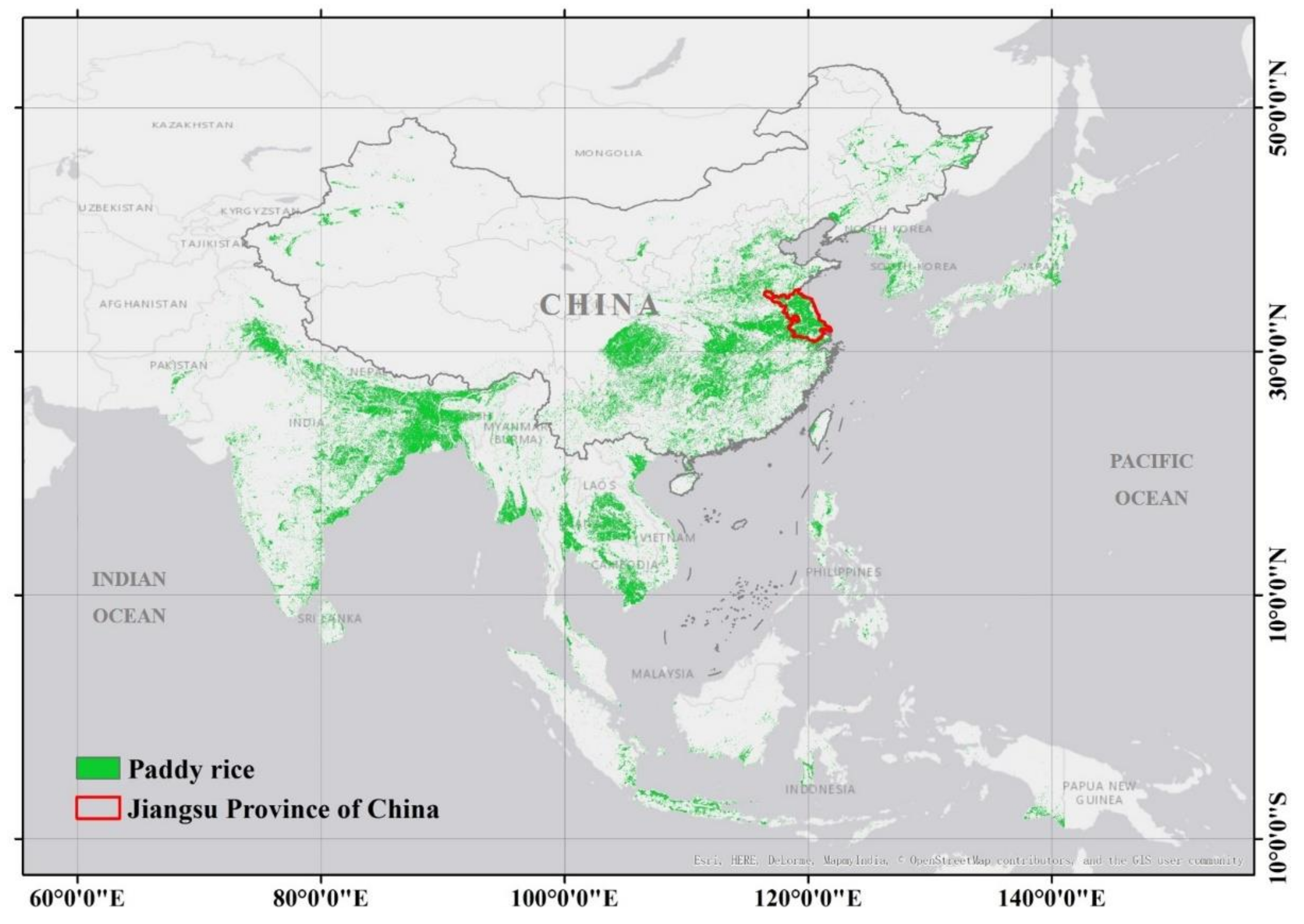
According to the 500-m resolution paddy rice map of monsoon Asia [37], Jiangsu Province of China is one of the most concentrated rice planting regions worldwide. As one of the wealthiest provinces in China, Jiangsu is experiencing the rapid development of various industries and urbanization against the preservation of farmland from limited resources. Under these circumstances, Jiangsu represents an ideal research area for rice mapping research with Landsat imagery. Therefore, the objectives of this study were (1) to evaluate the classification performance of OCSVC for rice mapping against other classification methods (MCSVC, DTC and VIT); (2) to assess the accuracy in county-level estimation of rice acreage with OCSVC and traditional methods; and (3) to generate a rice map for the whole province of Jiangsu.

2. Materials and Methods

2.1. Study Area

Jiangsu Province is located in the eastern coastal region of China and in the lower reach of the Yangtze River. It covers an area of 107,200 km², accounting for 1.1% of the total area of the country. Its rice cultivation area occupies 7.5% of the total area of China [6]. Jiangsu has two of China’s largest freshwater lakes—Taihu Lake and Hongze Lake—in the territory [38]. Mild climate and moderate rainfall make Jiangsu Province one of the most suitable regions for rice planting among the major rice cultivation areas in the world (Figure 1).

According to the Statistical Yearbook of Jiangsu [38], rice, corn, soybean, and peanut are the main cultivated crops during the summer season. Rice planting area was 22,948 km², followed by corn (4442 km²), soybean (2017 km²), and peanut (939 km²).

Table 1. Growth duration of summer crops in Jiangsu Province.

	April	May	June	July	August	September	October
Rice		Sowing	Emergence			Senescence	Harvest
Summer corn				Sowing & Emergence		Senescence	Harvest
Soybean		Sowing	Emergence			Senescence	Harvest
Peanut	Sowing & Emergence					Harvest

shows the growth duration of these four crops separately. Due to the local cultivation practices, corn, soybean, and peanut are mainly concentrated in the northern region and seldom appeared with large field plots in the southern region.

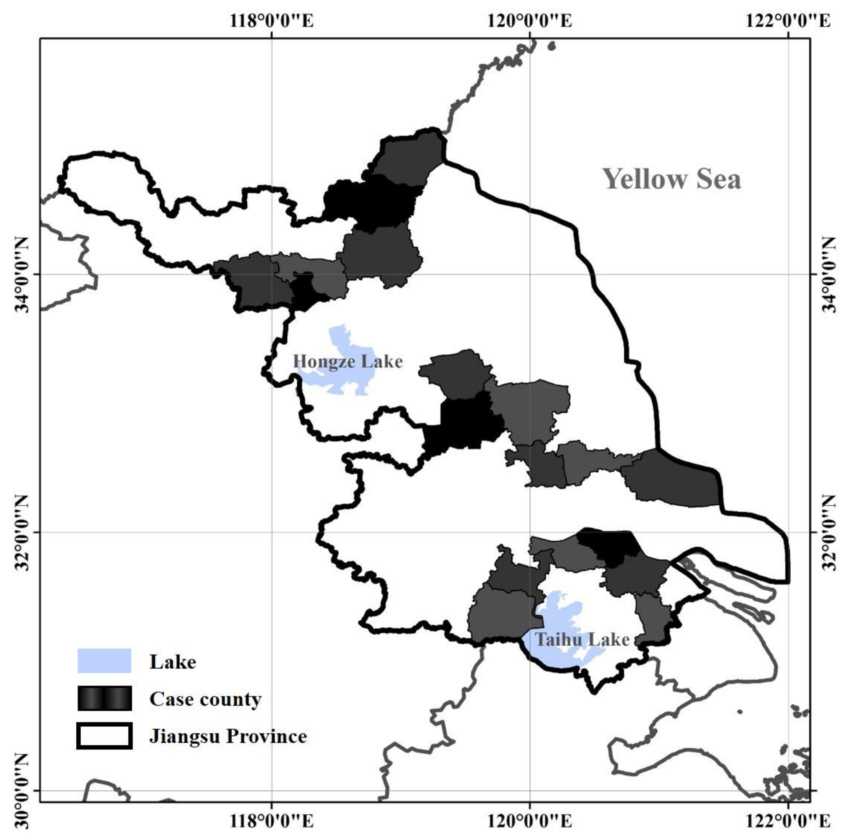
According to administrative planning and cultural characteristics, the whole province is divided into southern, central, and northern regions. The northern, central, and southern parts of Jiangsu contain different terrain, planting structure, and urbanization levels. Northern Jiangsu is characterized by the largest area of cultivated crops and the greatest diversity of crops types. Central Jiangsu is characterized by well-connected river systems and hydrological networks where rice is the most cultivated crop. Central and southern parts have more rainfall than the northern part. In addition to the rivers and lakes, high-level urbanization leads to smaller and scattered fields in the southern region. Six typical counties were selected from each of the three regions (Figure 2) to evaluate the proposed classification method. In each region, the typical county set was decided by selecting six neighboring counties from the coast to the inland border of the province. Only counties with greater than 60 km² of rice acreage in recent years were selected to represent major rice production areas. The three sets of counties are disconnected from each other and could represent the growing conditions, land cover variation, and rice planting patterns across the province.

2.2. Imagery Data

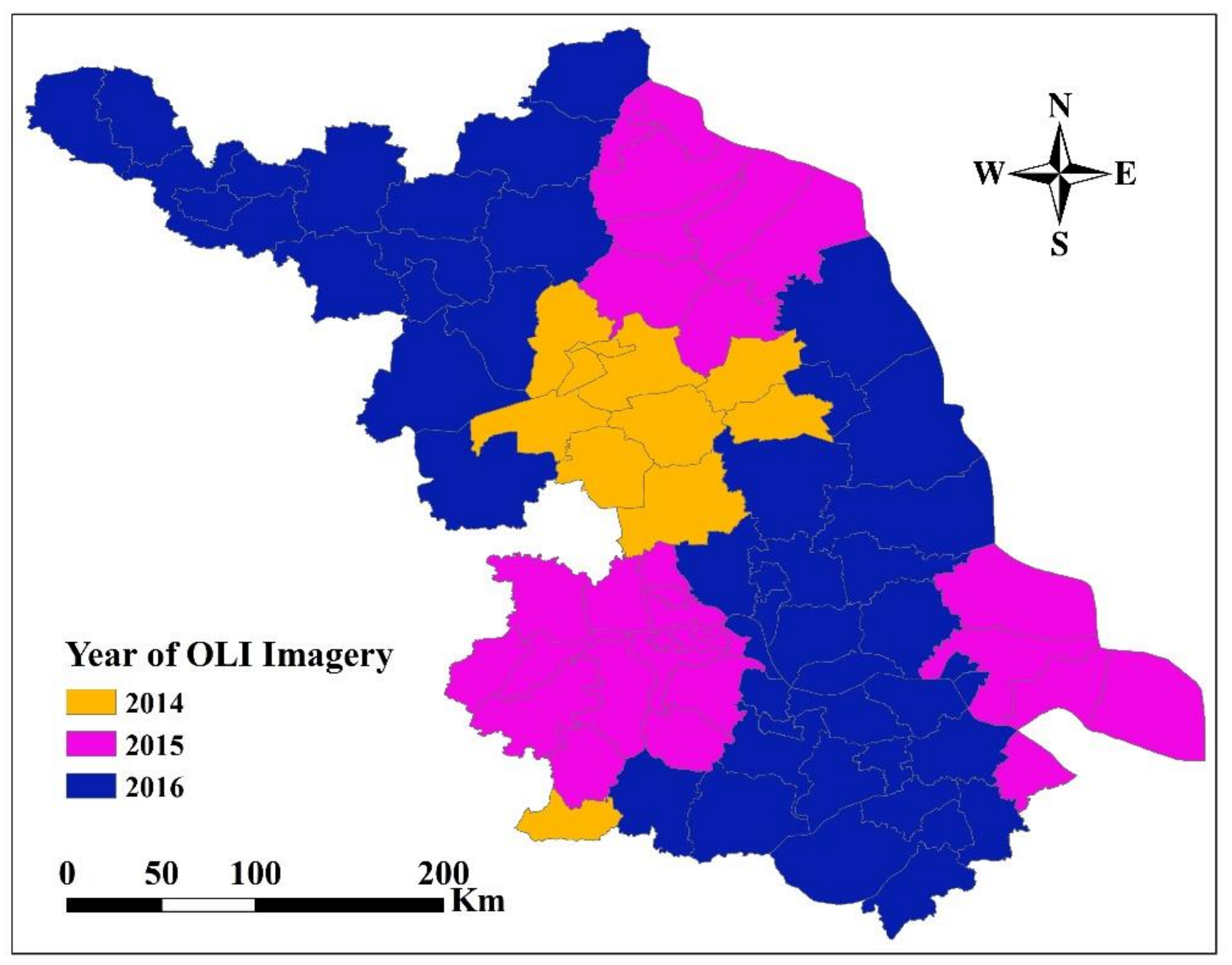
In addition to carrying out the comparison between four classification methods among the case counties, we would then use OCSVC to generate a distribution map of paddy rice for the entire province. High-quality satellite images which could cover the entire province were acquired for this purpose. All imagery data used in this study were from Landsat 8 Operational Land Imager (OLI). The rice growing season in Jiangsu Province often exhibits a long period of rainy days, which precludes the availability of complete time series Landsat imagery. To avoid the inadequacy of cloudless images from one year, we used images acquired in the last three consecutive years. This strategy is supported by the marginal variation in total rice cultivation area in three recent years. According to the Statistical Yearbook of Jiangsu [38], the total rice area of 2016 is 22,948 km², which is only 0.14% higher than that of 2015 (22,916 km²) and 1.02% higher than that of 2014 (22,717 km²). For the purpose of generating a provincial rice map of year 2016, the cloudless OLI imagery acquired in 2014, 2015, and 2016 was used (Figure 3). A total of 17 OLI images were downloaded from USGS EarthExplorer data portal [39]. All images are level-2 Surface Reflectance data generated from the Landsat Surface Reflectance Code (LaSRC). All images were limited to the time window from the late tillering stage to the late filling stage of the year and represented the highest data quality in terms of cloud cover (

Table 2. A list of Landsat OLI images used in this study.

NO.	Path-Row	Date	Field Campaign Date	Phenological Stage
1	118-038	03/08/2015	/	Vegetative stage (jointing)
2	119-037	27/09/2015	/	Ripening stage (filling)
3	119-037	28/08/2016	08/10/2016	Reproductive stage (heading)
4	119-038	27/09/2015	/	Ripening stage (filling)
5	119-038	28/08/2016	26/09/2016	Reproductive stage (heading)
6	119-039	27/07/2016	29/09/2016	Vegetative stage (tillering)
7	120-036	18/09/2015	/	Ripening stage (filling)
8	120-036	20/09/2016	04/10/2016	Ripening stage (filling)
9	120-037	01/10/2014	/	Ripening stage (filling)
10	120-037	02/09/2015	/	Reproductive stage (heading)
11	120-037	18/09/2015	/	Ripening stage (filling)
12	120-037	20/09/2016	05/10/2016	Ripening stage (filling)
13	120-038	29/07/2014	/	Vegetative stage (jointing)
14	120-038	02/09/2015	/	Reproductive stage (heading)
15	121-036	25/07/2016	06/10/2016	Vegetative stage (tillering)
16	121-037	25/07/2016	07/10/2016	Vegetative stage (tillering)
17	122-036	02/09/2016	/	Reproductive stage (heading)

). The images from beyond the period were not used because the rice plants were too weak in their spectral signature at earlier stages and might be harvested in some areas at later stages.

An obvious feature of rice cultivation is that rice grows in water-covered soils [40]. Only using multi-spectral bands may not be able to take full advantage of the relationship between remote sensing variables and rice growing background. Hence, this study introduced the brightness, greenness, and wetness (BGW) bands generated by Tasseled Cap Transformation (TCT) into the classification.

Table 3. TCT coefficients for Landsat 8 reflectance data.

	Band 2	Band 3	Band 4	Band 5	Band 6	Band 7
TCT	(Blue)	(Green)	(Red)	(NIR)	(SWIR1)	(SWIR2)
Brightness	0.3029	0.2786	0.4733	0.5599	0.508	0.1872
Greenness	−0.2941	−0.243	−0.5424	0.7276	0.0713	−0.1608
Wetness	0.1511	0.1973	0.3283	0.3407	−0.7117	−0.4559

Note: NIR = near-infrared, SWIR = shortwave infrared.

shows the bands and transformation coefficients for Landsat 8 reflectance data [41]. Brightness and greenness bands were used to reveal the spectral information of soil and vegetation in paddy fields. The wetness band was used to enhance the water background feature of paddy fields. With inclusion of these three bands, we could make better use of the characteristics of rice growing background to distinguish rice from other vegetation types.

2.3. Field Data

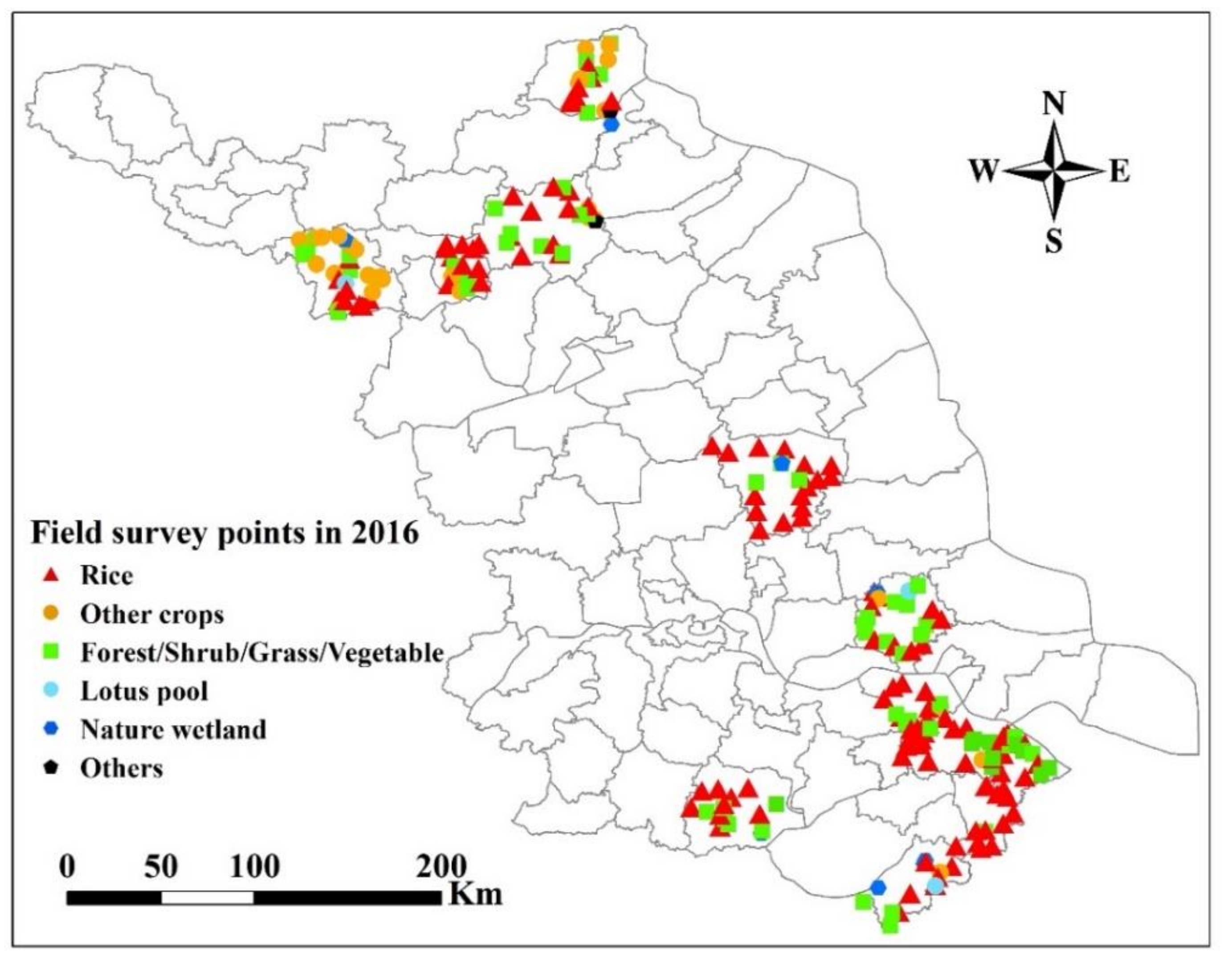
To verify the land cover types, we conducted a field campaign in Jiangsu Province during the ripening period in 2016 (Figure 4). We designed the routes using high spatial resolution Baidu Maps and county road maps before surveys. The routes were determined according to the territories of counties that are scattered in Northern, Central, and Southern parts of Jiangsu Province. Along the survey routes, we collected random field points at sub-pixel locations. We obtained precise coordinates using GPS and took photos at corresponding sites. Photos were taken inside the fields at a distance of 30 m or more away from the field boundaries using digital cameras. To ensure the land cover types could be re-confirmed after the survey, we took at least eight photos in eight directions within each field. Some extra photos were taken from other positions nearby in order to better describe the surroundings. A total of 227 points with 2170 photos were collected during the field campaign in 2016, including points for paddy rice, other crops (corn, soybean and peanut), natural wetlands, forests, and shrubs.

According to the field survey on the basis of planting practices and land use conditions, we found 14 major land cover types across the entire province and then defined them for the MCC methods. They were rice, forest, greenhouse vegetation, grass or vegetables, shrub, soybean, corn, peanut, tea, lotus, aquatic vegetation, built-up land, water body, and barren land. Eleven of these categories contained the spectral features of vegetation. Aquatic vegetation contained floating plants, helophyte, and waterside vegetation.

Polygons of interest (POIs) were extracted from OLI imagery using visual interpretation with the help of field survey data and very high resolution images, such as GF-1, GF-2, Pléiades, and Google Earth imagery. We converted the coordinate-tagged field locations into POIs in ArcGIS. With reference to high spatial resolution images. We then used a vector creating tool to draw around or near the POIs which were covered by the same land use types, as determined by reference field photos. All the POIs were used to form training and validation sets for the classification methods. A total of 2826 POIs comprising 200,655 pixels were generated for training, including 1332 POIs (88,381 pixels) for paddy rice and the rest for other land cover classes (

Table 4. Training and validation samples (represented by POI/pixel number) used in this study.

Training Set			Validation Set
Class	County and Province Level		Class	County Level (All Four Methods)	Province Level (OCSVC)
	MCC	OCC
Rice	1332/88,381	1332/88,381	Rice	1206/64,218	834/44,786
Forest	272/11,288	0	Non-rice	1494/77,530	819/45,974
Greenhouse vegetable	35/688	0
Grass or Vegetables	114/5391	0
Shrub	13/511	0
Soybean	153/4166	0
Corn	59/2177	0
Peanut	4/153	0
Tea	5/87	0
Lotus	9/886	0
Aquatic vegetation	193/7732	0
Built-up land	223/22,235	0
Water body	280/55,894	0
Barren land	37/1066	0

Note: MCC stands for MCSVC & DTC and OCC stands for VIT & OCSVC.

). In addition, 64,218 pixels for rice and 77,530 pixels for non-rice were prepared for the validation of county-level classification accuracy. At the province level, an additional validation dataset with evenly-distributed points across the province included 44,786 pixels for rice and 45,974 pixels for non-rice classes.

2.4. Classification Methods

In this paper, we proposed to map the paddy rice planting area using the one-class support vector classification (OCSVC) method. In addition, we conducted multi-class support vector classification (MCSVC), decision tree classification (DTC), and vegetation index thresholding (VIT) for the same case counties. We classified the rice planting area using OCSVC for the whole province to evaluate its stability and applicability at a large scale.

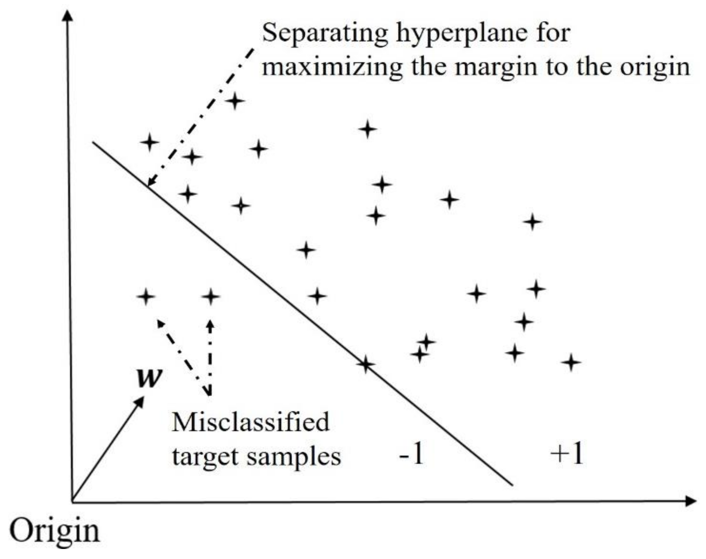
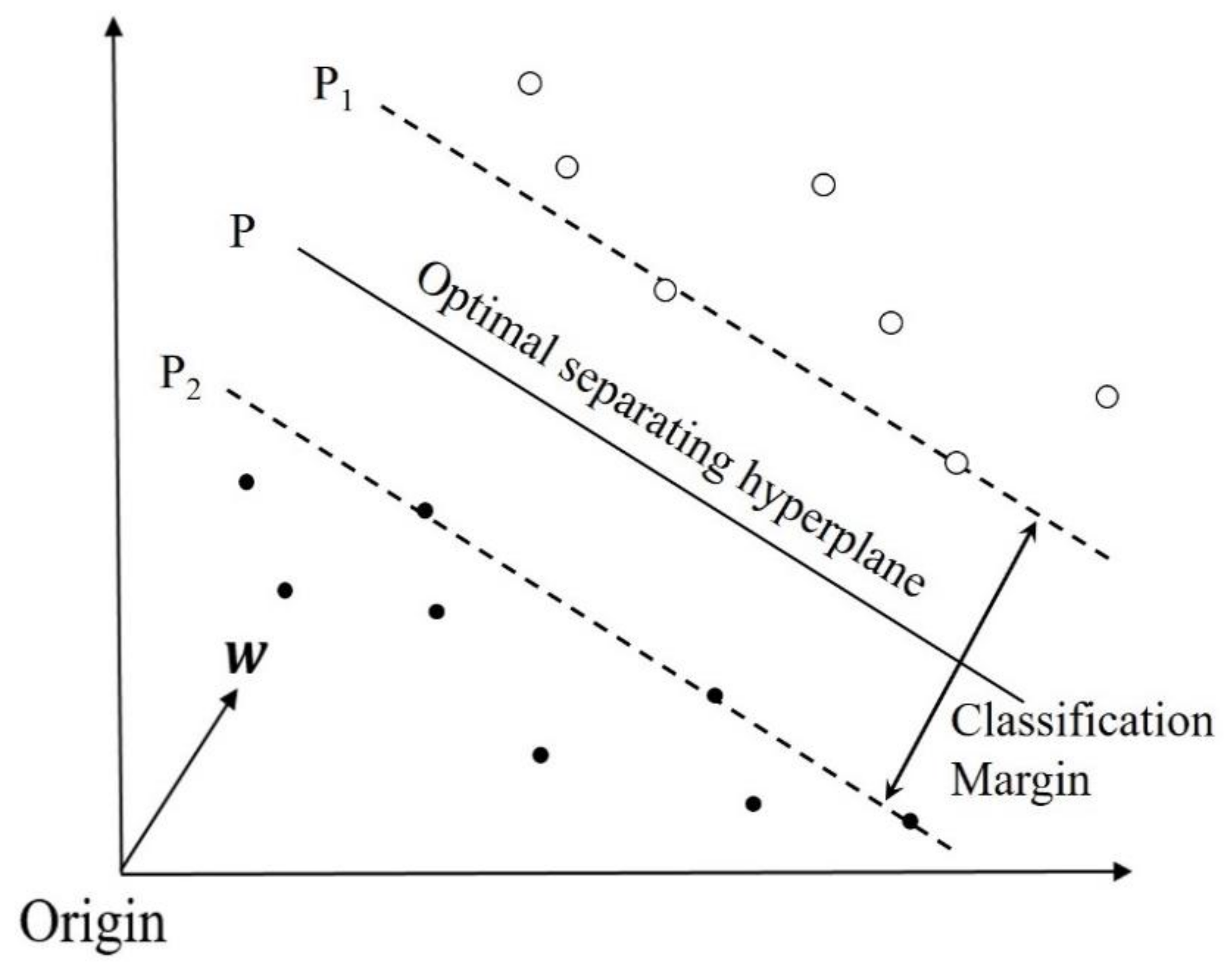
OCSVC is a particular type of support vector classification [42] and also a popular one-class classifier. It was developed to handle one-class classification (OCC) cases [43] where only the target class matters and needs to be trained [44,45]. The OCSVC algorithm first maps training data into a high-dimensional feature space. With support vectors and a kernel function, OCSVC is supposed to generate the maximal margin hyperplane, which could maximally separate the training data from the origin (Figure 5). The separating hyperplane can be represented with the function:

$$f\left(x\right)= 〈x,\mathit{w}〉+ b.$$

(1)

In this formula, $\mathit{w}$ is the normal vector and $b$ is a bias term. The function can be briefly described by labelling a test sample x. If $f\left(x\right)$ is greater than 0, then x would be labeled as a normal (target class). Otherwise, it would be labeled as an anomaly (outlier class).

Multi-class support vector classification (MCSVC) is a powerful machine learning methodology for land cover mapping [46] and also one of the most popular multi-class classification (MCC) methods. The basic idea of MCSVC can be illustrated in Figure 6 by taking the two-class classification as an example. The solid points and the hollow points represent two different classes of samples in a high-dimensional feature space and P is the optimal separating hyperplane. P1 and P2 are the hyperplanes generated by two classes of support vectors, both paralleling to P. The distance between P1 and P2 is called the classification margin. The optimal separating hyperplane P separates the two categories by maximizing the classification margin.

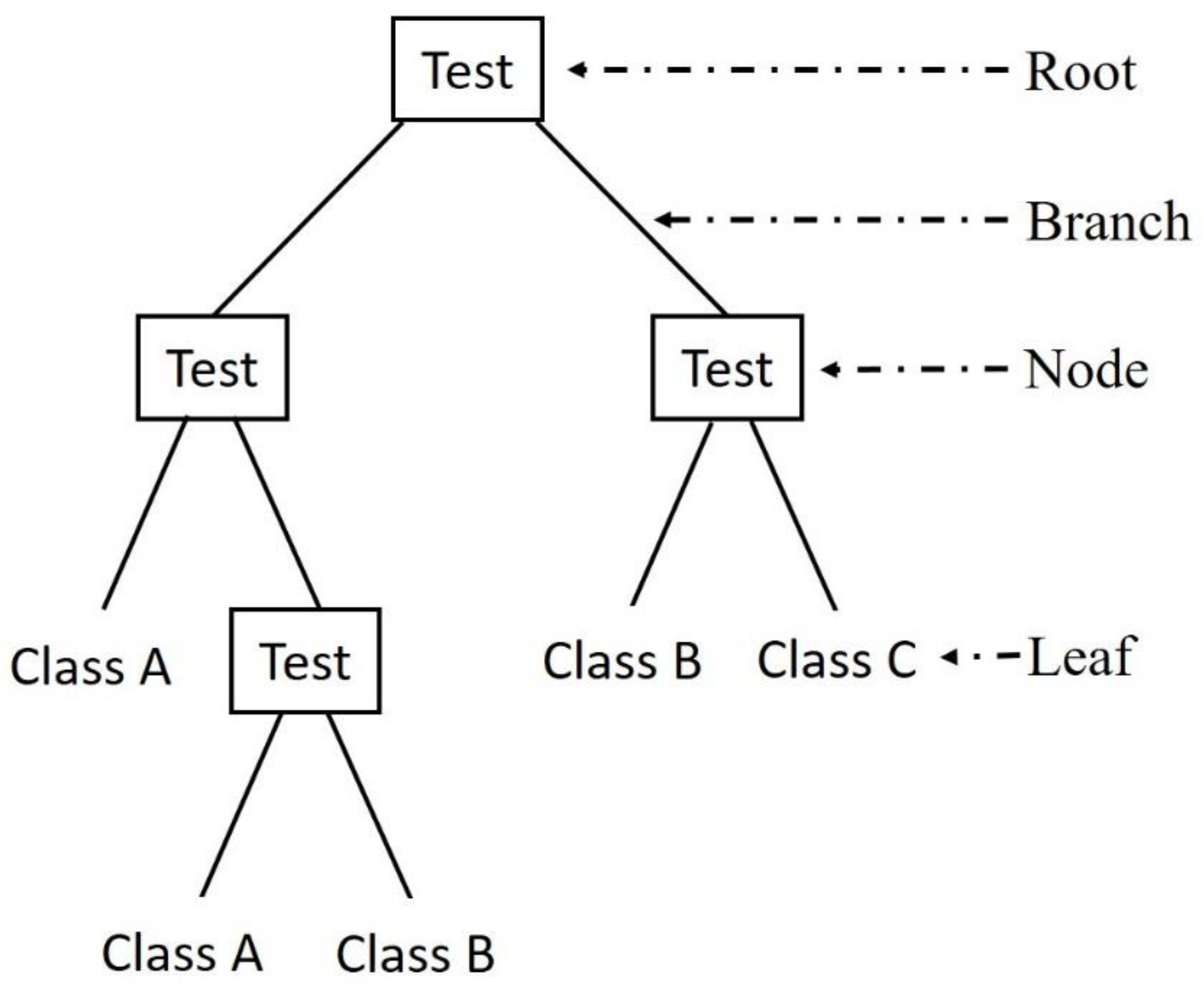
DTC is another widely-used MCC algorithm for land cover classification with remotely-sensed data [47]. By training known samples and summing up rules from the training process, the DTC establishes a tree structure (Figure 7). The tree connected by sets of branches and nodes can be used to classify the whole dataset (root node) into different classes (leaf nodes). Each internal node in a decision tree represents a test of an attribute, while each branch stems from one parent node and leads to two descendant nodes. Each descendant node represents a possible value of this attribute, or a gathering of many possible values. Finally, each leaf node corresponds to a resultant category.

The vegetation index used in our VIT method was Normalized Difference Vegetation Index (NDVI) [48]. The VIT only needs the NDVI histogram of the target-class training set and an empirical percentage (δ) to decide the thresholds [49]. If the NDVI value is out of head and tail percentages determined by the thresholds, the pixel is excluded. The target class can be simply extracted from the entire dataset when the NDVI meets the condition.

In this rice mapping study, the objective was to extract the rice planting area and leave other land cover types alone. Therefore, only training samples of rice were defined and sampled for OCSVC. For the two MCC methods, all categories were strictly defined and sampled. For MCSVC and DTC, all kinds of vegetation types were separated precisely since our target type is only one of them. For VIT, the δ was taken as 0.01 so that the NDVI values that give probability density equal to 1% and 99% were determined as the classification thresholds. The thresholds were calculated among 18 case counties, respectively. It is necessary to point out that the MCSVC shared the same multi-class training sets with the DTC. Meanwhile, the four methods evaluated in this study shared the same set of training samples of rice.

2.5. Evaluation of Classification Accuracy

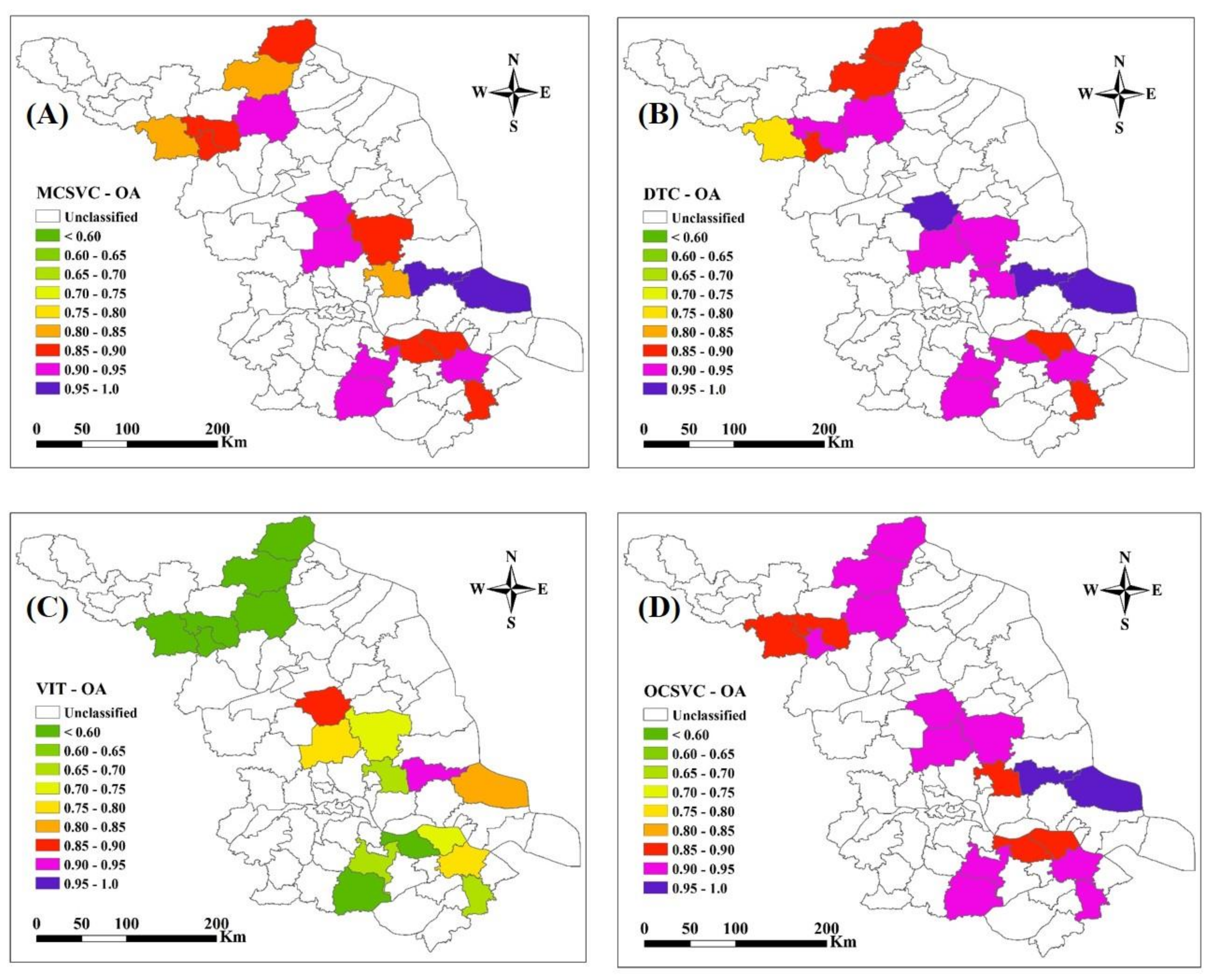
The classification results of two MCC methods would be reclassified into rice and non-rice class to carry out the accuracy test since OCC methods only produce results of these two classes. The POIs for validation were also divided into two classes (rice and non-rice) and used to assess the location accuracy of the resultant rice maps using confusion matrix. The non-rice class was mainly composed by non-rice vegetation in order to test the paddy field recognition ability of the four methods. Information in the confusion matrix can be evaluated using simple descriptive statistics, such as producer’s accuracy (PA), user’s accuracy (UA), overall accuracy (OA), and the kappa coefficient.

The validation of classification accuracy was conducted at county level and province level, respectively. At the county level, the confusion matrix was performed by taking 18 case counties in their entirety and for every county. We compared the classification performance between the four methods in PA, UA, OA, and kappa coefficient. We also calculated the mean value, standard deviation, and coefficient of variation (CV) of the OAs over the 18 counties to compare the stability of each method. At the province level, the resultant rice map was evaluated with the provincial validation dataset through a confusion matrix as well.

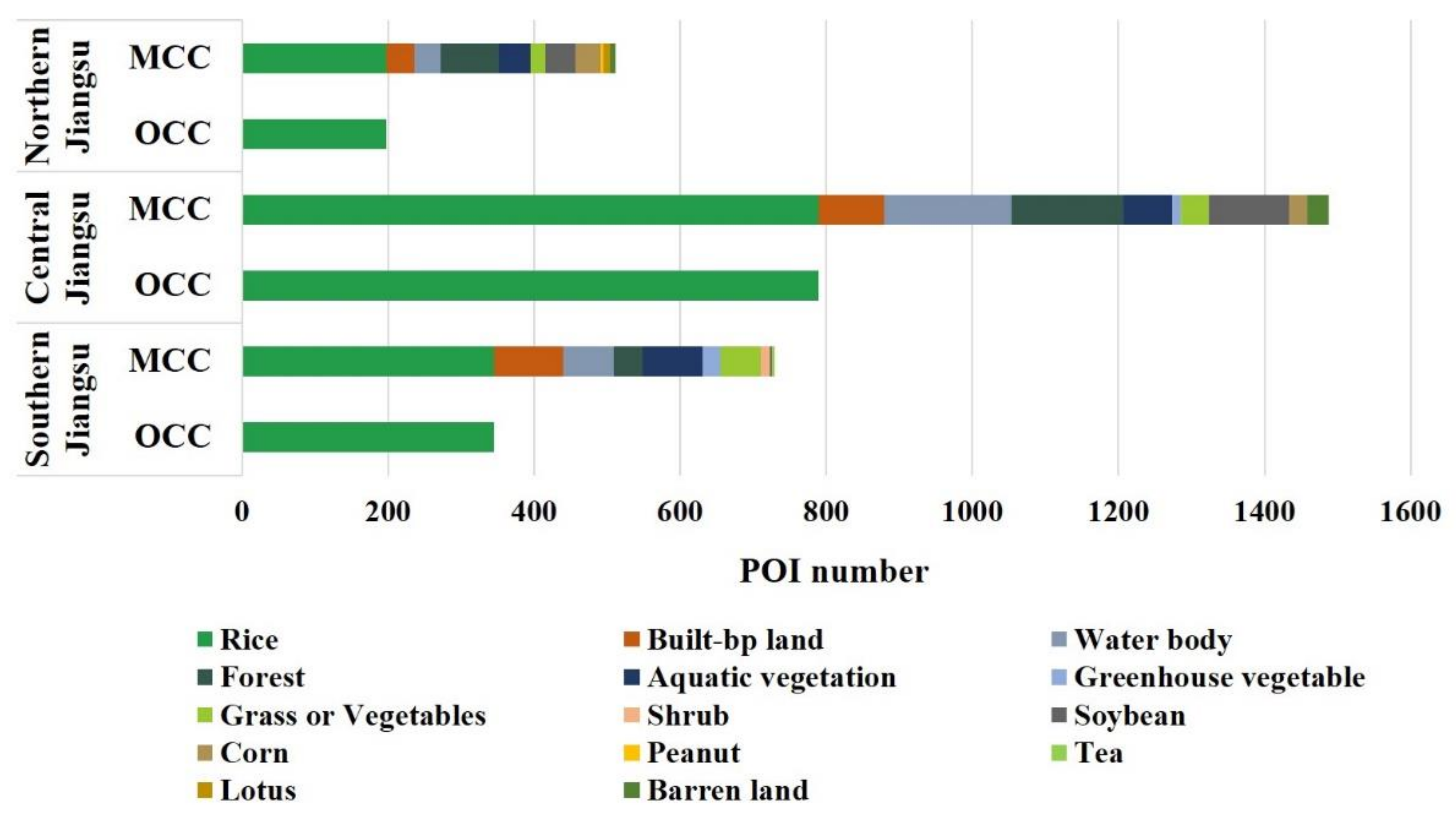
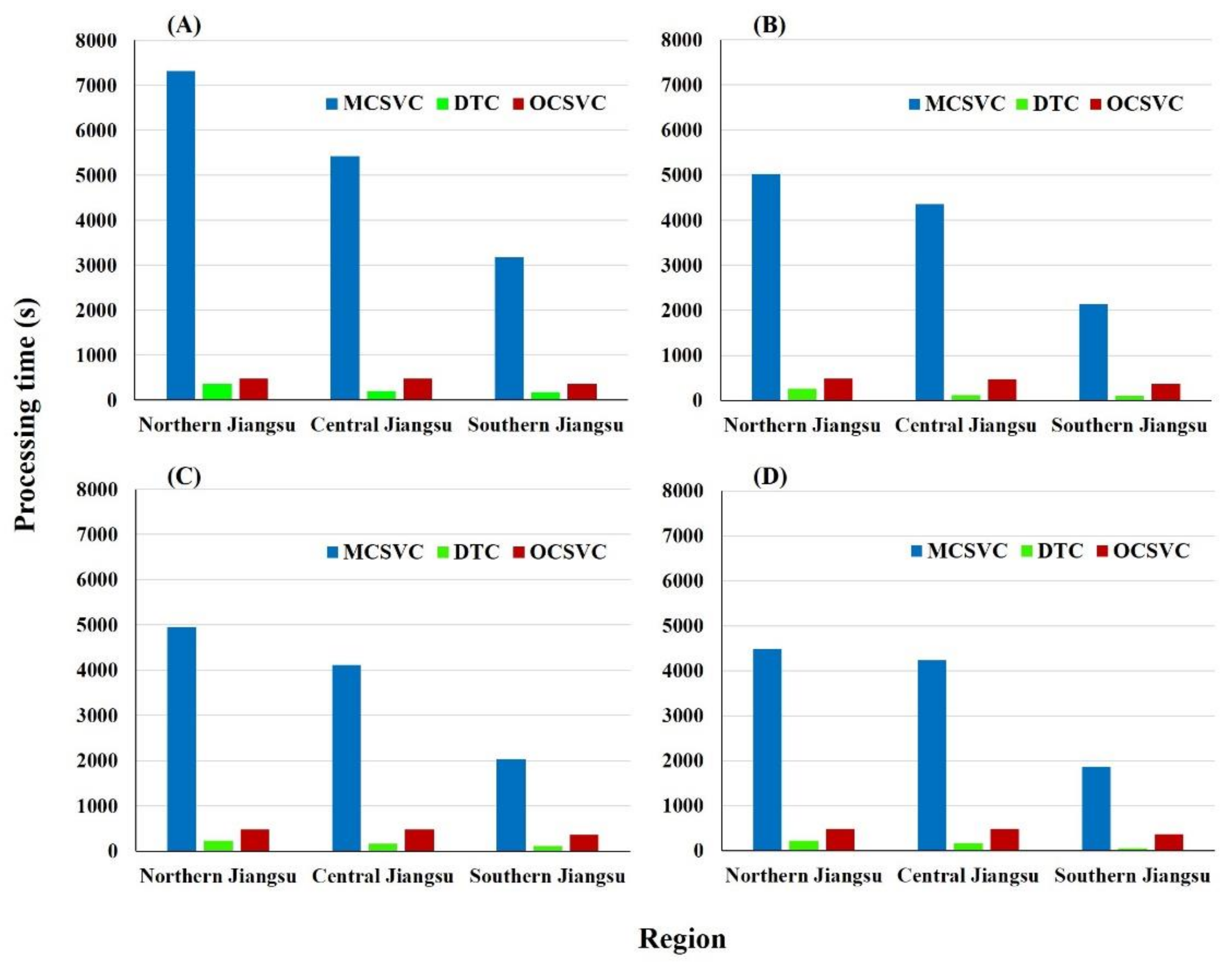
2.6. Evaluation of Classification Efficiency

We compared the labor cost and time consumption between the four methods to evaluate the classification efficiency. The size of training set was regarded as the labor cost. We used the POI number to represent the size of training samples.

The time consumption of classification covered the establishment of the classification model and the process of image classification. Since VIT only needed time for determining thresholds, its time consumption was ignored. To exclude other variables, we designed four groups of tests to better assess the processing time of different methods. In addition, the 14 classes of training samples were reorganized into four classes, three classes, and two classes to investigate the influence of class definition on the computational time.

The first group contains all 14 classes. The four classes in the second group were rice, non-rice crop, non-crop vegetation, and non-vegetation. The three classes in the third group were rice, non-rice vegetation, and non-vegetation. The two classes in the fourth group were rice and non-rice. All the training samples were redistributed from the original 14-class training dataset so that each group corresponded to the same training pixels. It should be noted that the reprogramming reorganization of training classes was only used to analyze its influence on the classification efficiency, rather than on the classification accuracy.

2.7. Assessment of Rice Acreage Estimation

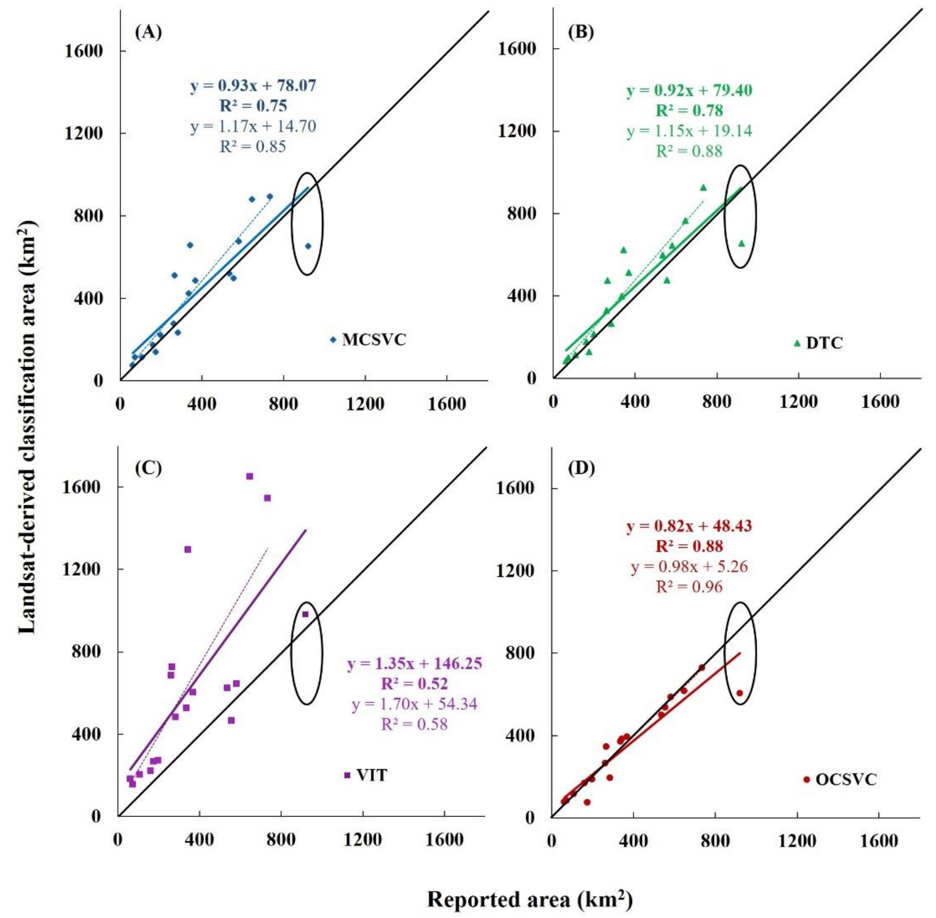
To assess the area accuracy of our rice planting area extraction method, we compared the reported rice acreage to our classified rice area. The statistical data of rice cultivation area in 2016 for all counties of the province were cited from agricultural department report [50]. At the county level, the correlation between two sets of data was evaluated using the coefficient of determination (R²), the root mean square error (RMSE) and the bias (Bias) calculated as:

$$R^2=1-\frac{{{\displaystyle \sum }}_i{\left(y_i-y_i^{\prime }\right)}^2}{{{\displaystyle \sum }}_i{\left(y_i-\overline{y}\right)}^2},$$

(2)

$$RMSE=\sqrt{\frac{{{\displaystyle \sum }}_i{\left(y_i-y_i^{\prime }\right)}^2}{n}},$$

(3)

$$Bias=\frac{{{\displaystyle \sum }}_i\left(y_i-y_i^{\prime }\right)}{n},$$

(4)

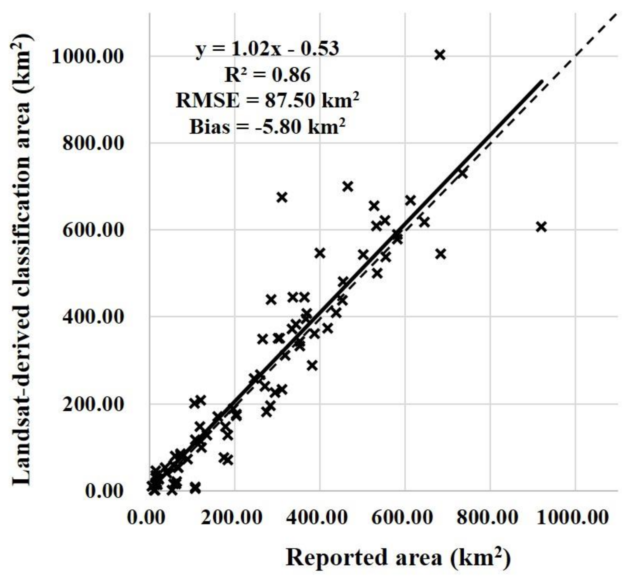
where $y_i$ and $y_i^{\prime }$ are the reported and classified acreage for county $i$, $\overline{y}$ is the arithmetic mean of classified acreage, and $n$ is the number of counties. At the province level, the rice cultivation area data from the statistical department in 2016 [38] was acquired to evaluate the area accuracy of the provincial rice map.

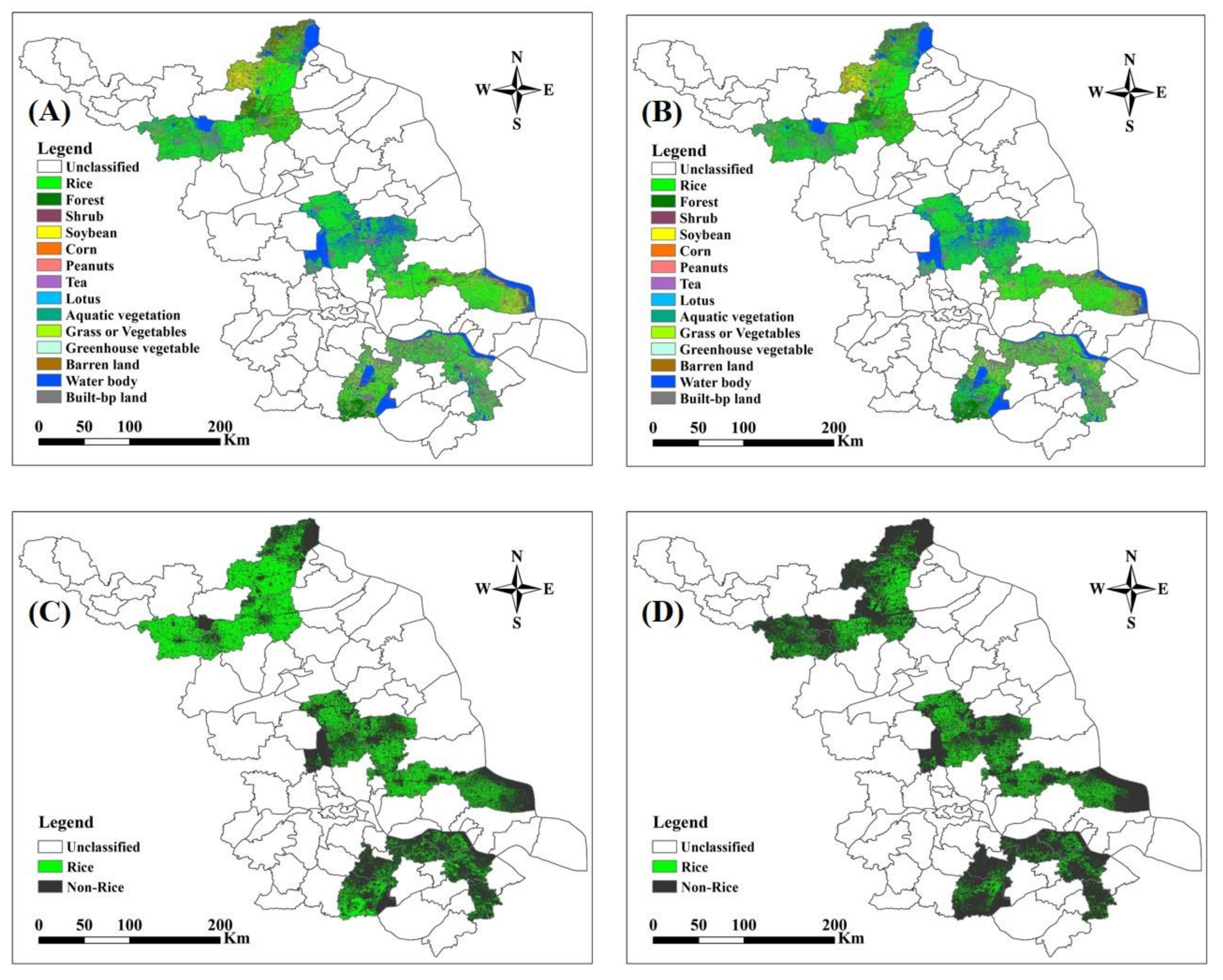
3. Results

3.1. Classification Accuracy

Table 5. Comparison of classification performance between the four methods.

Classifier	Producer’s Accuracy (%)	User’s Accuracy (%)	Overall Accuracy (%)	Kappa Coefficient	OAmean (%)	OAstd (%)	CV(%)
MCSVC	95.63	83.85	89.68	0.79	89.27a	5.10	5.71
DTC	95.52	87.05	91.53	0.83	91.25a	4.31	4.73
VIT	96.65	57.63	66.3	0.36	64.96b	15.97	24.59
OCSVC	89.87	90.52	91.15	0.82	91.36a	2.79	3.05

Note: The coefficient of variation (CV) is calculated upon OAs of 18 case counties. OA_mean and OA_std are the mean and standard deviation of overall accuracies over the 18 counties. The number in bold denotes the best performance in each column. Values per classifier in OA_mean column followed by letters a and b indicate the significant difference between classifiers, while the same letters indicate no difference at the 0.001 probability level.

summarizes the classification accuracies for the identification of paddy fields over 18 case counties using the four methods. The classification accuracies with DTC (OA = 91.53%, kappa = 0.83) and OCSVC (OA = 91.15%, kappa = 0.82) were marginally different. They were slightly higher than that with MCSVC (OA = 89.68%, kappa = 0.79) and remarkably higher than that with VIT (OA = 66.30%, kappa = 0.83). With regard to Producer’s accuracy, VIT performed the best and was closely followed by MCSVC, DTC and OCSVC. In terms of User’s accuracy, a significant contrast was seen among methods with OCSVC being the highest (UA = 90.52%) and VIT being the lowest (UA = 57.63%). The statistics of individual OAs for the 18 case counties showed the mean of OAs for OCSVC was not significantly different from those for MCSVC and DTC, but significantly higher than that for VIT.

Figure 8 shows the rice maps of these 18 counties with four classification methods. The two multi-class classification maps with MCSVC and DTC both have rice as the dominant class and generally exhibit the same spatial pattern in rice planting area. VIT captured the maximum rice planting extent among four methods, while OCSVC captured the minimum.

Figure 9 represents maps of the county-level classification overall accuracy for the four classification methods. Generally, the OA map for OCSVC (Figure 9D) is more uniform than the other three maps (Figure 9A–C). VIT exhibited the most significant variation among counties, with the lowest OAs for the northern counties and the greatest contrast for the middle counties. With the other three classification methods, the between-county difference in OA was the most insignificant for the northern counties.

3.2. Efficiency Comparison between OCSVC and Other Classification Methods

While the two multi-class classifiers MCSVC and DTC needed samples from all of the fourteen land cover classes for training, VIT and the one-class classifier OCSVC needed samples only from the target rice class. Additional samples required for the non-rice classes could be as much as those from the rice class (Figure 10) and doubled the effort on training data collection. The northern counties needed the fewest training samples (counted as the POI number) and the middle counties needed the most, both for the rice class and the non-rice classes.

Regardless of the location of case counties, MCSVC needed as much as ten times more computational time for classification than OCSVC and DTC (Figure 11). DTC was more efficient than OCSVC, but the difference in classification efficiency was substantially less significant. With the reduction of training classes, the computational time declined for MCSVC and DTC. For OCSVC, the computational time remains unchanged since only one class is needed all the time. The ranking of processing time for MCSVC, DTC, and OCSVC was the same for the four groups of class definitions.

3.3. County-Level Estimation of Rice Acreage

When comparing the county-level planting area from classification maps to the area from the statistical report, VIT produced the weakest correlation (R² = 0.52, p < 0.001) and serious overestimation (RMSE = 420.43 km², Bias = −275.45 km²) (Figure 12). The correspondence between the classified area and reported area was significantly better when using MCSVC (R² = 0.75, p < 0.0001) or DTC (R² = 0.78, p < 0.0001). These two classification methods also generated close regression models for the correlations. The match was even further improved using OCSVC (R² = 0.88, p < 0.0001). Most of the data points corresponding to MCSVC, DTC and OCSVC were found to be above or surrounding the 1:1 line. The errors for MCSVC (RMSE = 139.97 km², Bias = −53.54 km²) and DTC (RMSE = 127.17 km², Bias = −49.52 km²) were greater than that for OCSVC (RMSE = 84.68 km², Bias = 19.18 km²). All these three methods showed consistent underestimations for one data point, which was obviously below the line at the higher end. Excluding this outlying data point led to poorer fits to the 1:1 line for MCSVC (R² = 0.85, p < 0.0001) and DTC (R² = 0.88, p < 0.0001) but a better fit for OCSVC (R² = 0.96, p < 0.0001) (

Table 6. Assessment of accuracy for rice acreage estimation with the four classification methods.

Classifier	All Counties			One Excluded
	R2	RMSE (km2)	Bias (km2)	R2	RMSE (km2)	Bias (km2)
MCSVC	0.75	139.97	−53.54	0.85	128.87	−72.29
DTC	0.78	127.17	−49.52	0.88	114.21	−67.93
VIT	0.52	420.43	−275.45	0.58	432.37	−288.03
OCSVC	0.88	84.68	19.18	0.96	42.76	1.90

Note: The number in bold denotes the best performance in each column. All significance levels are at p < 0.001.

). Unlike for MCSVC and DTC, the mismatch for OCSVC was substantially improved and the error decreased to an RMSE of 42.76 km² and a Bias of 1.90 km².

3.4. Generation of the 2016 Provincial Rice Map of Jiangsu

Given the best performance among the four classification methods, OCSVC was used to generate a classification map of paddy rice for the entire province of Jiangsu (Figure 13). Rice fields could be seen across the whole province, but mainly in the central and northeast parts, particularly the Hongze Lake region and the northeastern coastal regions. The rice planting areas in the south and northwest parts were more heterogeneous and scattered by highly urbanized towns.

Figure 14 shows three representative sites in Northern, Central, and Southern Jiangsu, which provide more details on the identification of paddy fields at the field scale. Northern Jiangsu is characterized by the largest field sizes in the province and the Shuyang site exhibits the most homogeneous field patches on the classification map, as shown in Figure 14B,E. The rice paddy fields in Central Jiangsu, such as Gaoyou, are often separated by local rivers and ponds, which cause the dense cover of paddy rice to be broken by hydrological networks (Figure 14C,F). In addition to the rivers and lakes, the well-developed industry in Southern Jiangsu, particularly in Kunshan, has created sparse crop cover, irregular field shapes, and scattered distribution of rice paddy fields (Figure 14D,G). All these typical spatial patterns in rice planting across the entire province have been well captured by the classification maps generated with OCSVC.

The classification map was generated with an overall accuracy of 88.54% and a kappa coefficient of 0.77 based on the provincial validation dataset (

Table 7. The confusion matrix for the rice classification map obtained with OCSVC.

	Class	Ground Truth Pixels		Total Classified Pixels	User Accuracy (%)
		Rice	Non-rice
Classification	Rice	39,076	4689	43,765	89.29
	Non-rice	5710	41,285	46,995	87.85
Total validation pixels		44,786	45,974	90,760
Producer accuracy (%)		87.25	89.80
Overall accuracy (%)		88.54		Kappa coefficient = 0.77

). The total rice area derived from the provincial map through pixel counting was 22,602 km², which is 1.51% lower than the statistics from the National Bureau of Statistics (22,948 km²). Figure 15 shows a comparison of the reported acreage with the rice area identified with OCSVC for all counties of the province. This county-level comparison exhibited a strong correlation (R² = 0.86, p < 0.0001) between the two types of numbers and produced a regression trend closely tied to the 1:1 line. Most of the data points were scattered along the 1:1 line, except a few outlying points at the higher end.

4. Discussion

4.1. Misclassifications and Omissions in OCSVC Classification

Many studies have investigated the application of OCC methods to vegetation coverage change detection [45] and vegetation discrimination [32,34,51], but few of them paid attention to the misclassification and omission characteristics of those methods. The omission errors for rice mapping in this study were mostly observed in poorly-growing rice fields, mixed pixels at field boundaries [19] and late transplanting fields. This may be related to the lack of sufficient training pixels over the areas with ambiguity of class memberships. Collecting representative samples for those areas is challenging for the high-resolution imagery and requires considerably more effort for field surveys. When comparing the reported rice acreage to the classified rice area, one county exhibits remarkable underestimations for MCSVC, DTC, and OCSVC (Figure 12). The outlying county experienced a significant expansion of the fishery industry in recent years, which might have caused the confusion between rice planting and fishery uses for reporting.

The detection of rice pixels using OCSVC exhibited the lowest misclassification errors among all methods. Our experiment revealed that tree plantations in the forest class, floating plants in the aquatic vegetation class held the highest possibilities of being misclassified as rice among all non-rice categories. Similar to the rice paddies, the tree plantations were arranged regularly and had high vegetation coverage. The floating plants with high density and paddy rice were growing in the similar environment and, therefore, exhibited high spectral similarity. To reduce the misclassification errors, we had added brightness, greenness, and wetness (BGW) components to the OLI multispectral bands as input data for OCSVC. This inclusion was supported by the application of BGW to forest and rice detection [52,53]. The misclassification of mixed pixels at field boundaries may be addressed with soft classification methods that allow multi-class probabilities to be expressed on a pixel basis [54,55,56,57].

Apart from the confusion matrixes, no comparison in the areal extent was performed in this study due to the unavailability of suitable rice maps. The portion for Jiangsu in Figure 1 is available only at the spatial size of 500 m, which makes it difficult to compare with our rice map and evaluate the spatial mismatches. The large difference in spatial resolution led to large discrepancies in the areal extent. In addition, such a map at 30 m resolution is not yet available for China. Considering the interannual variation in planting practices, we may only be able to conduct a comparison when a reference map is available at the similar spatial resolution and timing of observation.

The influence of image acquisition timing on classification accuracies was not taken into account since sufficient cloud-free scenes over the growing season were unavailable. Cloudy or rainy weather conditions occurred often in the province and it was difficult to obtain enough high-quality image scenes within the season. This influence may be investigated in the future by adding images from other satellites, such as Sentinel-2.

While comparing the area values from remote sensing and official statistics, we chose to use absolute numbers (km²) rather than percentages (%) of rice area despite the size differences between counties. This was primarily because the ratios of rice area to county area would bring another potential source of error from county area statistics. Jiangsu is an economically dynamic province and the boundary changes frequently to the counties that are small, but located in the center of the upper level cities. Although there were size differences between the counties, the strongest regression for comparing classification area and reported area was obviously obtained for OCSVC (Figure 12). Compared to the percentages of rice area, the absolute rice areas would be more intuitive and convenient for understanding the misclassifications and omissions in OCSVC classification.

4.2. Advantages of OCSVC

This study evaluated the accuracy and efficiency of OCSVC for rice acreage estimation and extent mapping in comparison with other three traditional methods. The OCSVC method exhibited superior performance in area accuracy and operational efficiency (

Table 8. Comparison of the four classification methods by location accuracy, area accuracy, and efficiency.

Classifier	Location Accuracy		Area Accuracy	Efficiency
	Omission	Commission		Labor Cost	Time Cost
MCSVC	Lower	Low	Good	High	High
DTC	Lower	Low	Good	High	Low
VIT	Lower	High	Poor	Low	Negligible
OCSVC	Low	Lower	Good	Low	Low

). With regard to location accuracy, OCSVC did not exhibit significant differences from MCSVC and DTC for the mean of 18 case counties (Table 5). This suggests the use of OCSVC did not result in a loss of location accuracy from image classification at the price of increased computational efficiency and reduced training classes. The MCSVC and DTC performed well in accuracy evaluation but exhibited weaknesses in efficiency. The VIT was the most efficient method and identified the most complete set of rice pixels, but its high misclassification error and instability may pose significant problems in applications.

In terms of classification efficiency, one-class classifiers have obvious advantages in labor and time requirements. For OCSVC, training samples were only needed for the rice class. However, the multi-class classifiers DTC and MCSVC needed training samples from all the fourteen classes. The addition of non-rice classes led to the extra time cost in data collection and classification operation [58].

With regard to classification accuracy, OCSVC performed well in rice acreage estimation and achieved the best correlation with the official statistics. For VIT, the high degree of overestimation could probably be due to the high spectral similarity in NDVI between rice and other classes [25]. As the classes were defined on the basis of planting habits and known land use conditions, there are inevitably a few unusual land cover types that are lacking in definition for MCSVC and DTC. Even though we have conducted ground surveys for further verification, it is hardly possible to obtain perfectly representative training sets in large-scale classification studies. The confusion between underrepresented classes and the rice class led to the classification errors. However, such a problem did not happen to OCSVC because only the rice class needed to be defined.

Although the multi-class classification methods exhibited comparable location accuracy to OCSVC, the acreage estimated with OCSVC was best correlated with the official report data. This could be attributed to its stable performance over the whole study area rather than the validated locations alone. OCSVC is not sensitive to the diverse land cover patterns among counties when comparing to MCSVC and DTC. In addition, the pixels from the forest and aquatic vegetation classes tend to be misclassified as rice for OCSVC due to the lack of training data specifically for these two classes. The situation was better for the multi-class classifiers since these two classes were individually represented in the training data. This may explain why the performance of OCSVC was not well represented compared to the multi-class classifiers.

5. Conclusions

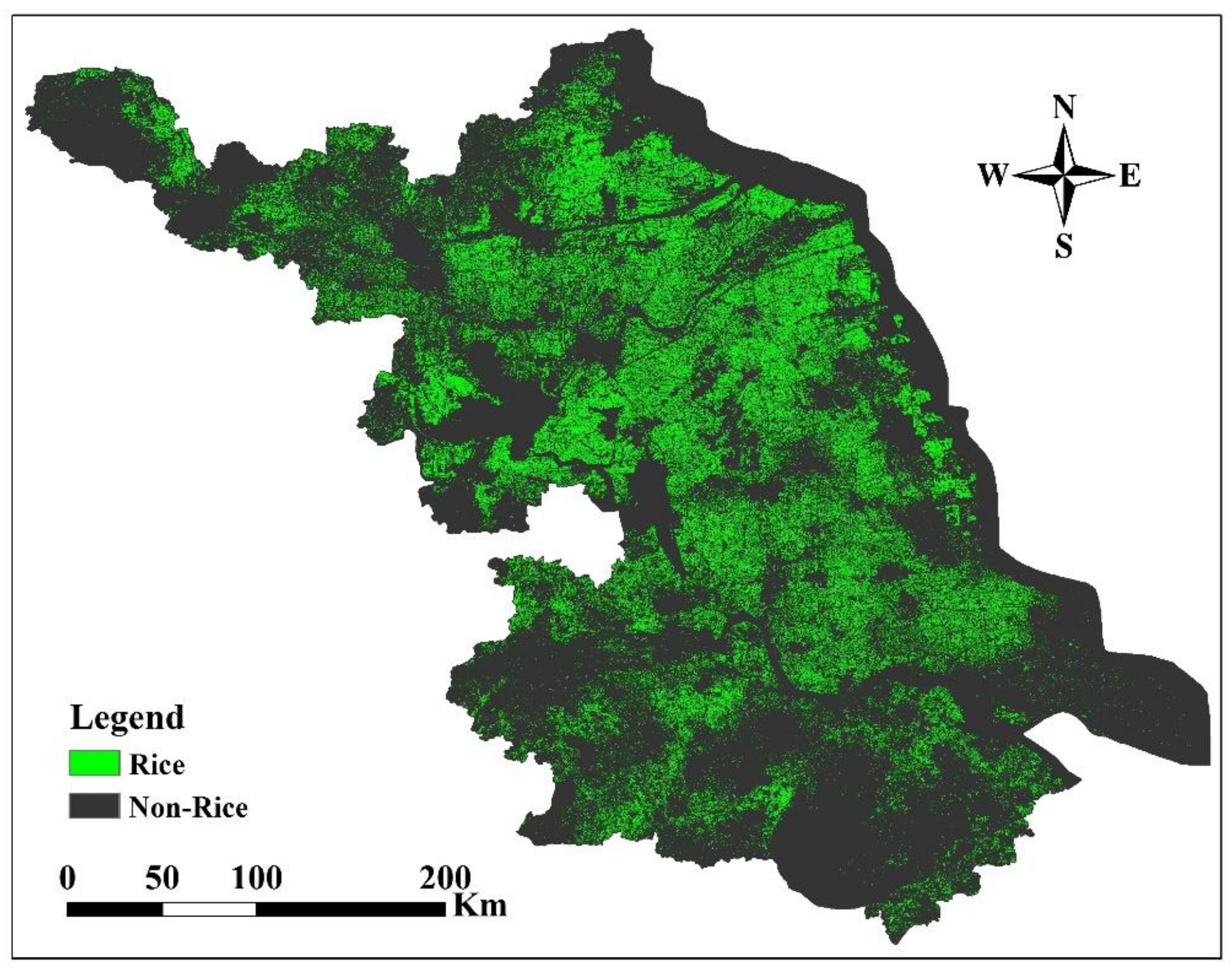
An OCSVC-based rice mapping method has been developed along with the 2016 provincial rice map of Jiangsu Province, China. Unlike the traditional rice mapping techniques, the OCSVC method only concentrated on the rice class. By resolving the distraction and inefficiency problem, the OCSVC provided a reliable and promising way for large scale rice mapping. For all of the 18 case counties, OCSVC produced an overall location accuracy (91.15%) comparable to that of DTC (91.53%) and outperformed MCSVC (89.68%) and VIT (66.30%). However, the computational efficiency increased approximately ten times with OCSVC being more efficient than MCSVC. In addition, OCSVC was more cost-effective because it only needed training samples from the rice class, but not the samples for the non-rice classes as required by the MCC methods MCSVC and DTC. The OCSVC achieved the best correspondence between its classified area and reported area with an R² at 0.88 comparing to MCSVC (R² = 0.75), DTC (R² = 0.78), and VIT (R² = 0.52). The planting area extracted from the 2016 rice map had a strong linear correlation with the official statistics from the provincial agricultural department and the overall accuracy for the provincial map was 88.54%. The detected rice planting area achieved a high accuracy which is only 1.51% lower than the statistics from the National Bureau of Statistics. In addition, the 30-m resolution rice map can better reveal the rice fields in detail compared to current rice maps of China.

Given the fact that variable land use types and cultivation patterns are the main difficulties for rice mapping in China, the proposed OCSVC provided a stable and efficient way to map rice extent with universal applicability. The resultant rice map of Jiangsu Province could serve as the base map for provincial-level crop monitoring and may be combined with grain yield data to forecast provincial rice productivity.

References

1. Brown, L.R. Who Will Feed China? Wake Up Call for A Small Planet; Norton and Company: New York, NY, USA, 1995. [Google Scholar]
2. Food and Agriculture Organization (FAO). How to Feed the World in 2050; FAO: Rome, Italy, 2009. [Google Scholar]
3. Dong, J.; Xiao, X. Evolution of regional to global paddy rice mapping methods: A review. ISPRS J. Photogramm. Remote Sens. 2016, 119, 214–227. [Google Scholar] [CrossRef]
4. Food and Agriculture Organization Corporate Statistical Database (FAOSTAT). Available online: http://faostat3.fao.org/faostat-gateway/go/to/home/E (accessed on 27 September 2017).
5. Kuenzer, C.; Knauer, K. Remote sensing of rice crop areas—A review. Int. J. Remote Sens. 2013, 34, 2101–2139. [Google Scholar] [CrossRef]
6. National Bureau of Statistics of China. China Statistical Yearbook 2017; China Statistics Press: Beijing, China, 2017.
7. Macdonald, R.B.; Hall, F.G. Global crop forecasting. Science 1980, 208, 670–679. [Google Scholar] [CrossRef] [PubMed]
8. Champagne, C.; McNairn, H.; Shang, J.; Johnson, D.M. Evaluation of Resoucesat-1 AWiFS data for producing an agricultural crop inventory for Canada. In Proceedings of the CRSS/ASPRS Specialty Conference: Our Common Borders-Safety, Security and the Environment Through Remote Sensing, Ottawa, ON, Canada, 28 October–1 November 2007. [Google Scholar]
9. Johnson, D.M.; Mueller, R. The 2009 cropland data layer. Photogramm. Eng. Remote Sens. 2010, 76, 1201–1205. [Google Scholar]
10. United Nations. Available online: http://www.un-spider.org/links-and-resources/data-sources/land-cover-map-globeland-30-ngcc (accessed on 3 March 2018).
11. USGS. Available online: https://geography.wr.usgs.gov/science/croplands/ (accessed on 3 March 2018).
12. Wu, B.; Meng, J.; Li, Q.; Yan, N.; Du, X.; Zhang, M. Remote sensing-based global crop monitoring: Experiences with China’s CropWatch system. Int. J. Digit. Earth 2014, 7, 113–137. [Google Scholar] [CrossRef]
13. National Earth System Science Infrastructure. Available online: http://www.geodata.cn/index.html (accessed on 27 September 2017).
14. Liu, J.; Kuang, W.; Zhang, Z.; Xu, X.; Qin, Y.; Ning, J.; Zhou, W.; Zhang, S.; Li, R.; Yan, C.; et al. Spatiotemporal characteristics, patterns, and causes of land-use changes in China since the late 1980s. J. Geogr. Sci. 2014, 24, 195–210. [Google Scholar] [CrossRef]
15. Gao, F.; Anderson, M.C.; Zhang, X.; Yang, Z.; Alfieri, J.G.; Kustas, W.P.; Mueller, R.; Johnson, D.M.; Prueger, J.H. Toward mapping crop progress at field scales through fusion of Landsat and MODIS imagery. Remote Sens. Environ. 2017, 188, 9–25. [Google Scholar] [CrossRef]
16. Xiong, J.; Thenkabail, P.S.; Tilton, J.C.; Gumma, M.K.; Teluguntla, P.; Oliphant, A.; Congalton, R.G.; Yadav, K.; Gorelick, N. Nominal 30-m cropland extent map of continental Africa by integrating pixel-based and object-based algorithms using Sentinel-2 and Landsat-8 data on Google Earth Engine. Remote Sens. 2017, 9, 1065. [Google Scholar] [CrossRef]
17. Chen, J.; Huang, J.; Hu, J. Mapping rice planting areas in Southern China using the China Environment Satellite data. Math. Comput. Model. 2011, 54, 1037–1043. [Google Scholar] [CrossRef]
18. Qin, Y.; Xiao, X.; Dong, J.; Zhou, Y.; Zhu, Z.; Zhang, G.; Du, G.; Jin, C.; Kou, W.; Wang, J.; et al. Mapping paddy rice planting area in cold temperate climate region through analysis of time series Landsat 8 (OLI), Landsat 7 (ETM+) and MODIS imagery. ISPRS J. Photogramm. Remote Sens. 2015, 105, 220–233. [Google Scholar] [CrossRef] [PubMed]
19. Wang, J.; Huang, J.; Zhang, K.; Li, X.; She, B.; Wei, C.; Gao, J.; Song, X. Rice fields mapping in fragmented area using multi-temporal HJ-1A/B CCD images. Remote Sens. 2015, 7, 3467–3488. [Google Scholar] [CrossRef]
20. Zhang, G.; Xiao, X.; Dong, J.; Kou, W.; Jin, C.; Qin, Y.; Zhou, Y.; Wang, J.; Menarguez, M.A.; Biradar, C. Mapping paddy rice planting areas through time series analysis of MODIS land surface temperature and vegetation index data. ISPRS J. Photogramm. Remote Sens. 2015, 106, 157. [Google Scholar] [CrossRef] [PubMed]
21. Bridhikitti, A.; Overcamp, T.J. Estimation of Southeast Asian rice paddy areas with different ecosystems from moderate-resolution satellite imagery. Agric. Eco. Environ. 2012, 146, 113–120. [Google Scholar] [CrossRef]
22. Li, B.; Yang, S.; Toan, T.L.; Tan, B.; Wei, H. Rice mapping and monitoring using ENVISAT ASAR data. IEEE Geosci. Remote Sens. Lett. 2008, 5, 108–112. [Google Scholar]
23. Li, P.; Feng, Z.; Jiang, L.; Liu, Y.; Xiao, X. Changes in rice cropping systems in the Poyang Lake Region, China during 2004–2010. J. Geogr. Sci. 2012, 22, 653–668. [Google Scholar] [CrossRef]
24. Nelson, A.; Setiyono, T.; Rala, A.B.; Quicho, E.D.; Raviz, J.V.; Abonete, P.J.; Maunahan, A.A.; Garcia, C.A.; Bhatti, H.Z.M.; Villano, L.S.; et al. Towards an operational SAR-based rice monitoring system in Asia: Examples from 13 demonstration sites across Asia in the RIICE project. Remote Sens. 2014, 6, 94–105. [Google Scholar] [CrossRef]
25. Zhang, X.; Wu, S.; Yan, X.; Chen, Z. A global classification of vegetation based on NDVI, rainfall and temperature. Int. J. Climatol. 2017, 37, 2318–2324. [Google Scholar] [CrossRef]
26. Zou, Q.; Xie, S.; Lin, Z.; Wu, M.; Ju, Y. Finding the best classification threshold in imbalanced classification. Big Data Res. 2016, 5, 2–8. [Google Scholar] [CrossRef]
27. Gumma, M.K.; Thenkabail, P.S.; Maunahan, A.; Islam, S.; Nelson, A. Mapping seasonal rice cropland extent and area in the high cropping intensity environment of Bangladesh using MODIS 500 m data for the year 2010. ISPRS J. Photogramm. Remote Sens. 2014, 91, 98–113. [Google Scholar] [CrossRef]
28. Gumma, M.K.; Nelson, A.; Thenkabail, P.S.; Singh, A.N. Mapping rice areas of south Asia using MODIS multitemporal data. J. Appl. Remote Sens. 2011, 5, 863–871. [Google Scholar] [CrossRef]
29. Li, K.; Brisco, B.; Yun, S.; Touzi, R. Polarimetric decomposition with RADARSAT-2 for rice mapping and monitoring. Can. J. Remote Sens. 2012, 38, 169–179. [Google Scholar] [CrossRef]
30. Zhang, Y.; Wang, C.; Wu, J.; Qi, J.; Salas, W. Mapping paddy rice with multitemporal ALOS/PALSAR imagery in Southeast China. Int. J. Remote Sens. 2009, 30, 6301–6315. [Google Scholar] [CrossRef]
31. Sanchez-Hernandez, C.; Boyd, D.S.; Foody, G.M. One-class classification for mapping a specific land-cover class: SVDD classification of Fenland. IEEE Trans. Geosci. Remote Sens. 2007, 45, 1061–1073. [Google Scholar] [CrossRef]
32. Mack, B.; Roscher, R.; Stenzel, S.; Feilhauer, H.; Schmidtlein, S.; Waske, B. Mapping raised bogs with an iterative one-class classification approach. ISPRS J. Photogramm. Remote Sens. 2016, 120, 53–64. [Google Scholar] [CrossRef]
33. Li, P.; Xu, H.; Guo, J. Urban building damage detection from very high resolution imagery using OCSVM and spatial features. Int. J. Remote Sens. 2010, 31, 3393–3409. [Google Scholar] [CrossRef]
34. Stenzel, S.; Feilhauer, H.; Mack, B.; Metz, A.; Schmidtlein, S. Remote sensing of scattered Natura 2000 habitats using a one-class classifier. Int. J. Appl. Earth Obs. Geoinf. 2014, 33, 211–217. [Google Scholar] [CrossRef]
35. Guo, Q.; Kelly, M.; Graham, C.H. Support vector machines for predicting distribution of sudden oak death in California. Ecol. Model. 2005, 182, 75–90. [Google Scholar] [CrossRef]
36. Zhang, X.; Li, P.; Cai, C. Regional urban extent extraction using multi-sensor data and one-class classification. Remote Sens. 2015, 7, 7671–7694. [Google Scholar] [CrossRef]
37. Nelson, A.; Gumma, M.K. A Map of Lowland Rice Extent in the Major Rice Growing Countries of Asia; IRRI: Los Baños, Philippines, 2015; p. 37. [Google Scholar]
38. Jiangsu Provincial Bureau of Statistics. Jiangsu Statistical Yearbook 2017; China Statistics Press: Beijing, China, 2017.
39. USGS EarthExplorer. Available online: https://earthexplorer.usgs.gov/ (accessed on 31 March 2018).
40. Xiao, X.; Boles, S.; Liu, J.; Zhuang, D.; Frolking, S.; Li, C.; Salas, W.; Iii, B.M. Mapping paddy rice agriculture in Southern China using multi-temporal MODIS images. Remote Sens. Environ. 2005, 95, 480–492. [Google Scholar] [CrossRef]
41. Baig, M.; Zhang, L.; Shuai, T.; Tong, Q. Derivation of a tasselled cap transformation based on Landsat 8 at-satellite reflectance. Remote Sens. Lett. 2014, 5, 423–431. [Google Scholar] [CrossRef]
42. Vapnik, V.N. The nature of statistical learning theory. IEEE Trans. Neural Netw. 1997, 8, 1564. [Google Scholar]
43. Schölkopf, B.; Platt, J.C.; ShaweTaylor, J.; Smola, A.J.; Williamson, R.C. Estimating the support of a high-dimensional distribution. Neural Comput. 2001, 13, 1443–1471. [Google Scholar] [CrossRef] [PubMed]
44. Xu, X.; Cheng, T.; Yao, X.; Tian, Y.; Zhu, Y.; Cao, W. Mapping rice planting area from Landsat 8 imagery using one-class support vector machine. In Proceedings of the Fifth International Conference on Agro-Geoinformatics, Tianjin, China, 18–20 July 2016. [Google Scholar]
45. Li, P.; Xu, H. Land-cover change detection using one-class support vector machine. Photogramm. Eng. Remote Sens. 2010, 76, 255–263. [Google Scholar] [CrossRef]
46. Mountrakis, G.; Im, J.; Ogole, C. Support vector machines in remote sensing: A review. ISPRS J. Photogramm. Remote Sens. 2011, 66, 247–259. [Google Scholar] [CrossRef]
47. Friedl, M.A.; Brodley, C.E. Decision tree classification of land cover from remotely sensed data. Remote Sens. Environ. 1997, 61, 399–409. [Google Scholar] [CrossRef]
48. Rouse, J.W., Jr.; Haas, R.H.; Schell, J.A.; Deering, D.W. Monitoring Vegetation Systems in the Great Plains with ERTS; National Aeronautics and Space Administration (NASA): Washington, DC, USA, 1974; pp. 309–317.
49. Ichikawa, D.; Wakamori, K.; Suzuki, M. Identification of paddy fields in Northern Japan using RapidEye images. In Proceedings of the Geoscience and Remote Sensing Symposium, 13–18 July 2014; pp. 2090–2093. [Google Scholar]
50. Jiangsu Agricultural Technology Extension Station. 2016 Report on Cereal Crop Production of Jiangsu Province (Unpublished); Jiangsu Agricultural Technology Extension Station: Nanjing, China, 2016; Unpublished work. [Google Scholar]
51. Song, B.; Li, P.; Li, J.; Plaza, A. One-class classification of remote sensing images using kernel sparse representation. IEEE J. Sel. Top. Appl. Earth Obs. Remote Sens. 2016, 9, 1613–1623. [Google Scholar] [CrossRef]
52. Dymond, C.C.; Mladenoff, D.J.; Radeloff, V.C. Phenological differences in Tasseled Cap indices improve deciduous forest classification. Remote Sens. Environ. 2002, 80, 460–472. [Google Scholar] [CrossRef]
53. Healey, S.P.; Cohen, W.B.; Yang, Z.; Krankina, O.N. Comparison of Tasseled Cap-based Landsat data structures for use in forest disturbance detection. Remote Sens. Environ. 2005, 97, 301–310. [Google Scholar] [CrossRef]
54. Foody, G.M. Hard and soft classifications by a neural network with a non-exhaustively defined set of classes. Int. J. Remote Sens. 2002, 23, 3853–3864. [Google Scholar] [CrossRef]
55. Pan, Y.; Hu, T.; Zhu, X.; Zhang, J.; Wang, X. Mapping cropland distributions using a hard and soft classification model. IEEE Trans. Geosci. Remote Sens. 2012, 50, 4301–4312. [Google Scholar] [CrossRef]
56. Zhu, S.; Zhang, J.; Shuai, G.; Yu, Q. Winter wheat mapping by soft and hard land use/cover change detection. J. Remote Sens. 2014, 18, 476–496. [Google Scholar]
57. Suess, S.; Sebastian, V.D.L.; Okujeni, A.; Leitão, P.; Schwieder, M.; Hostert, P. Using class probabilities to map gradual transitions in shrub vegetation from simulated EnMAP data. Remote Sens. 2015, 7, 10668. [Google Scholar] [CrossRef]
58. Munoz-Mari, J.; Bovolo, F.; Gomez-Chova, L.; Bruzzone, L.; Camp-Valls, G. Semisupervised one-class support vector machines for classification of remote sensing data. IEEE Trans. Geosci. Remote Sens. 2010, 48, 3188–3197. [Google Scholar] [CrossRef]
Figure 1. Paddy rice distribution in monsoon Asia with the boundary of Jiangsu Province overlaid. The map is derived from the International Rice Research Institute (IRRI) at the pixel size of 500 m [37].
Remotesensing 10 00546 g001
Figure 2. Location of the selected case counties in Jiangsu Province for assessing the performance of the four classification methods.
Remotesensing 10 00546 g002
Figure 3. Year of Landsat OLI imagery used in this study.
Remotesensing 10 00546 g003
Figure 4. Spatial distribution of field survey points in 2016 across Jiangsu Province.
Remotesensing 10 00546 g004
Figure 5. A conceptual illustration of the OCSVC method. The characters “+1” and “−1” denote the target class and the outlier class, respectively.
Remotesensing 10 00546 g005
Figure 6. A conceptual illustration of MCSVC method. Solid points and hollow points represent two different classes.
Remotesensing 10 00546 g006
Figure 7. A conceptual illustration of the DTC method.
Remotesensing 10 00546 g007
Figure 8. Rice classification maps of 18 counties in Jiangsu Province, China with the methods (A) MCSVC; (B) DTC; (C) VIT; and (D) OCSVC.
Remotesensing 10 00546 g008
Figure 9. Maps of county-level overall accuracy for the classifications with the methods (A) MCSVC; (B) DTC; (C) VIT; and (D) OCSVC.
Remotesensing 10 00546 g009
Figure 10. Comparison of training samples used by MCC and OCC methods. The training samples were counted as the number of polygons of interest defined for the classifiers. MCC stands for MCSVC and DTC and OCC stands for VIT and OCSVC.
Remotesensing 10 00546 g010
Figure 11. The classification efficiency of MCSVC, DTC and OCSVC as measured by processing time for Norther, Central, and Southern Jiangsu. Four groups of tests were designed by reorganizing all the 14 classes (A) of training samples into four classes (B), three classes (C), and two classes (D).
Remotesensing 10 00546 g011
Figure 12. Comparisons of the reported area of 2016 from the agricultural statistics department of Jiangsu and classification area of the 18 case counties. Blue, yellow, purple, and red data points represent classifications obtained with MCSVC (A), DTC (B), VIT (C), and OCSVC (D), respectively. Solid trend lines correspond to the fitting for all case counties, while dashed ones correspond to the fittings excluding the circled data points. The black solid lines represent the 1:1 lines.
Remotesensing 10 00546 g012
Figure 13. The provincial map of Jiangsu for the rice distribution of 2016 obtained using the OCSVC method.
Remotesensing 10 00546 g013
Figure 14. (A) Rice classification with OCSVC for the three representative county sites in Jiangsu Province, China. Subfigures (BD) are Landsat image composites (R: NIR, G: SWIR1, B: Red) for the sites in Shuyang (Northern Jiangsu), Gaoyou (Central Jiangsu), and Kunshan (Southern Jiangsu) at the peak growth stage of rice. Subfigures (EG) are classification maps for the three sites. All subfigures are displayed at the same scale (18 km × 18 km). The center coordinates of those three sites are (34°18′39.95″N, 118°59′36.98″E), (32°53′38.77″N, 119°34′17.26″E), and (31°13′37.30″N, 120°55′07.19″E), respectively.
Remotesensing 10 00546 g014
Figure 15. Comparison of the reported area from the agricultural statistics department of Jiangsu and the identified area from the OCSVC-based rice classification map of 2016 at the county-level. The dashed line represents the 1:1 line.
Remotesensing 10 00546 g015