A Consistent Combination of Brightness Temperatures from SMOS and SMAP over Polar Oceans for Sea Ice Applications


Institute of Oceanography, University of Hamburg, Bundesstr. 53, 20146 Hamburg, Germany
*
Author to whom correspondence should be addressed.
Remote Sens. 2018, 10(4), 553; https://doi.org/10.3390/rs10040553
Submission received: 14 March 2018
/
Revised: 29 March 2018
/
Accepted: 30 March 2018
/
Published: 4 April 2018
(This article belongs to the Section Ocean Remote Sensing)
Abstract
:Passive microwave measurements at L-band from ESA’s Soil Moisture and Ocean Salinity (SMOS) mission can be used to retrieve sea ice thickness of up to 0.5–1.0 m. Since 2015, NASA’s Soil Moisture Active Passive (SMAP) mission provides brightness temperatures (TB) at the same frequency. Here, we explore the possibility of combining SMOS and SMAP TBs for sea ice thickness retrieval. First, we compare daily TBs over polar ocean and sea ice regions. For this purpose, the multi-angular SMOS measurements have to be fitted to the SMAP incidence angle of 40. Using a synthetical dataset for testing, we evaluate the performance of different fitting methods. We find that a two-step regression fitting method performs best, yielding a high accuracy even for a small number of measurements of only 15. Generally, SMOS and SMAP TBs agree very well with correlations exceeding 0.99 over sea ice but show an intensity bias of about 2.7 K over both ocean and sea ice regions. This bias can be adjusted using a linear fit resulting in a very good agreement of the retrieved sea ice thicknesses. The main advantages of a combined product are the increased number of daily overpasses leading to an improved data coverage also towards lower latitudes, as well as a continuation of retrieved timeseries if one of the sensors stops delivering data.

1. Introduction
In light of a rapidly changing Arctic sea ice cover, measuring sea ice thickness remains an important task [1]. Since the launch of ESA’s Soil Moisture and Ocean Salinity (SMOS) mission in 2009, it has been demonstrated that passive microwave measurements at L-band are well suited for sea ice thickness retrieval [2,3,4,5]. Having a large sensitivity to thin sea ice of 0.5 to 1 m, L-band measurements nicely complement Cryosat-2 altimeter data, which show increasingly large relative uncertainties for thin ice below 1 m [6]. Due to the daily coverage of polar regions, SMOS data can also be used to monitor and analyze sea ice thickness changes on short time scales.
After the second L-band sensor Aquarius [7] stopped delivering data in June 2015, there is currently a third L-band sensor in orbit: NASA’s Soil Moisture Active Passive (SMAP) mission delivers data since April 2015 and carries a passive microwave radiometer measuring at the same frequency as SMOS and with a comparable footprint size. This is an excellent opportunity to compare brightness temperature (TB) measurements from SMOS and SMAP and to analyze the benefits of a combined product for sea ice thickness retrieval. While SMOS TBs are multi-angular, covering an incidence angle range of 0 to about 70, SMAP measures at a fixed incidence angle of 40. Thus, as a first step for a brightness temperature comparison, SMOS TBs have to be fitted to the SMAP incidence angle.
Different methods have been suggested to fit SMOS data to specific incidence angles. A simple approach is the averaging of the multi-angular TBs in incidence angle bins of a fixed width. A bin width of 5 has been chosen for the CATDS (Centre Aval de Traitement des Données SMOS) L3 TB dataset [8], for example. Other studies fitted a quadratic function [9], a third order polynomial function [10] or an exponential function [11] to the vertically and horizontally polarized TBs separately. In addition, De Lannoy et al. [9] weighted the TBs at each incidence angle depending on the radiometric error. Zhao et al. [12] proposed a more sophisticated two-step regression fitting function to refine the multi-angular SMOS TB measurement and to reduce their uncertainties.
However, none of these studies systematically compared the performance of the different methods. This is why, in the first part of this study, we test different fitting methods and analyze which one is most suitable for a comparison of SMOS and SMAP TBs over high latitude ocean regions poleward of 60. We construct a synthetical dataset to evaluate the performance of different fitting methods and choose one method for the following SMOS and SMAP brightness temperature comparison.
Only a few studies comparing SMOS and SMAP brightness temperature measurements have currently been published. Bindlish et al. [13] compared SMOS and SMAP TBs from simultaneous overpasses within a maximum time window of 30 minutes and with footprint distances of less than 1 km. They found a very good agreement with high correlations and a small bias of less than 0.4 K over ocean areas for TBs at the top of the atmosphere (TOA). Over land, SMOS observations showed a cold bias of about 2.7 K as compared to SMOS for both polarizations. Al-Yaari et al. [14] compared SMOS and SMAP TBs over land to produce a consistent soil moisture data set. They found cold biases of SMAP with respect to SMOS of about 2–4 K over most land-areas but large warm biases of up to 10 K over high latitude regions. They attributed a part of the bias to corrections of galactic and atmospheric effects [9] and water-body corrections applied for SMAP but not in the SMOS product. Huntemann et al. [15] compared daily averaged TBs in the Arctic over open ocean and sea ice. They found good agreement over sea ice but larger differences of about 5 K over the polar oceans and suggested a linear fit to account for the differences between SMOS and SMAP TBs in a combined product.
In this study, we focus on comparing measurements from the two sensors over the polar ocean regions, which are regions of interest for the retrieval of sea ice thickness. We also compare daily TB products, but, unlike Huntemann et al. [15], who simply compared L1C data products, we use TOA TBs for both sensors. In addition, Huntemann et al. [15] only had three months of data available, while, in this study, we compare two years of overlapping data using the latest data versions of both products. In addition, we perform a much more detailed TB comparison over different surface types, such as the polar oceans, thin first-year-ice, and thick multi-year-ice in both hemispheres.
As a next step, we derive sea ice thicknesses from SMOS and SMAP TBs using the algorithm developed at the University of Hamburg (UHH) [3] to analyze how observed TB differences translate to ice thickness differences. Since the UHH algorithm is based on TBs averaged over the incidence angle range from 0 to 40, it has to be adapted to the SMAP incidence angle of 40 first. Finally, we discuss the advantages and disadvantages of a combined SMOS and SMAP sea ice thickness product.
The SMOS and SMAP data products are described in Section 2.1. An evaluation of the different fitting methods is presented in Section 2.2 and a brief description of the adapted sea ice thickness retrieval method is given in Section 2.3. In the following sections, we present the results for the TB comparison over a stable target (Section 3.1) and over polar ocean and sea ice regions (Section 3.2), as well as the sea ice thickness comparison (Section 3.3). Finally, all results are summarized and discussed in Section 4.
2. Materials and Methods
2.1. Datasets
2.1.1. SMOS
ESA’s Soil Moisture and Ocean Salinity satellite carries the MIRAS (Microwave Imaging Radiometer using Aperture Synthesis) radiometer, which measures passive microwave emissions at L-band (1.4 GHz) [16]. SMOS measures brightness temperatures emitted from the Earth over a range of incidence angles from 0 to about 70. An image reconstruction algorithm is used to obtain hexagon-like snapshots of the brightness temperature components covering a spatial scale of 1000 km across. The measurements within a snapshot have different footprint sizes (33 to 110 km) and radiometric accuracies (2 to 7 K).
In this study, we use SMOS L1C version 620 data. A detailed description of the L1C data product can be found in Tian-Kunze et al. [3] and in Maa et al. [10]; thus, we only summarize the main characteristics here. The swath L1C product provides all four Stokes parameters gridded to a 15 km ISEA (icosahedron Snyder equal area) grid. We transform the brightness temperature measurements to the Earth reference frame and apply a correction for Faraday rotation [17] to obtain TOA TBs. Data providing all four Stokes parameters have been available since June 2010.
SMOS is affected by radio frequency interference (RFI) contaminating measurements in the L-band over certain regions of the globe [16]. Since version 620, the flagging of RFI contaminated pixels has been improved [18]. To identify contaminated pixels, we first apply the pixel-based SMOS RFI flags and subsequently identify remaining snapshots containing values above 300 K, which is outside of the geophysical range expected over polar oceans. Since RFI can either partly or completely destroy a snapshot [19], we remove the entire snapshot for simplicity, resulting in an increased data loss for these cases (see also Tian-Kunze et al. [3]).
2.1.2. SMAP
NASA’s Soil Moisture Active Passive satellite delivers brightness temperature measurements since 31 March 2015. The SMAP sensor consists of a rotating antenna with a fixed scanning geometry resulting in a helical scan pattern with a 1000 km wide swath and brightness temperature measurements at a fixed incidence angle of 40. The footprint size of the measurements is about 40 km and the radiometric accuracy is 1.3 K [20]. SMAP and SMOS have similar orbital parameters with a revisit time of three days and equator crossing times of 6:00 p.m. and 6:00 a.m., respectively.
Due to the large RFI data losses in L-band, SMAP contains a subsystem that not only detects RFI but is also able to mitigate it [21]. Multiple RFI detection methods based on oversampling in the time and frequency domains are performed in the ground software and their outcomes are combined, which largely reduces the overall data loss.
Passive microwave emissions at L-band are not only affected by Faraday rotation but also by atmospheric effects, as well as direct and reflected solar, cosmic, and galactic radiation [9]. All of these effects are accounted for in the SMAP L1B and L1C products. Since the atmospheric correction and the contributions from extraterrestrial radiation sources are not corrected in the SMOS product; however, we also neglect these contributions for the comparison of the two datasets. Therefore, we use TOA TBs given in the SMAP L1B (V003) product.
2.1.3. Gridding
The SMAP L1B product contains time-ordered brightness temperatures provided with geographical coordinates. For the comparison of SMOS and SMAP TBs, we use an EASE-grid 2.0 for both datasets [22]. The gridding is performed using an inverse-distance-squared algorithm, which provides the best balance between increased noise and reduced resolution of the SMAP data [23] and which is also used for higher level SMAP products. We chose a grid size of 12.5 km, which is close to the SMOS ISEA grid size and can be easily matched to other datasets of sea ice parameters—e.g., essential climate variables from the ESA-CCI sea ice project [24] or sea ice thicknesses from Cryosat-2 [6], provided on a 25 km EASE-grid 2.0. The search radius for the gridding algorithm is set to 25 km.
2.2. Fitting SMOS Data to Different Incidence Angles
In this section, we evaluate different methods for fitting multi-angular SMOS data to a specific incidence angle. We focus on applications over polar, sea-ice covered oceans. In a first step, a synthetic dataset is generated based on the characteristics of SMOS data (Section 2.2.1). Here, we analyzed the SMOS sea product north of 50 N on 1 March 2016, but the results are also applicable for other seasons and the south polar region. The advantage of such a dataset compared to actual measurements is that the “true” brightness temperatures at any angle are known and can be compared to the fitted values. We evaluate the performance of the different fitting methods based on the accuracy of the fitted brightness temperatures, on the number of cases for which the method does not yield a result and on the required computing time. The synthetic dataset is used to answer the following specific questions:
- Which fitting method is most suitable for the SMAP incidence angle of ?
- Are the same methods also applicable for other incidence angles—e.g., the Aquarius incidence angles (28.7, 37.8 and 45.6 [7]) or the Brewster angle (≈60)?
- Is it beneficial to consider only data from the alias-free field-of-view instead of from the whole snapshot?
2.2.1. Composing a Synthetic TB Dataset for Testing
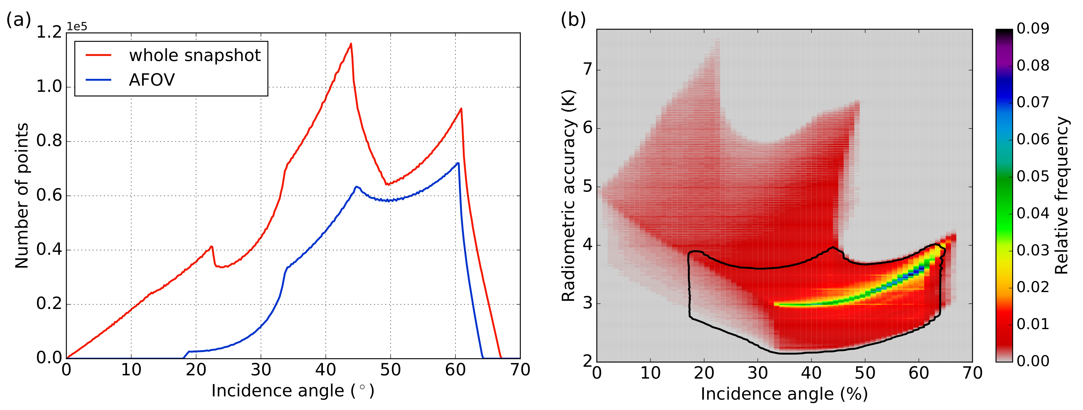
For the present analysis, we assume that the largest source of brightness temperature uncertainties are the radiometric accuracies of the measurements within a snapshot and neglect other uncertainties related to RFI, atmospheric impacts and cosmic and galactic radiation. Thus, the synthetic dataset should well represent the SMOS characteristics in terms of the incidence angle distribution and the radiometric accuracies. A typical frequency distribution of incidence angles for one day north of 50 N is shown in Figure 1a. To construct the test dataset, incidence angles are randomly drawn from this distribution. To get a reasonable representation of the entire frequency distribution a total number of about 100,000 angles is necessary. A two-dimensional frequency distribution showing incidence angles and their corresponding radiometric accuracies are presented in Figure 1b.
The synthetic dataset is constructed by applying the following steps: first, n random incidence angles are drawn from the incidence angle distribution in Figure 1a with a precision of 0.01. Here, n represents the number of SMOS measurements at a certain grid point. These incidence angles are then used to calculate polarized brightness temperatures based on the Fresnel equations over sea ice and ocean surfaces (see below). Finally, a radiometric accuracy value is assigned to each incidence angle and added to the brightness temperature value. For this purpose, radiometric accuracy distributions are calculated for each 1 incidence angle bin of the distribution shown in Figure 1b and a value is randomly drawn from this distribution with a precision of 0.01 K.
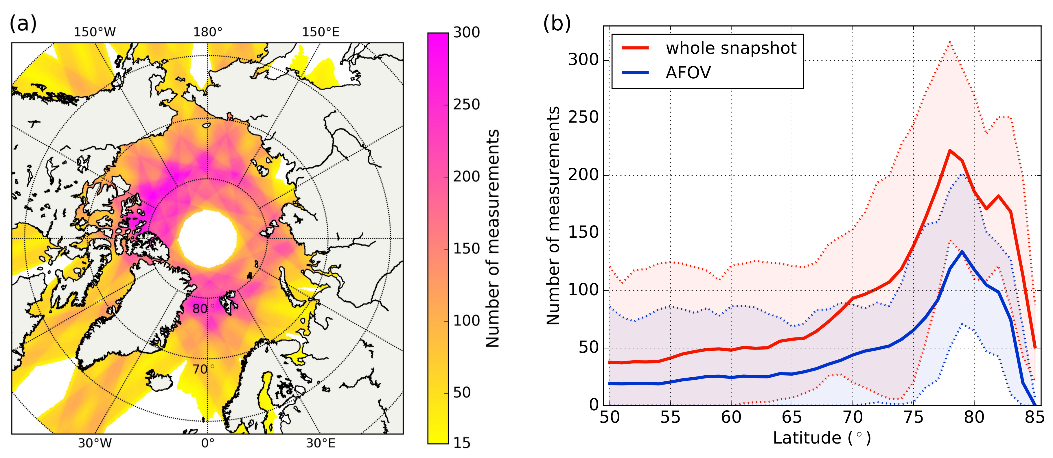
The typical number of measurements during one day using data from whole snapshots and from the alias-free field-of-view (AFOV) are presented in Figure 2. At 50 N, the number of measurements per day is quite variable with values between 0 and 100. A complete daily coverage is reached for the area north of 60 N for data from whole snapshots and north of 70 N for AFOV. The maximum of about 300 measurements for whole snapshots and 200 measurements for AFOV per day is located at about 78 N. To represent this large range of number of measurements per day, n is varied from to ( for AFOV). To assure that the whole incidence angle distribution is considered, calculations are repeated times for each n.
Brightness temperatures are calculated using the Fresnel equations for a specular plain surface e.g., [25]:
where and are the temperature and the permittivity of the surface, and are the reflection coefficients for vertical and horizontal polarizations. We neglect the impact of surface roughness and different layers within the sea ice and calculate the reflection coefficients as:
We consider two different surfaces: sea ice with a surface temperature of C and sea water with C. For simplicity, we consider multi-year sea ice with a low brine fraction (brine volume approx. 0.008) for which we obtain a permittivity of at a frequency of 1.4 GHz using an empirical formulation by Vant et al. [26]. The complex permittivity of sea water is calculated using an empirical formula by Klein and Swift [27] assuming a salinity of , which gives .
2.2.2. Fitting Methods
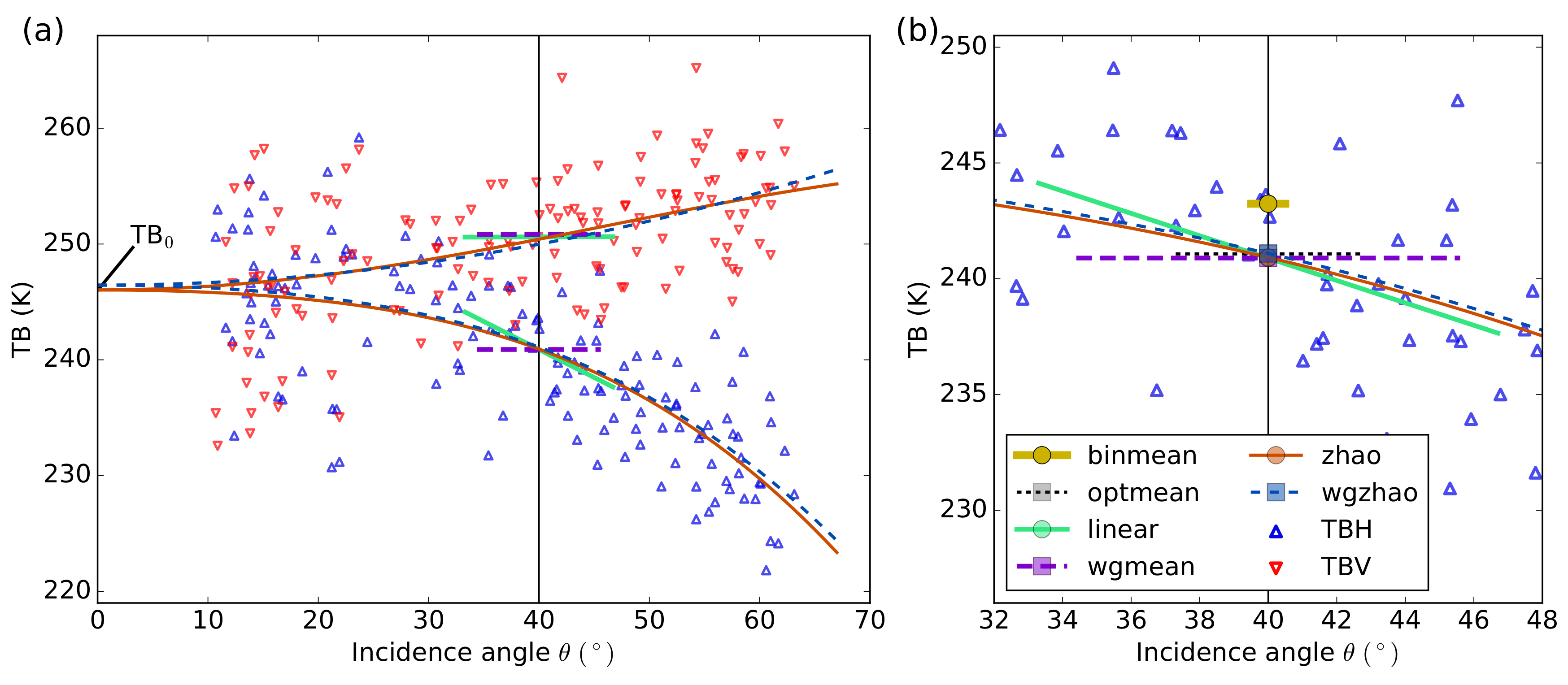
We compare six fitting methods of different complexities, ranging from simple (weighted) bin means, to linear and more complex regressions. The methods are described in the following and illustrated in Figure 3. An overview of the methods is given in Table 1.
- 1-bin mean (binmean):The simplest method is a binning of the brightness temperature values into incidence angle bins with a fixed width of . Here, we consider a bin width of .
- Bin mean with optimized interval (optmean):Instead of using a fixed bin width as in method 1, we consider a bin mean with an optimized bin width . The determination procedure of is described in Section 2.2.3.
- Weighted mean with optimized interval (wgmean):The different radiometric accuracy values (RA) of each measurement are used to calculate a weighted mean. As for method 2, an optimal interval width is determined for this procedure (Section 2.2.3).
- Linear fit with optimized interval (linear):and as functions of incidence angle are piecewise approximated by straight lines. We determine an optimal incidence angle interval within which data are considered for the linear fit (Section 2.2.3).
- Simple two-step fit based on Zhao et al. [12] (simplezhao):We also use a fitting function based on a formulation developed by Zhao et al. [12] to refine the characteristics of multi-angular SMOS observations. It consists of a two-step regression approach. As a first step, the brightness temperature at nadir ()—which is the same for H and V polarizations—is estimated from the brightness temperature intensity. In the original approach by Zhao et al. [12], was estimated from a quadratic fit to the brightness temperature intensities. We simplified this first step and calculate as the average of all brightness temperature intensity values with incidence angles below 40. Below 40, the change of the TB intensity with incidence angle is negligible [3]. is then used as a control point in the second step of the regression, where two separate functions are used for and :with . The fit is performed using a least-square method.
- Weighted Zhao fit (wgzhao):Zhao et al. [12] implemented the two-step regression approach described in method 5 by introducing additional weights based on the radiometric accuracy (RA) of the TB measurements. This means that, rather than minimizing as in method 5, the term is minimized.
2.2.3. Optimal Interval
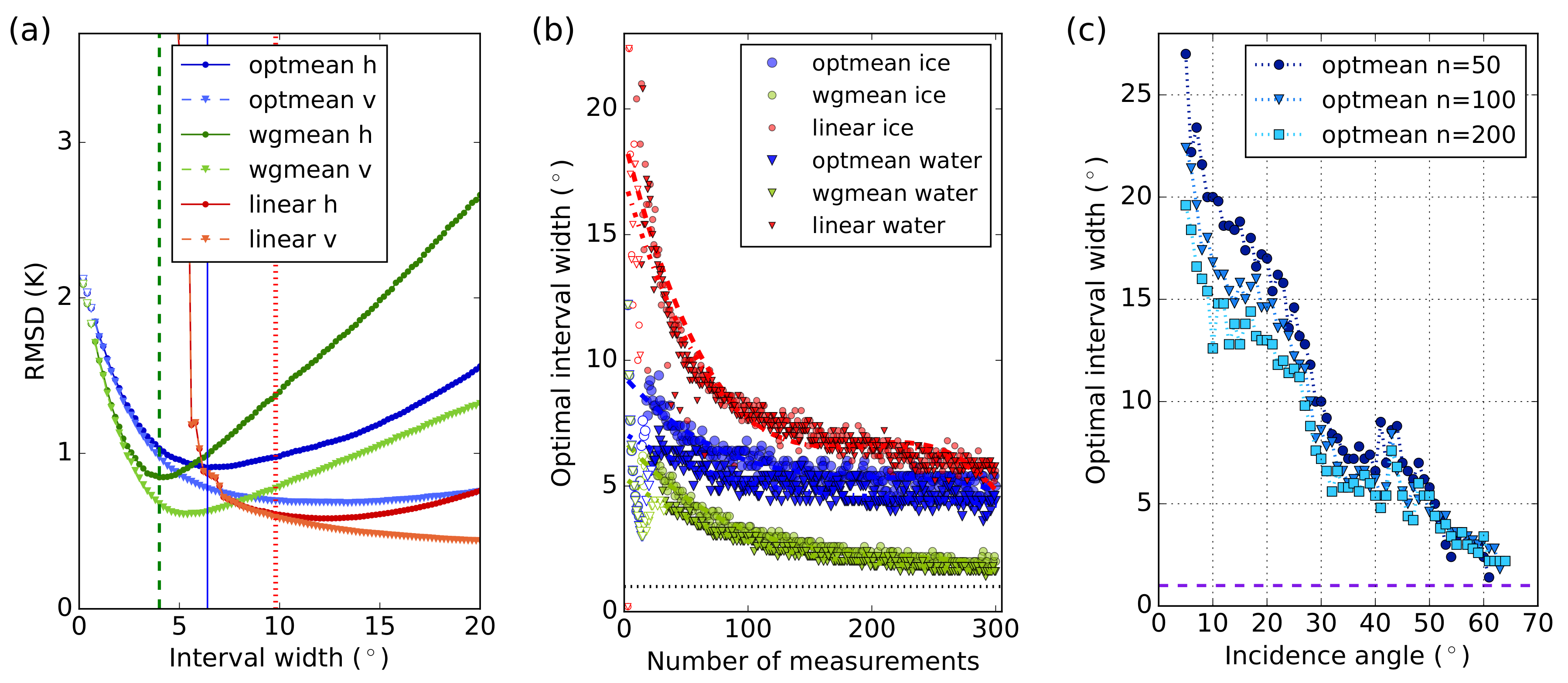
To determine the optimal interval widths for methods 2, 3, and 4, is varied from 0.2 to 28 in steps of 0.2. For each considered number of incidence angles n, the procedure is repeated times and a root mean squared difference to the original testing data is calculated as
For , the RMSD as a function of is exemplarily shown in Figure 4a. It is evident that most curves show a distinct minimum or level off for a certain interval width. Thus, it is possible to determine an optimal interval width . We discard those values, for which the amount of missing data—i.e., the number of times when the method did not yield any value—exceeds 30% (empty symbols in the figure). For each method, is then determined as the minimum (or the point where the curve levels off) of the curve (H or V polarization) with the overall higher RMSD. differs for different methods and also for different numbers of measurement pairs n (see Figure 4b) but shows only small differences between sea ice and water surfaces. The largest optimal intervals are found for the linear method and the smallest ones for wgmean. For all further analyses, a third-degree polynomial is fitted through the curves in Figure 4b, considering only values for which the amount of missing values is smaller than 2%.
The optimal interval also differs for different incidence angles (Figure 4c). For the optmean method, it is larger than for incidence angles near nadir and decreases to about 2 or 3 for . This already indicates that a constant averaging interval—especially when it is as small as 1 as in method 1—might not yield the most accurate fitting results.
2.2.4. Results for Different Fitting Methods
To compare the different methods, we calculated the RMSD (Equation (4)) between the fitted and the modeled brightness temperatures for different numbers of measurements n and different incidence angles. Exemplary results for a sea ice surface and the SMAP incidence angle are presented in Figure 5. For simplicity, the RMSD values shown are combined ones for TBV and TBH. It is evident that the smallest RMSD values occur for the two methods based on the Zhao fit (simplezhao and wgzhao). Even when only a few measurements are available (), the fit yields a high accuracy with RMSD values below 1 K. In addition, the number of missing values decreases to values below 1% for .
When more measurements are available (), the linear, optmean and wgmean methods also yield small RMSD values comparable to those from the simplezhao and wgzhao methods. The 1-bin mean has the largest RMSD values and the largest amount of missing data and is thus the least suitable fitting method when daily values in the polar regions are considered.
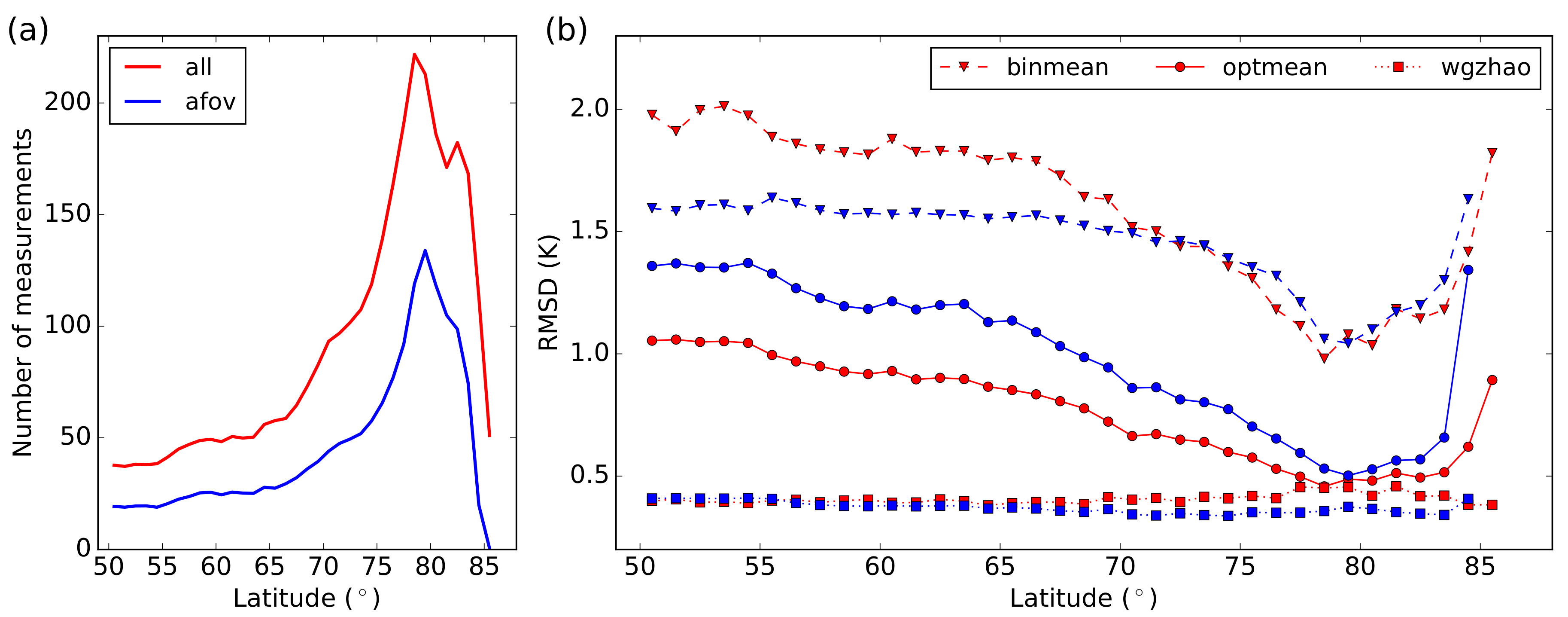
Qualitatively, the results are very similar for a water surface and for other incidence angles in the range of 29 to 60 (not shown). Larger differences occur when only data from the alias-free-field-of-view are considered instead of data from whole snapshots. For the same number of measurements, fits using AFOV data have RMSD values that are about 0.1 to 0.3 K smaller than those from whole snapshots (not shown). However, for the same latitude, less measurements are available for AFOV, which has to be accounted for when evaluating the methods. Thus, the RMSD values as a function of latitude are shown in Figure 6. It is evident that using AFOV data instead of data from whole snapshots only yields smaller RMSD values for the binmean method equatorward of 70. For all other methods, using AFOV does not decrease the RMSD notably or even causes an increase. These results are robust for sea ice and water surfaces and for the considered incidence angle range of 29 to 60 (not shown).
2.2.5. Computing Performance
Besides the accuracy of the fit, the required computing time is also of interest when choosing a fitting method, e.g., for a near-real time operational production of daily sea ice thickness maps average run times should be much smaller than 12 h. With roughly 200,000 grid points north of 50 N in the SMOS L1C sea product, this results in a maximum computing time of no more than 200 ms.
Average computing times of the considered methods are presented in Table 2. The absolute numbers obviously depend on the used software and hardware (The computations were performed on a 8xQuad-Core AMD Opteron 8356 processor with 2.3 GHz. The fitting functions were implemented in Python and optimized for speed using Cython.) and are only presented here for a relative intercomparison of the different methods.
The two methods based on the Zhao fit require more than 100 times more computing time than those methods based on a simple averaging. Nevertheless, the overall computing time for a daily polar product is on the order of 3 h and is thus acceptable for operational use.
2.2.6. Final Choice of Optimal Fitting Method
From the six evaluated fitting methods, the two Zhao fits show the overall best performance. They yield a high accuracy and only a few cases with missing data even for a small number of measurements. These advantages justify the relatively large computing times. The Zhao methods are also beneficial when more than one specific incidence angle is considered since any incidence angle can be reproduced from the same set of six fitting parameters.
In cases when the available number of measurements is much larger than 50, the method with an optimized averaging interval is also an accurate and fast method. Such large n are found, for example, between 70 and 83 N/S or when data from several days is considered. For this method, it is necessary to adjust the optimal averaging interval according to the incidence angle with values increasing from for to for incidence angles close to nadir. Consequently, an averaging interval of only 1 as in the binmean method is too small.
We limited this analysis to pure statistical and semi-empirical methods. It should be noted here that there are also fitting methods based on the Fresnel functions representing the physical processes of the scattering. One example is a two-layer Fresnel fit presented in Huntemann [11], which considers a snow layer on top of a sea ice layer. Such a complex fitting function results in computing times in the order of 1 s (not shown), which is too large for operational purposes. In addition, physical fit functions require a priori knowledge or assumptions about the surface characteristics, such as the surface roughness or the presence of a snow layer on top of the ice.
On these grounds, we decided to use the weighted Zhao fit for the comparisons of brightness temperatures from SMOS and SMAP presented in the next section. We exclude cases with very few data points and only perform the fit for .
2.3. Sea Ice Thickness Retrieval Algorithm
In the next step, brightness temperature intensities are used to calculate sea ice thickness. The sea ice thickness retrieval is based on the algorithm presented in Tian-Kunze et al. [3], which consists of a combination of a thermodynamic model with a sea ice radiation model. Here, we only briefly summarize the retrieval algorithm and refer to the original publication for more details.
The one-dimensional thermodynamic model is used to calculate sea ice temperature and salinity. It considers one sea ice layer covered by a snow layer and uses 2 m-air temperature and 10 m-wind speed from the Japanese 55-year reanalysis (JRA) as input data, as well as a weekly climatology of sea surface salinity. The radiation model consists of a single plane sea ice layer and calculates brightness temperatures based on the dielectric properties of sea ice. In a second step, the effect of the sub-pixel thickness heterogeneity is addressed by assuming a log-normal distribution of the sea ice thickness. In the following, we refer to these two different retrieval steps as the “plane layer” and the “heterogeneous” ice thicknesses.
In Tian-Kunze et al. [3], the retrieval algorithm was implemented as an iterative method. A first guess of the ice thickness is obtained from an empirical function [2] and a corresponding brightness temperature is calculated using the thermodynamic and the radiation model. They compare the calculated TB to the measured one and adjust the estimated sea ice thickness accordingly using a linear approximation method. This process is repeated until the TB difference is smaller than 0.1 K or the change in sea ice thickness is smaller than 1 cm. To decrease the computing time, the results are stored as a lookup table for given air temperatures, wind speeds, and sea water salinities.
Here, we use a direct approach instead, which does not require an arbitrarily chosen convergence criterion but otherwise yields the same results. For every combination of given air temperature, wind speed, and sea water salinity, we calculate TBs for a range of sea ice thicknesses from 0 to 4 m in steps of 1 cm. As for the iterative method, the obtained TBs as a function of ice thickness are stored in a lookup table. In the retrieval, we determine for every TB pixel those values of air temperature, wind speed, and water salinity in the lookup table that are closest to the pixel values of temperature and wind speed from JRA and of water salinity from the weekly climatology and extract the corresponding TBs as function of ice thickness. The measured TB is then used to interpolate an ice thickness value from this relationship.
At L-band frequencies, the radiation penetrates sea ice up to a certain depth only, depending on sea ice temperature and salinity. When the sea ice is thicker than the penetration depth, it is not any more possible to obtain a thickness information. We refer to this situation as "saturation" and exclude saturated plane layer ice thicknesses from the comparison of thicknesses derived from SMOS and SMAP TBs in Section 3.3.
3. Results
In this section, we present a comparison of daily mean fields of measured brightness temperatures and derived sea ice thicknesses from SMOS and SMAP in both hemispheres. As a first step, we demonstrate the impact of different fitting methods on the day-to-day TB variability over a stable target, such as an ice shelf (Section 3.1). In Section 3.2, we present a detailed comparison of TBs from SMOS and SMAP over the polar ocean regions. We evaluate differences over different surface types, such as seasonal and multi-year sea ice cover and ocean (see boxes in Figure 7), as well as over the whole Arctic and Antarctic ocean regions. In Section 3.3, we then compare sea ice thicknesses derived from the SMOS and SMAP brightness temperatures.
3.1. Brightness Temperature Comparison over a Stable Target Using Different Fitting Methods
Due to the large penetration depth of L-band radiation in freshwater ice, the day-to-day TB variability over an ice shelf can be assumed to be very small. This makes ice shelves an ideal target to test the impact of different fitting methods on the TB values. To assure the best temporal stability, we choose pixels in the center of the two large Ronne and Ross ice shelves (indicated by dots in Figure 7). For the comparison, we use TBs from a 30-day period with negligible temporal trends.
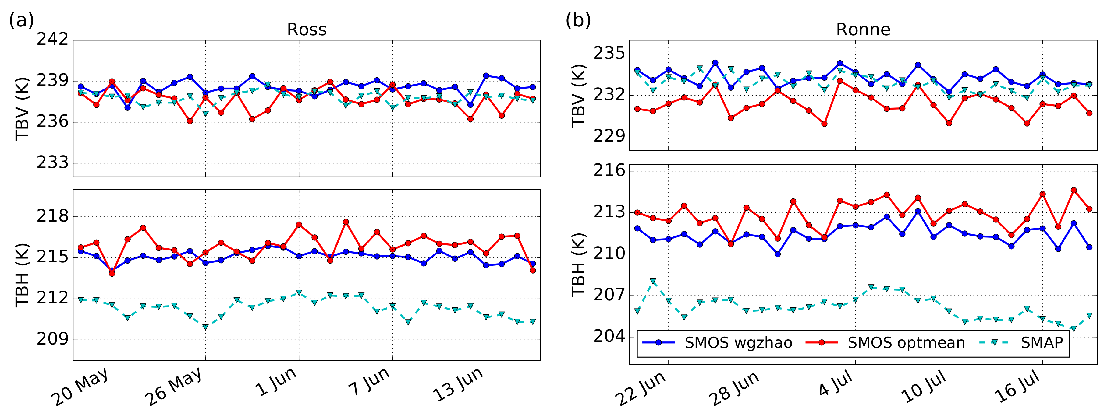
Here, we only compare the results from the optimal fitting method found in Section 2.2.6—the weighted Zhao fit (wgzhao) with one of the simpler and faster methods—a bin mean with an optimized interval of 5 (optmean). Time series of polarized TBs from SMOS using the two different fit methods over the two targets are shown in Figure 8. SMAP TBs are added for comparison. Temporal averages and standard deviations of the time series are summarized in Table 3.
It is evident that the optmean method generally produces a higher standard deviation (0.8–1.0 K) of the daily TB values than the wgzhao method (0.4–0.7 K) at both locations. Additionally, the choice of fitting method also impacts the mean TB values by about 1–2 K. For SMAP, standard deviations are comparable to those of the wgzhao method (0.4–0.8 K). However, the mean values for horizontally polarized TBs from SMAP show a bias of about 5–6 K with respect to SMOS TBs.
3.2. SMAP and SMOS Brightness Temperature Comparison
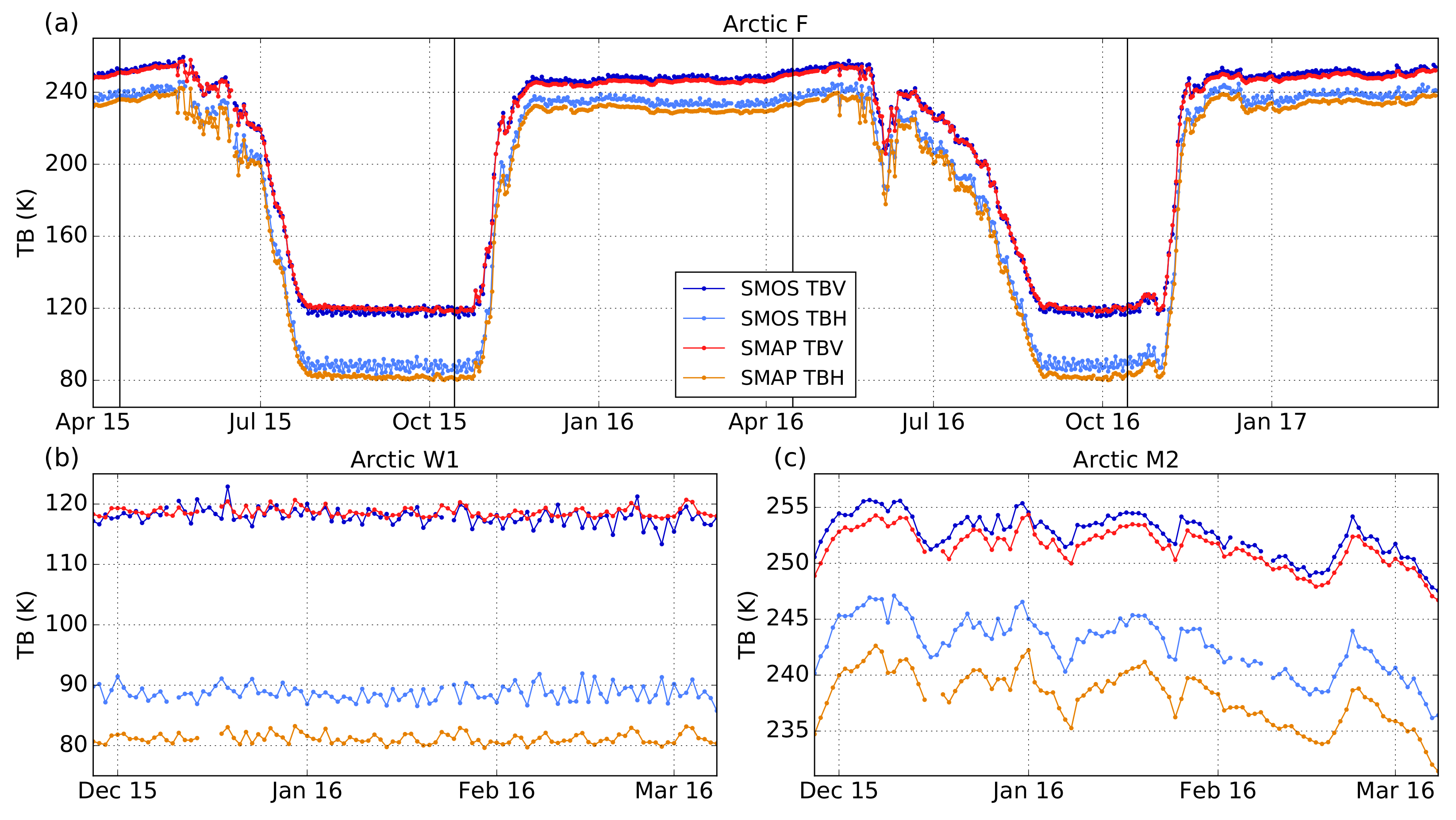
In this section, we compare TBs from SMOS and SMAP over the Arctic and Antarctic ocean regions poleward of 50 N/S. Different surface types–such as first-year ice, multi-year ice, and open ocean—are considered separately. To reduce the impact of different sensor footprints and gridding artifacts, TBs are averaged over boxes of 200 km times 200 km. The considered areas are marked as boxes in Figure 7 and exemplary timeseries of daily TB values are shown in Figure 9. Statistical values of the differences of SMOS and SMAP TBs for all boxes for the 2-year time period from 1 April 2015 to 31 March 2017 are presented in Table 4.
The overall TB variability from SMOS and SMAP over sea ice surfaces agrees very well with correlation coefficients of 0.99 or above. Correlations remain very high when only thicker ice during the freeze-up period is considered (0.94–0.98, see Table 4). However, TBs show a bias which is especially pronounced for horizontal polarization. TBs from SMAP over sea ice are on average 4–5 K lower than those from SMOS. The bias is even larger over water with values in the order of 6–7 K. Overall, the polarization difference (TB-TB) for SMAP is about 7 K larger over water and about 2.5 K larger over thick ice than for SMOS.
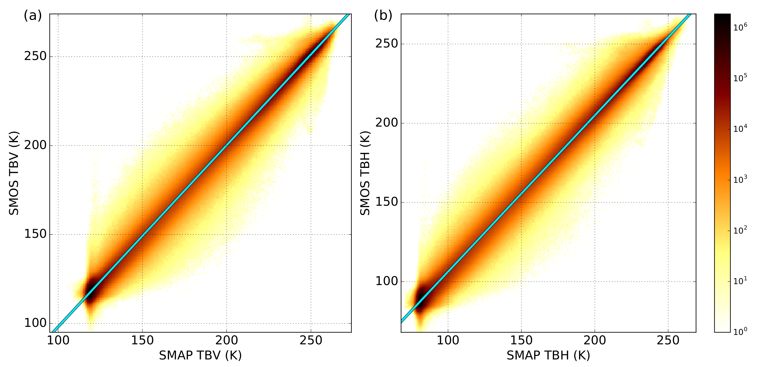
The TB differences between SMOS and SMAP over the polar ocean regions can be represented by a straight line (Figure 10). A similar approach has been suggested by Huntemann et al. [15]. We found that the respective regression coefficients show only very small temporal variability and differences between the two hemispheres are negligible (not shown). Thus, we calculate the following constant regression lines:
These regression coefficients can be used to adjust the TB bias and to calibrate the measurements from the two sensors to each other. Since without further comparison to other TB datasets from in situ campaigns or from validated models it is difficult to determine which one of the two sensors is closer to the truth, we arbitrarily decided to calibrate SMAP TBs to those from SMOS. This also makes sense for practical reasons since the SMOS timeseries extends longer into the past.
After bias adjustment, the root mean squared differences between SMOS and SMAP TBs over ice decrease especially for horizontal polarization from about 5 K to 1–3 K (Table 4). RMSDs over thick ice after adjustment are in the order of 1 K for both polarizations and are thus within the range of typical uncertainties of the daily TB products from both sensors.
Even though results over ice are generally very similar over both hemispheres, there are notable differences over water surfaces. In particular, the water box W2 in the Arctic shows much lower correlations than the two Antarctic water boxes. In box W2, RMSDs also remain large with values of 6–7 K after bias adjustment, while they decrease to values of 1–2 K in the Antarctic (and over box W1 in the Arctic). This effect is probably due to the impact of RFI on SMOS TBs, which is pronounced in many Arctic regions but mostly not present in the Antarctic. The data loss due to RFI causes an increase of noise in the SMOS TB signal and thus increases the day-to-day variability (see Figure 9).
3.3. Sea Ice Thickness
In this section, we compare sea ice thickness (SIT) retrieved from SMOS and SMAP brightness temperature intensities at an incidence angle of 40. We apply the retrieval algorithm described in Section 2.3 to produce daily SIT fields for one winter season (15 October 2015 to 15 April 2016) in the Arctic. We start by comparing SMOS and SMAP sea ice thicknesses (Section 3.3.1) to address the following questions: How do the TB differences and biases found in Section 3.2 translate to SIT differences? Which differences remain after TB bias adjustment? In addition, we evaluate the differences caused by changing the retrieval algorithm from near-nadir to an incidence angle of 40 (Section 3.3.2). Finally, we discuss the potential of a combined SIT product from SMOS and SMAP (Section 3.3.3).
3.3.1. SMOS and SMAP Sea Ice Thickness Comparison
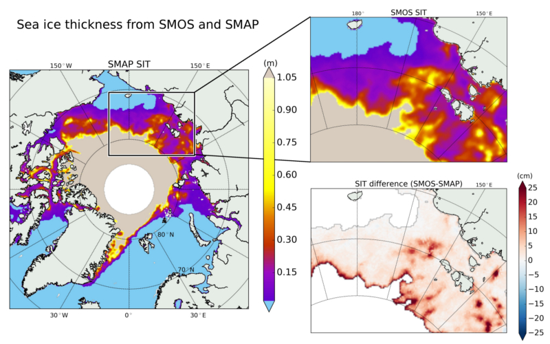
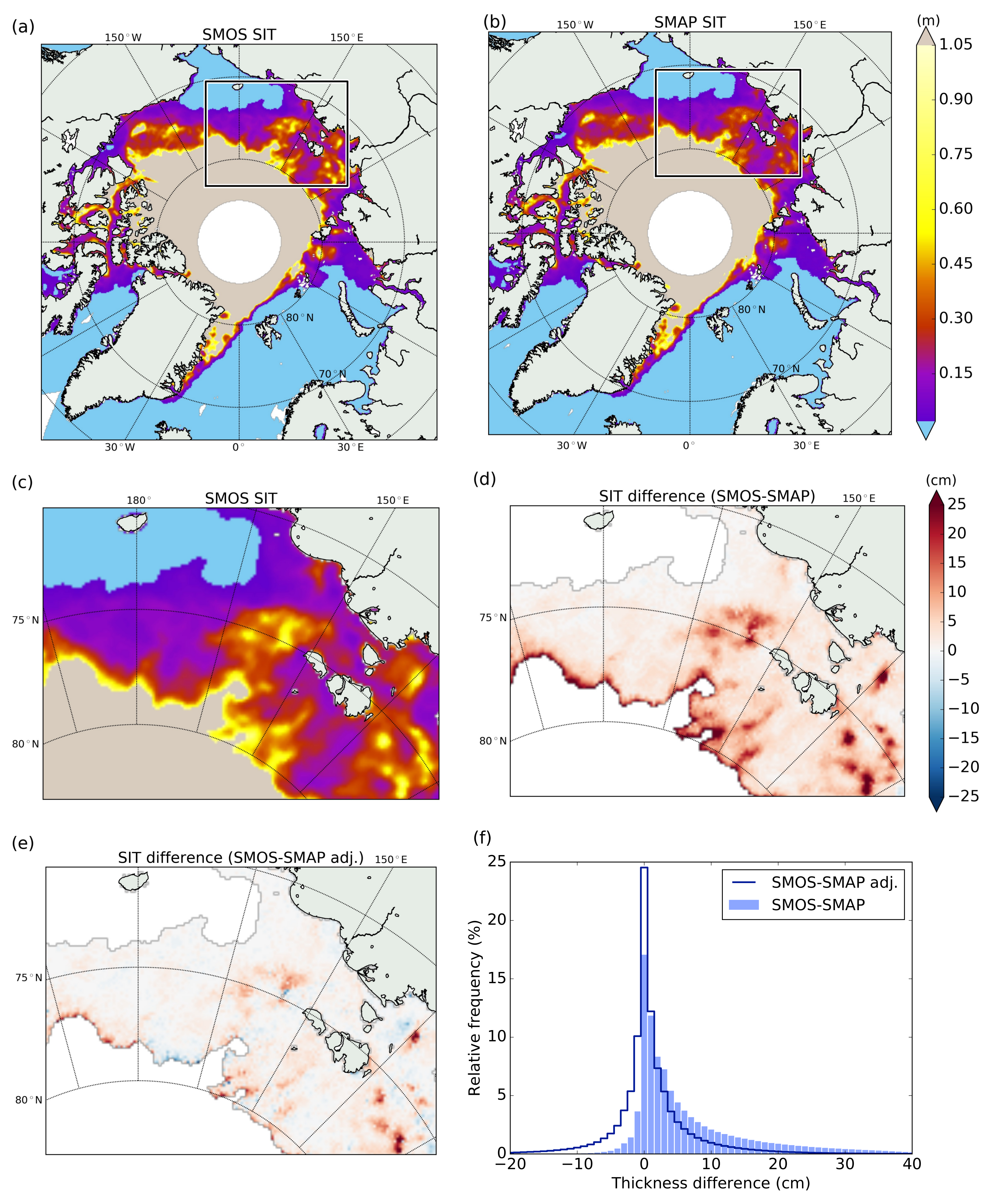
Exemplary maps of SIT from SMOS and from SMAP are presented in Figure 11. For the comparison, we exclude regions with a saturation ratio of 100% (gray areas) or with an ice thickness below 2 cm (blue areas) in any of the two products. It is evident from the SIT difference map in Figure 11 that the TB intensity bias of about 2–3 K also causes an SIT bias, where SMOS generally produces larger ice thicknesses than SMAP. Averaged over the whole winter season, SMOS thicknesses are on average about 7 cm larger than SMAP thicknesses. The RMSD is 12 cm.
When the TB bias is adjusted before the retrieval, the bias reduces to only about 1 cm, which is approximately the desired accuracy for the retrieval. The RMSD is still as large as 7 cm after the bias adjustment. This is probably related to the different overpass times of the two sensors. Especially in regions with frequent lead openings–which can refreeze within hours–the average ice thickness within a sensor footprint can change by a few centimeters within a day.
3.3.2. Incidence Angle Dependency
The retrieval algorithm by Tian-Kunze et al. [3] was originally developed for brightness temperature intensities averaged over the near-nadir incidence angle range from 0 to 40. In this section, we evaluate the changes occurring when the retrieval is adapted to the SMAP incidence angle of 40.
Considering only ice thicknesses from 2 cm up to the saturation thickness and averaging over the winter season from 15 October 2015 to 15 April 2016, we find that sea ice thicknesses are on average 2.3 cm larger when is used. The overall RMSD is about 6 cm. Even though this bias is small, it indicates that the incidence angle dependency is not represented perfectly in the retrieval model. One possible reason might be the lack of a snow layer in the radiation model. Even though snow on sea ice mostly affects the sea ice temperature, a study by Maa et al. [10] indicated that there is also a smaller radiative impact that changes with incidence angle.
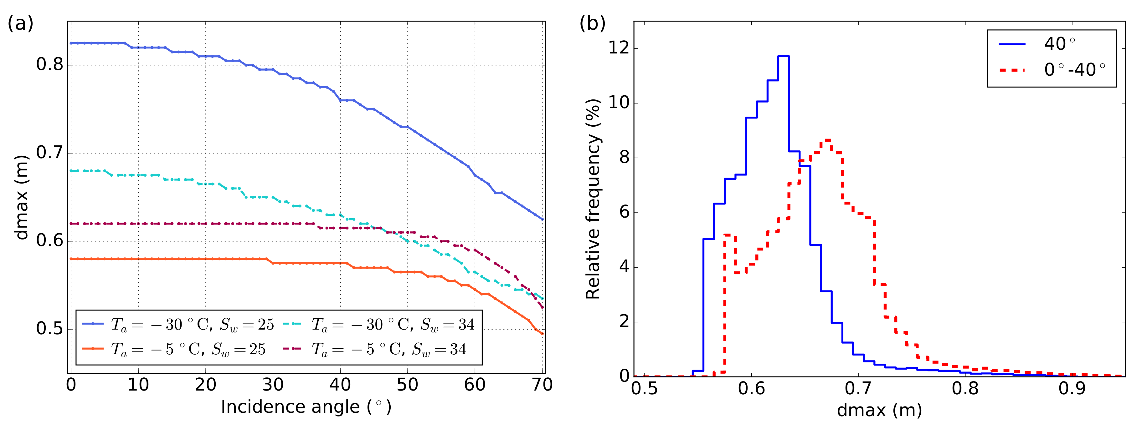
The choice of incidence angle also affects the penetration depth of L-band radiation and thus the saturation thickness. Figure 12 shows theoretical curves of as a function of incidence angle for idealized cases. While differences are small for relatively warm and salty ice, can be up to 8% larger for than for in cold, low-salinity conditions. The changes of saturation thickness are also evident in the histograms of for all considered cases during the winter season 2015/2016 (Figure 12). Average saturation thicknesses decrease from 66 cm near-nadir to 62 cm for . Consequently, there is also an increase of the number of saturated pixels of about 10%.
3.3.3. A Combined Sea Ice Thickness Product from SMOS and SMAP
We have demonstrated that, with proper fitting procedures and bias adjustments, it is possible to combine SMOS and SMAP brightness temperature measurements. The main advantage of the merged product is the decreased data loss. This becomes evident when looking at the median data loss north of 50 N averaged over the winter season 2015/16. We find the largest value of 11.9% for SMOS, where a substantial amount of data is contaminated by RFI. There is also some data lost at the swath edges, where not enough measurements are available for the fitting procedure. SMAP shows a smaller data loss of 3.5% and in the combined product the data loss decreases to only 0.9%.
With their differences in equator crossing times of 12 h, the two datasets also nicely complement each other and thus ensure a better daily data coverage equatorward of 70. For sea ice applications, this is especially relevant in the Antarctic, where a substantial part of the sea ice area extends to lower latitudes (see Figure 7). In addition, a combination of two sensors will also ensure the continuation of the time series, if one of the sensors stops delivering data in the future.
In this light, we find it beneficial to change the SMOS sea ice thickness retrieval from the near-nadir incidence angle range (0–40, Tian-Kunze et al. [3]) to the SMAP incidence angle of 40. Even though the penetration depth slightly decreases for larger incidence angles (Section 3.3.2), this is outweighed by the better data coverage.
4. Discussion
To obtain brightness temperatures at a specific incidence angle from the multi-angular SMOS measurements, we evaluated the performance of six different fitting methods based on their accuracy and computing time. Even though the bin mean is the fastest method, it only yields accurate results if the averaging interval is optimized and if more than 50 measurements are available. The optimal interval decreases from about 20 near-nadir to about 3 at , indicating that a fixed interval width of 5 as in the CATDS dataset [8] is not an optimal choice. The Zhao fit including a weighting by the radiometric accuracy showed the overall best performance, even for a small number of 15 to 50 measurements. These results are in line with those by Zhao et al. [12] who found that the fitted TBs over land areas are more consistent with results from a radiative transfer model than the CATDS data.
We compared two years of daily polarized brightness temperatures from SMOS and SMAP over the sea-ice-covered polar oceans and found a good overall agreement. However, we found a cold bias of SMAP compared to SMOS TBs of 1.4 K for vertical and about 4 K for horizontal polarizations over sea ice. Over water, the bias for horizontal polarization even exceeds 6 K. These numbers result in a bias of the TB intensity of about 2.7 K for both ice and ocean surfaces. In the following, we discuss different possible reasons for the TB bias, which have been partly suggested in the literature.
Differences in corrections for galactic and atmospheric effects were found to cause TB biases between SMAP and Aquarius over land and over the Antarctic continent [29]. However, since we compared uncorrected TOA brightness temperatures for both SMOS and SMAP, we can certainly exclude this reason. We can also exclude RFI contamination of SMOS data as a main reason for the bias. RFI is not an issue around Antarctica, but we found biases there as well, which are consistent with values over the northern polar oceans. Orbital differences could also play a role since SMOS and SMAP have different equator crossing times at 6:00 and 18:00, respectively. However, this would result in bias values and signs changing with time and region, which is not the case as our analysis has shown.
Even though we did not find large differences of the biases observed in different regions over Arctic and Antarctic sea ice and ocean regions, results might be different in lower latitude regions. Other studies with co-located SMOS and SMAP overpasses showed a negligible bias of about 0.5 K over oceans far from the coast, but a larger bias of about 2.7 K over land for both horizontal and vertical polarizations [13,30]. This land bias is very similar to the TB intensity bias of about 2.7 K we found over multi-year ice. An initial analysis by Peng et al. [31] of a re-calibrated version of the SMAP brightness temperatures—which is planned to be released in 2018—showed a reduced bias over land. Thus, this bias is probably related to the calibration of the SMAP data.
This does not explain the different findings over ocean in Bindlish et al. [13] and in this study, however. A possible reason for this bias is the so-called land-sea contamination (LSC), which is a known issue for SMOS brightness temperatures. Though the exact reasons for LSC are still under discussion [32], it is known that large TB contrast between land (or ice) and ocean surfaces result in artificially increased TBs over the oceans in coastal regions. This bias can exceed 3 K for TB intensity in the polar regions [33], which is in line with our TB intensity biases over oceans of about 2.5–3.0 K.
5. Conclusions
We presented a comparison of brightness temperatures and derived sea ice thicknesses from SMOS and SMAP over the polar ocean regions. As a first step, the multi-angular SMOS measurements were fitted to the SMAP incidence angle of 40. For this purpose, we tested different fitting methods, such as a bin mean or a linear fit with fixed or optimized bin widths and a more sophisticated fitting function using a two-step regression method by Zhao et al. [12]. To evaluate the accuracy of the different fitting methods, we constructed a synthetical dataset based on SMOS characteristics in terms of incidence angle distribution and radiometric accuracies in high latitudes. We found that the weighted Zhao fit performs best, yielding a high accuracy even for a small number of measurements of only 15. We could also demonstrate this good performance of the weighted Zhao fit over a stable target. TB time series over the Ross and Ronne ice shelves showed a smaller day-to-day variability for the weighted Zhao fit compared to the bin mean method.
Daily values of fitted SMOS TBs were then compared to those from SMAP over the polar oceans, over thin first-year-ice, and over thicker multi-year-ice. Generally, the time series agreed very well, with correlations over sea ice exceeding 0.99. However, we found a cold bias of SMAP compared to SMOS TBs of 2.7 K for TB intensity over both ice and ocean surfaces. This bias is even larger for horizontal polarization, with about 4 K over sea ice and more than 6 K over water. Since this bias is mostly constant in time and space, it can be adjusted using a linear fitting function.
The TB intensity bias also translates to a sea ice thickness bias. Averaged over one winter season, SMOS thicknesses are 7 cm larger than SMAP thicknesses with an RMSD of 12 cm. After adjustment of the TB bias, the RMSD values for brightness temperature over thick ice decrease to about 1 K, which is within the sensor accuracies.
We also evaluated the changes caused by adapting the SMOS retrieval algorithm from near-nadir incidence angles [3] to the SMAP incidence angle of 40. Since the penetration depth of L-band radiation in sea ice decreases with increasing incidence angle, the maximum retrievable thickness is on average 4 cm smaller at 40 than for the near-nadir retrieval. This results in an increase of the number of saturated pixels of about 10%.
We conclude that it is feasible to combine SMOS and SMAP brightness temperatures for an improved retrieval of sea ice thickness. The overall data loss—mostly due to RFI contamination of SMOS measurements—can be largely reduced. In addition, the region of daily coverage is extended equatorwards resulting in a better coverage of the sea ice covered areas around Antarctica. Most importantly, a combined dataset from the two sensors ensures a consistent continuation of the L-band sea ice thickness timeseries in the future even if one of the sensors stops delivering data. This improved data coverage and availability outweighs in our opinion the slight increase of saturated pixels caused by the adaption of the retrieval algorithm from near-nadir incidence angles to the SMAP incidence angle.
With two sensors in orbit and multiple overpasses per day in high latitudes, it is now also possible to look at short-time-changes of the sea ice thickness in a specific region. Such a swath based analysis opens up new possibilities for case studies or for assimilation of L-band sea ice thickness data into forecast models.
Acknowledgments
This work was supported by the project SPICES (space-borne observations for detecting and forecasting sea ice cover extremes) funded by the European Union’s Horizon 2020 Programme (grant agreement No. 640161). L.K. was funded by Deutsche Forschungsgemeintschaft (DFG EXC177). We thank Xiangshan Tian-Kunze for pre-processing the SMOS L1C data and Valentin Ludwig for his preparatory work concerning the different fitting methods. We also thank the three anonymous reviewers for their valuable comments.
Author Contributions
A.S. and L.K. jointly contributed to the concept of this paper. A.S. analyzed the data and wrote the manuscript.
Conflicts of Interest
The authors declare no conflict of interest. The founding sponsors had no role in the design of the study; in the collection, analyses, or interpretation of data; in the writing of the manuscript, and in the decision to publish the results.
Abbreviations
The following abbreviations are used in this manuscript:
| AFOV | Alias-free field-of-view |
| RFI | Radio frequency interference |
| RMSD | Root mean squared differences |
| SIT | Sea ice thickness |
| SMAP | Soil Moisture Active Passive |
| SMOS | Soil Moisture and Ocean Salinity |
| TB | Brightness temperature |
| TOA | Top of atmosphere |
References
- Richter, F.; Drusch, M.; Kaleschke, L.; Maaß, N.; Tian-Kunze, X.; Mecklenburg, S. Arctic sea ice signatures: L-band brightness temperature sensitivity comparison using two radiation transfer models. Cryosphere 2018, 12, 921–933. [Google Scholar] [CrossRef]
- Kaleschke, L.; Tian-Kunze, X.; Maaß, N.; Mäkynen, M.; Drusch, M. Sea ice thickness retrieval from SMOS brightness temperatures during the Arctic freeze-up period. Geophys. Res. Lett. 2012, 39, 5501. [Google Scholar] [CrossRef]
- Tian-Kunze, X.; Kaleschke, L.; Maaß, N.; Mäkynen, M.; Serra, N.; Drusch, M.; Krumpen, T. SMOS-derived thin sea ice thickness: algorithm baseline, product specifications and initial verification. Cryosphere 2014, 8, 997–1018. [Google Scholar] [CrossRef] [Green Version]
- Huntemann, M.; Heygster, G.; Kaleschke, L.; Krumpen, T.; Mäkynen, M.; Drusch, M. Empirical sea ice thickness retrieval during the freeze-up period from SMOS high incident angle observations. Cryosphere 2014, 8, 439–451. [Google Scholar] [CrossRef] [Green Version]
- Kaleschke, L.; Tian-Kunze, X.; Maaß, N.; Beitsch, A.; Wernecke, A.; Miernecki, M.; Müller, G.; Fock, B.H.; Gierisch, A.; Schlünzen, K.H.; et al. SMOS sea ice product: Operational application and validation in the Barents Sea marginal ice zone. Remote Sens. Environ. 2016, 180, 264–273. [Google Scholar] [CrossRef] [Green Version]
- Ricker, R.; Hendricks, S.; Kaleschke, L.; Tian-Kunze, X.; King, J.; Haas, C. A weekly Arctic sea-ice thickness data record from merged CryoSat-2 and SMOS satellite data. Cryosphere 2017, 11, 1607–1623. [Google Scholar] [CrossRef]
- Le Vine, D.M.; Lagerloef, G.S.E.; Colomb, F.R.; Yueh, S.H.; Pellerano, F.A. Aquarius: an instrument to monitor sea surface salinity from space. IEEE Trans. Geosci. Remote Sens. 2007, 45, 2040–2050. [Google Scholar] [CrossRef]
- Al Bitar, A.; Mialon, A.; Kerr, Y.H.; Cabot, F.; Richaume, P.; Jacquette, E.; Quesney, A.; Mahmoodi, A.; Tarot, S.; Parrens, M.; et al. The global SMOS Level 3 daily soil moisture and brightness temperature maps. Earth Syst. Sci. Data 2017, 9, 293–315. [Google Scholar]
- De Lannoy, G.J.M.; Reichle, R.H.; Peng, J.; Kerr, Y.; Castro, R.; Kim, E.J.; Liu, Q. Converting Between SMOS and SMAP Level-1 Brightness Temperature Observations Over Nonfrozen Land. IEEE Geosci. Remote Sens. Lett. 2015, 12, 1908–1912. [Google Scholar] [CrossRef]
- Maaß, N.; Kaleschke, L.; Tian-Kunze, X.; Drusch, M. Snow thickness retrieval over thick Arctic sea ice using SMOS satellite data. Cryosphere 2013, 7, 1971–1989. [Google Scholar] [CrossRef]
- Huntemann, M. Thickness Retrieval and Emissivity Modeling of Thin Sea Ice at L-band for SMOS Satellite Observations. Ph.D. Thesis, University of Bremen, Bremen, Germany, 2015. [Google Scholar]
- Zhao, T.; Shi, J.; Bindlish, R.; Jackson, T.J.; Kerr, Y.H.; Cosh, M.H.; Cui, Q.; Li, Y.; Xiong, C.; Che, T. Refinement of SMOS Multiangular Brightness Temperature Toward Soil Moisture Retrieval and Its Analysis Over Reference Targets. IEEE J. Appl. Earth Obs. Rem. Sens. 2015, 8, 589–603. [Google Scholar] [CrossRef]
- Bindlish, R.; Jackson, T.J.; Chan, S.; Colliander, A.; Kerr, Y. Integration of SMAP and SMOS L-band observations. In Proceedings of the 2017 IEEE International Geoscience and Remote Sensing Symposium (IGARSS), Fort Worth, TX, USA, 23–28 July 2017; pp. 2546–2549. [Google Scholar]
- Al-Yaari, A.; Wigneron, J.P.; Kerr, Y.; Rodriguez-Fernandez, N.; O’Neill, P.; Jackson, T.; Lannoy, G.D.; Bitar, A.A.; Mialon, A.; Richaume, P.; et al. Evaluating soil moisture retrievals from ESA’s SMOS and NASA’s SMAP brightness temperature datasets. Remote Sens. Environ. 2017, 193, 257–273. [Google Scholar] [CrossRef]
- Huntemann, M.; Patilea, C.; Heygster, G. Thickness of thin sea ice retrieved from SMOS and SMAP. In Proceedings of the 2016 IEEE International Geoscience and Remote Sensing Symposium (IGARSS), Beijing, China, 10–15 July 2016; pp. 5248–5251. [Google Scholar]
- Mecklenburg, S.; Drusch, M.; Kerr, Y.H.; Font, J.; Martin-Neira, M.; Delwart, S.; Buenadicha, G.; Reul, N.; Daganzo-Eusebio, E.; Oliva, R.; et al. ESA’s soil moisture and ocean salinity mission: Mission performance and operations. IEEE Trans. Geosci. Remote Sens. 2012, 50, 1354–1366. [Google Scholar] [CrossRef] [Green Version]
- Zine, S.; Boutin, J.; Font, J.; Reul, N.; Waldteufel, P.; Gabarro, C.; Tenerelli, J.; Petitcolin, F.; Vergely, J.L.; Talone, M.; et al. Overview of the SMOS Sea Surface Salinity Prototype Processor. IEEE Trans. Geosci. Remote Sens. 2008, 46, 621–645. [Google Scholar] [CrossRef]
- SMOS L1C Processor. SMOS L1 Processor L1c Data Processing Model; Gutierrez, A., Castro, R., Vieira, P., Eds.; DEIMOS Engenharia: Lisboa, Portugal, 2014; Available online: https://earth.esa.int/documents/10174/1854456/SMOS_L1c-Data-Processing-Models (accessed on 5 March 2018).
- Camps, A.; Gourrion, J.; Tarongi, J.M.; Vall Llossera, M.; Gutierrez, A.; Barbosa, J.; Castro, R. Radio-Frequency Interference Detection and Mitigation Algorithms for Synthetic Aperture Radiometers. Algorithms 2011, 4, 155–182. [Google Scholar] [CrossRef] [Green Version]
- Piepmeier, J.R.; Focardi, P.; Horgan, K.A.; Knuble, J.; Ehsan, N.; Lucey, J.; Brambora, C.; Brown, P.R.; Hoffman, P.J.; French, R.T.; et al. SMAP L-Band Microwave Radiometer: Instrument Design and First Year on Orbit. IEEE Trans. Geosci. Remote Sens. 2017, 55, 1954–1966. [Google Scholar] [CrossRef]
- Piepmeier, J.R.; Johnson, J.T.; Mohammed, P.N.; Bradley, D.; Ruf, C.; Aksoy, M.; Garcia, R.; Hudson, D.; Miles, L.; Wong, M. Radio-Frequency Interference Mitigation for the Soil Moisture Active Passive Microwave Radiometer. IEEE Trans. Geosci. Remote Sens. 2014, 52, 761–775. [Google Scholar] [CrossRef]
- Brodzik, M.J.; Billingsley, B.; Haran, T.; Raup, B.; Savoie, M.H. EASE-grid 2.0: Incremental but significant improvements for Earth-gridded data sets. ISPRS Int. J. Geo-Inf. 2012, 1, 32–45. [Google Scholar] [CrossRef]
- SMAP L1C ATBD. Algorithm Theoretical Basis Document: Level 1C Radiometer Data Product; Chan, S., Njoku, E., Colliander, A., Eds.; Jet Propulsion Laboratory, California Institute of Technology: Pasadena, CA, USA, 2014. [Google Scholar]
- EUMETSAT Ocean and Sea Ice Satelitte Application Facility. Global sea ice concentration climate data records 1978–2015 (v1.2). Nor. Dan. Meteorol. Inst. 2015. [Google Scholar] [CrossRef]
- Ulaby, F.T.; Moore, R.K.; Fung, A.K. Microwave remote sensing: Active and passive. volume 1-microwave remote sensing fundamentals and radiometry. Remote Sens. A 1981, 2, 1223–1227. [Google Scholar]
- Vant, M.R.; Ramseier, R.O.; Makios, V. The complex-dielectric constant of sea ice at frequencies in the range 0.1–40 GHz. J. Appl. Phys. 1978, 49, 1264–1280. [Google Scholar] [CrossRef]
- Klein, L.; Swift, C. An improved model for the dielectric constant of sea water at microwave frequencies. IEEE J. Ocean. Eng. 1977, 2, 104–111. [Google Scholar] [CrossRef]
- Kaleschke, L.; Lüpkes, C.; Vihma, T.; Haarpaintner, J.; Bochert, A.; Hartmann, J.; Heygster, G. SSM/I Sea Ice Remote Sensing for Mesoscale Ocean-Atmosphere Interaction Analysis. Can. J. Remote Sens. 2001, 27, 526–537. [Google Scholar] [CrossRef]
- Dinnat, E.; Le Vine, D. L-band radiometer calibration consistency assessment for the SMOS, SMAP and Aquarius instruments. In Proceedings of the 2016 IEEE International Geoscience and Remote Sensing Symposium (IGARSS), Beijing, China, 10–15 July 2016; pp. 2047–2049. [Google Scholar]
- Bindlish, R.; Jackson, T.J.; Piepmeier, J.R.; Yueh, S.; Kerr, Y. Intercomparison of SMAP, SMOS and Aquarius L-band brightness temperature observations. In Proceedings of the 2016 IEEE International Geoscience and Remote Sensing Symposium (IGARSS), Beijing, China, 10–15 July 2016; pp. 2043–2046. [Google Scholar]
- Peng, J.; Misra, S.; Piepmeier, J.R.; Dinnat, E.P.; Meissner, T.; Vine, D.M.L.; Bindlish, R.; Amici, G.D.; Mohammed, P.N.; Yueh, S.H. ReCalibration and validation of the SMAP L-band radiometer. In Proceedings of the 2017 IEEE International Geoscience and Remote Sensing Symposium (IGARSS), Fort Worth, TX, USA, 23–28 July 2017; pp. 2535–2538. [Google Scholar]
- Martín-Neira, M.; Oliva, R.; Corbella, I.; Torres, F.; Duffo, N.; Durán, I.; Kainulainen, J.; Closa, J.; Zurita, A.; Cabot, F.; et al. SMOS instrument performance and calibration after six years in orbit. Remote Sens. Environ. 2016, 180, 19–39. [Google Scholar] [CrossRef]
- Corbella, I.; Durán, I.; Wu, L.; Torres, F.; Duffo, N.; Khazâal, A.; Martín-Neira, M. Impact of Correlator Efficiency Errors on SMOS Land-Sea Contamination. IEEE Geosci. Remote Sens. Lett. 2015, 12, 1813–1817. [Google Scholar] [CrossRef]
Figure 1.
(a) frequency distribution of SMOS incidence angles for data from whole snapshots (red) and from the alias-free field of view only (blue); (b) two-dimensional frequency distribution of SMOS incidence angles and corresponding radiometric accuracies for data from whole snapshots. The black contour marks the alias-free field-of-view (AFOV). Both figures are based on the SMOS L1C sea product north of 50 N on 1 March 2016.

Figure 2.
(a) geographical distribution of the number of SMOS measurements per day on 1 March 2016 for data from whole snapshots; (b) average number of SMOS measurements per day as a function of latitude for data from whole snapshots and from AFOV. Solid lines are averages and the shaded area marks the range of the data.

Figure 3.
Example of polarized brightness temperatures as function of incidence angle over sea ice on 5 March 2015. The different fitting methods for are illustrated by the different lines. (b) is a zoom into (a) for horizontal polarization.
Figure 3.
Example of polarized brightness temperatures as function of incidence angle over sea ice on 5 March 2015. The different fitting methods for are illustrated by the different lines. (b) is a zoom into (a) for horizontal polarization.

Figure 4.
(a) Root mean sqared differences (RMSD) between modeled and fitted brightness temperatures (TBs) as a function of interval width for and over sea ice. The vertical lines indicate the optimal interval widths for the different methods; (b) optimal interval widths for different numbers of measurements n over sea ice and water for . Open symbols indicate more than 2% of missing data; (c) optimal interval widths for different incidence angles for the method over sea ice.

Figure 5.
RMSD between modeled and fitted TBs (a) and amount of missing values (b) for the different fitting methods as a function of number of measurements n for over a sea ice surface.
Figure 5.
RMSD between modeled and fitted TBs (a) and amount of missing values (b) for the different fitting methods as a function of number of measurements n for over a sea ice surface.

Figure 6.
RMSD between modeled and fitted TBs as a function of latitude for the binmean, optmean and wgzhao methods (b). Blue lines are results based on AFOV data and red lines are based on data from whole snapshots. The number of measurements as a function of latitude used to assign RMSD values to each latitude are shown in (a).

Figure 7.
Overview maps of the study areas in the Arctic (a) and Antarctic (b). The colored areas are SMOS vertically polarized brightness temperatures using the wgzhao method on 1 March 2016 (a) and 1 October 2015 (b). White areas are missing data. The green contours denote the ice edge (15% SSM/I-ASI (Special Sensor Microwave/Imager using the ARTIST sea ice algorithm) ice concentration [28], obtained from the Integrated Climate Data Center, icdc.cen.uni-hamburg.de) during the month with minimum ice extend on 15 September 2016 (a) and 15 February 2016 (b). The dots mark the locations of stable targets over Antarctic ice shelves used in Section 3.1. The boxes indicate the study areas used in Section 3.2 over typical regions with water (W), first-year ice (F) and multi-year ice (M).
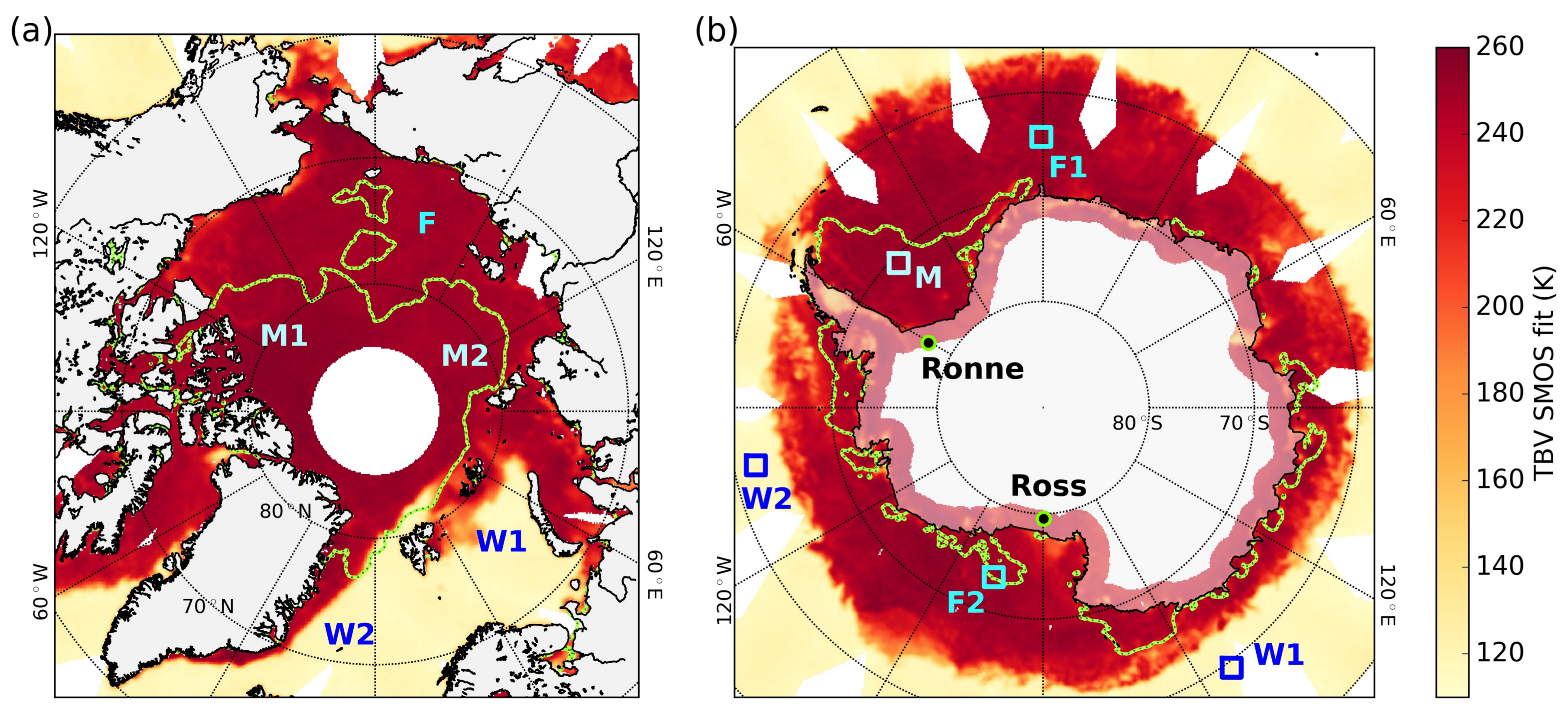
Figure 8.
Brightness temperatures at vertical (top) and horizontal (bottom) polarizations over locations on the Ross ice shelf (a) and on the Ronne ice shelf (b). Data are shown during 30-day periods in 2015 with negligible trends. The different lines are SMOS data at produced using the weighted Zhao fit and a 5-bin mean, as well as SMAP data.

Figure 9.
Timeseries of polarized brightness temperatures in the Arctic averaged over the boxes with (a) first-year ice (box F in Figure 7a); (b) water (box W1); and (c) multi-year ice (box M2). The vertical lines mark the start and end times of the freeze-up period (15 October-15 April) considered for the ice thickness retrieval.

Figure 10.
Two-dimensional histogram of vertically (a) and horizontally (b) polarized TBs from SMAP and SMOS over the Arctic ocean region north of 50 N for the 2-year period from 1 April 2015 to 31 March 2017. Blue lines indicate the respective regression lines.
Figure 10.
Two-dimensional histogram of vertically (a) and horizontally (b) polarized TBs from SMAP and SMOS over the Arctic ocean region north of 50 N for the 2-year period from 1 April 2015 to 31 March 2017. Blue lines indicate the respective regression lines.

Figure 11.
Sea ice thickness (SIT) on 1 November 2015 derived using TBs from SMOS (a) and SMAP (b); gray areas denote saturation of the signal. The rectangle marks the zoom area of SMOS SIT (c); as well as thickness differences between SMOS and SMAP (d) and between SMOS and SMAP with adjusted TB bias (e); (f) histogram of ice thickness differences for all thicknesses between 2 cm and saturation during the considered winter season (15 October 2015–15 April 2016) in the Arctic.

Figure 12.
(a) theoretical dependency of on incidence angle for different cases with constant water salinities and air temperatures at 2 m height assuming a wind speed of 5 m/s during polar night; (b) histogram of SMOS saturation thicknesses retrieved using TBs at near-nadir (0–40) and at during the considered winter season (15 October 2015–15 April 2016) in the Arctic.


Table 1.
Overview of the used fitting methods.
| Method Abbreviation | Method Description | |
|---|---|---|
| 1 | binmean | Fixed incidence angle bins with a width of 1 |
| 2 | optmean | Averaging over incidence angle bins with optimized width |
| 3 | wgmean | Same as optmean, but TBs are weighted by radiometric accuracy |
| 4 | linear | Linear fit of TBs within incidence angle interval with optimized width |
| 5 | simplezhao | Simplified two-step regression based on Zhao et al. [12] |
| 6 | wgzhao | Same as simplezhao, but TBs are weighted by radiometric accuracy |
Table 2.
Average computing times for a single grid point with () measurements.
| Method | Average Computing Time in ms |
|---|---|
| binmean | 0.06 (0.08) |
| optmean | 0.08 (0.11) |
| wgmean | 0.15 (0.19) |
| linear | 0.90 (0.96) |
| simplezhao | 36.6 (58.6) |
| wgzhao | 13.8 (37.0) |
Table 3.
Mean and standard deviations of 30-day time series over two ice shelves for polarized brightness temperatures (TB) from SMAP and from SMOS using the wgzhao and optmean fitting methods.
Table 3.
Mean and standard deviations of 30-day time series over two ice shelves for polarized brightness temperatures (TB) from SMAP and from SMOS using the wgzhao and optmean fitting methods.
| Location | SMOS wgzhao | SMOS optmean | SMAP | ||||
|---|---|---|---|---|---|---|---|
| TB | TB | TB | TB | TB | TB | ||
| Ross ice shelf, 18 May–16 June 2015 | mean (K) | 238.5 | 215.1 | 237.6 | 215.9 | 237.8 | 211.3 |
| 79.52 S, 179.69 E | std (K) | 0.5 | 0.4 | 0.8 | 0.9 | 0.4 | 0.7 |
| Ronne ice shelf, 20 June–19 July 2015 | mean (K) | 233.3 | 211.1 | 231.4 | 212.9 | 232.9 | 206.1 |
| 77.57 S, 29.46 W | std (K) | 0.6 | 0.7 | 0.8 | 1.0 | 0.6 | 0.8 |
Table 4.
Statistics of brightness temperature comparison between SMOS and SMAP over the boxes indicated in Figure 7: correlation coefficient, bias, root mean squared difference (RMSD) (and RMSD after bias adjustment, see text) for daily values over the 2-year period from 1 April 2015 to 31 March 2017.
| Surface Type/Box Name | Correl. Coeff. | Bias (K) | RMSD (K) | |||
|---|---|---|---|---|---|---|
| TB | TB | TB | TB | TB | TB | |
| Arctic | ||||||
| F | >0.99 | >0.99 | 0.7 | 5.0 | 2.0 (1.4) | 5.5 (2.1) |
| M1 | 0.99 | 0.99 | 1.3 | 4.2 | 2.0 (1.4) | 4.9 (2.5) |
| M2 | 0.99 | 0.99 | 0.4 | 4.9 | 2.2 (2.2) | 5.7 (2.8) |
| W1 | 0.31 | 0.32 | −1.2 | 7.0 | 2.0 (1.6) | 7.2 (1.8) |
| W2 | 0.05 | 0.09 | −0.1 | 5.9 | 6.3 (6.4) | 9.4 (7.3) |
| all open water surfaces | 0.16 | 0.14 | −0.8 | 6.5 | 4.1 (4.1) | 8.0 (4.6) |
| all thick ice surfaces in winter | 0.97 | 0.98 | 1.4 | 4.2 | 1.6 (0.9) | 4.3 (1.1) |
| Antarctic | ||||||
| F1 | >0.99 | >0.99 | 0.3 | 5.0 | 1.8 (1.7) | 5.5 (1.9) |
| F2 | >0.99 | >0.99 | 0.8 | 4.7 | 1.4 (0.9) | 4.9 (1.0) |
| M | >0.99 | 0.99 | 1.3 | 4.2 | 1.5 (0.7) | 4.3 (1.0) |
| W1 | 0.66 | 0.57 | −1.2 | 6.3 | 1.6 (1.1) | 6.4 (1.4) |
| W2 | 0.31 | 0.38 | −0.5 | 5.6 | 1.9 (2.1) | 6.0 (2.4) |
| all open water surfaces | 0.48 | 0.46 | −0.8 | 6.0 | 1.7 (1.7) | 6.3 (1.9) |
| all thick ice surfaces in winter | 0.94 | 0.96 | 1.4 | 3.8 | 1.5 (0.8) | 3.8 (1.0) |
© 2018 by the authors. Licensee MDPI, Basel, Switzerland. This article is an open access article distributed under the terms and conditions of the Creative Commons Attribution (CC BY) license (http://creativecommons.org/licenses/by/4.0/).
Share and Cite
MDPI and ACS Style
Schmitt, A.U.; Kaleschke, L. A Consistent Combination of Brightness Temperatures from SMOS and SMAP over Polar Oceans for Sea Ice Applications. Remote Sens. 2018, 10, 553. https://doi.org/10.3390/rs10040553
AMA Style
Schmitt AU, Kaleschke L. A Consistent Combination of Brightness Temperatures from SMOS and SMAP over Polar Oceans for Sea Ice Applications. Remote Sensing. 2018; 10(4):553. https://doi.org/10.3390/rs10040553
Chicago/Turabian StyleSchmitt, Amelie U., and Lars Kaleschke. 2018. "A Consistent Combination of Brightness Temperatures from SMOS and SMAP over Polar Oceans for Sea Ice Applications" Remote Sensing 10, no. 4: 553. https://doi.org/10.3390/rs10040553
Note that from the first issue of 2016, this journal uses article numbers instead of page numbers. See further details here.