Biomass Growth from Multi-Temporal TanDEM-X Interferometric Synthetic Aperture Radar Observations of a Boreal Forest Site


1
Department of Space, Earth and Environment, Chalmers University of Technology, SE-412 96 Gothenburg, Sweden
2
Department of Forest Resource Management, Swedish University of Agricultural Sciences; SE-901 83 Umeå, Sweden
*
Author to whom correspondence should be addressed.
Remote Sens. 2018, 10(4), 603; https://doi.org/10.3390/rs10040603
Submission received: 5 March 2018
/
Revised: 4 April 2018
/
Accepted: 10 April 2018
/
Published: 12 April 2018
(This article belongs to the Special Issue Biomass Remote Sensing in Forest Landscapes)
Abstract
:Forest growth estimation is important in forest research and forest management, but complex to analyze in diverse forest stands. Twelve summertime TanDEM-X acquisitions from the boreal test site, Krycklan, in Sweden, with a known digital terrain model, DTM, have been used to study phase height and aboveground biomass change over 3.2 years based on the Interferometric Water Cloud Model, IWCM. The maximum phase height rate was determined to 0.29 m/yr, while the mean phase height rate was 0.16 m/yr. The corresponding maximum growth rate of the aboveground dry biomass, AGB, was 4.0 Mg/ha/yr with a mean rate of 1.9 Mg/ha/yr for 27 stands, varying from 23 to 183 Mg/ha. The highest relative AGB growth was found for young stands and high growth rates up to an age of 150 years. Growth rate differences relative a simplified model assuming AGB to be proportional to the phase height were studied, and the possibility to avoid a DTM was discussed. Effects of tree species, thinning, and clear cutting were evaluated. Verifications using in situ data from 2008 and a different in situ dataset combined with airborne laser scanning data from 2015 have been discussed. It was concluded that the use of multi-temporal TanDEM-X interferometric synthetic aperture radar observations with AGB estimates of each individual observation can be an important method to derive growth rates in boreal forests.
1. Introduction
Thirty percent of the forested area in the world consists of boreal forests. In Sweden, 51% of the land area is covered by productive forest of mainly boreal or hemi-boreal type, and plays an important role for the Swedish economy. Forests are in particular of major importance for the Earth’s climate through the global carbon cycle [1], and biomass has been identified as an Essential Climate Variable that is needed to reduce uncertainties in our knowledge of the climate system [2].
Interferometric synthetic aperture radar (InSAR) remote sensing systems offer an opportunity to determine three-dimensional properties of forest stands, such as forest height and aboveground biomass, AGB, of importance for inventory and monitoring purposes. The bistatic TanDEM-X system has been shown to be able to determine boreal forest properties with very high accuracy [3,4,5,6,7,8,9,10,11,12,13,14], primarily based on information from the interferometric phase height. The latter depends on tree height, as well as forest density, and is therefore also closely related to stem volume and AGB.
Forest growth estimation is important in forest research and forest management. Models are often developed for even-aged monocultures under traditional management, but there is also a need to estimate growth in more diverse forest stands and conditions. Traditionally, top height of a forest stand is used together with the site index (yield class) and age, to estimate the height change as a function of age, cf. [15,16]. Balzter et al. [17] used SEASAT and JERS-1 L-band radar backscatter and compared with the expected tree growth from general yield class models. However, reduced sensitivity of biomass to backscatter saturation is a severe limitation. The use of single-pass interferometric SAR, InSAR, has opened up the possibility to determine phase height. The latter is here defined as the height relative the DTM of a mean phase-scattering point within the forest canopy, and hence, related to the forest height and determined from the phase difference in the backscattered signals to the two satellites cf. [10]. Phase height is not expected to saturate with increasing biomass. Solberg et al. [18,19] used TanDEM-X together with C-band phase height from SRTM to determine height change and biomass change from 2000 to 2011. Recently, a paper concerning change detection of a tropical forest was published by Treuhaft et al. [20] based on 32 TanDEM-X scenes over a 3.2 year period. The strength of single-pass InSAR is the possibility to determine phase height accurately, due to the elimination of the temporal decorrelation associated with repeat pass InSAR [21].
In previous studies [4,12], methods to estimate AGB from TanDEM-X data and the Interferometric Water Cloud Model, IWCM, were presented and results illustrated a high accuracy in relation to in situ observations from the boreal forest test site Krycklan, in Sweden. The main goal of this paper is to investigate AGB growth and change of individual stands over a 3.2 year period of TanDEM-X data from Krycklan. AGB growth is estimated using IWCM, and compared to the in situ information from 2008 and airborne laser scanning, ALS, data from 2015. With TanDEM-X, we obtain three observables, backscatter, coherence, and phase height. From these observables, we estimate the stem volume and biomass from IWCM using allometric relations between general forest properties. The model compensates for differences in the observations caused by varying weather effects and varying baselines between the two satellites and depending on the specific forest conditions through the allometries. An alternative to IWCM using allometry is to use known reference stands in the area to compensate for such effects, e.g. [3,13,22]. In a recent publication [23], National Forest Inventory, NFI, plots were used together with TanDEM-X observations to determine AGB over the entire of Sweden, assuming proportionality between phase height and biomass. IWCM gives a more detailed relation between TanDEM-X observables and stem volume/biomass, and is not dependent on reference stands for training (some stands are, however, useful for verification purposes). IWCM was applied to Krycklan data in [4], without the use of local reference data for training, and the results will, in this paper, be used for estimating biomass change for individual stands. To detect management actions during the time period, we have used SPOT-5 and aerial photos for comparison.
2. Materials and Methods
2.1. Main Dataset
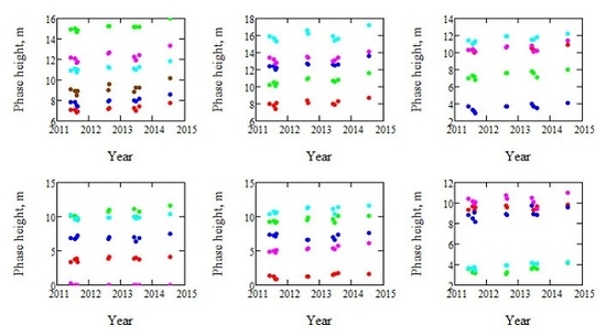
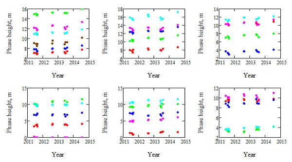
A large number of TanDEM-X acquisitions were available for Krycklan, which is a boreal forest reference site and located in northern Sweden (lat. 64.150N, long. 19.460E). Acquisitions analyzed in this paper have been analyzed before in different contexts, particularly in [4], where the estimation of AGB used in this paper is presented, but also in [9,10,11,14]. The acquisitions considered in this paper were all from orbit 9 with an incidence angle of 41°, passing over Krycklan at 16:12 UTC. Only the VV polarization was investigated in order to keep the polarization state constant, and only summer acquisitions were used to keep the retrieval conditions as constant as possible. The scene center spatial resolution of the TanDEM-X data is 1.8 m in ground range and 6.6 m in azimuth, but the data are averaged over stands with size varying from 2.4 to 26.1 ha. The spatial grid of the DTM used for estimation of phase height is 2 m. The meteorological conditions varied between the acquisitions [4], and also the height of ambiguity (the height interval for which the interferometric phase increases from 0 to 2π), HoA, which varied between 36 and 60 m. The phase heights of the 31 forest stands of 12 TanDEM-X observations acquired over 3.2 years are shown in Figure 1.
2.2. Method for Interpretation of TanDEM-X Dataset
The method for interpretation of the TanDEM-X dataset was the Interferometric Water Cloud Model, IWCM, which is a semi-empirical model for radar scattering from a forest. IWCM is characterized by a number of parameters related to radar scattering, the radar backscatter associated with ground, σgr, and the vegetation layer, σveg, the two-way attenuation, α, back and forth through the medium with a height h, exp(−αh), and η, the area-fill, which is the fraction of the area covered by vegetation which attenuates the microwaves.
The phase height, Figure 1, which is central in the analysis below, is determined by the observed phase difference of the backscattered waves at the two satellites, and represents the weighted mean height of the scattering center in the forest. The height of ambiguity, HoA, is also an important parameter in IWCM. The TanDEM-X coherence represents the correlation between the scattered wave components from the ground and the vegetation layer to the two satellites [24,25,26,27]. The coherence associated with the zero phase height is denoted γsys, and is due to system noise. The phase height and coherence are expressed in IWCM as functions of α, σgr, σveg, γsys, HoA, and the stem volume, V, and the backscatter as function of α, σgr, σveg, and V.
In order to match the model to the TanDEM-X observations and determine the parameters, we traditionally train models by fitting the model to forest areas with known properties. However, it was shown in [4,5,12] that an alternative to knowledge of local conditions is to use allometry typical for large forest areas or a particular type of forest. For IWCM, we use allometry for the relation between the basal area weighted mean height, Lorey’s height, and stem volume, h(V), between area-fill and stem volume, η(V), and between biomass and stem volume, AGB = BF V, where V is the stem volume and BF is a biomass factor, here assumed constant, relating stem volume and biomass aboveground, but excluding stump. For h(V), we used a relation which is characteristic for forest in Sweden, see [27,28].
The allometry used for Krycklan was the same as for Remningstorp, a test site located 700 km south of Krycklan, see Figure 2, in order to avoid site specific data. For BF, the constant value of 0.51 Mg/m3 was used, a factor that varies with species composition and age [29]. For η(V), an expression based on ALS observations of the vegetation ratio in Remningstorp was used [3], cf. also [30],
where η(V) is related to the horizontal density of trees, species, and age. In Figure 2, the allometric relations are illustrated together with the data from Krycklan. IWCM is based on allometry, which is supposed to be general for the type of forest studied. In Krycklan, we have the possibility to verify the allometry relative the local data, see Figure 2, illustrating the relevance of the allometry, and thus, also for the inversion based on IWCM. For further details about IWCM, see [5,27,31,32], and as applied to data from Krycklan [4].
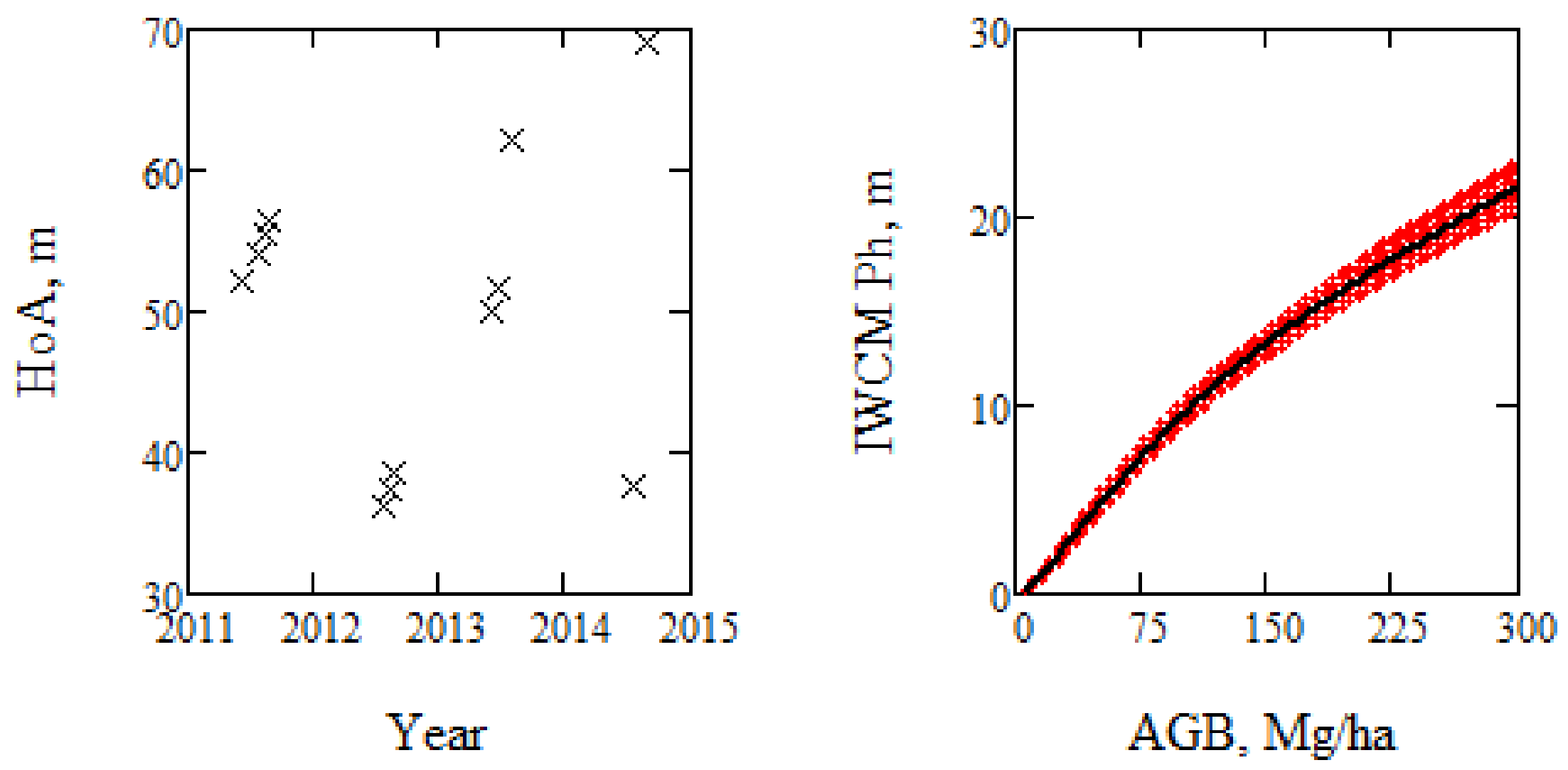
The TanDEM-X phase height (with a DTM subtracted), coherence, and backscatter, were determined in [4] as mean values over the 31 forest stands from BIOSAR 2008 [33], or in practice 29 stands, since two had been clear cut before the start of the TanDEM-X observations on 17 June 2011. The model was fitted to the variation between the forest stands of phase height, coherence, and backscatter for each of the twelve TanDEM-X VV summer acquisitions during 2011–2014. For the growth analysis in this paper, two winter cases are excluded, since they were characterized by a snow layer on the ground, which causes effects not taken into account by IWCM. The mean properties and standard deviation of the IWCM parameters are listed in Table 1, and the derived results by means of IWCM for the phase height according to [4] is illustrated in Figure 3.
In IWCM, stem volume, V, is the primary quantity, and height and stem volume are related by the allometric relation h(V). From the derived stem volume, we determine the model height, hM(V) which is closely related to Lorey’s height in the case of a homogeneously dense forest. However, in the case of thinning both AGB and hM will decrease, but Lorey’s height may remain. Finally, the stem volume and biomass of each stand was estimated from observations of phase height, coherence, and backscatter by the method presented in [4] with RMSE relative to the BIOSAR 2008 in situ AGB-values ranging between 16 and 22%. The RMSE was observed to increase with time, due to growth and other changes in the stands.
It is clear from Figure 3 that an increase of phase height is related to an increase in AGB in a nonlinear manner related to variations in forest properties and TanDEM-X parameters.
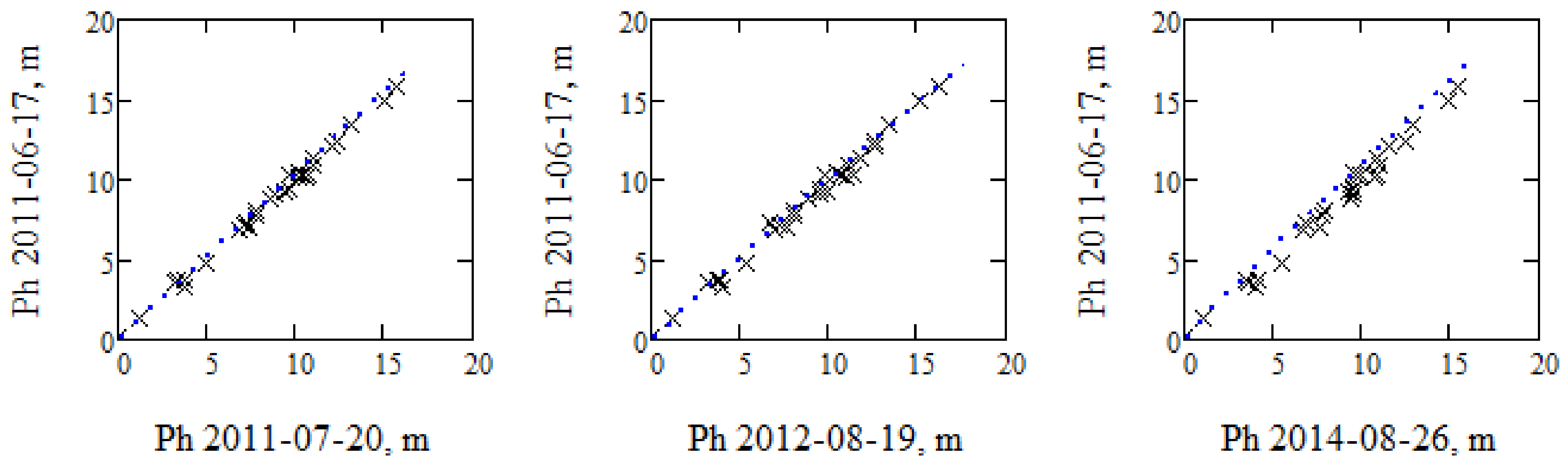
Each TanDEM-X observation is analyzed separately using IWCM. In Figure 4, we compare the phase height measured in the first TanDEM-X acquisition with three other acquisitions, in order to illustrate the linear relation between the observations. The dotted lines are the IWCM estimated phase height expressions. The difference is a measure of how accurately IWCM estimates the phase height. The figure illustrates that the observations are very stable over time, and IWCM is a good model that fits the individual observations and also agrees when observations and models are compared over time, i.e., properties of importance for time change analysis.
2.3. Supporting Dataset
2.3.1. Field Data from 2008
We used field data from the forest research site Krycklan, which consists of a 6800 ha large river catchment. It is a boreal forest landscape dominated by coniferous trees and with terrain height varying between 130 and 380 m. Krycklan is an area with both nature reserves, and many different forest owners with varying management practice. The prevailing tree species are Scots pine (Pinus sylvestris L.; mainly in dry upslope areas), Norway spruce (Picea abies (L.) Karst.; mainly in wetter, low-lying areas), and birch (Betula spp., in the riparian forest along larger streams).
For the BIOSAR 2008 experiment [33], 31 forest stands were selected with a uniform stratification with respect to biomass and ground slope, since it was expected that ground slope would influence remote sensing data and biomass was in focus for the investigation. The size of the stands varied between 2.4 and 26.1 ha, and in situ data were inventoried. Field plots were distributed within the 31 stands with a systematic spacing of 50–160 m, depending on the size of the stand. The spacing in each stand was determined with the aim of obtaining 10 plots in each stand. The resulting number of plots for all stands varied between 8 and 13, with an average of about 10 plots per stand. In total, 311 field plots were established within the 31 stands investigated. On the plots with 10 m radius, all trees with a diameter at breast height DBH ≥ 0.04 m were calipered, and the species identified. Height and age were also measured of randomly selected sample trees (selected with the probability proportional to basal area) using a hypsometer and a drill. On average, 1.5 sample trees were selected per plot. The average AGB was determined on plot-level using established biomass functions valid for Swedish forests [34,35].
2.3.2. Field Data from 2015
A large survey of Krycklan took place 2015, see e.g., [36], when 556 circular plots with 10 m radius were distributed in a regular grid covering the complete catchment and surveyed. Of the plots, 424 were located in the forest. Unfortunately, the plots from 2008 were not inventoried. ALS data over the test site was also collected in August 2015 with a Titan L359 laser scanner with more than 20 points/m2 density.
2.3.3. Methods for Biomass Estimates from 2015
Estimating in situ biomass can be carried out by different methods. Current state of the art encompasses a field inventory at plot level, which can be extrapolated by using a wall-to-wall coverage of ALS data. ALS observables, such as height percentiles and ratios, are linked to the field inventoried estimates of biomass. The estimates of biomass are determined with allometric equations [37,38,39] for respective species, which are expressed in diameter at breast height, DBH, and tree height. The height of each tree was estimated from DBH with a function calibrated using local tree height measurements. We will here denote AGB estimates with these models as Marklund’s. In BIOSAR 2008, biomass was estimated using similar yet slightly different allometric models [35], which also required some additional explanatory variables. These included north coordinates, age at breast height, site index, and the last five year’s radial increment as an independent variable. The latter is often not measured in field, and then has to be estimated from the height, age, and site index. Estimates based on these models are denoted Petersson’s.
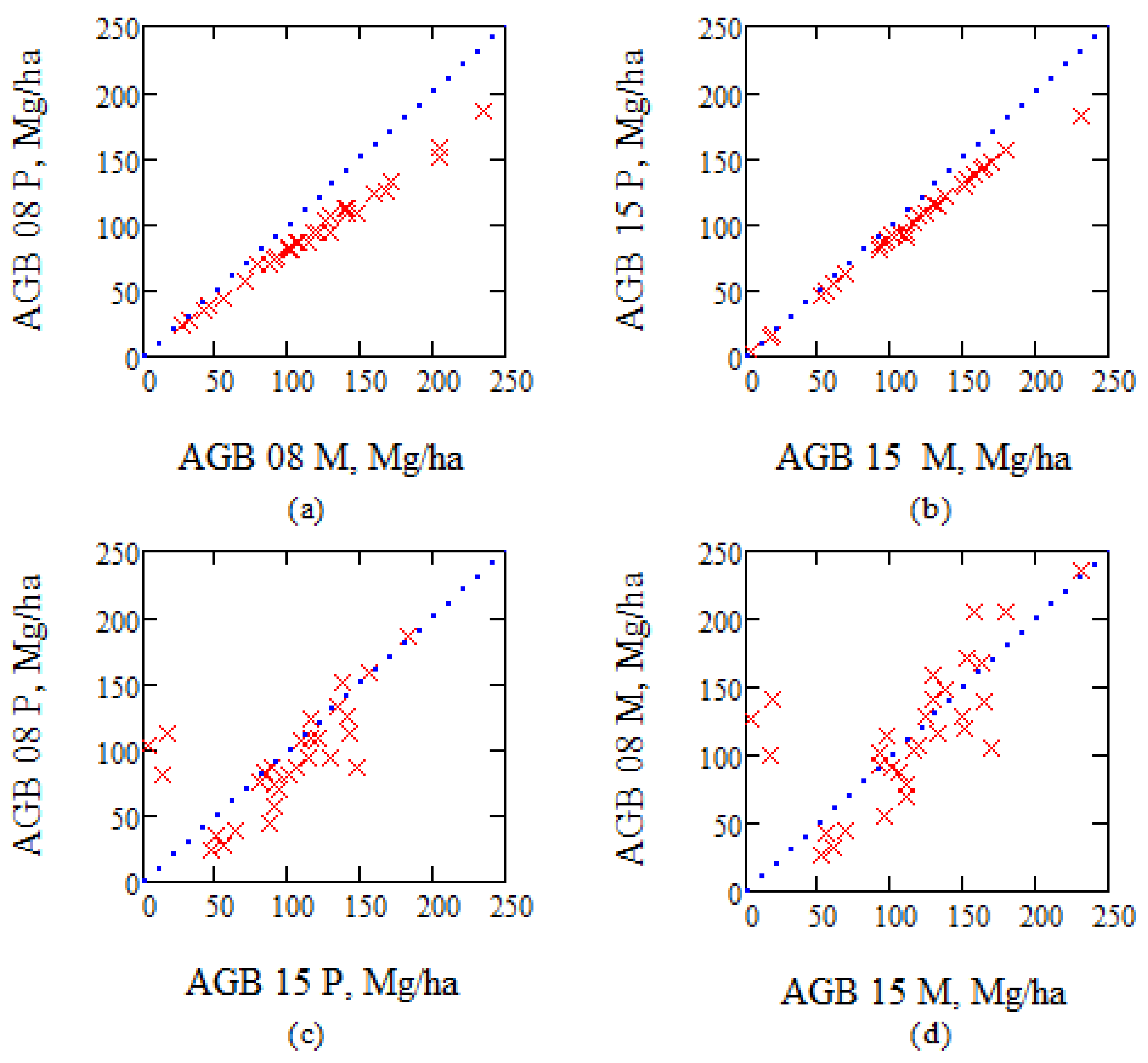
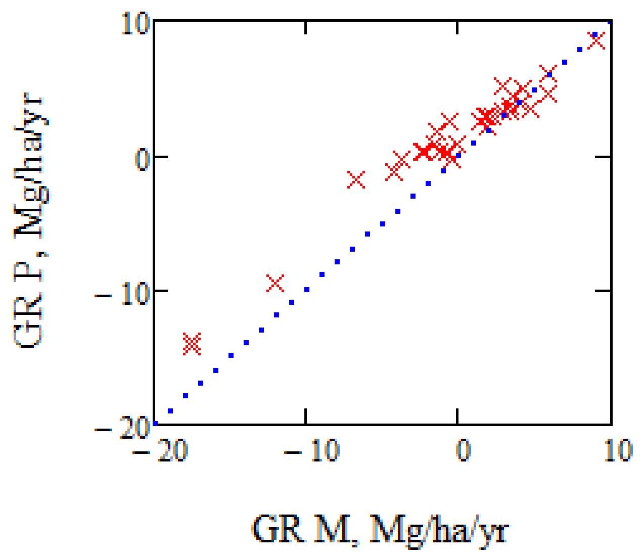
In the current study, biomass was estimated according to the formulas of Petersson (P), as well as Marklund (M) from the in situ data from 2008, and for the corresponding ALS data in 2015 (other in situ plots were complemented with ALS data to obtain estimates of the same stands as in 2008) based on the 424 plots with 10 m radius. The accuracy is estimated to be 14%, and results are illustrated in Figure 5, and the annual growth based on either Petersson or Marklund data are compared in Figure 6.
Figure 5 and Figure 6 illustrate how the reference biomass and biomass change are affected by using different allometric models. Since they show a notable difference, we suggest that the accuracy of reference data should be further investigated in future studies, in order to assign the major observed uncertainties to the remote sensing data or model.
3. Results
The goal of this section is to determine the change in biomass over time based on the TanDEM-X data based on IWCM, and to analyze different reasons for change, and finally to discuss the relation to the in situ and ALS data.
3.1. Linear Regression Results
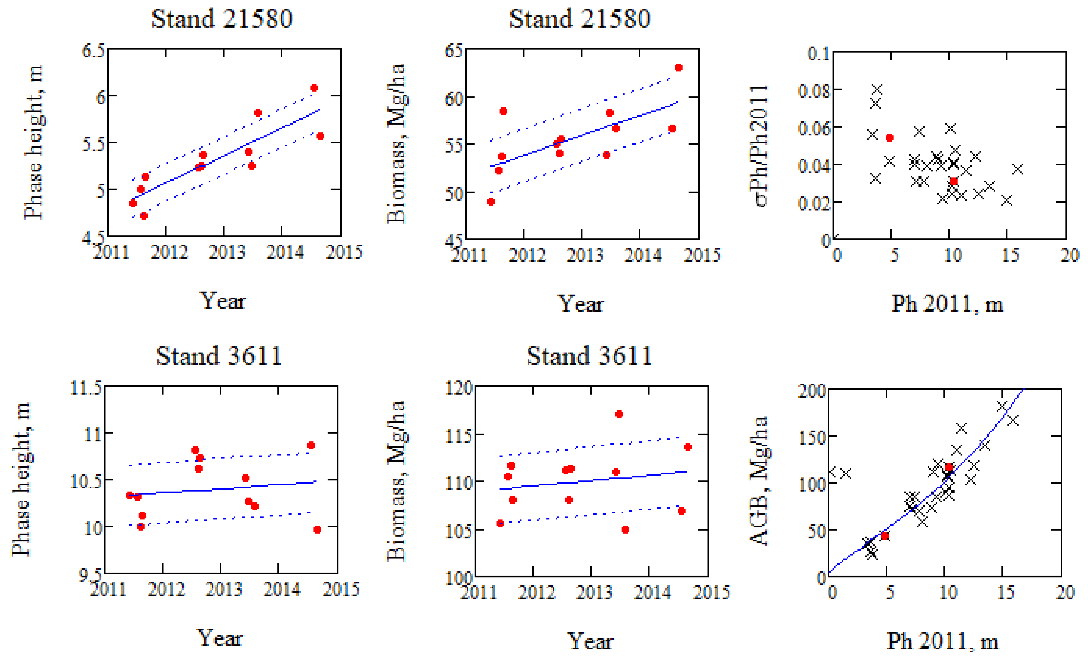
The change of phase height and biomass over time of each stand is determined with linear regression of the observations, which also means that the variations of individual estimates are smoothened. In order to illustrate the change in more detail, the stand with the highest phase height change (stand 21,580) is illustrated in Figure 7, together with the stand with the lowest phase height change (stand 3611), although not negative, which would indicate manual impact on the stand.
The mean phase height rate was determined to 0.16 m/yr, and the mean growth rate to 1.9 Mg/ha/yr for 27 stands with non-negative growth rates, and with biomass varying from 23 to 183 Mg/ha. The spread around the linear regression line, ± one standard deviation, is included as dotted lines in Figure 7, and the standard deviation is 0.20 m and 1.40 Mg/ha in the high growth case, and 0.32 m and 1.82 Mg/ha in the low growth, but higher AGB case. The one standard deviation variability of Ph and AGB are both varying between 2% and 10% relative to the values for 17 June 2011.
3.2. Interpretation of Linear Regression Results
Since IWCM gives the expression for the phase height Ph, and its dependence on stem volume V, we can determine theoretical values for growth of AGB and the related mean height hM as determined from the phase height growth. As the phase height varies with stem volume somewhat differently for each TanDEM-X acquisition, we use the mean values of the IWCM parameters of all TanDEM-X acquisitions, cf. Table 1, and approximate with Ph_mean(V)
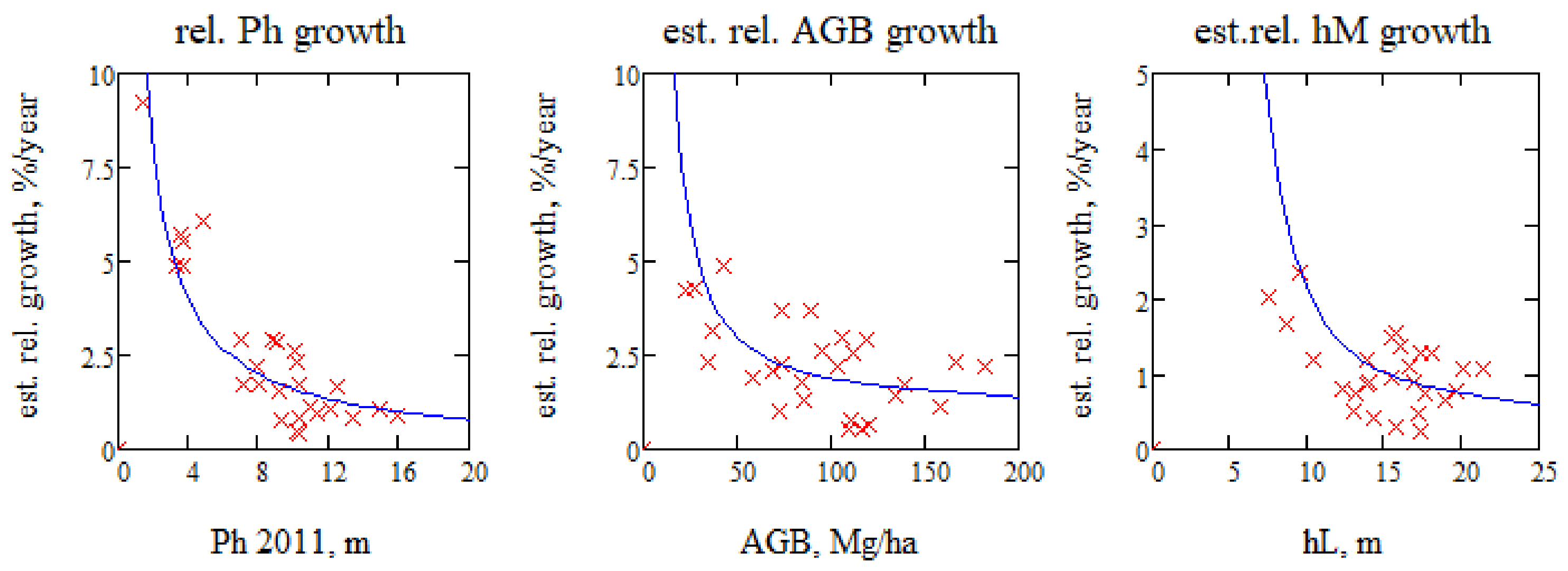
The slope of the linear regression line of phase height as function of time represents the change per year, and we approximate dPh/dt with the mean value for all the forest stands, neglecting, for the moment, changes in the IWCM parameters. The relative growth of phase height, as determined by linear regression, is illustrated in Figure 8, and expressed in %, i.e., 100, and similarly for biomass and mean height, as determined by (3) and by (1). Ph is normalized by the phase height of the first TanDEM-X acquisition 2011, and AGB and mean height hM are normalized by the in situ values for AGB and Lorey’s height, hL, from 2008. Figure 8 illustrates that the relative phase height growth rate is higher for the stands with low phase height, i.e., the young stands, relative those with higher phase height, cf. [20].
AGB Approximately Proportional to Phase Height
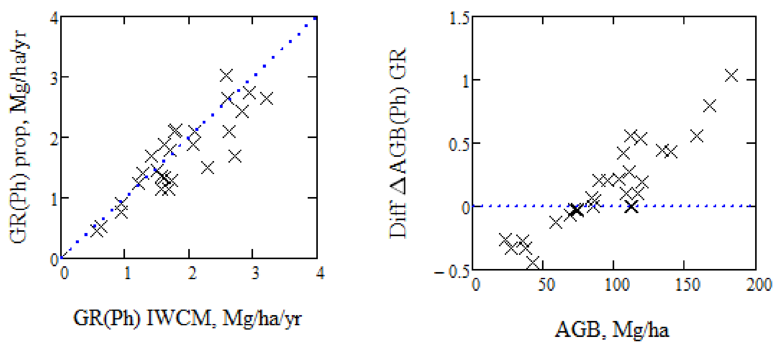
In Figure 9, we have illustrated the AGB growth rate, GR, as determined from the growth rate of phase height, on one hand assuming a proportionality between phase height and AGB, AGB = κpr Ph with κpr = 10.3, and on the other hand AGB as determined from IWCM from (3), and based on the first TanDEM-X acquisition. The difference in growth for the individual stands varies from −40% to +20%. Assuming AGB proportional to phase height means that the AGB growth is proportional to phase height growth. The difference in expected AGB growth relative IWCM results is seen to vary with AGB, due to the non-linear variation between Ph and AGB of the stands.
An important question is if we can estimate the biomass change from the phase height change. If so, we may avoid the need for a DTM if we are only interested in the biomass change. However, we must first establish the relation between AGB and phase height, i.e., determine κpr, and for that purpose, we need to know the phase height. Since the phase height is related to the product of vegetation density and height, phase height will vary between different forest types. In addition, we have changes associated with changes in radar scattering, change of HoA, etc. For the 12 summer acquisitions from Krycklan, we have a variation of κpr between 9.5 and 10.8, indicating the variability of the relation between AGB and phase height.
3.3. Ratio between AGB Change and Phase Height Change Using IWCM
The phase height change can be estimated from a sequence of TanDEM-X acquisitions, but the important quantity to determine is the AGB change, and we want a relation between the ratio between ΔAGB and ΔPh. Phase height is a function of stem volume, V, but also influenced by the model parameters α, σgr, σveg, and HoA (most influential of the model parameters is α). We now introduce the ratio factor RF, cf. [20], the ratio between the AGB growth rate and the Ph growth rate according to IWCM
We may consider the changes in the model parameters as error terms, since they are varying randomly, and RF(V) is illustrated in Figure 10, together with measurements for each individual stand. The theoretical curve is determined according to (4) based on an assumed phase height determined by the mean properties of the acquisitions, see Table 1. If AGB is proportional to Ph, then RF will be constant. From Figure 10, we see a difference between the results when AGB is derived from each TanDEM-X acquisition using IWCM and linear regression of the phase height changes (marked by x), and the AGB changes derived from (4) based on the conditions associated with a single acquisition using mean parameter values (dotted line), and finally, when AGB is proportional to Ph (dashed line). The best alternative to estimate AGB change from Ph change is to estimate AGB for each acquisition, while the use of the properties of a single TanDEM-X acquisition is less accurate, cf. the variation of phase height as illustrated in Figure 1 and Figure 3, and to use an assumption that AGB is proportional to Ph is still less accurate.
3.4. Changes Related to Manual Impact and to Tree Species
3.4.1. TanDEM-X Observations of Change, e.g., Clear Cutting or Thinning
Managing the forest includes clear cuts of stands, but also thinning at regular times in order to increase the value of the forest by optimizing certain properties, e.g., increasing the amount of tall straight trees suitable for wood constructions. Such changes affect the InSAR measurements differently. Clear cuts are easy to detect from an abrupt phase height change, and also, change of coherence and backscatter. Thinning is more complex, since it affects the forest differently. The most common thinning in Sweden is to cut suppressed trees and leave larger trees, but sometimes the larger trees are cut to let the smaller trees grow. In the InSAR model approach, the stem volume variation is related to the TanDEM-X observables governed by the height and density allometries. If either the mean height or the density is changed by thinning, the phase height will decrease as well as the estimated stem volume.
Negative or small phase height slopes or AGB slopes over the investigated time period or a large variability may indicate that a change, possibly thinning or clear cut, has taken place; see the behavior of stands denoted 1474, 3611, 4038, 4451, and 36,169 in Figure 11. We investigate AGB changes, since the estimated AGB should be compensated for variations in HoA and IWCM parameters. Besides stands 1474 and 4451, large variability was also found in stands 3611 and 36,169, with a possible thinning during summer 2013. Stand 4038 does not show a clear change from inspection of the figure, but a large variability in relation to the slope.
In addition to TanDEM-X information, we have SPOT-5-HRG scenes from 31 August 2008 and 26 July 2014, the latter with partial coverage. Aerial photos were available from 2009, i.e., before the TanDEM-X acquisitions, and 29 May 2013. From the SPOT images and aerial photos, the thinning of 1474 was verified as having taken place in the aerial photo 29 May 2013, although the detection was somewhat uncertain, due to the vegetation season and since the stand includes a mixture of tree types (41% Scots pine, 33% deciduous, 26% Norway spruce). The possible changes of 3611 and 36,169 occurred after 29 May 2013, and were not covered in the SPOT 2014 image. The reason for the variability of stand 4038 is unclear. Stand 4451 is a clear cut.
Three important storms (named Berit, Dagmar, and Hilde) took place during the period, but the 10 min wind average was limited in the area to 6.7 m/s (26 November 2011), 8.2 m/s (26 December 2011), and 10.3 m/s (17 November 2013) in Petisträsk, 40 km north, and no obvious effect has been observed in Krycklan from the TanDEM-X observations.
3.4.2. TanDEM-X Growth Related to Tree Types and Age
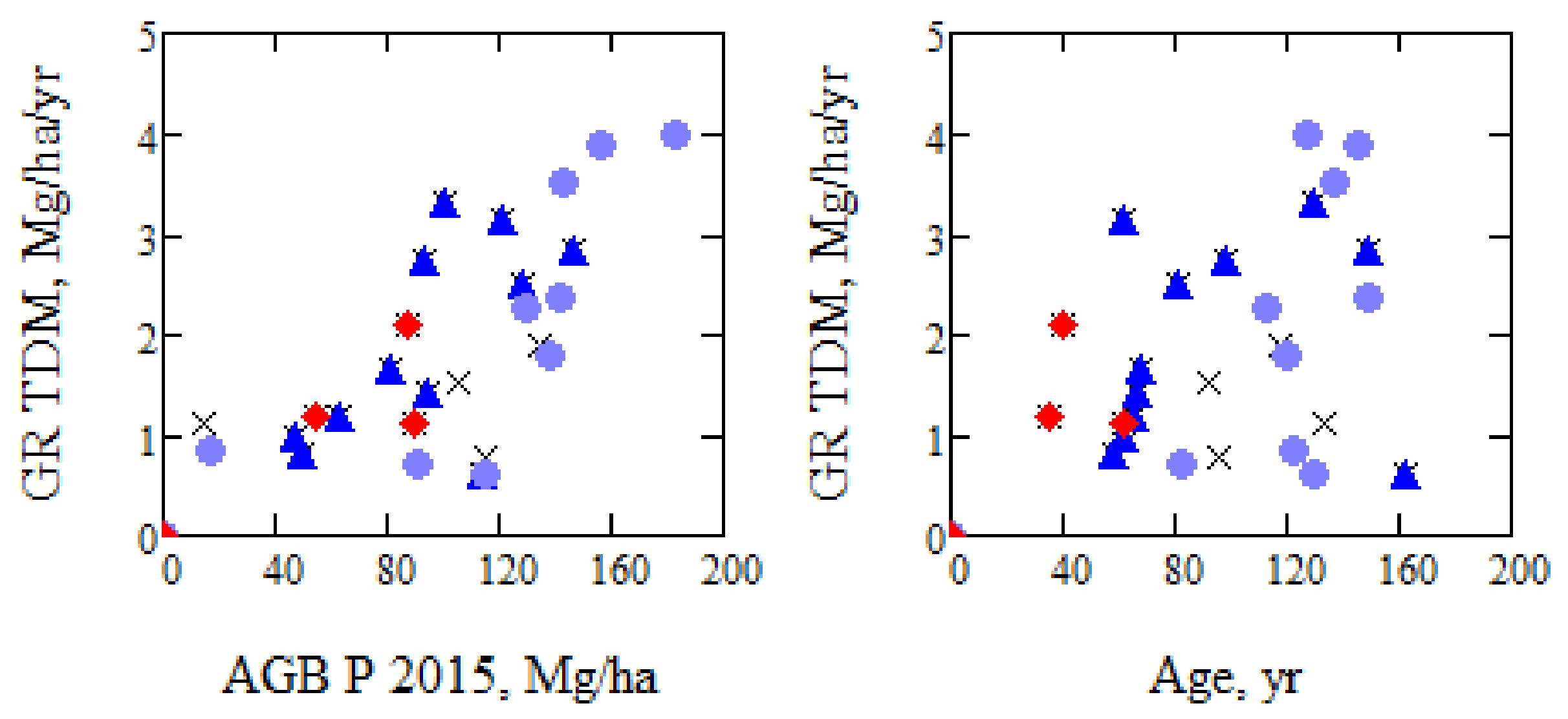
Some of the changes we are interested in are expected to be dependent on tree species and on age. The prevailing tree species are, according to [9], Scots pine (Pinus sylvestris; mainly in dry upslope areas), Norway spruce (Piceas abies (L.) Karst: mainly in wetter, low-lying areas), and birch (Betula spp.; in the riparian forest along larger streams). In Figure 12, the estimated growth rate, GR, is illustrated, and we mark stand values by x, and those stands with >60% Picea with an additional dark blue triangle, those with >60% Pinus with light blue dots, and those with at least 30% deciduous with red diamonds.
From Figure 12, the young stands with >30% deciduous show high growth, and young Pinus tends to grow faster than Picea, while old Pinus grow slower than Picea, in line with practical experience. Four stands with an age in the interval 123–162 years have a low growth rate (0.6–1.1 Mg/ha/yr) which for three (ID = 3611, 3689, and 15,100) can be related to suspected thinning summer 2011, 2013, and 2012, respectively. Stand 1764 (age 162 years) is clear cut before 2011, and the age is then incorrect.
It is hard to draw conclusions regarding growth of different species, since the site properties vary and we do not have stands with dominating species in all AGB intervals. This also illustrates the need for satellite information on growth results for different stands. From literature related to forest growth, see e.g., [15,40,41,42], we typically find a low growth rate for small as well as high stand age. The present results show a high growth rate in the interval 60–150 years of age.
3.5. Comparison with Other Datasets
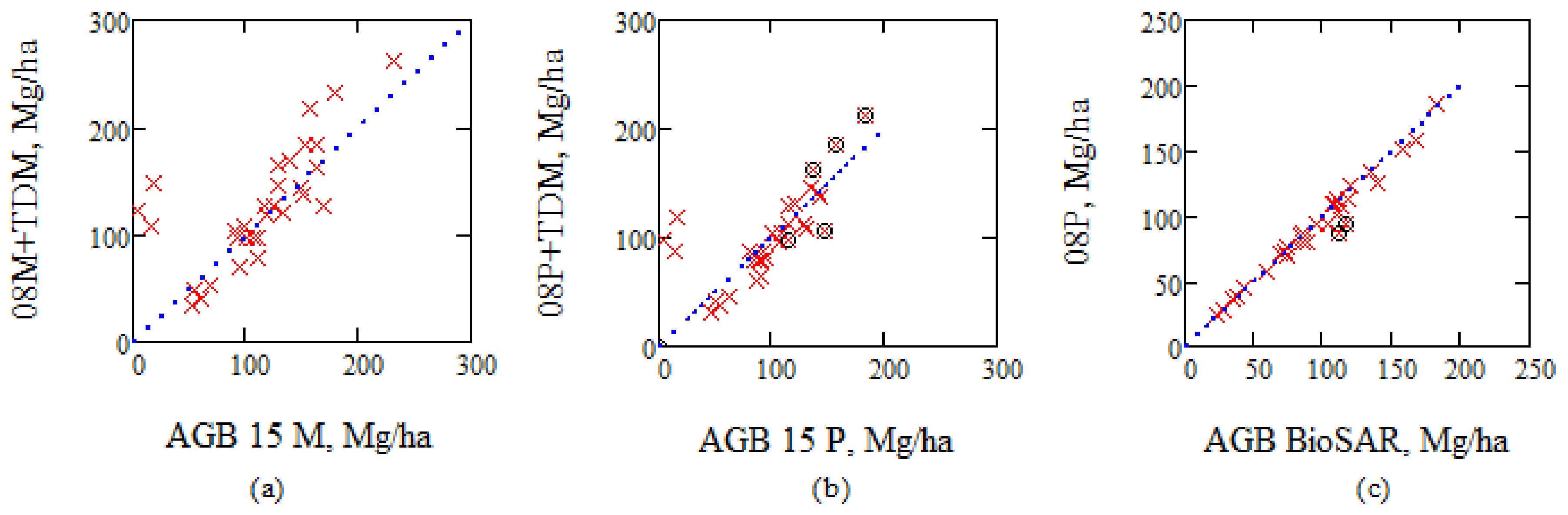
One way to illustrate the TanDEM-X/IWCM results is to update biomass estimates from in situ estimates from 2008 by the annual growth rates for individual stands according to TanDEM-X/IWCM, and compare with ALS estimates from 2015, see Figure 13a,b. A slightly better agreement is found with estimates based on Petersson’s model compared to Marklund’s model.
The model by Petersson was used in BIOSAR 2008, but the outcome is slightly different, since the Petersson’s model includes variables not measured in the in situ data or which are not available for every tree, and hence, have to be modeled (i.e., radial increment and age), see Figure 13c. In particular, two stands (ID 3611 and 30,097) show a 20% difference. These two stands 3611 and 30,097 are marked in Figure 13c, and also in Figure 13b, in addition to three stands with highest AGB (ID 2269, 3245, and 3715) since Figure 5c,d indicate none or negative growth i.e., some manual effects may have taken place between August 2014 and August 2015, when also one clear cut took place in addition to the two earlier that have taken place since 2008. From Figure 13b, we find relatively good agreement between the compared values using the TanDEM-X/IWCM growth rates.
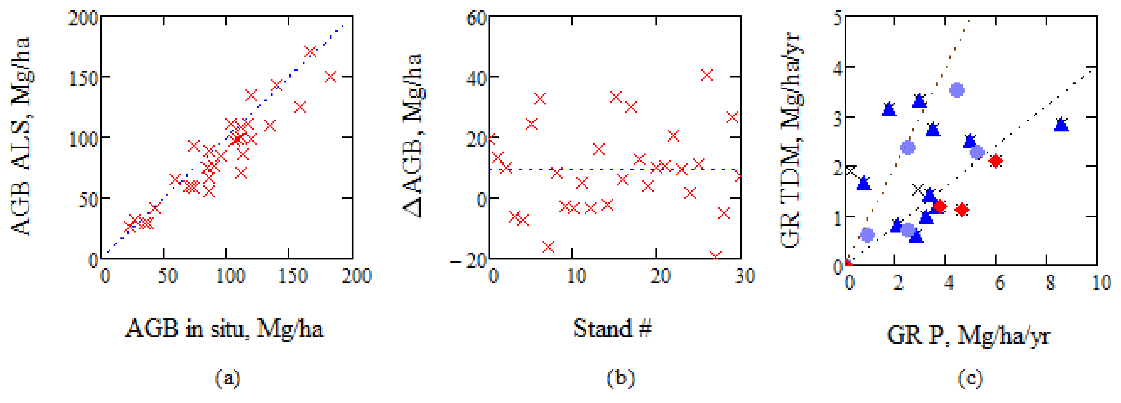
To further illustrate the problem of using ALS estimates as reference for biomass growth, we use information from BIOSAR 2008 when in situ as well as ALS estimates were used, see Figure 14a. ALS was trained on stands covering a large part of the area in Krycklan. RMSE for the 31 stands is 18% or 17 Mg/ha. When we analyze the difference between the AGB estimates, we find that there is an offset of 9 Mg/ha and a spread from +41 to −19 Mg/ha. The ALS estimates from 2015 have an RMSE relative in situ value of 14%, due to higher point density, and the spread can then be expected to be somewhat lower, but still essential for growth estimation. The growth estimates of TanDEM-X/IWCM compared to ALS using the model by Petersson is illustrated in Figure 14c.
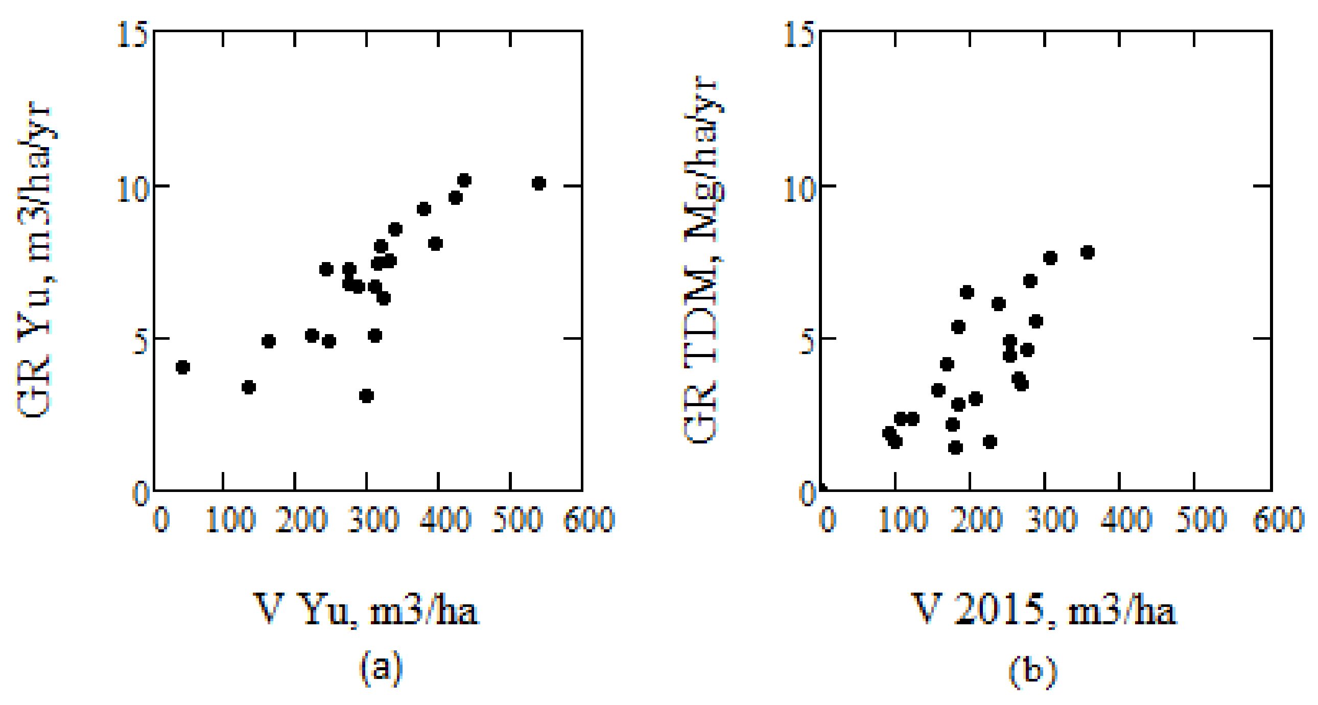
To estimate growth using ALS-estimated AGB can be problematic, and the need for multi-temporal ALS observations was pointed out in e.g., [43]. In [43], combined ALS observations from 1998, 2000, and 2003, together with three different techniques to determine growth, a method based on individual tree top differencing, digital surface model differencing, and canopy height distribution differencing, were used. Their observations from Kalkkinen, 130 km north of Helsinki (and approximately 450 km SSE Krycklan), listed in Table 1 in e.g., [43], are illustrated in Figure 15 after division by 5, to compensate for their five year growth estimates. We conclude that the growth rate tendency as a function of stem volume between the results for Kalkkinen and TanDEM-X/IWCM for Krycklan, taking into account the difference in latitude between Krycklan and Kalkkinen, are similar.
The difference between the models by Marklund and Petersson to estimate biomass, the lack of in situ data from 2015, differences between in situ and ALS estimates of biomass, and the only partly overlapping time intervals caused problems in comparing the ALS growth results with TanDEM-X/IWCM. In spite of these reservations, Figure 13b and Figure 14c indicate a relatively good agreement between TanDEM-X/IWCM results, and ALS 2015 observations based on the model by Petersson. Our results suggest that we still need a better understanding of error sources associated with the in situ estimates as well as remote sensing techniques, cf. [44]. More comparisons between multi-temporal TanDEM-X and in situ/ALS observations simultaneous in time are important for future developments.
4. Discussion
We have studied 12 summer acquisitions of TanDEM-X VV-polarization data from the same orbit and determined growth using linear regression over the 3.2 year period 2011–2014. IWCM has been used to determine the growth rate of 29 boreal forest stands, and the results have been compared with SPOT-images, aerial photography, ALS and in situ data.
Estimates of AGB with IWCM and TanDEM-X data depends on the allometry h(V) and η(V). We have shown that h(V) agrees well with local data, and that η(V) is in line with the ALS vegetation ratio. IWCM is used to estimate AGB of each stand for each TanDEM-X acquisition and the phase height observations, and model estimates of phase height shows a consistent behavior over the 12 acquisitions.
The derived growth rates vary with AGB, and it is found important to estimate AGB from IWCM (i.e., using phase height, coherence, and backscatter) for each individual TanDEM-X acquisition, and determine the growth from a linear regression over the estimated values, in order to reduce variability of the individual estimates. The relative growth rate is found to be highest for young stands with low AGB, but the absolute growth rate is high up to stands with 150 years of age. A simplified model based on a proportionality assumption between AGB and phase height was shown to provide different and less accurate results.
Since the phase height is the important TanDEM-X (or bistatic InSAR) observable for biomass estimation, a DTM is necessary to determine the height difference between the phase center and the ground. To determine biomass change directly from a phase height change would give a biased result in the studied case, due to the nonlinear relationship between phase height and AGB, and due to variation of microwave scattering properties. This means that phase height variation alone is not sufficient to analyze AGB change, but also coherence and backscatter needs to be included in order to determine AGB for each of the TanDEM-X acquisitions.
The growth rate is influenced by weather and climate properties, solar illumination conditions, precipitation, mortality, storms, and silvicultural practices, to mention some effects. In situ measurements, as well as ALS, are expensive, and satellite observation is therefore a preferred alternative, provided that the accuracy is adequate. TanDEM-X observations interpreted with IWCM using a DTM and specific allometries for forest properties, therefore offers a possibility for growth rate estimation.
The demand on accuracy of the verification information from e.g., ALS, is high, and associated problems have been demonstrated and discussed. In situ observations in parallel with TanDEM-X observations or possibly multi-temporal ALS observations seem to be necessary, in order to determine the accuracy of the proposed method. However, the results have been illustrated and compared with the available in situ and ALS observations with acceptable agreement, and the demands on a future verification process discussed.
So far, the only analysis on short term forest AGB change by means of TanDEM-X observations is presented by Treuhaft et al. in [20], and applies for a tropical area. Solberg et al. [18,19] have investigated long term forest change for REDD (reducing emissions from deforestation and forest degradation) applications for a tropical area using TanDEM-X data compared to SRTM data from 2000, which is a different problem, with other complications and other demands on accuracy. In tropical areas, a DTM is normally not available today, which complicates the estimation of phase height. Finally, an analysis of forest height change and canopy density change for a hemi-boreal site using TanDEM-X observations and the TLM method has been presented in [45].
In the future, the Global Ecosystem Dynamics Investigation, GEDI, Lidar project planned for ISS 2018, and the TanDEM-L with planned launch in 2022 will provide new and interesting information in conjunction with TanDEM-X and IWCM.
5. Conclusions
TanDEM-X, DTM, and IWCM (without the use of local data for training of the model) were studied. Phase height and biomass of 29 stands for a time span of 3.2 years 2011–2014 were analyzed to determine the linear trend or the growth rate for 29 stands. The linear regression means averaging over the individual observations, and an associated improved accuracy. In this paper, 12 summer TanDEM-X acquisitions were used, from which the mean phase height rate was determined to be 0.16 m/yr and the mean growth rate to 1.9 Mg/ha/yr for 27 stands varying from 23 to 183 Mg/ha. The maximum phase height rate was 0.29 m/yr and the associated AGB rate 4.0 Mg/ha/yr. The growth rates were found to vary with AGB with the highest relative growth rate for young stands, and a high absolute growth rate up to an age of 150 years.
It was illustrated how lack of a DTM or an assumption of proportionality between AGB and phase height gives a biased AGB change estimate. In addition, each TanDEM-X acquisition should be used to estimate AGB using IWCM by not only phase height, but also coherence and backscatter. The site productivity, as derived from TanDEM-X, agrees with expected results for the region and from ALS observations. The species dependence of the growth rates was studied, and some conclusions, in line with general experience, could be drawn.
It is concluded that the use of multi-temporal TanDEM-X observations with AGB derived from each individual observation can be an important method to derive growth rates in boreal forests.
Acknowledgments
ESA and the BIOSAR 2008 team are gratefully acknowledged for funding and collecting the forest ground data for 2008, Swedish Research Council for sustainable development, Formas, and the Swedish National Space Board, SNSB, for 2015. DLR is acknowledged for TanDEM-X data distributed through proposal XTI_VEG0376 3D Forest Parameter Retrieval from TanDEM-X Interferometry (L.M.H.U. PI). Maciej Soja is acknowledged for support with processing the TanDEM-X data. This work was partly funded by SNSB Grant 164/16.
Author Contributions
All authors participated in detailed discussions and in writing of the paper. J.I.H.A. proposed the paper, analyzed TanDEM-X data and wrote most of the paper. H.J.P. studied ALS, SPOT and aerial photos.
Conflicts of Interest
The authors declare no conflict of interest.
References
- Houghton, R.A.; Hall, F.; Goetz, S.J. Importance of biomass in the global carbon cycle. J. Geophys. Res. Biogeosci. 2009, 114. [Google Scholar] [CrossRef]
- World Meteorological Organization (WMO). The Global Observing System for Climate: Implementation Needs. GCOS-200. 2016. Available online: https://library.wmo.int/opac/doc_num.php?explnum_id=3417 (accessed on 11 April 2018).
- Askne, J.I.H.; Fransson, J.E.S.; Santoro, M.; Soja, M.J.; Ulander, L.M.H. Model-based biomass estimation of a hemi-boreal forest from multitemporal TanDEM-X acquisitions. Remote Sens. 2013, 5, 5574–5597. [Google Scholar] [CrossRef]
- Askne, J.I.H.; Soja, M.J.; Ulander, L.M.H. Biomass estimation in a boreal forest from TanDEM-X data, lidar DTM, and the interferometric water cloud model. Remote Sens. Environ. 2017, 196, 265–278. [Google Scholar] [CrossRef]
- Askne, J.I.H.; Santoro, M. On the estimation of boreal forest biomass from TanDEM-X data without training samples. IEEE Geosci. Remote Sens. Lett. 2015, 12, 771–775. [Google Scholar] [CrossRef]
- Kaasalainen, S.; Holopainen, M.; Karjalainen, M.; Vastaranta, M.; Kankare, V.; Karila, K.; Osmanoglu, B. Combining Lidar and Synthetic Aperture Radar data to estimate forest biomass: Status and prospects. Forests 2015, 6, 252–270. [Google Scholar] [CrossRef]
- Karila, K.; Vastaranta, M.; Karjalainen, M.; Kaasalainen, S. Tandem-X interferometry in the prediction of forest inventory attributes in managed boreal forests. Remote Sens. Environ. 2015, 159, 259–268. [Google Scholar] [CrossRef]
- Kugler, F.; Schulze, D.; Hajnsek, I.; Pretzsch, H.; Papathanassiou, K.P. TanDEM-X Pol-InSAR performance for forest height estimation. IEEE Trans. Geosci. Remote Sens. 2014, 52, 6404–6422. [Google Scholar] [CrossRef]
- Persson, H.J.; Fransson, J.E.S. Comparison between TanDEM-X-and ALS-based estimation of aboveground biomass and tree height in boreal forests. Scand. J. For. Res. 2017, 32, 306–319. [Google Scholar] [CrossRef]
- Soja, M.J.; Persson, H.; Ulander, L.M.H. Estimation of forest height and canopy density from a single InSAR correlation coefficient. Geosci. Remote Sens. Lett. 2015, 12, 646–650. [Google Scholar] [CrossRef]
- Soja, M.J.; Persson, H.; Ulander, L.M.H. Estimation of forest biomass from two-level model inversion of single-pass InSAR Data. IEEE Geosci. Remote Sens. Trans. 2015, 53, 5083–5099. [Google Scholar] [CrossRef]
- Soja, M.J.; Askne, J.I.H.; Ulander, L.M.H. Estimation of Boreal Forest Properties From TanDEM-X Data Using Inversion of the Interferometric Water Cloud Model. IEEE Geosci. Remote Sens. Lett. 2017, 14, 997–1001. [Google Scholar] [CrossRef]
- Solberg, S.; Astrup, R.; Breidenbach, J.; Nilsen, B.; Weydahl, D. Monitoring spruce volume and biomass with InSAR data from TanDEM-X. Remote Sens. Environ. 2013, 139, 60–67. [Google Scholar] [CrossRef]
- Toraño Caicoya, A.; Kugler, F.; Hajnsek, I.; Papathanassiou, K.P. Large-Scale Biomass Classification in Boreal Forests with TanDEM-X Data. IEEE Trans. Geosci. Remote Sens. 2016, 54, 5935–5951. [Google Scholar] [CrossRef]
- Matthews, R.W. Forest Yield: A Handbook on Forest Growth and Yield Tables for British Forestry; Forestry Commission: Edinburgh, UK, 2016. [Google Scholar]
- Johansson, U.; Ekö, P.M.; Elfving, B.; Johansson, T.; Nilsson, U. Nya Höjdutvecklingskurvor för Bonitering. Fakta Skog 2013, 14. Available online: https://www.slu.se/globalassets/ew/ew- centrala/forskn/popvet-dok/faktaskog/faktaskog13/faktaskog_14_2013.pdf (accessed on 11 April 2018).
- Balzter, H.; Skinner, L.; Luckman, A.; Brooke, R. Estimation of tree growth in a conifer plantation over 19 years from multi-satellite L-band SAR. Remote Sens. Environ. 2003, 84, 184–191. [Google Scholar] [CrossRef]
- Solberg, S.; Naesset, E.; Gobakken, T.; Bollandsås, O.-M. Forest biomass change estimated from height change in interferometric SAR height models. Carbon Balance Manag. 2014, 9, 1–12. [Google Scholar] [CrossRef] [PubMed]
- Solberg, S.; May, J.; Bogren, W.; Breidenbach, J.; Torp, T.; Gizachew, B. Interferometric SAR DEMs for Forest Change in Uganda 2000–2012. Remote Sens. 2018, 10, 228. [Google Scholar] [CrossRef]
- Treuhaft, R.; Lei, Y.; Goncalves, F.; Keller, M.; Santos, J.R.D.; Neumann, M.; Almeida, A. Tropical-Forest Structure and Biomass Dynamics from TanDEM-X Radar Interferometry. Forests 2017, 8, 277. [Google Scholar] [CrossRef]
- Santoro, M.; Askne, J.; Dammert, P. Tree Height Influence on ERS Interferometric Phase in Boreal Forest. IEEE Trans. Geosci. Remote Sens. 2005, 43, 207–217. [Google Scholar] [CrossRef]
- Solberg, S.; Astrup, R.; Gobakken, T.; Næsset, E.; Weydahl, D.J. Estimating spruce and pine biomass with interferometric X-band SAR. Remote Sens. Environ. 2010, 114, 2353–2360. [Google Scholar] [CrossRef]
- Persson, H.J.; Olsson, H.; Soja, M.J.; Ulander, L.M.H.; Fransson, J.E.S. Experiences from Large-Scale Forest Mapping of Sweden Using TanDEM-X Data. Remote Sens. 2017, 9, 1253. [Google Scholar] [CrossRef]
- Rodriguez, E.; Martin, J.M. Theory and Design of Interferometric Synthetic Aperture Radars. IEE Proc.-F 1992, 139, 147–159. [Google Scholar] [CrossRef]
- Hagberg, J.O.; Ulander, L.M.H.; Askne, J. Repeat-pass SAR interferometry over forested terrain. IEEE Trans. Geosci. Remote Sens. 1995, 33, 331–340. [Google Scholar] [CrossRef]
- Treuhaft, R.N.; Madsen, S.N.; Moghaddam, M.; vanZyl, J.J. Vegetation characteristics and underlying topography from interferometric data. Radio Sci. 1996, 31, 1449–1495. [Google Scholar] [CrossRef]
- Askne, J.; Dammert, P.; Ulander, L.M.H.; Smith, G. C-band repeat-pass interferometric SAR observations of the forest. IEEE Trans. Geosci. Remote Sens. 1997, 35, 25–35. [Google Scholar] [CrossRef]
- Askne, J.; Santoro, M. Experiences in boreal forest stem volume estimation from multitemporal C-band InSAR. In Recent Interferometry Applications in Topography and Astronomy; Padron, I., Ed.; InTech Open Access Publisher: London, UK, 2012; pp. 169–194. [Google Scholar]
- Thurner, M.; Beer, C.; Santoro, M.; Carvalhais, N.; Wutzler, T.; Schepaschenko, D.; Shvidenko, A.; Kompter, E.; Ahrens, B.; Levick, S.R.; et al. Carbon stock and density of northern boreal and temperate forests. Glob. Ecol. Biogeogr. 2013, 23, 297–310. [Google Scholar] [CrossRef]
- Vastaranta, M.; Holopainen, M.; Karjalainen, M.; Kankare, V.; Hyyppä, J.; Kaasalainen, S. TerraSAR-X stereo radargrammetry and airborne scanning LiDAR height metrics in imputation of forest aboveground biomass and stem volume. IEEE Trans. Geosci. Remote Sens. 2014, 52, 1197–1204. [Google Scholar] [CrossRef]
- Santoro, M.; Askne, J.; Smith, G.; Fransson, J.E.S. Stem volume retrieval in boreal forests from ERS-1/2 interferometry. Remote Sens. Environ. 2002, 81, 19–35. [Google Scholar] [CrossRef]
- Askne, J.; Santoro, M.; Smith, G.; Fransson, J.E.S. Multitemporal repeat-pass SAR interferometry of boreal forests. IEEE Trans. Geosci. Remote Sens. 2003, 41, 1540–1550. [Google Scholar] [CrossRef]
- Hajnsek, I.; Scheiber, R.; Keller, M.; Horn, R.; Lee, S.; Ulander, L.; Gustavsson, A.; Sandberg, G.; Toan, T.L.; Tebaldini, S.; et al. BIOSAR 2008 Technical Assistance for the Development of Airborne SAR and Geophysical Measurements during the BioSAR 2008 Experiment, Final Report. ESA Contract No. 22052/08/NL/CT 2009. Available online: https://earth.esa.int/c/document_library/get_file?folderId=21020&name=DLFE-21903.pdf (accessed on 11 April 2018).
- Söderberg, U. Funktioner för Skogliga produktionsprognoser. In Tillväxt och Formhöjd för Enskilda träd av Inhemska Trädslag i Sverige; SLU, Institutionen för Skogstaxering: Umeå, Sweden, 1986. [Google Scholar]
- Petersson, H. Biomassafunktioner för Trädfraktioner av Tall, Gran och Björk i Sverige (in Swedish with English Summary); Department of Forest Resource Management, Swedish University of Agricultural Sciences: Umeå, Sweden, 1999. [Google Scholar]
- Persson, H.J.; Perko, R. Assessment of boreal forest height from WorldView-2 satellite stereo images. Remote Sens. Lett. 2016, 7, 1150–1159. [Google Scholar] [CrossRef]
- Muukkonen, P. Generalized allometric volume and biomass equations for some tree species in Europe. Eur. J. For. Res. 2007, 126, 157–166. [Google Scholar] [CrossRef]
- Marklund, L.G. Biomass Functions for Norway Spruce (Picea abies (L.) Karst.) in Swedish; Sveriges Lantbruksuniversitet: Umeå, Sweden, 1987; Volume–Skog 43, pp. 1–127. [Google Scholar]
- Marklund, L.G. Biomassafunktioner för tall, gran och Björk i Sverige (in Swedish); Institutionen för Skogstaxering, Sveriges Lantbruksuniversitet: Umeå, Sweden, 1988. [Google Scholar]
- Matala, J.; Hynynen, J.; Miina, J.; Ojansuu, R.; Peltola, H.; Sievänen, R.; Väisänen, H.; Kellomäki, S. Comparison of a physiological model and a statistical model for prediction of growth and yield in boreal forests. Ecol. Model. 2003, 161, 95–116. [Google Scholar] [CrossRef]
- Neeff, T.; dos Santos, J.R. A growth model for secondary forest in Central Amazonia. For. Ecol. Manag. 2005, 216, 270–282. [Google Scholar] [CrossRef]
- Kurz, W.A.; Stinson, G.; Rampley, G. Could increased boreal forest ecosystem productivity offset carbon losses from increased disturbances? Philos. Trans. R. Soc. Lond. B Biol. Sci. 2008, 363, 2259–2268. [Google Scholar] [CrossRef] [PubMed]
- Yu, X.; Hyyppä, J.; Kaartinen, H.; Maltamo, M.; Hyyppä, H. Obtaining plotwise mean height and volume growth in boreal forests using multi-temporal laser surveys and various change detection techniques. Int. J. Remote Sens. 2008, 29, 1367–1386. [Google Scholar] [CrossRef]
- Goncalves, F.; Treuhaft, R.; Law, B.; Almeida, A.; Walker, W.; Baccini, A.; dos Santos, J.R.; Graca, P. Estimating Aboveground Biomass in Tropical Forests: Field Methods and Error Analysis for the Calibration of Remote Sensing Observations. Remote Sens. 2017, 9, 47. [Google Scholar] [CrossRef]
- Soja, M.J.; Persson, H.J.; Ulander, L.M.H. Mapping and modeling of boreal forest change in TanDEM-X data with the two-level model. In Proceedings of the 2017 IEEE International Geoscience and Remote Sensing Symposium (IGARSS), Fort Worth, TX, USA, 23–28 July 2017; pp. 2887–2890. [Google Scholar]
Figure 1.
Illustration of the observed phase heights of each of the 31 stands. Five stands are shown per plot, except the first plot, which includes six stands. Each stand is illustrated in separate color.
Figure 1.
Illustration of the observed phase heights of each of the 31 stands. Five stands are shown per plot, except the first plot, which includes six stands. Each stand is illustrated in separate color.

Figure 2.
Upper row: location of test site Krycklan and relation between stem volume and aboveground dry biomass (AGB) data from BIOSAR 2008. Lower row: illustration of the allometries; dotted lines and local data from Krycklan regarding Lorey’s height vs. AGB, and area-fill η(V) vs. AGB. Note that η(V) is expected to be higher than ALS estimated vegetation ratio, due to the difference between laser and radar frequencies.

Figure 3.
HoA and phase height estimated by the model for the 12 summer acquisitions, including the phase height for the mean parameters in Table 1 (black line).
Figure 3.
HoA and phase height estimated by the model for the 12 summer acquisitions, including the phase height for the mean parameters in Table 1 (black line).

Figure 4.
Illustrates the phase height measured 17 June 2011 compared with the other measurements of phase height (x) and the corresponding Interferometric Water Cloud Model (IWCM) expressions (dotted lines), in order to illustrate the stability of the observations and the accuracy of the model.
Figure 4.
Illustrates the phase height measured 17 June 2011 compared with the other measurements of phase height (x) and the corresponding Interferometric Water Cloud Model (IWCM) expressions (dotted lines), in order to illustrate the stability of the observations and the accuracy of the model.

Figure 5.
(a) Biomass estimates for 2008 using Petersson’s, P, and Marklund’s, M, model; (b) the same for 2015; (c) biomass 2008 compared with 2015 using Petersson’s model; and (d) the same as (c) using Marklund’s model. Note that the 2008 values are based on in situ data, whereas the biomass estimates for 2015 are based on ALS data, and in situ data from different plots compared to 2008.

Figure 6.
One year of growth estimated from the same in situ and ALS data, but using two different biomass estimation models, i.e., model according to Marklund [37,38,39] (“M”, x-axis) versus model according to Petersson [35] (“P”, y-axis).

Figure 7.
Linear regression curves of phase height, Ph, and curves representing one standard deviation, σPh, around the regression line for two stands with maximum and minimum phase height growth (stand 21580: age = 35 years, AGB = 43 Mg/ha, stand 3611: age = 157 years, AGB = 117 Mg/ha.). Relative spread for all stands around a linear regression line for Ph is illustrated with the two stands marked (upper right). Ph 2011 in upper and lower right figures are observations from 17 June 2011.

Figure 8.
Measured relative phase height growth in percent and the associated relative AGB and hM growth as determined from IWCM with mean of dPh/dt = 0.16 m/yr. (AGB and Lorey’s height, hL, from 2008.).
Figure 8.
Measured relative phase height growth in percent and the associated relative AGB and hM growth as determined from IWCM with mean of dPh/dt = 0.16 m/yr. (AGB and Lorey’s height, hL, from 2008.).

Figure 9.
Illustrating growth rate with AGB proportional to the phase height or determined using IWCM. The figure to the left compares growth determined by assuming proportionality between AGB and phase height, and by IWCM. The figure to the right illustrates the growth difference between the expression in (3) and κpr dPh/dt in Mg/ha/year versus AGB 2008.

Figure 10.
(a) RF, the ratio between biomass change per year relative phase height change per year, determined from linear regression over all acquisitions of phase height and estimated biomass as derived by IWCM (x), or according to (4), as function of Ph_mean(V) (dotted line); (b) the ratio as function of AGB derived by IWCM 17 June 2011, and (c) the growth rate of AGB versus the growth rate of Ph (x). In (a–c) the dashed line represents proportionality between AGB and Ph with the factor 10.3.

Figure 11.
Illustrating estimated AGB with ± one standard deviation from the linear slope over the observation period of 3.2 years for stands with possible manual effects. Lower right figure illustrates dates for three storms (triangle), aerial photo (+) and SPOT-5 image (•).
Figure 11.
Illustrating estimated AGB with ± one standard deviation from the linear slope over the observation period of 3.2 years for stands with possible manual effects. Lower right figure illustrates dates for three storms (triangle), aerial photo (+) and SPOT-5 image (•).

Figure 12.
Growth rate for 27 stands with no specific indication of manual influence (growth rate > 0) as function of AGB from 2015 and age updated from BIOSAR 2008 and for different species mixture. ▲ > 60% Picea, ● > 60% Pinus, ♦ > 30% deciduous.
Figure 12.
Growth rate for 27 stands with no specific indication of manual influence (growth rate > 0) as function of AGB from 2015 and age updated from BIOSAR 2008 and for different species mixture. ▲ > 60% Picea, ● > 60% Pinus, ♦ > 30% deciduous.

Figure 13.
TanDEM-X/IWCM growth rates have been used for updating the biomass from 2008 to 2015, (a) using Marklund’s model and in situ data, 08M, and compared with the biomass in 2015 using Marklund’s model and ALS, (b) the same with Petersson’s model. (c) Estimates of AGB from in situ measurements according to Petersson’s model, 08P, compared with BIOSAR 2008 reported AGB from in situ. Stands marked by o are discussed in the text.

Figure 14.
(a) AGB estimated from ALS compared to AGB estimated from in situ, booth from BIOSAR 2008, and (b) AGB in situ—AGB ALS illustrated for each stand, and (c) AGB growth according to TanDEM-X/IWCM, marked TDM, compared to growth according to ALS using the model by Petersson, marked P. Lines marking 40% and 100% of GR P. ▲ > 60% Picea, ● > 60% Pinus, ♦ > 30% deciduous.

Figure 15.
(a) Results for stem volume growth from [43] determined by multi-temporal ALS in Kalkkinen and (b) by TanDEM-X and IWCM in Krycklan. (V 2015 from AGB P 15 using conversion factor BF).
Figure 15.
(a) Results for stem volume growth from [43] determined by multi-temporal ALS in Kalkkinen and (b) by TanDEM-X and IWCM in Krycklan. (V 2015 from AGB P 15 using conversion factor BF).


Table 1.
Mean values and standard deviation for the 12 TanDEM-X observations of the related IWCM parameters.
Table 1.
Mean values and standard deviation for the 12 TanDEM-X observations of the related IWCM parameters.
| α | σgr | σveg | γsys | |
|---|---|---|---|---|
| mean | 0.12 | 0.15 | 0.31 | 0.94 |
| stddev | 0.01 | 0.03 | 0.03 | 0.03 |
© 2018 by the authors. Licensee MDPI, Basel, Switzerland. This article is an open access article distributed under the terms and conditions of the Creative Commons Attribution (CC BY) license (http://creativecommons.org/licenses/by/4.0/).
Share and Cite
MDPI and ACS Style
Askne, J.I.H.; Persson, H.J.; Ulander, L.M.H. Biomass Growth from Multi-Temporal TanDEM-X Interferometric Synthetic Aperture Radar Observations of a Boreal Forest Site. Remote Sens. 2018, 10, 603. https://doi.org/10.3390/rs10040603
AMA Style
Askne JIH, Persson HJ, Ulander LMH. Biomass Growth from Multi-Temporal TanDEM-X Interferometric Synthetic Aperture Radar Observations of a Boreal Forest Site. Remote Sensing. 2018; 10(4):603. https://doi.org/10.3390/rs10040603
Chicago/Turabian StyleAskne, Jan I. H., Henrik J. Persson, and Lars M. H. Ulander. 2018. "Biomass Growth from Multi-Temporal TanDEM-X Interferometric Synthetic Aperture Radar Observations of a Boreal Forest Site" Remote Sensing 10, no. 4: 603. https://doi.org/10.3390/rs10040603
Note that from the first issue of 2016, this journal uses article numbers instead of page numbers. See further details here.