Vegetation Response to the 2012–2014 California Drought from GPS and Optical Measurements


1
Department of Geological Sciences, University of Colorado, Boulder, CO 80309 USA
2
Ann and H.J. Smead Department of Aerospace Engineering Sciences, University of Colorado, Boulder, CO 80309 USA
*
Author to whom correspondence should be addressed.
Remote Sens. 2018, 10(4), 630; https://doi.org/10.3390/rs10040630
Submission received: 9 March 2018
/
Revised: 4 April 2018
/
Accepted: 14 April 2018
/
Published: 19 April 2018
(This article belongs to the Section Remote Sensing in Agriculture and Vegetation)
Abstract
:We compare microwave GPS and optical-based remote sensing observations of the vegetation response to a recent drought in California, USA. The microwave data are based on reflected GPS signals that were collected by a geodetic network. These data are sensitive to temporal variations in vegetation water content and are made available via the Normalized Microwave Reflection Index (NMRI). NMRI data are complementary to information of plant greenness provided by the Normalized Difference Vegetation Index (NDVI). NMRI data from 146 sites in California are compared to collocated NDVI observations, over the interval of 2007–2016. This period includes a severe, three-year drought (2012–2014). We quantify the seasonal variations in vegetation state by calculating a series of phenology metrics at each site, using both NMRI and NDVI. We examine how the phenology metrics vary from year-to-year, as related to the observed fluctuations in accumulated precipitation. The amplitude of seasonal vegetation growth exhibits the greatest sensitivity to prior accumulated precipitation. Above-normal precipitation from 4 to 12 months before peak growth yields a stronger seasonal growth pulse, and vice versa. The amplitude of seasonal growth, as determined from NDVI, varies linearly with precipitation during dry years, but is largely insensitive to precipitation amount in years with above-normal precipitation. In contrast, the amplitude of seasonal growth from NMRI varies approximately linearly with precipitation across the entire range of conditions observed. The length of season is positively correlated with prior accumulated precipitation, more strongly with NDVI than NMRI. The recovery from drought was similar for a one-year (2007) and the more severe three-year drought (2012–2014). In both cases, the amplitude of growth returned to typical values in the first year with near-normal precipitation. Growing season length, only based on NDVI, was greatly reduced in 2014, the driest and final year of the three-year California drought.

1. Introduction
Monitoring and characterizing drought depends upon the application [1]. Ecological, agricultural, meteorological, and hydrological drought are all quantified with different data. Quantifying how managed and natural vegetation responds to drought is important for many applications, from evaluating changes in ecosystem services (e.g., [2]) to prescribing time variations in land surface conditions in hydrologic and climate models [3]. The response of vegetation to drought depends on many factors, including the timing and duration of precipitation and temperature anomalies, plant physiology, rooting depth, soil texture, and depth to water table [4,5,6]. The measured response of vegetation to drought also depends on the data and metrics that are used to gauge changes in vegetation amount or function.
There is a long history of using optical remote sensing data to characterize the response of vegetation to drought. The Normalized Difference Vegetation Index (NDVI), which is a combination of reflectance in the near infrared and red bands, is a measure of the capacity of vegetation to absorb photosynthetically active radiation [7]. Thus, NDVI is a measure of plant ‘greenness’ or aboveground green biomass that is often used to characterize the effects of drought [4,5,8]. The Enhanced Vegetation Index (EVI) and other indices provide alternative metrics for monitoring vegetation [9]. EVI is better suited than NDVI for monitoring the productivity in many circumstances. NDVI is more widely used to characterize the temporal variations in vegetation state, for example, in climate and hydrologic models, due to the long period of record made possible by combining data from AVHRR and MODIS [9]. Although most optical remote sensing metrics are sensitive to plant greenness, metrics such as the Normalized Difference Water Index (NDWI) provides a measure of water in vegetation canopies [10]. The utility of NDWI as a predictor of vegetation water content is limited at many sites due to issues with soil background reflectance [10,11,12]. More useful information on vegetation water content may be gained from hyperspectral measurements, but these data are currently limited in their spatial coverage and repeat time.
Microwave remote sensing has also been used to monitor fluctuations in vegetation state [13], for example, vegetation optical depth [14,15]. Unlike optical remote sensing indices, microwave-based approaches yield data that are primarily sensitive to water in vegetation canopies, as well as other factors, including canopy architecture, surface roughness, and soil moisture [13]. Another difference is that microwave signals are not affected by cloud cover, and they are not sensitive to solar illumination. When compared to optically-based data, passive microwave data have coarse spatial resolution [16,17]. Even so, passive microwave measurements can provide vegetation water content data that complements higher-resolution, greenness observations [14,18]. Active microwave data provide higher spatial resolution, but are typically not used for repeat monitoring on multi-year timescales [19,20,21,22]. Given both of these issues, microwave data have not been used very often to monitor how vegetation responds to drought. However, given that information about vegetation water status is useful to document the physiological response of vegetation to drought [6], microwave-based observations should enhance drought monitoring, particularly when combined with optically-based data.
Ground-based observations of reflected GPS (microwave) signals provide a new dataset to monitor the vegetation response to drought. Global Positioning System Interferometric Reflectometry (GPS-IR) is a bistatic, microwave radar remote sensing method [23] that can be used to document temporal variations in vegetation water content [24]. Unlike other microwave-based remote sensing approaches, GPS-IR senses a much smaller area (~1 hectare) around a GPS antenna. This allows for detailed monitoring of vegetation in a restricted area with homogenous vegetation, but does not yield spatially-continuous information. However, GPS-IR metrics can be calculated on a daily basis, which provides higher temporal sampling than other methods. In addition, many GPS-IR records exceed a decade in length, which is much longer than other microwave-based datastreams, e.g., [14].
The purpose of this study is to evaluate how vegetation responds to drought and the subsequent return to normal conditions using both microwave- and optical-based remote sensing observations. These two types of data are sensitive to different aspects of vegetation state, and thus provide complementary information about the vegetation response to drought. The recent California drought provides a unique opportunity to make this inter-comparison for two reasons. First, a regional multi-year drought (2012–2014) was followed by return to average conditions by 2016. An earlier drought (2007) was of similar intensity but shorter in duration (2007 only). Second, there is a high density of ground-based microwave reflection observations in the region that were recorded by GPS instruments [25]. Because of the distribution of the GPS sensors, this study is limited to grassland, shrubland, savanna, and desert land covers, which represents more than half of the region (Figure 1). This study differs from previous efforts that focused on the vegetation response to California drought. We include microwave-based vegetation indices, in addition to the typically-used optical remote sensing products, and we examine the recovery from drought. We utilize plant phenology metrics to compare the growth in drought and normal years.
2. Materials and Methods
2.1. Study Area
California was subjected to a multi-year drought from 2012 to 2014, with recovery to normal conditions by 2016. Statewide precipitation was approximately 40% below normal during the drought, representing the driest four-year interval on record [26]. The effects on groundwater, reservoir storage and snowpack were dramatic [26,27,28]. Air temperature was also above normal during this interval, accentuating the drought conditions [29,30], including the observed reduction in snowpack [28]. Following normal precipitation during 2016, the snowpack and reservoir storage returned to typical conditions, but the impacts on groundwater storage remain.
The vegetation response to the 2012–2014 California drought has been studied using various optical remote sensing approaches, but not microwave data. Potter [31] used Landsat-derived NDWI and NDVI to document vegetation changes during 2013 and 2014 along a 100-km transect of the central California coast. Grasslands showed greater drought stress than shrublands or forests. Over a similar domain, Coates et al. [32] found species-to-species differences in response to drought using relative green fraction that was derived from AVIRIS. Asner et al. [2] combined lidar and hyperspectral data to map changes in canopy water content across California’s forests. Using Landsat data, Rao et al. [33] also focused on the forest response to drought. Malone et al. [6] used MODIS-based products to evaluate how water-use efficiency changed during drought across California’s ecosystems.
Here, we consider the response of vegetation to drought in the context of California’s climate. Precipitation is generally limited to the wet season, which spans from December to March, with little or no precipitation at other times of the year. The timing of vegetation growth and senescence is strongly tied to the associated seasonal fluctuations in water availability, which is readily apparent in both optical and microwave remote sensing data [34]. These seasonal fluctuations in vegetation state can be summarized by plant phenology metrics (the timing of biological events, e.g., [35,36]), including the start day of seasonal growth, season length, and amplitude of the seasonal cycle. These metrics allow for the characterization of differences in vegetation growth between drought periods and more normal conditions. The calculation of phenology metrics is described below.
2.2. NMRI
All of the GPS sites that were used in this study are taken from the NSF EarthScope Plate Boundary Observatory (PBO) [37] (Figure 1). This objective of this GPS network is to measure deformation across active fault zones in the western U.S., and thus it has a high density of sites in California. The locations of the PBO GPS sites were chosen entirely to answer tectonic science questions. At about the same time, the PBO network was being built, it was discovered that the reflected signals that were recorded by GPS receivers could be used to measure surface soil moisture and snow depth [38,39]. Later Small et al. [40] reported strong correlations between reflected GPS signals, NDVI, and water content of vegetation. Based on these preliminary studies, the PBO H2O project began generating daily soil moisture, snow depth, and vegetation reflectance products [25]. Here, we will only briefly describe the PBO H2O vegetation product, NMRI (Normalized Microwave Reflection Index).
NMRI is based on GPS L-band signals that are transmitted at ~1.5 and 1.2 GHz [23]. By combining dual frequency phase and ranging GPS observables, effects from satellite orbits, station coordinates, atmospheric delays, relativity, and clocks are eliminated, leaving the effects of reflections. As water in vegetation increases, the amplitude of the reflected signal decreases [23]. NMRI is by definition an empirically defined-ratio, and it is calculated separately at each site on each day. The average reflection amplitude is divided by a base value that is defined for a period when the vegetation water content is lowest. Finally, NMRI is defined so that it increases as vegetation water content increases. The lowest NMRI values (bottom 5% of the observed values) are set to zero; the peak values rarely exceed 0.35.
The NMRI statistic was validated at four rangeland sites in Montana [24]. NMRI correlated strongly with vegetation water content, but not with biomass or vegetation height. Most of the signal reflects from vegetation within ~50 m of the GPS antenna. As with the soil moisture and snow depth GPS-IR products, NMRI should be considered as a metric of vegetation water content in an area of ~1000 m2 [23]. The PBO H2O NMRI database begins on 1 January 2007 and extends for 10 years. Because of equipment failures, some time series are shorter than this record length. To include a site in this study, we required that a NMRI station have at least a six-year record.
2.3. NDVI
We use NDVI data from NASA’s MOD13Q1 product that was derived from the MODIS sensor on the Terra satellite. This product is a 16-day composite that uses the maximum observed value during a 16-day interval. We use the actual day of the NDVI acquisition, not the midpoint of the 16-day NDVI window. Thus, there are between 1 and 31 days between each NDVI sample points.
The MOD13Q1 product is posted using a pixel resolution of 250 m on a side, thus the NDVI data represents a larger sensing area than the NMRI data. We select NDVI data from the pixel that contains each GPS station. Nearly all of the PBO sites are located away from areas with extensive forest cover because the trees block the signals that are required to compute the accurate positions needed for tectonic studies. The GPS sites in forested regions are located in clearings, typically 10’s of meters wide or greater. We exclude sites of this type: the larger NDVI footprint includes the trees in the surrounding forest, while the NMRI footprint is sensitive to the herbaceous plants and small woody shrubs in the clearing. Approximately one quarter of the PBO sites that are analyzed here are from regions mapped as woody savanna (Figure 1). The GPS antenna at these sites is always 10’s of meters from the nearest trees. Thus, the NMRI signal at these sites is primarily indicative of the vegetation water content of the herbaceous plants and small shrubs surrounding the antenna [23]. The NDVI signal for these locations represents the greenness of both ground-cover (herbaceous and woody shrubs), as well as that of any trees within the pixel. This is considered further in the discussion.
We also exclude some coastal sites because persistent cloud cover contaminates the NDVI data. Finally, we excluded three sites where the NDVI and NMRI are not consistent because of other heterogeneities in the land cover or the data are too noisy. We used a total of 146 sites.
2.4. Phenology Analysis of NMRI and NDVI Data
There are strong seasonal fluctuations in the vegetation state at the sites examined in this study (Figure 2). These fluctuations are linked to the variations in plant available water between the wet and dry seasons, as well as seasonal shifts in temperature and radiation. We quantify the seasonal variations in vegetation state by calculating a series of phenology metrics at each site for each year, using both NMRI and NDVI (Figure 3). Then, we examine how the phenology metrics vary from year-to-year, as related to the intensity and timing of drought.
The phenology metrics are: (1,2) date of Start of Season (SOS) and end of season; (3) season length; (4) date of maximum vegetation; and, (5) amplitude of seasonal variation. Each of these measures is calculated separately for each water year: from day of year (doy) 275 of the previous calendar year to doy 274 of the current year. For example, values for 2015 are based on data from doy 275 of 2014 through doy 274 of 2015. The observed seasonal cycles of vegetation growth and senescence are nearly all contained within a single water year, with very few exceptions, as will be discussed below. The SOS signifies the beginning of the increase in greenness or vegetation water content, and the end of season the opposite. Together, the start and end of season determine the season length.
The five metrics are calculated using the same procedure that is described in Evans et al. [34], who considered both NMRI and NDVI time series from sites throughout the western U.S. All of the steps are completed separately for NMRI and NDVI, using algorithms that only differ in terms of the magnitude of some parameters (described below). Prior to calculating the phenology metrics, each time series is smoothed to remove outliers. For NMRI, we used a five-day median filter [23]. For NDVI, we discarded steep valleys with slopes that are larger than 0.1 NDVI per week that could be contaminated by clouds [41], and then linearly interpolated the NDVI values. First, we identify the date of peak vegetation, by finding the maximum value during each water year (Figure 3).
Second, we select a baseline value for each non-growth period, which was bounded before and after by peaks in growth (Figure 3). Using the data between consecutive annual peaks, we calculated the baseline NMRI value as the 30th percentile of NMRI between the peaks. For NDVI, we selected the 20th percentile as the baseline. These values were chosen based on visual inspection, with the goal of choosing a single NMRI and NDVI value to represent the portion of the year between growth peaks. The baseline values vary from year-to-year (Figure 3), but these variations are much smaller than the variations within a season or the in peak values from year to year. Third, we calculate the amplitude of the annual growth cycle for each site as the difference between the value at the peak and the average of the baseline values during the non-growth periods before and after the peak.
Finally, we chose the start of season by identifying the date when NMRI or NDVI exceeds 25% of the difference between the preceding baseline value and the peak value (dashed red line in Figure 3). Similarly, the end of season is when the value falls below the same 25% threshold, but using the baseline value from the subsequent non-growth period. The 25% threshold used here approximates a first growth pulse [16]. We required that the index stay above the threshold value for 30 consecutive days, to exclude any short-duration events not part of the annual growth cycle. Season length is computed as the time between SOS and end of season, when the index falls below the 25% threshold.
We use monthly precipitation data available from the North American Land Data Assimilation System (NLDAS-2) [42]. In NLDAS, precipitation is a meteorological forcing field provided on the 1/8th degree NLDAS grid. For each GPS location in this study, we use the precipitation data from the grid cell that contains the station. The NLDAS-2 precipitation data are based on daily precipitation gauge values that were gridded to 1/8 degree utilizing information from the Parameter-Elevation Relationships on Independent Slopes Model (PRISM; [43]). We chose to use a gridded product because it permits a homogenous analysis across the domain. Utilizing actual gauge data would have required spatial interpolation, a step that was already accomplished by NLDAS. NLDAS precipitation for the interval 2006–2016 is used (Figure 2), corresponding to the period of record of most of the NMRI records.
We summarize the magnitude of prior precipitation anomalies for any month (e.g., April 2014) as Percent of Normal Precipitation (PNP), which was calculated over intervals from 1 to 12 months in duration. For example, the four month PNP for April 2014 would be calculated, as follows:
Thus, the accumulated precipitation during each interval is normalized by precipitation during the same interval averaged over the 10-year period (2007–2016). PNP of 50% means that the accumulated precipitation is half of the average. Precipitation data from 2006 was used as required for calculating PNP in 2007 (e.g., four-month PNP for March 2007 uses data from December 2006). We use PNP instead of various other precipitation-based drought indices because it permits the calculation of anomalies over an identical period as the NMRI and NDVI data. Metrics, such as the Standardized Precipitation Index (SPI), which is given in units of standard deviation, requires a precipitation time series of ~30 years to characterize the probability distribution of rainfall at a site [44].
To facilitate comparison with precipitation anomalies expressed as PNP, the amplitude of peak growth phenology metric was similarly normalized by the mean value for the 10-year period (2007–2016) on a site-by-site basis. The other four phenology metrics (e.g., doy of peak growth) were not normalized, instead, deviations in units of days were compared to fluctuations in precipitation.
3. Results
3.1. General Comparison of Phenology Analysis
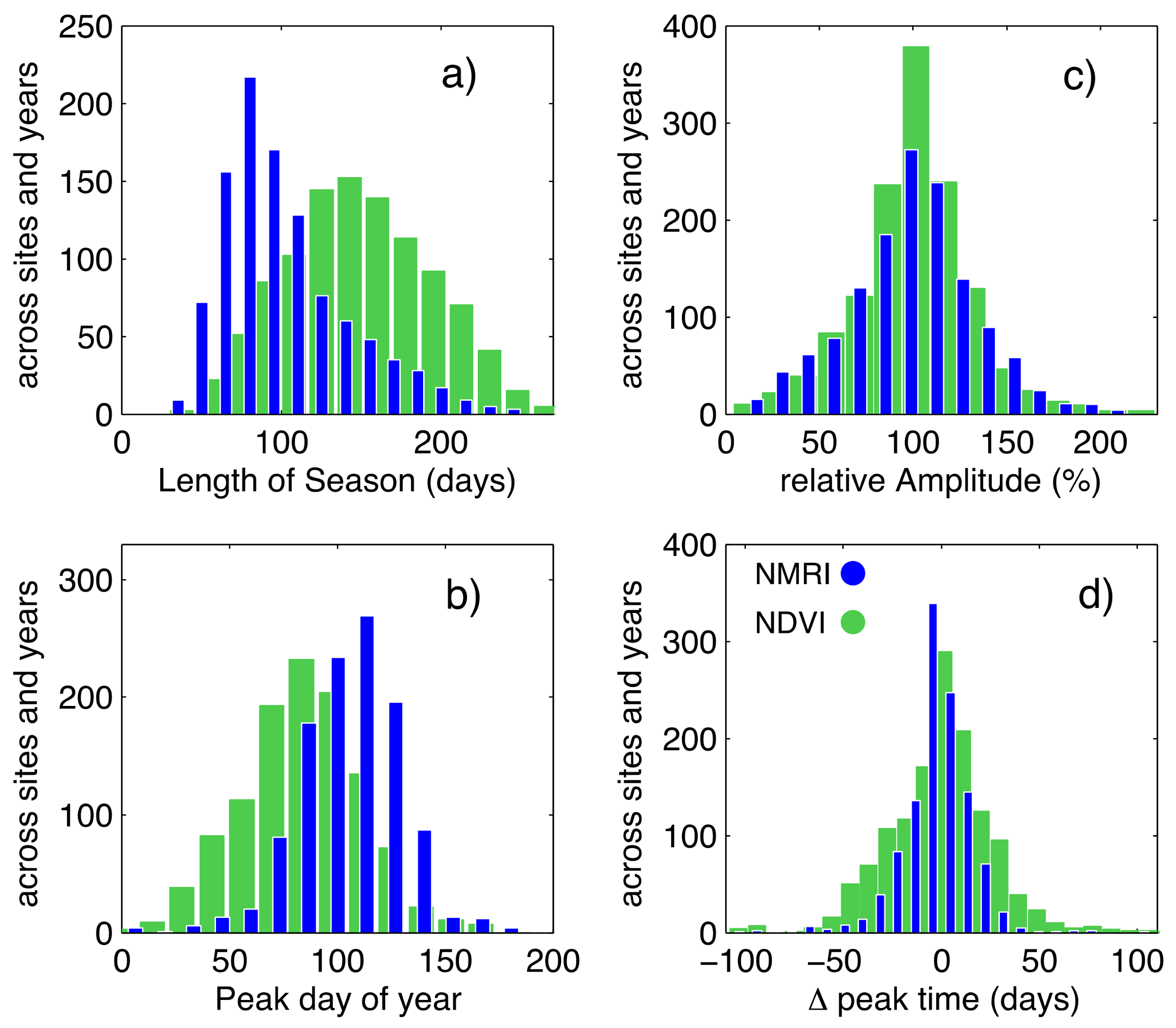
Prior to considering the response to drought, we first summarize differences and similarities between the phenology metrics calculated from NMRI and NDVI. The example data shown in Figure 2 and Figure 3 show that season length is shorter when calculated from NMRI than NDVI. Across all sites and years, NMRI season length is 45 days shorter than the NDVI season length (Figure 4a).
The day of year of peak growth is earlier for NDVI by 25 days across all of the sites and years (Figure 4b). Together, these results indicate that the seasonal increase in greenness measured by NDVI begins earlier in the spring, peaks sooner, and extends for a longer duration than the corresponding increases in vegetation water content that was sensed by NMRI. These differences are consistent with the results that are summarized by [34], as determined from stations across a broader region of the western U.S. and a five-year period. A comparison of the absolute magnitudes of NMRI and NDVI is not meaningful, as both metrics are normalized on their own scale.
We now compare the magnitude of variability in NMRI and NDVI, across all years and sites. Using the ten years of data for each site, we calculate a mean peak DOY on a site-by-site basis. Then, the deviation of the peak DOY for each growing season is calculated as compared to the mean value. Similarly, we calculate a mean amplitude for each site. The amplitude for each year is then represented as a percent of the mean amplitude at that site. Both NDVI and NMRI exhibit a near-normal distribution of variations in deviation of peak DOY. The standard deviation of peak DOY (Figure 4d) is larger for NDVI (24 days) than NMRI (17 days). Thus, the timing of peak growth based on NDVI varies more from year-to-year. In contrast, the magnitudes of year-to-year variations in amplitude of peak growth are slightly greater based on NMRI (Figure 4c): the standard deviation of NMRI is 33% as compared to 30% from NDVI. Variations in amplitude from both NDVI and NMRI are skewed towards lower values, although more so for NDVI. To summarize, the variations in timing of peak growth based on greenness are greater than based on vegetation water content, but the variations in amplitude of the growth based on water content are slightly greater or are similar in magnitude.
3.2. Link to Drought at the Site Level
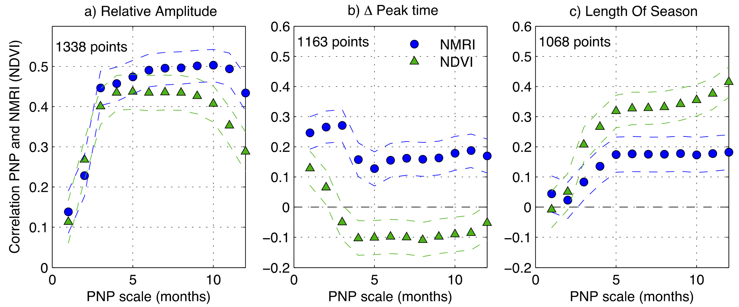
For both NMRI and NDVI, year-to-year variations in the amplitude of the seasonal growth are most strongly correlated with prior precipitation, when compared to the other phenology metrics (Figure 5). We calculated linear correlation coefficients between: (1) the year-to-year changes in each phenology metric; and, (2) deviations of precipitation prior to the growing season (PNP, Equation (1)). There is no way to know, a priori, over what time interval deviations in the magnitude of precipitation will most greatly influence vegetation. This depends on many factors, including vegetation type, climate, phenology metric, and data type analyzed. Therefore, we varied the time period for calculating precipitation anomalies between 1 and 12 months, and then calculated the correlation coefficients separately for each interval. This requires choosing a date prior to which precipitation anomalies are calculated. For each station, we chose the mean DOY of peak growth. We repeated this analysis with different dates (e.g., DOY of peak growth from individual years) and the results were nearly identical.
The amplitude of seasonal growth based on both NMRI and NDVI is positively correlated with prior normalized precipitation (PNP), with the strongest correlation being observed at intervals of 4 to 12 months (Figure 5a). This result is as expected: when precipitation is below normal prior to the growing season, the amplitude of seasonal growth is below average (and vice versa). The correlation between NMRI and PNP is slightly higher than between NDVI and PNP, particularly at timescales that are approaching one year. In Figure 6, we show how the amplitude of seasonal growth varies for different magnitudes of six-month PNP. We selected six month PNP, as this was the timescale that showed high correlations between both remote sensing indices and precipitation. NMRI Peak amplitude increases nearly linearly across the entire range of PNP observed. NDVI exhibits different behavior. When precipitation is below normal (PNP < 100%), peak amplitude increases as PNP increases. However, there is little or no relationship between peak amplitude of NDVI and PNP when the precipitation is above average. In summary, peak amplitude based on NMRI is responsive to both negative and positive precipitation anomalies, whereas NDVI peak amplitude plateaus for precipitation at (or above) normal levels.
The timing of peak growth is only weakly controlled by PNP, regardless of timescale (Figure 5b). The DOY of peak growth based on NMRI is positively correlated with PNP: peak growth tends to be earlier (later) when precipitation is below (above) normal. NDVI shows the opposite response, although the correlation is very weak: peak growth is later when precipitation is below normal. For season length, both of the indices show a positive relationship with PNP at all timescales: longer seasons for higher precipitation. The correlation between NDVI-based season length and PNP is higher than based on NMRI. The relationships between both timing of peak growth and season length are only approximately linear (not shown).
3.3. Spatial Patterns in Dry and Wet Years
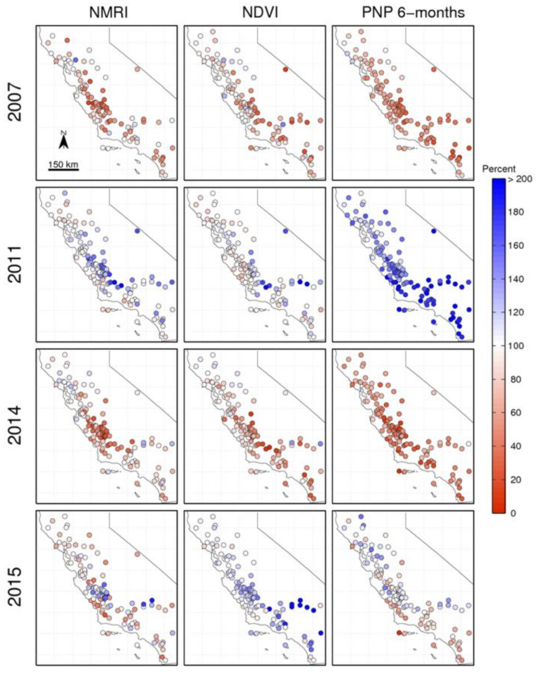
So far, this analysis has considered either all of the stations across years (Section 3.1) or all stations and their responses to variations in PNP (Section 3.2). Now, we examine the spatial patterns of precipitation and vegetation response during dry years and wet years. The maps in Figure 7 show six-month PNP and normalized peak amplitude for two dry years (2007 and 2014), a wet year (2011), and a normal year that followed the multi-year drought (2015).
For the two dry years, there is a general correspondence between the spatial patterns of precipitation and vegetation anomalies. In 2007, PNP is lowest in central California and is closer to average in the north. The vegetation response measured by NMRI peak growth is greatest in central California and decreases northward. However, NMRI peak growth exhibits some average and above-normal values in southern California that are not present in the PNP map. The pattern that is based on NDVI is similar, although near-normal peak growth is observed at even more stations where PNP is clearly below average (e.g., along the coast). In 2014, the correspondence between PNP and both of the vegetation indices is more similar, although peak growth at many stations in northern California is average or above, even though PNP is below normal.
The correspondence between the spatial patterns of precipitation and vegetation anomalies is less in the wet and normal years. This is consistent with the results presented in Figure 6: there is a weaker correlation between amplitude of growth and PNP when the precipitation is at or above average. The year 2011 was the wettest in the 10-year period examined, while 2015 was much closer to normal (Figure 7 and Figure 8). In 2011, nearly all of the sites show PNP exceeding 100%, with a south-to-north gradient from very high to nearly normal precipitation. In contrast, peak growth that is based on NDVI was close to normal everywhere, with the exception of several sites in southern California. This is expected given the complete data set (all years) that is presented in Figure 6b–NDVI anomalies and PNP are not correlated when PNP exceeds 100%. NMRI peak growth was above average at ~20 sites in central California, but close to normal otherwise. 2015 was the first year that the precipitation was near normal after three years of drought (Figure 8). Many sites in central and southern California exhibit above normal peak growth based on NDVI, even though PNP was not above average. The correlation between PNP and NMRI peak growth is higher, including the red-to-blue pattern from the coast inland observed in central California.
In summary, the correlation between PNP and peak growth from both indices is greater in dry years than wet years. More of the station-to-station differences in PNP that were observed in individual years are replicated by NMRI peak growth. NDVI peak growth shows little response to the far above-normal precipitation in 2011, consistent with the result that NDVI peak growth saturates at high values of PNP (Figure 6).
3.4. Regional-Scale Fluctuations in Precipitation and Vegetation
Finally, we consider PNP and phenology metrics that were averaged across central California (inset in Figure 1), the area with both the highest density of GPS stations and relatively strong and spatially-consistent PNP and vegetation anomalies. At the regional scale, NMRI peak amplitude tracks six-month PNP very closely (r = 0.87, p < 0.01) (Figure 8a). The correlation between NDVI peak amplitude and PNP is also high (r = 0.76, p < 0.01), although the magnitude of NDVI amplitude variations are generally less than those that are based on NMRI, which is consistent with the results that are shown above. This result demonstrates that both greenness-based and microwave-based vegetation metrics show a clear response of peak vegetation growth to precipitation anomalies at the regional scale.
The year-to-year changes in season length based on NMRI and NDVI are highly correlated, and both NMRI and NDVI season length variations are positively correlated with PNP (Figure 8b). The NDVI-based season length from 2014 is a clear outlier. The season length is almost 50 days less than observed in other years. No similar decrease was observed using NMRI. In addition, the timing of the seasonal peak was later than normal, the second highest being in the 10-year interval. We consider possible explanations for this anomalous behavior below. The year-to-year changes in timing of peak growth are similar between NMRI and NDVI. However, the correlation between either NMRI- or NDVI-based peak timing and PNP is limited or non-existent (Figure 8c).
4. Discussion
The non-forested vegetation of California shows a clear response to year-to-year fluctuations in precipitation, which is based on both microwave-based NMRI and optical-based NDVI. Of the various phenology metrics that are considered, the amplitude of seasonal vegetation growth exhibits the greatest sensitivity to prior accumulated precipitation. Above-normal precipitation from 4 to 12 months before peak growth yields a stronger seasonal pulse, and vice versa. The length of season also exhibits a positive correlation with accumulated precipitation. In contrast, variations in the timing of growth are not clearly linked to precipitation: correlations are lower and of different sign based on MNRI and NDVI. The strong, positive correlation between precipitation and amplitude of growth is consistent with numerous prior studies using ground-based and optical-remote sensing data [7]. This result is also consistent with analyses of how vegetation in water-limited ecosystems responds to variations in precipitation [45]. Of the phenology metrics that are used here, the amplitude of seasonal growth is likely to be the most robust and easiest to calculate. This could contribute to the high correlation with precipitation, when compared to the other metrics.
Overall, the microwave-based and optical-based indices exhibit similar responses to fluctuations in precipitation, yet differences do exist in terms of average season length and the timing of growth e.g., [18,34]. The most notable difference exists when the precipitation is above normal. The amplitude of seasonal growth that was determined from NDVI varies linearly with precipitation during dry years. However, it is largely insensitive to precipitation amount in years with above-normal precipitation (Figure 6). In contrast, amplitude of seasonal growth from NMRI varies approximately linearly with precipitation across the entire range of conditions observed. Peak NDVI at the sites examined here, which are primarily grassland and shrubland, is almost always below 0.6. Therefore, it is unlikely that NDVI is saturating in wet years, which typically only occurs when NDVI approaches ~0.8, as is the case for forests or crops with high leaf area index [46]. Instead, the limited sensitivity of NDVI to above-normal precipitation may indicate that greenness actually reaches an upper limit at these sites. Ecosystem productivity may still be elevated in seasons with above-normal precipitation because the vegetation tends to stay green longer in these years (Figure 5c), even if the magnitude of peak greenness is not elevated.
Both the NMRI and NDVI responses that are documented here are primarily indicative of herbaceous ground-cover and small woody shrubs, not trees. Three quarters of the sites analyzed are from grassland or shrubland (Figure 1). For the woody savanna sites, the PBO installation is typically located 10’s of m from any individual trees or areas of forest cover. The NMRI signal is dominated by the vegetation closer to the antenna [23]. Because the optical data has a larger spatial footprint, the NDVI data from these sites also integrates the effects of changes in greenness of trees. Previous studies of the vegetation response to precipitation have identified differences between passive microwave and optical responses in areas with different amounts of tree cover [18]. This type of comparison is not possible with the NMRI data used here, as NMRI data are largely sensitive to the herbaceous ground-cover and the small shrubs that surround the GPS antennas.
By using decade-long records, we can qualitatively compare the vegetation response that is associated with a multi-year drought (2012–2014) to that associated with a single dry year (2007). Precipitation in California was slightly above normal during water year 2006 (not shown), so the low precipitation observed in 2007 (Figure 8) represents a one-year event. The recovery from the one and three-year events appears to be similar. At the regional scale, the amplitude of growth increased to typical values in the first year with near-normal precipitation (2008 and 2015) (Figure 8a). The change in season length based on NDVI during the third, and most severe, year of the 2012–2014 drought is notable. PNP during 2014 was under 50%, which is very similar to that observed in 2007. However, NDVI-based season length decreased by over 50 days during 2014, which was not observed during 2007. Accumulated drought stress that is associated with the preceding dry years could explain this outlier. Alternatively, the precipitation that did occur in 2014 accumulated later in the year than normal (e.g., Figure 2), which could have resulted in the shorter growing season.
5. Conclusions
Here, we used both microwave- and optical-based observations to monitor the vegetation response to drought. We used reflected microwave signals measured by a network of ground-based GPS systems that were installed to measure crustal deformation, so the data were limited to the locations of operational GPS sites. Space-based GPS receivers can be used to monitor land surface conditions [47] providing measurements that are more spatially continuous. This type of space-based GPS reflection system could be used to monitor vegetation, providing a data stream that is complementary to the typically-used optical-based products.
Acknowledgments
PBO H2O was funded by the NSF Atmospheric Sciences, EarthScope, and Hydrological Sciences programs, most recently via AGS 1449554. NASA NNX12AK21G supported the development of GPS vegetation products. We thank John Braun, Valery Zavorotny, Clara Chew, Ethan Gutmann, Evan Pugh, Felipe Nievinski, Sarah Evans, and Jay Fein. Some of this material in this paper is based on data, equipment, and engineering services provided by UNAVCO through the GAGE Facility with support from NSF and NASA under NSF EAR-1261833. All GPS data are openly available from UNAVCO. This paper is based on data from the NSF EarthScope initiative.
Author Contributions
Eric E. Small wrote the bulk of the manuscript, Carolyn J. Roesler helped compute NMRI measurements and did the analysis, and Kristine M. Larson helped write the manuscript and wrote the NMRI analysis systems. All authors collaborated on the analysis and discussion of the data.
Conflicts of Interest
The authors declare no conflict of interest.
References
- Dai, A. Drought under global warming: A review. Wiley Interdiscip. Rev. Clim. Chang. 2011, 2, 45–65. [Google Scholar] [CrossRef]
- Asner, G.P.; Brodrick, P.G.; Anderson, C.B.; Vaughn, N.; Knapp, D.R.; Martin, R.E. Progressive forest canopy water loss during the 2012-2015 California drought. Proc. Natl. Acad. Sci. USA 2016, 113, E249–E255. [Google Scholar] [CrossRef] [PubMed]
- Evans, J.P.; Meng, X.H.; McCabe, M.F. Land surface albedo and vegetation feedbacks enhanced the millennium drought in South-East Australia. Hydrol. Earth Syst. Sci. 2017, 21, 409–422. [Google Scholar] [CrossRef]
- Ji, L.; Peters, A.J. Assessing vegetation response to drought in the northern Great Plains using vegetation and drought indices. Remote Sens. Environ. 2004, 87, 85–98. [Google Scholar] [CrossRef]
- Breshears, D.D.; Cobb, N.S.; Rich, P.M.; Price, K.P.; Allen, C.D.; Balice, R.G.; Romme, W.H.; Kastens, J.H.; Floyd, M.L.; Belnap, J.; et al. Regional vegetation die-off in response to global-change-type drought. Proc. Natl. Acad. Sci. USA 2005, 102, 15144–15148. [Google Scholar] [CrossRef] [PubMed]
- Malone, S.L.; Tulbure, M.G.; Perez-Luque, A.J.; Assal, T.J.; Bremer, L.L.; Drucker, D.P.; Hillis, V.; Varela, S.; Goulden, M.L. Drought resistance across California ecosystems: Evaluating changes in carbon dynamics using satellite imagery. Ecosphere 2016, 7, e01561. [Google Scholar] [CrossRef]
- Wang, J.; Rich, P.M.; Price, K.P. Temporal responses of NDVI to precipitation and temperature in the central Great Plains, USA. Int. J. Remote Sens. 2003, 24, 2345–2364. [Google Scholar] [CrossRef]
- Tucker, C.J.; Choudhury, B.J. Satellite remote sensing of drought conditions. Remote Sens. Environ. 1987, 23, 243–251. [Google Scholar] [CrossRef]
- Huete, A.; Didan, K.; Miura, T.; Rodriguez, E.P.; Gao, X.; Ferreira, L.G. Overview of the radiometric and biophysical performance of the MODIS vegetation indices. Remote Sens. Environ. 2002, 83, 195–213. [Google Scholar] [CrossRef]
- Chen, D.Y.; Huang, J.F.; Jackson, T.J. Vegetation water content estimation for corn and soybeans using spectral indices derived from MODIS near- and short-wave infrared bands. Remote Sens. Environ. 2005, 98, 225–236. [Google Scholar] [CrossRef]
- Gao, B.C. NDWI—A normalized difference water index for remote sensing of vegetation liquid water from space. Remote Sens. Environ. 1996, 58, 257–266. [Google Scholar] [CrossRef]
- Serrano, L.; Filella, I.; Penuelas, J. Remote sensing of biomass and yield of winter wheat under different nitrogen supplies. Crop Sci. 2000, 40, 723–731. [Google Scholar] [CrossRef]
- Ulaby, F.T.; Wilson, E.A. Microwave attenuation properties of vegetation canopies. IEEE TGRS 1985, 23, 746–753. [Google Scholar] [CrossRef]
- Jones, M.O.; Jones, L.A.; Kimball, J.S.; McDonald, K.C. Satellite passive microwave remote sensing for monitoring global land surface phenology. Remote Sens. Environ. 2011, 115, 1102–1114. [Google Scholar] [CrossRef]
- Liu, Y.Y.; de Jeu, R.A.M.; McCabe, M.F.; Evans, J.P.; van Dijk, A. Global long-term passive microwave satellite-based retrievals of vegetation optical depth. Geophys. Res. Lett. 2011, 38, L18402. [Google Scholar] [CrossRef]
- Jones, M.; Kimball, J.; Small, E.E.; Larson, K.M. Comparing Land Surface Phenology Derived from Satellite and GPS Network Microwave Remote Sensing. Int. J. Biometeorol. 2014, 58, 1305–1315. [Google Scholar] [CrossRef] [PubMed]
- Konings, A.G.; Piles, M.; Das, N.; Entekhabi, D. L-band vegetation optical depth and effective scattering albedo estimation from SMAP. Remote Sens. Environ. 2017, 198, 460–470. [Google Scholar] [CrossRef]
- Tian, F.; Brandt, M.; Liu, Y.Y.; Verger, A.; Tagesson, T.; Diouf, A.A.; Rasmussedn, K.; Mbow, C.; Wang, Y.; Fensholt, R. Remote sensing of vegetation dynamics in drylands: Evaluating vegetation optical depth (VOD) using AVHRR NDVI and in situ green biomass data over West African Sahel. Remote Sens. Environ. 2016, 177, 265–276. [Google Scholar] [CrossRef]
- Hill, M.J.; Donald, G.E.; Vickery, P.J. Relating radar backscatter to biophysical properties of temperate perennial grassland. Remote Sens. Environ. 1999, 67, 15–31. [Google Scholar] [CrossRef]
- Paloscia, S.; Macelloni, G.; Pampaloni, P.; Santi, E. The contribution of multitemporal SAR data in assessing hydrological parameters. IEEE Geosci. Remote Sens. Lett. 2004, 1, 201–205. [Google Scholar] [CrossRef]
- Kim, Y.; Jackson, T.; Bindlish, R.; Lee, H.; Hong, S. Radar Vegetation Index for Estimating the Vegetation Water Content of Rice and Soybean. IEEE Geosci. Remote Sens. Lett. 2012, 9, 564–568. [Google Scholar] [CrossRef]
- Bousbih, S.; Zribi, M.; Lili-Chabaane, Z.; Baghdadi, N.; El Hajj, M.; Gao, Q.; Mougenot, B. Potential of Sentinel-1 Radar Data for the Assessment of Soil and Cereal Cover Parameters. Sensors 2017, 17, 2617. [Google Scholar] [CrossRef] [PubMed]
- Larson, K.M.; Small, E.E. Normalized Microwave Reflection Index, I: A Vegetation Measurement Derived from GPS Data. IEEE J. Sel. Top. Appl. Earth Obs. Remote Sens. 2014, 7, 1501–1511. [Google Scholar] [CrossRef]
- Small, E.E.; Larson, K.M.W.; Smith, W. Normalized Microwave Reflection Index, II: Validation of Vegetation Water Content Estimates at Montana Grasslands. IEEE J. Sel. Top. Appl. Earth Obs. Remote Sens. 2014, 7, 1512–1521. [Google Scholar] [CrossRef]
- Larson, K.M. GPS Interferometric Reflectometry: Applications to Surface Soil Moisture, Snow Depth, and Vegetation Water Content in the Western United States. WIREs Water 2016, 3, 775–787. [Google Scholar] [CrossRef]
- He, X.; Wada, Y.; Wanders, N.; Sheffield, J. Human water management intensifies hydrological drought in California. Geophys. Res. Lett. 2017, 44, 1777–1785. [Google Scholar] [CrossRef]
- Thomas, B.F.; Famiglietti, J.S.; Landerer, F.W.; Wiese, D.N.; Molotch, N.P.; Argus, D.F. GRACE Groundwater Drought Index: Evaluation of California Central Valley groundwater drought. Remote Sens. Environ. 2017, 198, 384–392. [Google Scholar] [CrossRef]
- Berg, N.; Hall, A. Anthropogenic warming impacts on California snowpack during drought. Geophys. Res. Lett. 2017, 44, 2511–2518. [Google Scholar] [CrossRef]
- AghaKouchak, A.; Cheng, L.; Mazdiyasni, O.; Farahmand, A. Global warming and changes in risk of concurrent climate extremes: Insights from the 2014 California drought. Geophys. Res. Lett. 2014, 41, 8847–8852. [Google Scholar] [CrossRef]
- Luo, L.F.; Apps, D.; Arcand, S.; Xu, H.T.; Pan, M.; Hoerling, M. Contribution of temperature and precipitation anomalies to the California drought during 2012–2015. Geophys. Res. Lett. 2017, 44, 3184–3192. [Google Scholar] [CrossRef]
- Potter, C. Assessment of the immediate impacts of the 2013–2014 drought on ecosystems of the California central coast. West. N. Am. Nat. 2015, 75, 129–145. [Google Scholar] [CrossRef]
- Coates, A.R.; Dennison, P.E.; Roberts, D.A.; Roth, K.L. Monitoring the Impacts of Severe Drought on Southern California Chaparral Species using Hyperspectral and Thermal Infrared Imagery. Remote Sens. 2015, 7, 14276–14291. [Google Scholar] [CrossRef]
- Rao, M.; Silber-Coats, Z.; Powers, S.; Fox, L.; Ghulam, A. Mapping drought-impacted vegetation stress in California using remote sensing. GIScience Remote Sens. 2017, 54, 185–201. [Google Scholar] [CrossRef]
- Evans, S.G.; Small, E.E.; Larson, K.M. Comparison of vegetation phenology in the western United States from reflected GPS microwave signals and NDVI. Int. J. Remote Sens. 2014, 35, 2996–3017. [Google Scholar] [CrossRef]
- Schwartz, M.D.; Ahas, R.; Aasa, A. Onset of spring starting earlier across the Northern Hemisphere. Glob. Chang. Biol. 2006, 12, 343–351. [Google Scholar] [CrossRef]
- Cleland, E.E.; Chuine, I.; Menzel, A.; Mooney, H.A.; Schwartz, M.D. Shifting plant phenology in response to global change. Trends Ecol. Evol. 2007, 22, 357–365. [Google Scholar] [CrossRef] [PubMed]
- Herring, T.A.; Melbourne, T.I.; Murray, M.H.; Floyd, M.A.; Szeliga, W.M.; King, R.W.; Phillips, D.A.; Puskas, C.M.; Santillan, M.; Wang, L. Plate Boundary Observatory and related networks: GPS data analysis methods and geodetic products. Rev. Geophys. 2016, 54, 759–808. [Google Scholar] [CrossRef]
- Larson, K.M.; Small, E.E.; Gutmann, E.; Bilich, A.; Braun, J.; Zavorotny, V. Use of GPS receivers as a soil moisture network for water cycle studies. Geophys. Res. Lett. 2008, 35, L24405. [Google Scholar] [CrossRef]
- Larson, K.M.; Gutmann, E.; Zavorotny, V.; Braun, J.; Williams, M.; Nievinski, F. Can We Measure Snow Depth with GPS Receivers? Geophys. Res. Lett. 2009, 36, L17502. [Google Scholar] [CrossRef]
- Small, E.E.; Larson, K.M.; Braun, J.J. Sensing Vegetation Growth with GPS Reflection. Geophys. Res. Lett. 2010, 37, L12401. [Google Scholar] [CrossRef]
- Swets, D.L.; Reed, B.C.; Rowland, J.R.; Marko, S.E. A weighted least-squares approach to temporal smoothing of NDVI. In Proceedings of the 1999 ASPRS Annual Conference, from Image to Information, Portland, OR, USA, 17–21 May 1999. [Google Scholar]
- Xia, Y.; Mitchell, K.; Ek, M.; Sheffield, J.; Cosgrove, B.; Wood, E.; Luo, L.; Alonge, C.; Wei, H.; Meng, J.; et al. (NLDAS-2): 1. Intercomparison and application of model products. J. Geophys. Res. 2012, 117, D03109. [Google Scholar] [CrossRef]
- Daly, C.; Neilson, R.P.; Phillips, D.L. A statistical-topographic model for mapping climatological precipitation over mountainous terrain. J. Appl. Meteorol. 1994, 33, 140–158. [Google Scholar] [CrossRef]
- McKee, T.B.; Doeskin, N.J.; Kleist, J. The relationship of drought frequency and duration to time scales. In Proceedings of the 8th Conference on Applied Climatology. American Meteorological Society, Anaheim, CA, USA, 17–22 January 1993; pp. 179–184. [Google Scholar]
- Huxman, T.E.; Smith, M.D.; Fay, P.A.; Knapp, A.K.; Shaw, M.R.; Loik, M.E.; Smith, S.D.; Tissue, D.T.; Zak, J.C.; Weltzin, J.F.; et al. Convergence across biomes to a common rain-use efficiency. Nature 2004, 429, 651–654. [Google Scholar] [CrossRef] [PubMed]
- Huete, A.R.; Liu, H.Q.; van Leeuwen, W.J.D. The use of vegetation indices in forested regions: Issues of linearity and saturation. In Proceedings of the IGARSS ’97: 1997 International Geoscience and Remote Sensing Symposium: Remote Sensing—A Scientific Vision for Sustainable Development, Singapore, 3–8 August 1997; pp. 1966–1968. [Google Scholar]
- Chew, C.; Shah, R.; Zuffada, C.; Hajj, G.; Masters, D.; Mannucci, A.J. Demonstrating soil moisture remote sensing with observations from the UK TechDemoSat-1 satellite mission. Geophys. Res. Lett. 2016, 43, 3317–3324. [Google Scholar] [CrossRef]
Figure 1.
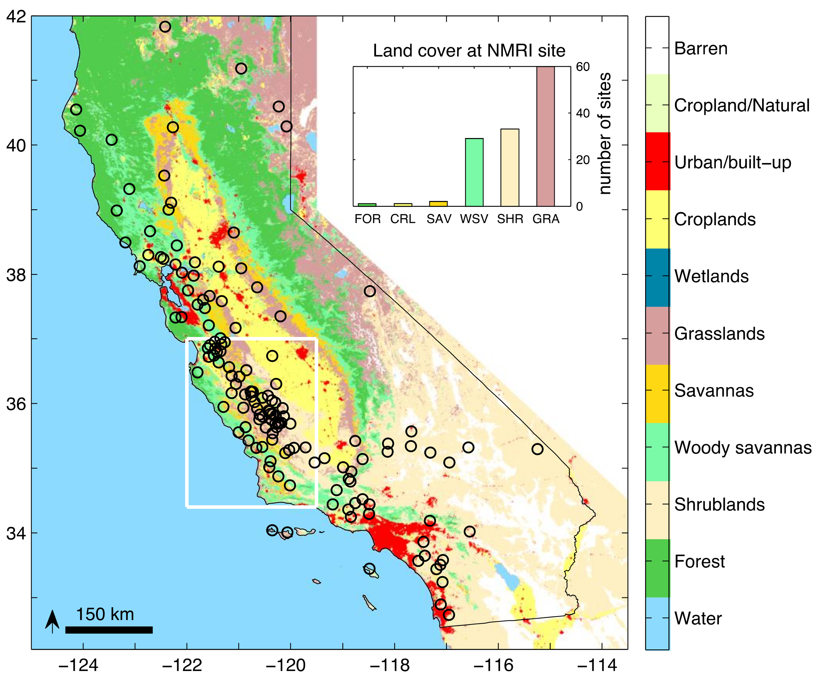
Location of the 146 GPS stations used in this study. The background represents the MODIS IGBP land cover classification. The white rectangle is the region chosen for the regional-average analysis. The inset shows the number of Normalized Microwave Reflection Index (NMRI) sites by land cover type (GRA grassland, SHR shrubland, WSV woody savanna, SAV savanna, CRP cropland, FOR forest).
Figure 1.
Location of the 146 GPS stations used in this study. The background represents the MODIS IGBP land cover classification. The white rectangle is the region chosen for the regional-average analysis. The inset shows the number of Normalized Microwave Reflection Index (NMRI) sites by land cover type (GRA grassland, SHR shrubland, WSV woody savanna, SAV savanna, CRP cropland, FOR forest).

Figure 2.
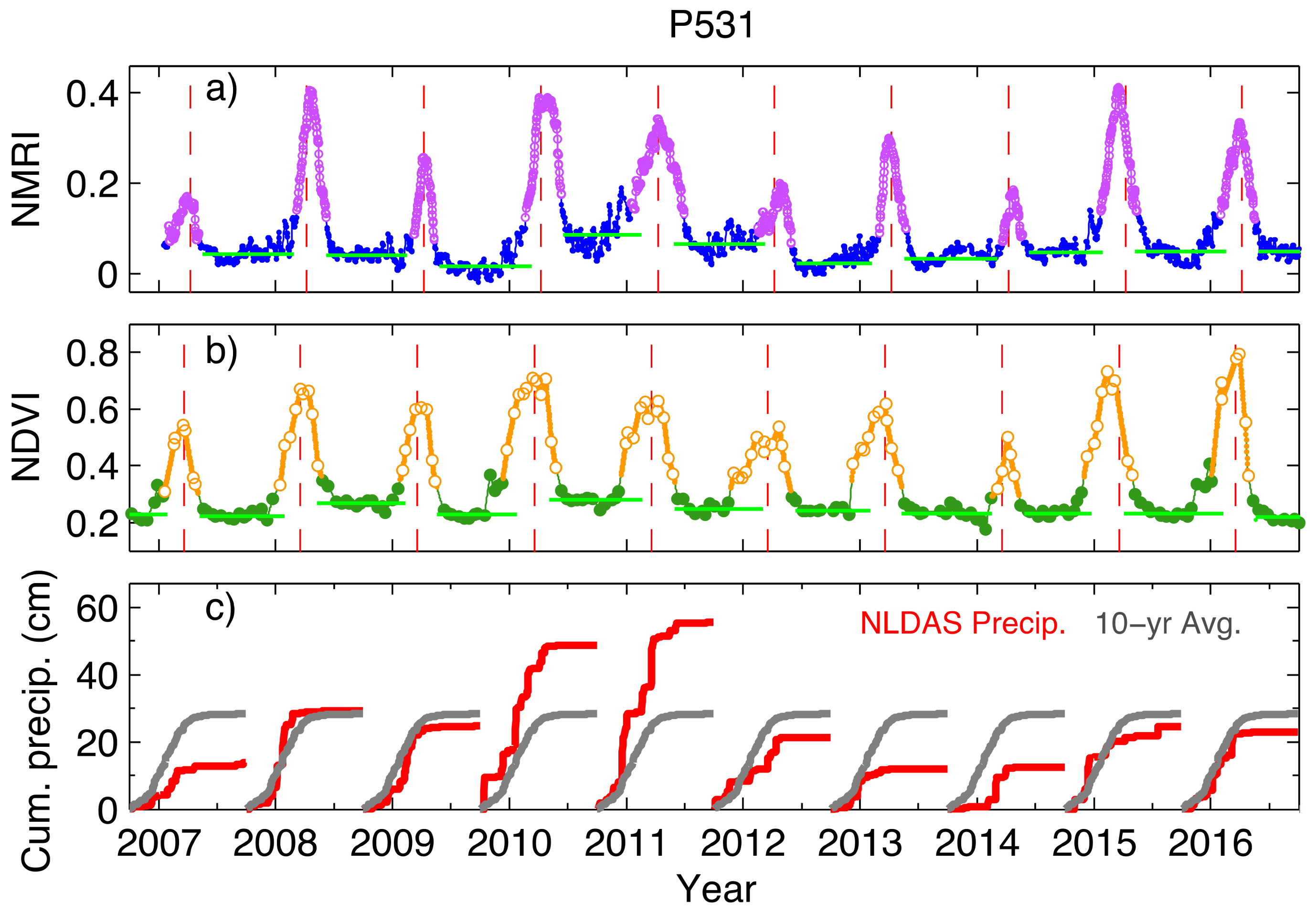
Time series for GPS site P531: (a) NMRI time series after application of a five-day centered median filter; (b) Normalized Difference Vegetation Index (NDVI) data including linear interpolation between observed values. (a,b) data analysis: Green horizontal lines show the baseline level for amplitude calculation, determined separately between peaks. The lavender (yellow) circles for NMRI (NDVI) show the interval above the 25% cut-off around the main seasonal peak. The red vertical dashed line is the Mean Peak day of year. (c) North American Land Data Assimilation System (NLDAS) cumulative precipitation for each Water Year (red), and the 10-year average (gray). P531 is a grasslands site with an annual precipitation of 428 mm at latitude/longitude of N 35.8° and W 120.54°.
Figure 2.
Time series for GPS site P531: (a) NMRI time series after application of a five-day centered median filter; (b) Normalized Difference Vegetation Index (NDVI) data including linear interpolation between observed values. (a,b) data analysis: Green horizontal lines show the baseline level for amplitude calculation, determined separately between peaks. The lavender (yellow) circles for NMRI (NDVI) show the interval above the 25% cut-off around the main seasonal peak. The red vertical dashed line is the Mean Peak day of year. (c) North American Land Data Assimilation System (NLDAS) cumulative precipitation for each Water Year (red), and the 10-year average (gray). P531 is a grasslands site with an annual precipitation of 428 mm at latitude/longitude of N 35.8° and W 120.54°.

Figure 3.
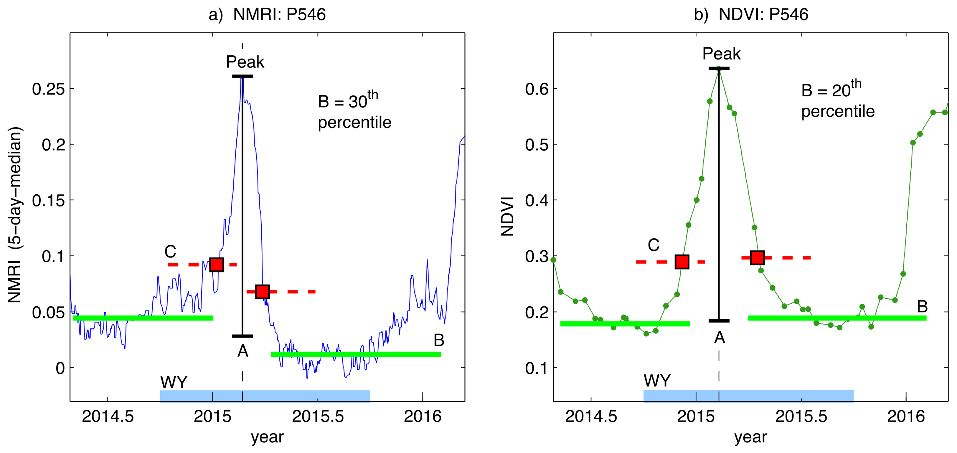
Example analysis used to retrieve the amplitude of the seasonal peak, the Start of Season (SOS) and End of Season (EOS) day of year. The seasonal peak is within the Water Year (thick light blue line on x-axis labeled WY). The baseline (green line B) on each side of the peak is the level of pre/post-growth vegetation. The amplitude (black line A) is the difference between the peak and the average baseline pre/post-growth. The red dotted lines are the 25% cut off levels with respect to the pre/post-growth baselines, and they intersect the main seasonal growth cycle at the SOS and EOS day of year (red squares). (a) the daily five-day median NMRI uses the 30th percentile to define the baseline; and, (b) the interpolated bi-weekly NDVI uses the 20th percentile.
Figure 3.
Example analysis used to retrieve the amplitude of the seasonal peak, the Start of Season (SOS) and End of Season (EOS) day of year. The seasonal peak is within the Water Year (thick light blue line on x-axis labeled WY). The baseline (green line B) on each side of the peak is the level of pre/post-growth vegetation. The amplitude (black line A) is the difference between the peak and the average baseline pre/post-growth. The red dotted lines are the 25% cut off levels with respect to the pre/post-growth baselines, and they intersect the main seasonal growth cycle at the SOS and EOS day of year (red squares). (a) the daily five-day median NMRI uses the 30th percentile to define the baseline; and, (b) the interpolated bi-weekly NDVI uses the 20th percentile.

Figure 4.
Histograms of (a) Length of season; (b) Mean peak day of year; (c) Relative amplitude; and, (d) Deviation from the mean peak day of year. Histograms are for all sites over all years.
Figure 4.
Histograms of (a) Length of season; (b) Mean peak day of year; (c) Relative amplitude; and, (d) Deviation from the mean peak day of year. Histograms are for all sites over all years.

Figure 5.
Correlation between the Percent of Normal Precipitation (PNP) computed for the month prior to the NMRI mean seasonal peak day of year (DOY) and NMRI metrics as a function of the PNP scale in months (blue circles). (a) Relative Amplitude; (b) Deviation from the Mean Peak DOY; and, (c) Length of Season. The dashed lines are the 95% confidence interval. The green triangles are the correlation results using NDVI, with PNP computed for the month prior to the NDVI mean seasonal peak.

Figure 6.
NMRI (a) and NDVI (b) relative amplitude (small dots) versus the corresponding 6-month Percent of Normal Precipitation (PNP). The large symbols are the averaged values over 40% wide PNP bins incremented every 20%. Each bin has a number of points >50.
Figure 6.
NMRI (a) and NDVI (b) relative amplitude (small dots) versus the corresponding 6-month Percent of Normal Precipitation (PNP). The large symbols are the averaged values over 40% wide PNP bins incremented every 20%. Each bin has a number of points >50.

Figure 7.
NMRI (left) and NDVI (middle) relative peak amplitude for Plate Boundary Observatory (PBO) H2O sites in California, during two dry years (2007 and 2014), a wet year (2011), and a normal year (2015) following a multi-year drought; (Right) six-month Percent of Normal Precipitation (PNP). Both vegetation metrics and PNP are compared to the average for 2007–2016 and reported as a percentage, as shown in the color bar.

Figure 8.
Central California averaged (inset Figure 1, 55 sites) phenology metrics and one standard deviation as a function of year during 2007–2016, using NDVI (green triangles) and NMRI (blue circles); (a) Relative Amplitude; (b) Length of Season; and, (c) Deviation in time of peak growth. The averaged PNP is displayed in all plots (pink squares), with one standard deviation shown only in (a).

© 2018 by the authors. Licensee MDPI, Basel, Switzerland. This article is an open access article distributed under the terms and conditions of the Creative Commons Attribution (CC BY) license (http://creativecommons.org/licenses/by/4.0/).
Share and Cite
MDPI and ACS Style
Small, E.E.; Roesler, C.J.; Larson, K.M. Vegetation Response to the 2012–2014 California Drought from GPS and Optical Measurements. Remote Sens. 2018, 10, 630. https://doi.org/10.3390/rs10040630
AMA Style
Small EE, Roesler CJ, Larson KM. Vegetation Response to the 2012–2014 California Drought from GPS and Optical Measurements. Remote Sensing. 2018; 10(4):630. https://doi.org/10.3390/rs10040630
Chicago/Turabian StyleSmall, Eric E., Carolyn J. Roesler, and Kristine M. Larson. 2018. "Vegetation Response to the 2012–2014 California Drought from GPS and Optical Measurements" Remote Sensing 10, no. 4: 630. https://doi.org/10.3390/rs10040630
Note that from the first issue of 2016, this journal uses article numbers instead of page numbers. See further details here.