Icing Detection over East Asia from Geostationary Satellite Data Using Machine Learning Approaches


1
School of Urban and Environmental Engineering, Ulsan National Institute of Science and Technology, Ulsan 44919, Korea
2
Department of Climate and Energy Systems Engineering, Ewha Woman’s University, Seoul 03760, Korea
3
Hong Kong Observatory, 134A Nathan Road, Kowloon, Hong Kong, China
*
Author to whom correspondence should be addressed.
Remote Sens. 2018, 10(4), 631; https://doi.org/10.3390/rs10040631
Submission received: 13 March 2018
/
Revised: 10 April 2018
/
Accepted: 17 April 2018
/
Published: 19 April 2018
(This article belongs to the Special Issue Remote Sensing Methods and Applications for Traffic Meteorology)
Abstract
:Even though deicing or airframe coating technologies continue to develop, aircraft icing is still one of the critical threats to aviation. While the detection of potential icing clouds has been conducted using geostationary satellite data in the US and Europe, there is not yet a robust model that detects potential icing areas in East Asia. In this study, we proposed machine-learning-based icing detection models using data from two geostationary satellites—the Communication, Ocean, and Meteorological Satellite (COMS) Meteorological Imager (MI) and the Himawari-8 Advanced Himawari Imager (AHI)—over Northeast Asia. Two machine learning techniques—random forest (RF) and multinomial log-linear (MLL) models—were evaluated with quality-controlled pilot reports (PIREPs) as the reference data. The machine-learning-based models were compared to the existing models through five-fold cross-validation. The RF model for COMS MI produced the best performance, resulting in a mean probability of detection (POD) of 81.8%, a mean overall accuracy (OA) of 82.1%, and mean true skill statistics (TSS) of 64.0%. One of the existing models, flight icing threat (FIT), produced relatively poor performance, providing a mean POD of 36.4%, a mean OA of 61.0, and a mean TSS of 9.7%. The Himawari-8 based models also produced performance comparable to the COMS models. However, it should be noted that very limited PIREP reference data were available especially for the Himawari-8 models, which requires further evaluation in the future with more reference data. The spatio-temporal patterns of the icing areas detected using the developed models were also visually examined using time-series satellite data.
1. Introduction
Aircraft icing is a dangerous threat that results in many accidents which can cause fatalities and financial losses [1,2]. It is a phenomenon in which supercooled droplets (SCDs) collide with a hard surface forming an ice film. Clouds often contain SCDs, but icing occurs when there is a high density of SCDs [3,4,5]. When icing forms on aircraft bodies and wings, the aircraft’s balance is disturbed, resulting in a loss of control. For this reason, detecting and avoiding potential icing areas is crucial for aviation safety. The detection of SCDs, especially in the freezing phase of rain, is usually conducted using a thresholding approach based on the subfreezing temperature range and high relative humidity [6].
Research efforts have been made to identify icing regions using ground or airborne observations and human reporting systems such as Tropospheric Airborne Meteorological Data Reporting (TAMDAR) and pilot reports (PIREPs). Such systems are designed to warn other flights by recording the time and location with detailed atmospheric information when airplanes are crossing dangerous areas [7]. Although observation data only provide limited spatiotemporal information on icing, they have been used as validation data in many icing-related studies [8,9,10].
Numerical forecasting models have also been used to estimate potential icing regions. For instance, high resolution numerical weather prediction model results have been used to calculate temperature (T), relative humidity (RH), vertical velocity (VV), and supercooled liquid water (SLW) as input parameters in potential icing calculation algorithms [10,11]. However, numerical models often provide inaccurate results [12], which increase the uncertainty of potential icing clouds identified by the icing algorithms [13].
Geostationary satellite sensors can be an effective alternative because they collect data over wide areas with high temporal frequency (~minutes). SLW, which potentially results in icing, tends to form near cloud tops where the air temperatures typically range from freezing temperature to −30 °C [14]. Thus, satellite observations over cloud tops can provide valuable information on icing [15]. In particular, satellite-derived data are greatly suitable for icing research due to the fact that icing intensity is closely related to several meteorological factors such as cloud temperature, thickness, phase, and distribution, which can be effectively derived from satellite images [15,16,17].
With an increasing interest in the synergistic use of satellite and ground observations for icing detection, many agencies and research groups have developed operational systems for icing detection, including the Flight Icing Threat (FIT) [15], and the National Aeronautics and Space Administration (NASA) Icing Remote Sensing System (NIRSS) [18]. The Alliance Icing Research Study (AIRS) investigated the climatological characteristics of icing with varying intensities over Canada, and compared meteorological data between aircraft measurements and ground-based remote sensing data, such as doppler radar, aircraft weather radar, light detection and ranging (LIDAR), infra-red (IR) and visible sensors [19]. The IR brightness temperature data derived from advanced very high resolution radiometers (AVHRR) onboard the National Oceanic and Atmospheric Administration (NOAA) polar-orbiting satellites were used for icing detection with temperature and relative humidity (T/RH) derived from numerical models, which resulted in a probability of detection (POD) of up to 70% for moderate-or-greater icing [17]. Minnis et al. [16] examined the feasibility of the cloud parameters produced from Geostationary Operational Environmental Satellite (GOES) satellite data as input factors in an icing detection algorithm. They suggested a probability-based algorithm with an empirical equation focusing on the liquid water path (LWP) and evaluated it with PIREPs resulting in a POD of 54.5%.
Bernstein et al. [10] proposed an icing detection algorithm that uses cloud effective radius (CER), cloud optical thickness (COT), and LWP products generated from GOES satellite data. The algorithm was based on a thresholding approach where the thresholds were determined through statistical analyses using a huge amount of in situ data over the contiguous United States (CONUS) region. They combined a fuzzy logic membership function and a human-derived decision tree to determine the thresholds rather than using simple physical thresholds such as those used in the T/RH scheme. The proposed icing detection algorithm was successfully validated using four hindcast icing cases. Smith et al. [15] improved the icing detection model proposed by Bernstein et al. [10], suggesting an operational NOAA FIT algorithm. However, the algorithm produced a high false alarm rate in detecting potential icing areas due to the different scales between satellite and reference data, because icing often occurs in a smaller region than the pixel size (i.e., 4 km by 4 km) of the satellite data used [15]. The thresholding approach based on the physical characteristics of icing has some limitations. Above all, the determination of thresholds for meteorological factors tends to be subjective, depending on experts [20]. Moreover, several factors in a physical icing algorithm come from model outputs (e.g., T, RH, and VV), which implies that the algorithm strongly depends on the accuracy of the corresponding physical model [10].
Although many studies have been conducted to detect and monitor satellite-based flight icing [15,21], they have focused on the areas over North America and Europe. There has been minimal exploration of satellite-based flight icing detection in Asia, even though several meteorological satellite sensor systems are in operation, such as the Communication, Ocean and Meteorological Satellite (COMS) Meteorological Imager (MI) and the Himawari-8 Advanced Himawari Imager (AMI). The Korea Meteorological Administration (KMA) proposed an icing detection system using COMS MI over East Asia [22]. The KMA algorithm produced a high false alarm rate when compared to PIREPs because it is a composite model of thresholding approaches based solely on the physical theory of icing [22]. This implies that the physical properties of in-flight potential icing regions might vary by location and adaptive thresholding approaches may need to be considered in order for a model to work with different areas and data.
A robust icing detection model can be proposed using a number of reference data for calibration and validation. Thus, it is necessary to evaluate icing detection models using long term data covering more than a few years, unlike the existing studies which have mostly focused on the evaluation of a short period of time (e.g., a few months or specific seasons) [10,15,16,17,19,22].
Although several satellite-derived variables such as COT and CER are related to icing, each variable has its own uncertainty and the relationship between the variables and icing might not be robustly determined through a simple thresholding approach, which implies that more advanced approaches capable of handling non-linear behaviors are necessary for icing detection.
Recently, machine learning approaches have been introduced in many classification and regression tasks using satellite remote sensing [23,24,25,26,27,28]. Unlike typical statistical approaches, machine learning is generally free from data assumptions and has been proven to be effective in modeling non-linear behaviors. For meteorological applications, machine learning has been applied to detect phenomena that pose a risk to aviation, such as overshooting tops and cloud convective initiation [29,30,31].
The objectives of this research were to (1) develop icing detection algorithms for a portion of East Asia based on machine learning approaches with COMS MI and Himawari-8 AHI products; (2) compare the proposed algorithms with the existing FIT and KMA algorithms; and (3) interpret the properties of the potential icing clouds identified by the algorithms. Two machine learning approaches—random forest (RF) and multinomial log-linear model (MLL)—were used in this study.
2. Study Area and Data
2.1. Study Area
A part of East Asia was selected as the study area based on the spatial extent of the obtained reference data (i.e., PIREPs). The area (i.e., 94–141° E and 5–47° N) covers the major countries of East Asia (i.e., the Korean Peninsula, Japan, China, Hong Kong, and Taiwan). Based on the total air passenger traffic in 2016, one quarter of the world’s top 20 airports are located in this region [32].
2.2. Geostationary Satellite Data
COMS is Korea’s first multi-purpose geostationary satellite, and is equipped with a Meteorological Imager (MI) sensor observing East Asia every 15 min [33]. COMS MI provides data at one visible, shortwave infrared (SWIR), water vapor (WV), and two IR channels [22,29] (Table 1). COMS MI also provides level 2 products such as cloud analysis (CA) and cloud top temperature and heights (CTTP), which quantify the inner and upper properties of clouds. CA contains COT, measuring the optical depth of clouds with a scaling from 0 to 100; and cloud phase (CP), providing information on whether the major portion of a near cloud top is water, ice, mixed, unknown, or if the sky is clear [33,34,35]. CTTP provides information on cloud top conditions, including cloud top temperature (CTT), cloud top height (CTH), and cloud top pressure (CTP) [33,34,35]. The spatial resolution of the visible channel is 1 km, while the other products have a resolution of 4 km. COMS MI products were downloaded through the National Meteorological Satellite Center (NMSC) webpage (http://nmsc.kma.go.kr/).
Himawari-8, a replacement of the Japanese Multifunctional Transport Satellite 2 (MTSAT-2), was launched by Japan Meteorological Agency (JMA) on 7 October 2014. Its major instrument is the Advanced Himawari Imager (AHI) that has 16 bands with a high spatial resolution (500 m–2 km), and scans Northeast Asia every 10 min [36,37,38]. The bands consist of three visible channels with 0.5–1 km resolution and thirteen IR channels with 1–2 km resolution (Table 1). In this study, we used only 14 bands from the site (ftp://hmwr829gr.cr.chiba-u.ac.jp/) because there are not yet publicly available cloud products from Himawari-8. COMS data from April 2011 to July 2017 and Himawari-8 data from July 2015 to July 2017 were used in this study.
2.3. Pilot Reports
Most aero-vehicles provide specific flight logs created by the pilot when they fly through areas of potentially problematic conditions or pre-defined areas. They record the time, position, and external environmental conditions that may cause aviation problems. Such flight logs are called PIREPs. These records provide information on not only basic external conditions (e.g., temperature, wind direction, and wind speed) but also particular events (e.g., turbulence and accretion of ice on the airframe) with the time and location. When ice crystals form on the aircraft body, it is recorded as ‘icing’ on the PIREP, together with its severity; this has been commonly used as reference data to develop and validate icing detection algorithms [10,14,39]. PIREPs are accumulated extensively in the CONUS, with thousands of icing records per year [10,15]. However, unlike the US, a relatively small number of icing observations are reported in East Asia. In this study, PIREPs from KMA and the Hong Kong Observatory (HKO) were used as reference data to develop icing detection algorithms.
Although PIREPs are commonly used as reference data for icing research, they are subjective and thus might provide inaccurate icing information. Furthermore, some PIREPs are reported in a few specific locations designated by governmental agencies. Thus, a quality control (QC) process for PIREPs should be conducted before using them as reference data. QC consists of several rules to verify that an icing PIREP has been obtained in an area corresponding to the physical characteristics of potential icing (e.g., SLW clouds). Table 2 shows the rules used to conduct the quality control of PIREPs using flight information and satellite-derived products. While a total of 54 icing PIREP cases (36 from HKO and 18 from KMA) were originally collected for COMS applications, only 24 PIREP cases were available for Himawari-8 applications. Through quality control, a total of 48 and 20 icing PIREPs were selected to develop icing detection models for COMS and Himawari applications, respectively. In addition, 113 carefully selected non-icing references from KMA PIREPs were used to develop the icing models (Table 3).
3. Methodology
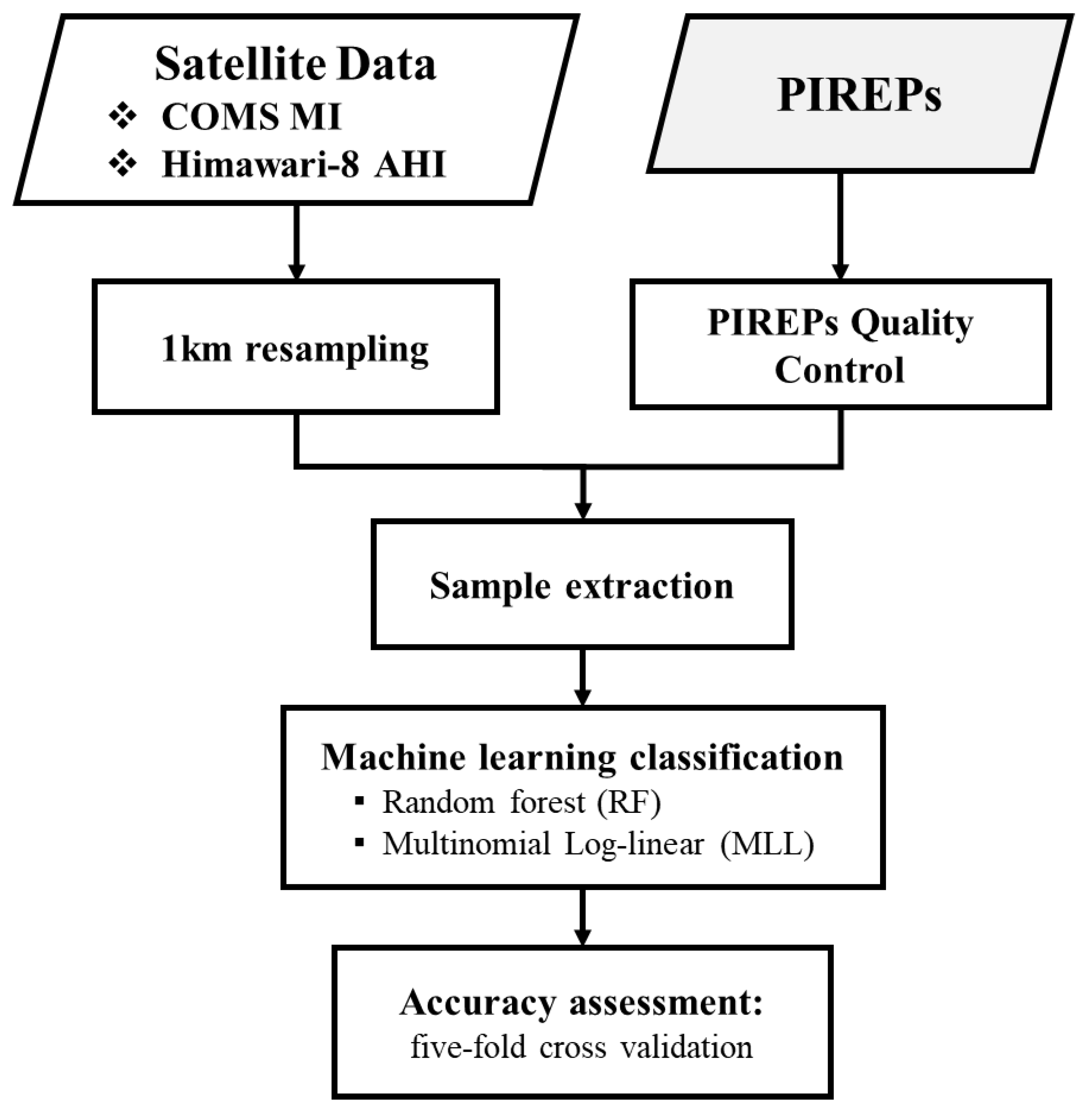
A flow chart of the proposed approach is provided in Figure 1. COMS MI and Himawari-8 AHI products were used as the input data. Since the satellite data have different spatial resolutions, all data were resampled to 1 km before input features were extracted based on the PIREP data. The extracted samples were used to develop icing detection models and a five-fold cross-validation method was used to evaluate the proposed models.
3.1. Sample Extraction
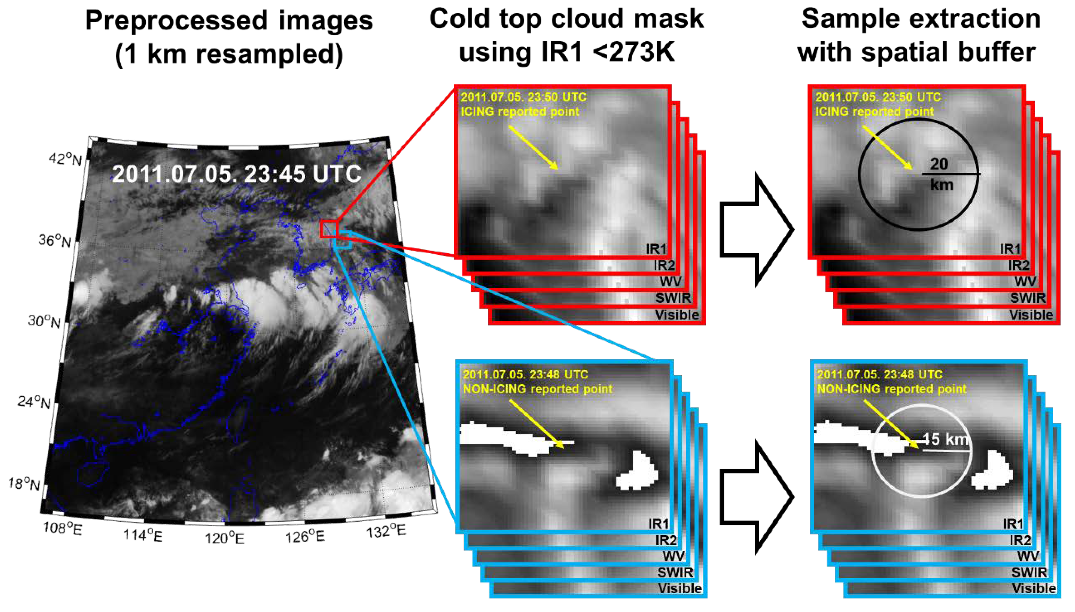
Since PIREPs are point-based data, spatial samples should be extracted to develop empirical icing detection models. In this study, a sample extraction method was used to obtain icing and non-icing samples from the COMS and Himawari-8 data. Once resampling of the input data was conducted, icing and non-icing samples were extracted using a cold cloud top temperature mask and spatial buffering (Figure 2). The cold cloud top mask uses the IR1 channel from COMS, and CH13 from Himawari-8 with a threshold of 273 K brightness temperature, since IR1 and CH13 (i.e., ~11 µm) represent cloud top temperature [3,40]. Since point-based icing PIREP data typically have a spatial significance of ~20 km in radius [10], a buffer with a radius of 20 km from an icing PIREP location was used to extract the icing pixels in this study. For non-icing samples, a more conservative buffer size (i.e., a radius of 15 km) was used to ensure the reliability of the training data, as much more non-icing PIREP data exists compared to icing PIREP data.
Through these processes, a total of 53,760 icing and 117,148 non-icing pixels for COMS, and 5506 icing and 12,352 non-icing pixels for Himawari-8, respectively, were extracted as reference data. The reference data were divided into five groups based on icing and non-icing cases, not individual pixels, and a five-fold cross validation was conducted to evaluate the machine-learning-based icing detection models.
3.2. Machine Learning
Random forest (RF) has proven very effective for several meteorological satellite-based applications such as the detection of convective initiation and overshooting tops, and rainfall rate estimation [29,30,31,41]. The multinomial log-linear model (MLL) is an improved version of logistic regression that incorporates an artificial neural network approach for parameter optimization [42]. Logistic regression has often been used in meteorological satellite applications [30,31] and operational systems, such as to monitor rapid development thunderstorms (RDT) using Spinning Enhanced Visible and Infrared Imager (SEVIRI) satellite data [43]. Thus, in this study, the two machine learning classification approaches—RF and MLL via neural networks—were used to develop icing detection models. RF, which is based on classification and regression trees (CART; [44]), produces numerous CARTs and adopts an ensemble approach to obtain the final output from the resultant trees. It incorporates two randomizations to overcome the major limitation of CART, which is the sensitivity to training data configuration, which often results in overfitting. By developing many independent trees from different sets of training samples and input variables, RF tries to provide relatively unbiased results [45,46,47]. RF has proven useful in various remote sensing tasks for both classification and regression [48,49,50,51]. RF also provides information on how input variables contribute to a given task. It calculates the decrease in accuracy using out-of-bag samples when an input variable is perturbed [52,53,54]. The larger the decrease in accuracy, the more significant the variable. RF can provide results in probability form from the ensemble approach.
MLL is a type of linear classification model for predicting the logarithmic form of a dependent variable [55,56]. MLL can be calculated by Equation (1):
where y is the instant target variable, i is each input variable, ω is the weight of each variable, and the ƒ(X) is the value of each variable [55,56,57]. MLL works well when a dependent variable has complex relations with the input variables. The coefficients associated with input variables are determined through an advanced coefficient fitting approach, named neural networks. Since the coefficients of the normalized regression model imply the relative contribution of the input variables, they can be used to analyze the relative importance of the variables. In this study, MLL is implemented using an ‘nnet’ package in R, which builds a feed-forward single-hidden-layer neural network to fit MLL [57].
3.3. Existing Satellite-Based Icing Detection Algorithms
In the US, the FIT algorithm is used to identify potential icing clouds based on the physical properties of the icing [15,58]. The FIT algorithm consists of condition-based rules using CP and COT to produce a binary icing mask (Table 4). KMA also proposed an icing detection system using COMS MI products over the Northeast Asia region based on the physical characteristics of icing [22]. Similar to the FIT algorithm, the KMA algorithm consists of condition-based rules based on level-1b data and their differences (BTD) (Table 4).
3.4. Accuracy Assessment
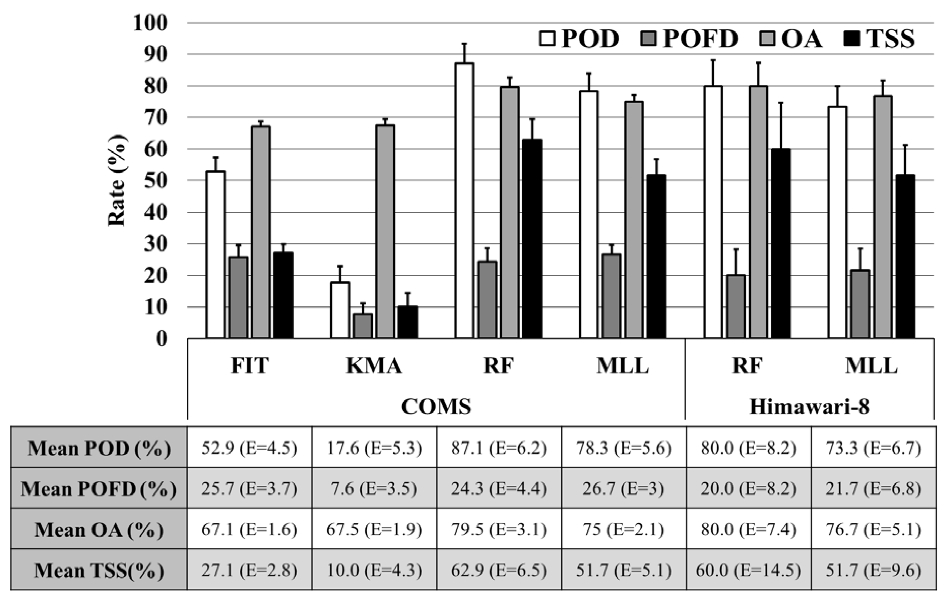
The performance of icing detection algorithms was evaluated using five-fold cross-validation based on a 2 × 2 contingency table, helping to quantify the detection probability of models [29,30,31,59,60,61] (Table 5). Based on the components of the contingency table, four performance metrics were calculated: the probability of detection (POD; calculated as H/(H + M) × 100%); the probability of false detection (POFD; calculated as F/(N + F) × 100%); overall accuracy (OA; calculated as (N + H)/(N + F+ M + H) × 100%); and total skill statistics (TSS; calculated as (H × N−F × M)/[(H + M) × (F + N)]). In addition to the performance indices, the standard error (E), which is the standard deviation divided by the total fold number, was also used to compare model stability.
4. Results and Discussion
4.1. Variable Importance
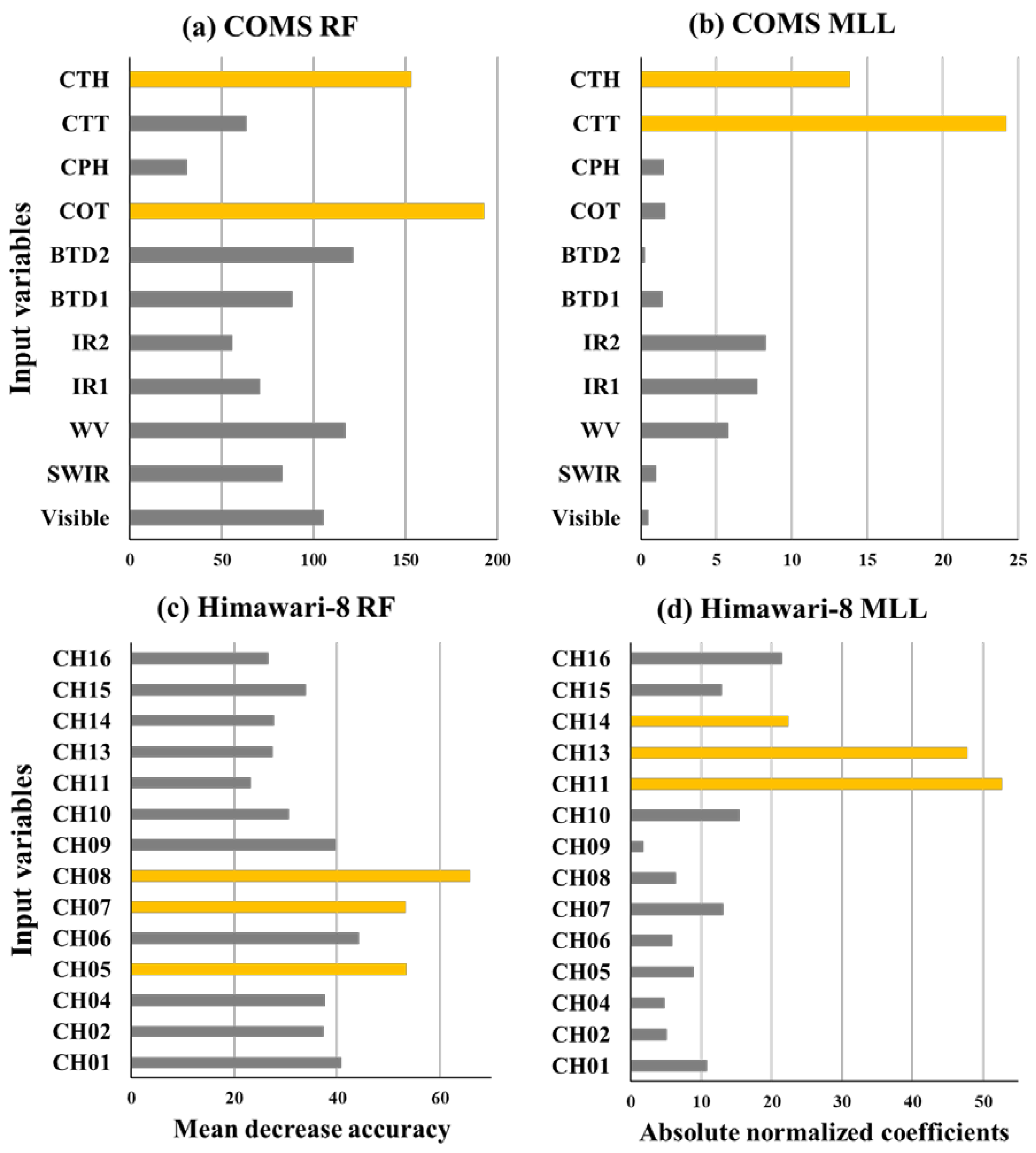
The relative variable importance identified by the RF and MLL models is shown in Figure 3. The mean decrease accuracy (MDA) values calculated when a variable is randomly permuted were used to identify significant variables in the RF model, while the absolute normalized coefficient values were used in the MLL model [62,63]. It should be noted that these metrics suggest the relative importance of variables in estimating the target variable, not the absolute indicator of variable significance.
In COMS models, while CTH was identified as being very significant for both the RF and MLL models, visible, IR2, COT, and CTT were given different relative importances from model to model (Figure 3a,b). According to the cloud product retrieval algorithm of COMS, CTH is produced using CTT and IR channels, and COT is retrieved from the visible channel [34]. Thus, the significant input variables in the COMS models can be grouped into two groups—a long-wave infrared (LWIR) group (i.e., CTH, CTT, and IR) and a visible (VIS) group (COT and visible)—which have been frequently used in icing studies [10,15,20]. While the LWIR and VIS groups are generally identified as important by RF, the LWIR group was only considered significant by the MLL models. This might be due to the skewed distribution of the variables from the VIS group. Visible-based variables are sensitive to thin clouds, but they tend to saturate with thicker clouds [34]. Thus, it is not necessary to have high coefficients for the normalized variables (i.e., sensitive to much smaller values in the range of 0–1) in the MLL model.
The variable importance given by the Himawari-8 models is somewhat different to that of the COMS models. Near-infrared (NIR) channels (i.e., CH05, CH07, and CH08) identified as the most significant variables by the RF model, while the LWIR channels (i.e., CH11, CH13, and CH14) were considered very important in the MLL model. NIR channels are widely used as a source to produce CP and cloud particle size data [33,34,35,64,65,66,67], and LWIR channels are related to the cloud top temperature and the amount of water vapor, which are the important input variables of the FIT algorithm [15].
4.2. Model Performance
The RF- and MLL-based icing detection models were developed using PIREP-based reference data for COMS and Himawari-8. Since the existing FIT and KMA models require level 2 products to generate icing masks, they were tested only with COMS data. Figure 4 shows the accuracy assessment results for the two theoretical (i.e., existing) models and the four machine learning models. When the COMS data were used, the RF model yielded the highest POD (~87.1%), OA (~79.5%), and TSS (~62.9%) among the four tested models, followed by the MLL model. However, the RF model resulted in a relatively high POFD (~24.3%) compared to the KMA model (7.6%). The standard errors of the accuracy metrics (i.e., POD, OA, and TSS) of the RF model were slightly higher than those of the MLL model, which implies that MLL showed more consistent performance than RF for icing detection. This might be due to the small number of samples for RF, resulting in slight overfitting for some folds. On the other hand, the rule-based models (i.e., FIT and KMA) consistently performed worse than the RF and MLL models, resulting in low standard errors (average ~3.5% indicating stable performance by fold) with OAs of 67.1% and 67.5%, and TSSs of 27.1% and 10.0%, respectively. Overall, the RF icing detection model resulted in the best performance among the four models for COMS.
When the Himawari-8 data were used, the results were similar to the COMS-based models; the RF model produced better performance than the MLL model. However, the accuracy difference between the RF and MLL models for Himawari-8 was smaller than that for COMS. The standard errors of the performance metrics for the Himawari-8 models were much higher than those for COMS-based models (Figure 4). For example, the standard errors of the mean TSS for the machine-learning-based COMS models were 6.5% and 5.1% (i.e., for the RF and MLL models, respectively), while those for the Himawari-8 models were 14.5% and 9.6%. Such differences in the standard errors are possibly due to the much smaller number of samples for Himawari-8 than COMS. This implies that the RF and MLL models for Himawari-8 might not be robust, often resulting in varied performance for the samples even though they produced high accuracy.
It is not appropriate to directly compare these results to those from other studies as different data were used. However, the accuracy metrics from the proposed approaches are higher than those from the literature. For example, Choi et al. [22] evaluated the KMA model using COMS–PIREP data, resulting in a POD of 57.9%, a POFD of 27.5%, an OA of 72.46%, and a TSS of 30.4%. Similarly, the FIT model was evaluated using GOES–PIREP data, yielding a POD of 62%, a POFD of 39%, an OA of 58%, and a TSS of 4% in the daytime [15]. PIREPs were used as reference data in both studies.
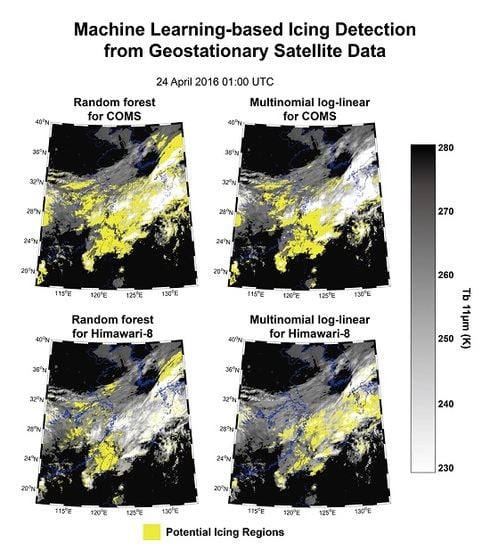
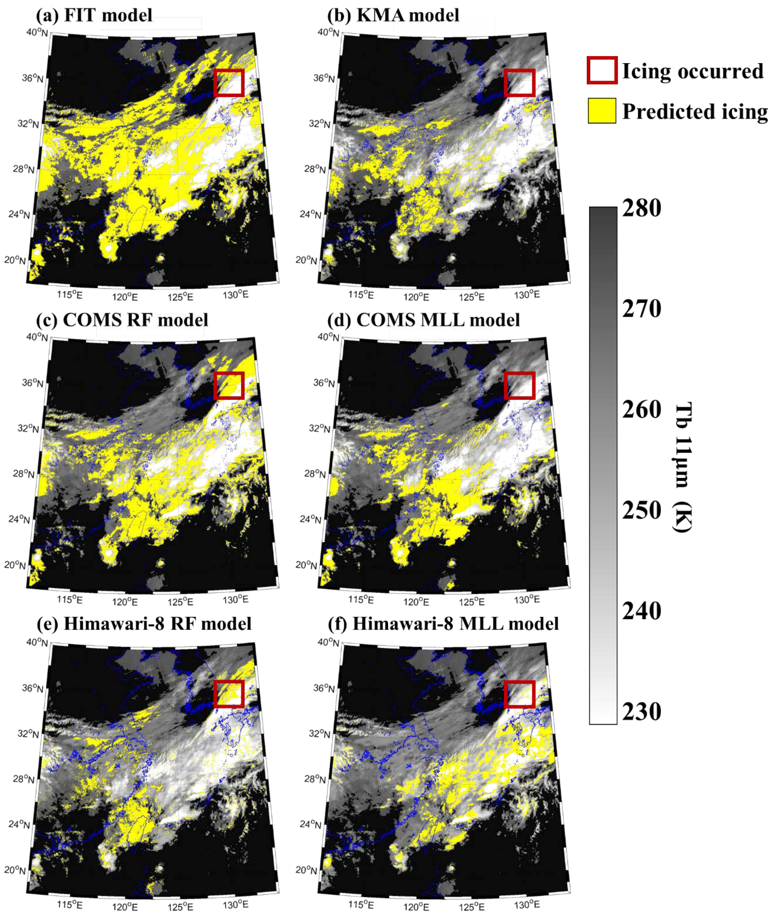
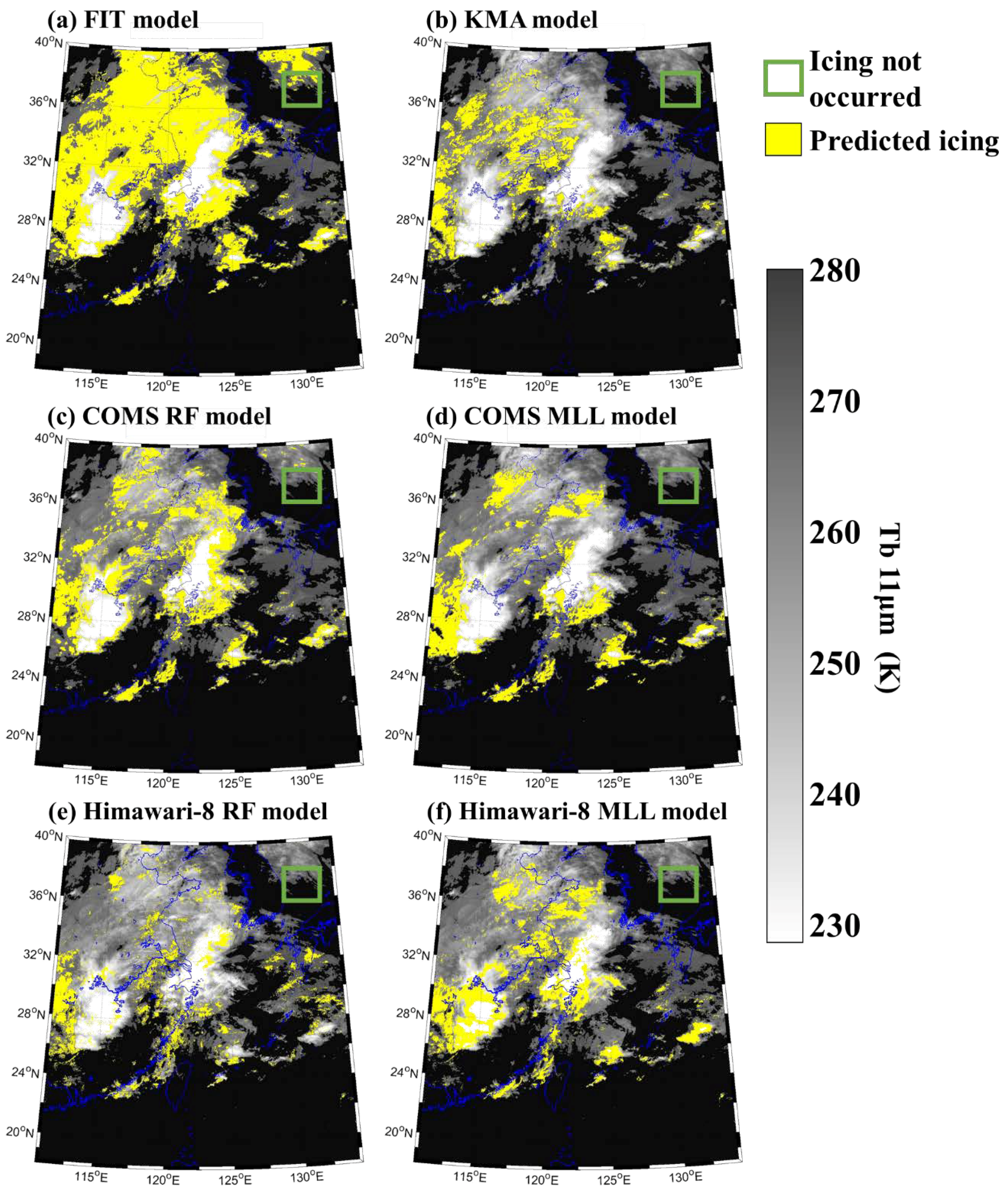
Figure 5 and Figure 6 depict the distribution of the potential icing areas produced from the six models as examples for selected icing and non-icing PIREP cases. Among the six models, the FIT model identified more low cloud areas as potential icing regions compared to the other models. This pattern often occurred when the phase of low clouds was SLW for other cases (not shown). However, such a pattern was not found where the cloud phase was neither water nor mixed.
Among the empirical machine learning models, the Himawari-8-based models classified less areas as potential icing clouds than the COMS based models when the same algorithm was used. This is possibly because a smaller number of training samples were available for the Himawari-8 models (Table 3), which often results in overfitting [62,63]. In particular, the ranges of the input values of the icing samples for the Himawari-8-based models were generally smaller than those for COMS-based models. The RF models produced a more scattered icing pattern in a number of small patches, while the MLL models showed more clustered icing regions. These patterns were consistently found in other cases (not shown). Although all machine-learning-based models produced high PODs, the MLL models did not correctly identify the icing/non-icing cases shown in Figure 5 and Figure 6. In summary, the COMS RF model and the Himawari-8 RF model resulted in the best performance in both the quantitative and qualitative analyses.
4.3. Temporal Variation of Icing
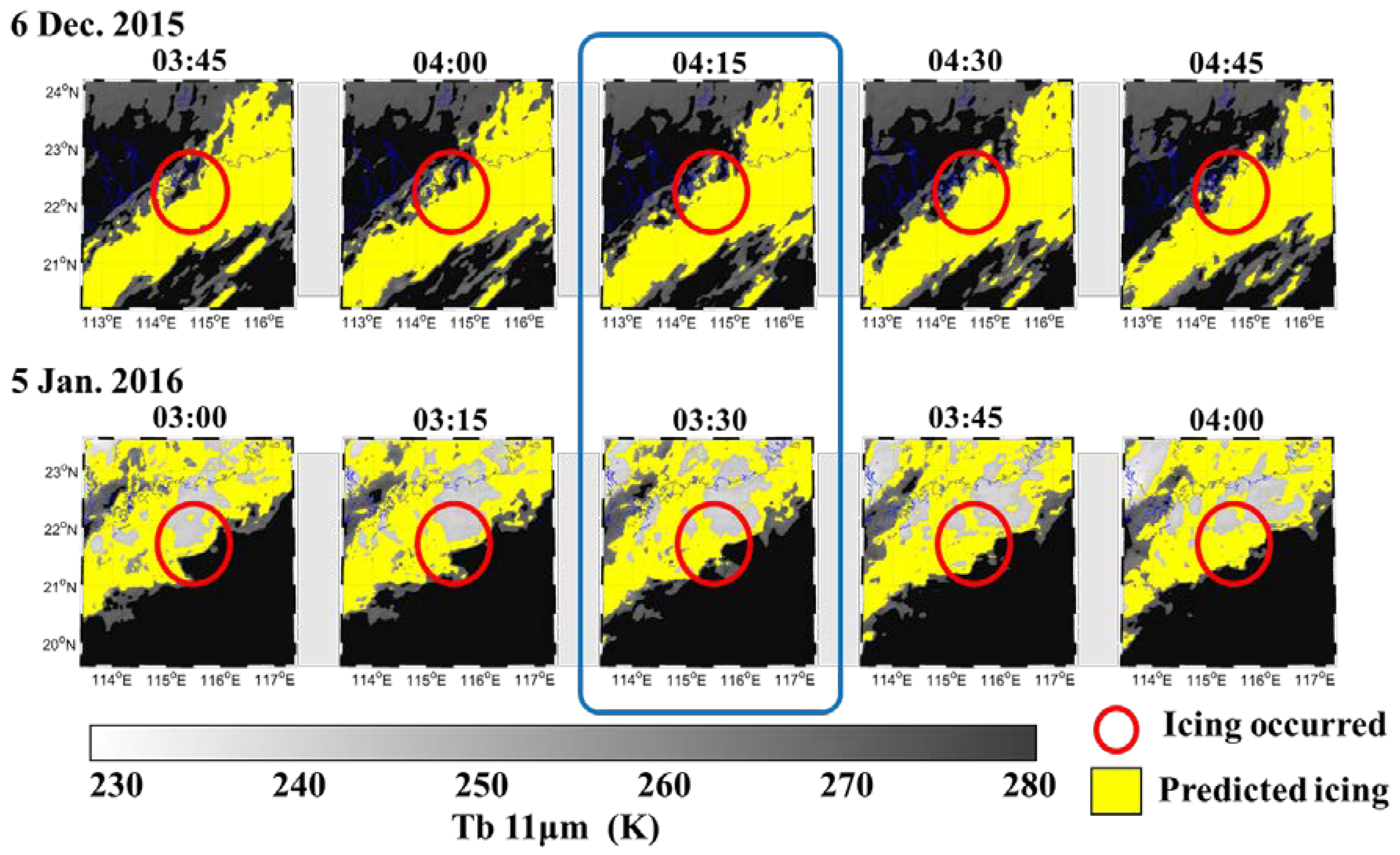
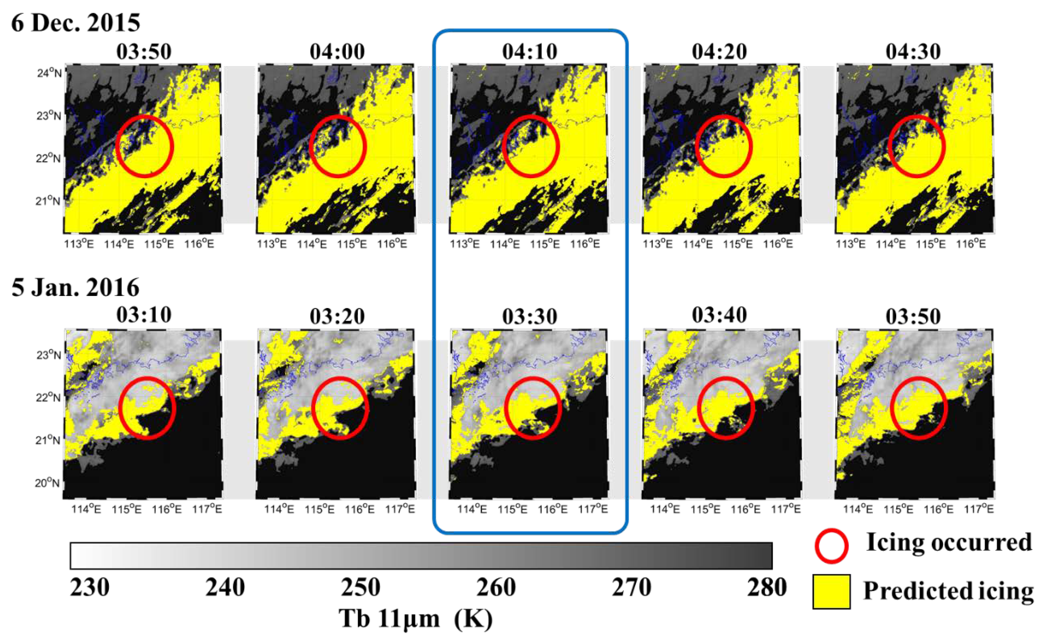
The spatial–temporal distribution of potential icing clouds was examined using COMS and Himawari-8 time-series data for two selected icing cases. The COMS RF and Himawari-8 RF models yielding the best performance were used to monitor potential icing areas (Figure 7 and Figure 8). A 15 min interval was used for the COMS RF model, while a 10 min interval was applied for the Himawari-8 RF model. Although the Himawari-8 RF model detected more areas with relatively warm clouds (Tb ~ 270 K) as potential icing regions and depicted a relatively sharper pattern, there was no abrupt change in the spatial distribution of the time-series icing maps. Similarly, the COMS RF results for the 5 January 2016 03:30 UTC series showed no drastic changes over time. This implies that both models are relatively stable considering the typical temporal variation of atmospheric conditions. In addition, potential icing areas often occur and decay rapidly in small patches, which indicates that icing detection can greatly benefit from satellite observations from geostationary sensor systems with a high temporal resolution (~10 min).
4.4. Novelty and Limitations
This study has proposed several machine-learning-based approaches for the detection of potential icing clouds, and compared their performance to the existing physical-theory-based models. The proposed models produced better performance than the existing models, which are based on simple rule-based approaches for the reference data available in this study. The superiority of the proposed models is partly due to the uncertainty of the satellite-derived products used in the existing physical-theory-based models. For example, the fraction correct for COMS CPH was reported as 0.642 when compared to Moderate Resolution Imaging Spectroradiometer (MODIS) data [66]. Similarly, the COMS COT yielded a root mean square error (RMSE) of 3.45 when compared to the MODIS COT [67]. Using such products as inputs for the threshold-based rules may result in a significant increase in uncertainty. The simple threshold-based rules used in the existing models might not be sufficient to model the complex characteristics of potential icing areas. By using additional input variables other than those used in the existing models, the proposed approaches were able to provide more accurate results with more sophisticated modeling techniques. The stable distribution of potential icing time-series confirmed the robustness of the proposed approaches.
However, there are several limitations to this study. First of all, the proposed models are heavily dependent on the reference data (i.e., PIREPs). Although careful quality control was conducted to secure accurate icing and non-icing samples, there is no guarantee that the selected icing and non-icing samples cover all possible icing and non-icing clouds. In particular, it is possible that potential icing areas may be missed simply because there is no visually identifiable icing phenomenon, which often leads to the underestimation of icing regions [68]. Not only the quality of the PIREPs, but also the number of PIREPs, is important to develop successful machine-learning-based icing detection models. For example, there are many PIREPs (more than 20,000) over CONUS for winter from 2006–2008 [15], which is ideal for the development of machine-learning-based models. However, only a small number of icing PIREPs are available in East Asia, which is a major limitation of this research. Such a small sample size often results in overfitting [62,63]. Since satellite-derived products typically provide information on the characteristics of cloud tops, it should be noted that PIREP-based icing information collected far below the cloud tops is not always closely related to satellite-derived cloud top products.
5. Conclusions
In this study, several machine-learning-based icing detection models were proposed and compared to the existing physical-theory-based models using COMS and Himawari-8 satellite data. Two machine learning approaches—RF and MLL—were used to develop the icing detection models. Both machine learning-based models resulted in better performance (POD of 68–82% and POFD of 16–18%) than those of the existing physical-theory-based models (POD of 12–36% and POFD of 7–27%) when COMS data were used. Overall, the RF models produced better performance than the MLL models according to the five-fold cross validation. However, the RF models resulted in higher standard errors in the performance metrics than the MLL models, which implies a tendency for overfitting. The variable importance identified by the machine learning models generally followed the physical characteristics of icing, e.g., resulting in high contributions by cloud top height.
Icing occurs in a variety of meteorological conditions, and thus a number of reference data collected from such conditions are required to develop more robust icing detection models. Although a small amount of qualified PIREP data, which might only cover a subset of those conditions, were used to develop the machine-learning-based icing detection models in this study, the results are promising. Therefore, the models deserve further research with more qualified reference data in order for governmental agencies to adopt such an approach from an operational perspective. The proposed approaches will be refined when more quality-controlled PIREP data become available. They will also be evaluated and optimized for the Geo-Kompsat-2 Advanced Meteorological Imager, which will be launched later in 2018 by the Korean government. In addition, the synergistic use of empirical machine learning and physical-theory-based models will be investigated to improve the detection of potential icing areas in the future.
Acknowledgments
This work was supported by the Development of Geostationary Meteorological Satellite Ground Segment (NMSC-2014-01) program, funded by the National Meteorological Satellite Centre (NMSC) of the Korea Meteorological Administration (KMA).
Author Contributions
Seongmun Sim led manuscript writing and contributed to the data analysis and research design. Jungho Im supervised this study, contributed to the research design and manuscript writing, and served as the corresponding author. Sumin Park and Haemi Park contributed to data processing and analysis. Myoung Hwan Ahn and Pak-wai Chan contributed to the discussion of the results and manuscript writing.
Conflicts of Interest
The authors declare no conflict of interest.
References
- Shappell, S.; Hackworth, C.; Holcomb, K.; Lanicci, J.; Bazargan, M.; Baron, J.; Iden, R.; Halperin, D. Developing Proactive Methods for General Aviation Data Collection; Clemson University, South Carolina: Clemson, SC, USA, 2010. [Google Scholar]
- Petty, K.R.; Floyd, C.D. In A statistical review of aviation airframe icing accidents in the US. In Proceedings of the 11th Conference on Aviation, Range, and Aerospace Hyannis, Hyannis, MA, USA, 3–8 October 2004. [Google Scholar]
- Alexandrov, M.D.; Cairns, B.; Van Diedenhoven, B.; Ackerman, A.S.; Wasilewski, A.P.; McGill, M.J.; Yorks, J.E.; Hlavka, D.L.; Platnick, S.E.; Arnold, G.T. Polarized view of supercooled liquid water clouds. Remote Sens. Environ. 2016, 181, 96–110. [Google Scholar] [CrossRef]
- Jung, S.; Tiwari, M.K.; Doan, N.V.; Poulikakos, D. Mechanism of supercooled droplet freezing on surfaces. Nat. Commun. 2012, 3, 615. [Google Scholar] [CrossRef] [PubMed]
- Politovich, M.K. Aircraft icing caused by large supercooled droplets. J. Appl. Meteorol. 1989, 28, 856–868. [Google Scholar] [CrossRef]
- Thompson, G.; Bullock, R.; Lee, T.F. Using satellite data to reduce spatial extent of diagnosed icing. Weather Forecast. 1997, 12, 185–190. [Google Scholar] [CrossRef]
- Schwartz, B. The quantitative use of pireps in developing aviation weather guidance products. Weather Forecast. 1996, 11, 372–384. [Google Scholar] [CrossRef]
- Ellrod, G.P. The Use of Goes-8 Multispectral Imagery for the Detection of Aircraft Icing Regions; NASA: Washington, DC, USA, 1996.
- Brown, B.G.; Thompson, G.; Bruintjes, R.T.; Bullock, R.; Kane, T. Intercomparison of in-flight icing algorithms. Part II: Statistical verification results. Weather Forecast. 1997, 12, 890–914. [Google Scholar] [CrossRef]
- Bernstein, B.C.; McDonough, F.; Politovich, M.K.; Brown, B.G.; Ratvasky, T.P.; Miller, D.R.; Wolff, C.A.; Cunning, G. Current icing potential: Algorithm description and comparison with aircraft observations. J. Appl. Meteorol. 2005, 44, 969–986. [Google Scholar] [CrossRef]
- Benjamin, S.G.; Dévényi, D.; Weygandt, S.S.; Brundage, K.J.; Brown, J.M.; Grell, G.A.; Kim, D.; Schwartz, B.E.; Smirnova, T.G.; Smith, T.L. An hourly assimilation—Forecast cycle: The ruc. Mon. Weather Rev. 2004, 132, 495–518. [Google Scholar] [CrossRef]
- Wang, P.; Li, J.; Li, J.; Li, Z.; Schmit, T.J.; Bai, W. Advanced infrared sounder subpixel cloud detection with imagers and its impact on radiance assimilation in NWP. Geophys. Res. Lett. 2014, 41, 1773–1780. [Google Scholar] [CrossRef]
- Kind, R.; Potapczuk, M.; Feo, A.; Golia, C.; Shah, A. Experimental and computational simulation of in-flight icing phenomena. Prog. Aerosp. Sci. 1998, 34, 257–345. [Google Scholar] [CrossRef]
- Rauber, R.M.; Tokay, A. An explanation for the existence of supercooled water at the top of cold clouds. J. Atmos. Sci. 1991, 48, 1005–1023. [Google Scholar] [CrossRef]
- Smith, W.L., Jr.; Minnis, P.; Fleeger, C.; Spangenberg, D.; Palikonda, R.; Nguyen, L. Determining the flight icing threat to aircraft with single-layer cloud parameters derived from operational satellite data. J. Appl. Meteorol. Climatol. 2012, 51, 1794–1810. [Google Scholar] [CrossRef]
- Minnis, P.; Nguyen, L.; Smith, W., Jr.; Young, D.; Khaiyer, M.; Palikonda, R.; Spangenberg, D.; Doelling, D.; Phan, D.; Nowicki, G. Real-Time Cloud, Radiation, and Aircraft Icing Parameters from Goes over the USA; NASA: Washington, DC, USA, 2004.
- Thompson, G.; Bruintjes, R.T.; Brown, B.G.; Hage, F. Intercomparison of in-flight icing algorithms. Part I: Wisp94 real-time icing prediction and evaluation program. Weather Forecast. 1997, 12, 878–889. [Google Scholar] [CrossRef]
- Isaac, G.; Cober, S.; Strapp, J.; Hudak, D.; Ratvasky, T.; Marcotte, D.; Fabry, F. In Preliminary results from the alliance icing research study (airs). In Proceedings of the 39th Aerospace Sciences Meeting and Exhibit, East Hartford, CT, USA, 8–11 January 2001; p. 393. [Google Scholar]
- Serke, D.J.; Politovich, M.K.; Reehorst, A.L.; Gaydos, A. Use of x-band radars to support the detection of in-flight icing hazards. J. Appl. Remote Sens. 2009, 3, 033532. [Google Scholar] [CrossRef]
- Bernstein, B.C.; Le Bot, C. An inferred climatology of icing conditions aloft, including supercooled large drops. Part II: Europe, Asia, and the globe. J. Appl. Meteorol. Climatol. 2009, 48, 1503–1526. [Google Scholar] [CrossRef]
- Minnis, P.; Smith, W., Jr.; Bedka, K.M.; Nguyen, L.; Palikonda, R.; Hong, G.; Trepte, Q.; Chee, T.; Scarino, B.; Spangenberg, D. Near-Real Time Satellite-Retrieved Cloud and Surface Properties for Weather and Aviation Safety Applications; AGU Fall Meeting Abstracts; American Geophysical Union: Washington, DC, USA, 2014. [Google Scholar]
- Choi, M.-B.; Kim, O.; Cha, E.; Yoo, S.-J. Development and verification of icing algorithm using communication, ocean and meteorological satellite (coms). In Proceedings of the Autumn Meeting of KMS, Jeju-island, Korea, 13–15 October 2014; pp. 715–716. [Google Scholar]
- Im, J.; Jensen, J.R.; Jensen, R.R.; Gladden, J.; Waugh, J.; Serrato, M. Vegetation cover analysis of hazardous waste sites in Utah and Arizona using hyperspectral remote sensing. Remote Sens. 2012, 4, 327–353. [Google Scholar] [CrossRef]
- Li, M.; Im, J.; Beier, C. Machine learning approaches for forest classification and change analysis using multi-temporal landsat tm images over huntington wildlife forest. GISci. Remote Sens. 2013, 50, 361–384. [Google Scholar]
- Kim, Y.H.; Im, J.; Ha, H.K.; Choi, J.-K.; Ha, S. Machine learning approaches to coastal water quality monitoring using goci satellite data. GISci. Remote Sens. 2014, 51, 158–174. [Google Scholar] [CrossRef]
- Rhee, J.; Im, J.; Carbone, G.; Jensen, J. Delineation of climate regions using in-situ and remotely-sensed data for the Carolinas. Remote Sens. Environ. 2008, 112, 3099–3111. [Google Scholar] [CrossRef]
- Lu, Z.; Im, J.; Quackenbush, L. A volumetric approach to population estimation using LiDAR remote sensing. Photogramm. Eng. Remote Sens. 2011, 77, 1145–1156. [Google Scholar]
- Park, M.-S.; Kim, M.; Lee, M.-I.; Im, J.; Park, S. Detection of tropical cyclone genesis via quantitative satellite ocean surface wind pattern and intensity analyses using decision trees. Remote Sens. Environ. 2016, 183, 205–214. [Google Scholar] [CrossRef]
- Han, H.; Lee, S.; Im, J.; Kim, M.; Lee, M.-I.; Ahn, M.H.; Chung, S.-R. Detection of convective initiation using meteorological imager onboard communication, ocean, and meteorological satellite based on machine learning approaches. Remote Sens. 2015, 7, 9184–9204. [Google Scholar] [CrossRef]
- Kim, M.; Im, J.; Park, H.; Park, S.; Lee, M.-I.; Ahn, M.-H. Detection of tropical overshooting cloud tops using himawari-8 imagery. Remote Sens. 2017, 9, 685. [Google Scholar] [CrossRef]
- Lee, S.; Han, H.; Im, J.; Jang, E.; Lee, M.-I. Detection of deterministic and probabilistic convection initiation using Himawari-8 advanced Himawari imager data. Atmos. Meas. Tech. 2017, 10, 1859–1874. [Google Scholar] [CrossRef]
- Airports Council International. ACI Releases Preliminary 2016 World Airport Traffic Rankings—Robust Gains in Passenger Traffic at Hub Airports Serving Trans-PACIFIC and East Asian Routes. Available online: http://www.aci.aero/News/Releases/Most-Recent/2017/04/19/ACI-releases-preliminary-2016-world-airport-traffic-rankingsRobust-gains-in-passenger-traffic-at-hub-airports-serving-transPacific-and-East-Asian-routes (accessed on 19 April 2017).
- Choi, Y.S.; Ho, C.H.; Ahn, M.H.; Kim, Y.M. An exploratory study of cloud remote sensing capabilities of the communication, ocean and meteorological satellite (coms) imagery. Int. J. Remote Sens. 2007, 28, 4715–4732. [Google Scholar]
- King, M.D.; Tsay, S.-C.; Platnick, S.E.; Wang, M.; Liou, K.-N. Cloud Retrieval Algorithms for Modis: Optical Thickness, Effective Particle Radius, and Thermodynamic Phase; MODIS Algorithm Theoretical Basis Document, 1997. Available online: http://patarnott.com/satsens/pdf/CloudRetrieval_atbd_mod05.pdf (accessed on 17 April 2018).
- Menzel, P.; Strabala, K. Cloud Top Properties and Cloud Phase Algorithm Theoretical Basis Document; University of Wisconsin-Madison: Madison, WI, USA, 1997. [Google Scholar]
- Da, C. Preliminary assessment of the Advanced Himawari Imager (AHI) measurement onboard Himawari-8 geostationary satellite. Remote Sens. Lett. 2015, 6, 637–646. [Google Scholar] [CrossRef]
- Kurihara, Y.; Murakami, H.; Kachi, M. Sea surface temperature from the new Japanese geostationary meteorological Himawari-8 satellite. Geophys. Res. Lett. 2016, 43, 1234–1240. [Google Scholar] [CrossRef]
- Yumimoto, K.; Nagao, T.; Kikuchi, M.; Sekiyama, T.; Murakami, H.; Tanaka, T.; Ogi, A.; Irie, H.; Khatri, P.; Okumura, H. Aerosol data assimilation using data from Himawari-8, a next-generation geostationary meteorological satellite. Geophys. Res. Lett. 2016, 43, 5886–5894. [Google Scholar] [CrossRef]
- Thompson, G.; Politovich, M.K.; Rasmussen, R.M. A numerical weather model’s ability to predict characteristics of aircraft icing environments. Weather Forecast. 2017, 32, 207–221. [Google Scholar] [CrossRef]
- Choi, Y.-S.; Lindzen, R.S.; Ho, C.-H.; Kim, J. Space observations of cold-cloud phase change. Proc. Natl. Acad. Sci. USA 2010, 107, 11211–11216. [Google Scholar] [CrossRef] [PubMed]
- Kühnlein, M.; Appelhans, T.; Thies, B.; Nauss, T. Improving the accuracy of rainfall rates from optical satellite sensors with machine learning—A random forests-based approach applied to MSG SEVIRI. Remote Sens. Environ. 2014, 141, 129–143. [Google Scholar] [CrossRef]
- Tu, J.V. Advantages and disadvantages of using artificial neural networks versus logistic regression for predicting medical outcomes. J. Clin. Epidemiol. 1996, 49, 1225–1231. [Google Scholar] [CrossRef]
- Autonès, F. Algorithm Theoretical Basis Document for “Rapid Development Thunderstorms” (RDT-PGE11 v3.0); METEO-FRANCE: Paris, France, 2013. [Google Scholar]
- Breiman, L. Random forests. Mach. Learn. 2001, 45, 5–32. [Google Scholar] [CrossRef]
- Richardson, H.; Hill, D.; Denesiuk, D.; Fraser, L. A comparison of geographic datasets and field measurements to model soil carbon using random forests and stepwise regressions (British Columbia, Canada). GISci. Remote Sens. 2017, 54, 573–591. [Google Scholar] [CrossRef]
- Amani, M.; Salehi, B.; Mahdavi, S.; Granger, J.; Brisco, B. Wetland classification in Newfoundland and Labrador using multi-source SAR and optical data integration. GISci. Remote Sens. 2017, 54, 779–796. [Google Scholar] [CrossRef]
- Lu, Z.; Im, J.; Rhee, J.; Hodgson, M. Building type classification using spatial and landscape attributes derived from LiDAR remote sensing data. Landsc. Urban Plan. 2014, 130, 134–148. [Google Scholar] [CrossRef]
- Guo, Z.; Du, S. Mining parameter information for building extraction and change detection with very high resolution imagery and GIS data. GISci. Remote Sens. 2017, 54, 38–63. [Google Scholar] [CrossRef]
- Li, M.; Im, J.; Quackenbush, L.; Liu, T. Forest biomass and carbon stock quantification using airborne LiDAR data: A case study over Huntington Wildlife Forest in the Adirondack Park. IEEE J. Sel. Top. Appl. Earth Obs. Remote Sens. 2014, 7, 3143–3156. [Google Scholar] [CrossRef]
- Forkuor, G.; Dimobe, K.; Serme, I.; Tondoh, J. Landsat-8 vs. Sentinel-2: Examining the added value of sentinel-2′s red-edge bands to land-use and land-cover mapping in Burkina Faso. GISci. Remote Sens. 2018, 55, 331–354. [Google Scholar] [CrossRef]
- Jang, E.; Im, J.; Park, G.; Park, Y. Estimation of fugacity of carbon dioxide in the East Sea using in situ measurements and Geostationary Ocean Color Imager satellite data. Remote Sens. 2017, 9, 821. [Google Scholar] [CrossRef]
- Millard, K.; Richardson, M. On the importance of training data sample selection in random forest image classification: A case study in peatland ecosystem mapping. Remote Sens. 2015, 7, 8489–8515. [Google Scholar]
- Park, S.; Im, J.; Jang, E.; Rhee, J. Drought assessment and monitoring through blending of multi-sensor indices using machine learning approaches for different climate regions. Agric. For. Meteorol. 2016, 216, 157–169. [Google Scholar]
- Yoo, C.; Im, J.; Park, S.; Quackenbush, L. Estimation of daily maximum and minimum air temperature in urban landscapes using MODIS time series satellite data. ISPRS J. Photogramm. Remote Sens. 2018, 137, 149–162. [Google Scholar] [CrossRef]
- Benoit, K. Linear Regression Models with Logarithmic Transformations; London School of Economics: London, UK, 2011; Available online: http://kenbenoit.net/assets/courses/ME104/logmodels2.pdf (accessed on 17 April 2018).
- Venables, W.N.; Ripley, B.D. Modern Applied Statistics with s-Plus; Springer Science & Business Media: Berlin, Germany, 2013. [Google Scholar]
- Ripley, B.; Venables, W.; Ripley, M.B. Package ‘nnet’; R Package Version 2016, 7.3-12. Available online: https://cran.r-project.org/web/packages/nnet/nnet.pdf (accessed on 17 April 2018).
- Smith, W.L., Jr.; Minnis, P.; Fleeger, C. Algorithm Theoretical Basis Document: Flight Icing Threat; NOAA NESDIS Center for Satellite Applications and Research: Silver Spring, MD, USA, 2010.
- AghaKouchak, A.; Mehran, A. Extended contingency table: Performance metrics for satellite observations and climate model simulations. Water Resour. Res. 2013, 49, 7144–7149. [Google Scholar] [CrossRef]
- Han, H.; Im, J.; Kim, M.; Sim, S.; Kim, J.; Kim, D.-J.; Kang, S.-H. Retrieval of melt ponds on arctic multiyear sea ice in summer from terrasar-x dual-polarization data using machine learning approaches: A case study in the chukchi sea with mid-incidence angle data. Remote Sens. 2016, 8, 57. [Google Scholar] [CrossRef]
- Kim, M.; Im, J.; Han, H.; Kim, J.; Lee, S.; Shin, M.; Kim, H.-C. Landfast sea ice monitoring using multisensor fusion in the antarctic. GISci. Remote Sens. 2015, 52, 239–256. [Google Scholar] [CrossRef]
- Louppe, G.; Wehenkel, L.; Sutera, A.; Geurts, P. Understanding variable importances in forests of randomized trees. In Advances in Neural Information Processing Systems; Burges, C.J.C., Bottou, L., Welling, M., Ghahramani, Z., Weinberger, K.Q., Eds.; NIPS Foundation: La Jolla, CA, USA, 2013; pp. 431–439. [Google Scholar]
- Rhee, J.; Im, J. Meteorological drought forecasting for ungauged areas based on machine learning: Using long-range climate forecast and remote sensing data. Agric. For. Meteorol. 2017, 237, 105–122. [Google Scholar] [CrossRef]
- Wolters, E.L.; Roebeling, R.A.; Feijt, A.J. Evaluation of cloud-phase retrieval methods for seviri on meteosat-8 using ground-based lidar and cloud radar data. J. Appl. Meteorol. Climatol. 2008, 47, 1723–1738. [Google Scholar] [CrossRef]
- Schmit, T.J.; Gunshor, M.M.; Menzel, W.P.; Gurka, J.J.; Li, J.; Bachmeier, A.S. Introducing the next-generation advanced baseline imager on GOES-R. Bull. Am. Meteorol. Soc. 2005, 86, 1079–1096. [Google Scholar] [CrossRef]
- Choi, Y.S.; Cho, H. Algorithm Theoretical Basis Document for Cloud Phase; National Meteorological Satellite Center: Chungcheongbuk-do, Korea, 2012.
- Choi, Y.S.; Cho, H. Algorithm Theoretical Basis Document for Cloud Optical Thickness; National Meteorological Satellite Center: Chungcheongbuk-do, Korea, 2012.
- Carrière, J.-M.; Lainard, C.; Le Bot, C.; Robart, F. A climatological study of surface freezing precipitation in Europe. Meteorol. Appl. 2000, 7, 229–238. [Google Scholar] [CrossRef]
Figure 1.
A flow chart of the proposed machine-learning-based icing detection approach.

Figure 2.
An example of icing and non-icing sample extraction from COMS data. Preprocessed images are masked using the threshold at the infrared-1 (IR1) channel and a spatial buffer. In this example, icing was reported on 5 July 2011 23:50 UTC at N37.42° and E129.2° and non-icing was reported on 5 July 2011 23:48 UTC at N36.58° and E130.25°.

Figure 3.
Relative variable importance identified by machine learning models. Mean decrease accuracy is calculated using out-of-bag samples when a variable is perturbed by random forest (RF). Absolute normalized coefficients are considered as a variable importance in the multinomial log-linear (MLL) models. The larger the value of a variable, the more significant the variable. The most significant (top 20%) variables are displayed in orange.

Figure 4.
Accuracy assessment results of each icing detection model. (POD = Probability of detection; POFD = Probability of false detection; OA = Overall accuracy; TSS = True skill statistics; E = Standard error).
Figure 4.
Accuracy assessment results of each icing detection model. (POD = Probability of detection; POFD = Probability of false detection; OA = Overall accuracy; TSS = True skill statistics; E = Standard error).

Figure 5.
Maps of potential icing areas produced by the six algorithms for the COMS and Himawari-8 images collected on 24 April 2016 01:00 UTC. The 11 μm channel Tb image ranging from 228 K to 280 K is used as the background image. Areas with no cloud or a Tb of 11 μm > 270 K were masked out and appear black in the figures.

Figure 6.
Maps of potential icing areas produced by the six algorithms for the COMS and Himawari-8 images collected on 26 April 2016 01:00 UTC. The 11 μm channel Tb image ranging from 228 K to 280 K is used as the background image. Areas with no cloud or a Tb of 11 μm > 270 K were masked out and appear black in the figures.

Figure 7.
Time-series of potential icing areas when the COMS RF model was applied for two icing cases (i.e., the upper images on 6 December 2015 04:15 UTC with an icing pilot report (PIREP) at E22.19° and N114.60° and the bottom images on 5 January 2016 03:30 UTC with an icing PIREP at E21.58° and N115.41°). The corresponding 11 μm channel images were used as the background.

Figure 8.
Time-series of potential icing areas when the Himawari-8 RF model was applied for two icing cases (i.e., the upper images on 6 December 2015 04:15 UTC at E22.19° and N114.60° and the bottom images on 5 January 2016 03:30 UTC at E21.58° and N115.41°). The corresponding 11 μm channel images were used as the background.


Table 1.
Specification of variables of Communication, Ocean and Meteorological Satellite (COMS) Meteorological Imager (MI) and Himawari-8 Advanced Himawari Imager (AHI) used in developing icing detection models in this study (Tb = Brightness temperature).
Table 1.
Specification of variables of Communication, Ocean and Meteorological Satellite (COMS) Meteorological Imager (MI) and Himawari-8 Advanced Himawari Imager (AHI) used in developing icing detection models in this study (Tb = Brightness temperature).
| COMS MI | Himawari-8 AHI | |||||
|---|---|---|---|---|---|---|
| Variable Name | Description | Resolution | Variable Name | Description | Resolution | |
| Level 1b | CH01 | Albedo of 0.43–0.48 µm channel | 1 km | |||
| Visible | Albedo of 0.55–0.80 µm channel | 1 km | CH02 | Albedo of 0.50–0.52 µm channel | ||
| SWIR | Tb of 3.5–4.0 µm channel | 4 km | CH04 | Albedo of 0.85–0.87 µm channel | ||
| WV | Tb of 6.5–7.0 µm channel | CH05 | Albedo of 1.60–1.62 µm channel | 2 km | ||
| IR1 | Tb of 10.3–11.3 µm channel | CH06 | Albedo of 2.25–2.27 µm channel | |||
| IR2 | Tb of 11.5–12.5 µm channel | CH07 | Tb of 3.74–3.96 µm channel | |||
| BTD1 | Tb difference between SWIR and IR1 | CH08 | Tb of 6.06–6.43 µm channel | |||
| BTD2 | Tb difference between IR1 and IR2 | CH09 | Tb of 6.89–7.01 µm channel | |||
| Level 2 | CH10 | Tb of 7.26–7.43 µm channel | ||||
| CLA | COT | Cloud optical thickness | 4 km | CH11 | Tb of 8.44–8.76 µm channel | |
| CP | Cloud phase | CH13 | Tb of 10.3–10.6 µm channel | |||
| CTTP | CTT | Cloud top temperature | CH14 | Tb of 11.1–11.3 µm channel | ||
| CTH | Cloud top height | CH15 | Tb of 12.2–12.5 µm channel | |||
| CTP | Cloud top pressure | CH16 | Tb of 13.2–13.4 µm channel | |||
Table 2.
Quality control rules for selecting pilot reports (PIREPs) to be used to develop icing detection models. Six rules were applied to each pixel in the buffer with a radius of 20 km at an icing PIREP location. Pixels that met the rules, except for rule 3, were excluded. A final decision as to whether an icing PIREP was valid or not was made using the remaining pixels within the buffer.
| Rule | Description | Satellite Sensor | Flag | |
|---|---|---|---|---|
| COMS | Himawari-8 | |||
| Rule 1 | Flight over a cloud top | FA * > CTH | FA > CTH | Excluded |
| Rule 2 | Flight near an ice cloud top | FA ~ CTH CPH = ICE | ̶ | Excluded |
| Rule 3 | Flight below a thick ice cloud top | FA < CTH CPH = ICE COT > 6 | FA < CTH R > 0.1 | Pass |
| Rule 4 | Flight below a thin ice cloud top | FA < CTH CPH = ICECOT ~ 0 | FA < CTH R < 0.1 | Excluded |
| Rule 5 | Flight near or below a warm cloud | Tb 11 μm > 270 K | Tb 11 μm > 270 K | Excluded |
| Rule 6 | Flight near or below a frigid cloud | Tb 11 μm < 228 K | Tb 11 μm < 228 K | Excluded |
| Final Decision | The remaining pixels that meet the rules > 20% of the buffer with a radius of 20 km | Valid | ||
* FA = Flight Altitude (m); CTH = Cloud Top Height (m); CPH = Cloud Phase; COT = Cloud Optical Thickness; Tb = Brightness temperature (K); R = Reflectance.
Table 3.
PIREP data used to develop icing detection models for COMS and Himawari-8. Values in parentheses are the number of icing PIREPs before conducting quality control, while the values in front of the parentheses are the number of icing PIREPs after the quality control.
Table 3.
PIREP data used to develop icing detection models for COMS and Himawari-8. Values in parentheses are the number of icing PIREPs before conducting quality control, while the values in front of the parentheses are the number of icing PIREPs after the quality control.
| COMS (April 2011–July 2017) | Himawari-8 (July 2015–July 2017) | |||
|---|---|---|---|---|
| Icing | Non-Icing | Icing | Non-Icing | |
| KMA | 12 (18) | 219 | 6 (8) | 59 |
| HKO | 21 (36) | 0 | 10 (16) | 0 |
| Sum | 33 (54) | 219 | 16 (24) | 59 |
Table 4.
Existing rule-based icing detection approaches (i.e., flight icing threat (FIT) and Korea meteorological administration (KMA) algorithms to produce icing mask).
Table 4.
Existing rule-based icing detection approaches (i.e., flight icing threat (FIT) and Korea meteorological administration (KMA) algorithms to produce icing mask).
| FIT Algorithm | KMA Algorithm | ||||||
|---|---|---|---|---|---|---|---|
| Cloud Phase | COT | Icing Mask | IR1 | Visible | SWIR–IR1 | IR1–IR2 | Icing Mask |
| Clear | ─ | No icing | 243 K ≤ Tb ≤ 272 K | Albedo ≥ 37% | BTD ≥ 10 K | BTD < 1 K | Icing |
| Water | All | No icing | 243 K ≤ Tb ≤ 272 K | Albedo ≥ 37% | BTD ≥ 10 K | BTD ≥ 1 K | No icing |
| SLW | τ > 1.0 | Icing | 243 K ≤ Tb ≤ 272 K | Albedo ≥ 37% | BTD < 10 K | ─ | No icing |
| SLW | τ ≤ 1.0 | No icing | 243 K ≤ Tb ≤ 272 K | 4.5% ≤ Albedo < 37% | ─ | ─ | No icing |
| Mixed | τ >1.0 | Icing | 243 K ≤ Tb ≤ 272 K | Albedo < 4.5% | BTD ≤ −2.5 K | BTD < 1 K | Icing |
| Mixed | τ ≤ 1.0 | No icing | 243 K ≤ Tb ≤ 272 K | Albedo < 4.5% | BTD ≤ −2.5 K | BTD ≥ 1 K | No icing |
| Ice | τ ≤ 6.0 | No icing | 243 K ≤ Tb ≤ 272 K | Albedo < 4.5% | BTD > −2.5 K | ─ | No icing |
| Ice | τ > 6.0 | Unknown | Tb < 243 K or Tb > 272 K | ─ | ─ | ─ | No icing |
Table 5.
A contingency table used in this study to calculate performance metrics.
| Reference | ||
|---|---|---|
| Model Classified | Non-Icing | Icing |
| Non-icing | Correct negative (N) | Miss (M) |
| Icing | False (F) | Hit (H) |
© 2018 by the authors. Licensee MDPI, Basel, Switzerland. This article is an open access article distributed under the terms and conditions of the Creative Commons Attribution (CC BY) license (http://creativecommons.org/licenses/by/4.0/).
Share and Cite
MDPI and ACS Style
Sim, S.; Im, J.; Park, S.; Park, H.; Ahn, M.H.; Chan, P.-w. Icing Detection over East Asia from Geostationary Satellite Data Using Machine Learning Approaches. Remote Sens. 2018, 10, 631. https://doi.org/10.3390/rs10040631
AMA Style
Sim S, Im J, Park S, Park H, Ahn MH, Chan P-w. Icing Detection over East Asia from Geostationary Satellite Data Using Machine Learning Approaches. Remote Sensing. 2018; 10(4):631. https://doi.org/10.3390/rs10040631
Chicago/Turabian StyleSim, Seongmun, Jungho Im, Sumin Park, Haemi Park, Myoung Hwan Ahn, and Pak-wai Chan. 2018. "Icing Detection over East Asia from Geostationary Satellite Data Using Machine Learning Approaches" Remote Sensing 10, no. 4: 631. https://doi.org/10.3390/rs10040631
Note that from the first issue of 2016, this journal uses article numbers instead of page numbers. See further details here.