Model Selection for Parametric Surfaces Approximating 3D Point Clouds for Deformation Analysis


Geodetic Institute, Leibniz Universität Hannover, Nienburger Str. 1, 30167 Hannover, Germany
*
Author to whom correspondence should be addressed.
Remote Sens. 2018, 10(4), 634; https://doi.org/10.3390/rs10040634
Submission received: 20 February 2018
/
Revised: 11 April 2018
/
Accepted: 16 April 2018
/
Published: 19 April 2018
(This article belongs to the Special Issue 3D Modelling from Point Clouds: Algorithms and Methods)
Abstract
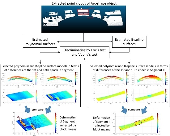
:Deformation monitoring of structures is a common application and one of the major tasks of engineering surveying. Terrestrial laser scanning (TLS) has become a popular method for detecting deformations due to high precision and spatial resolution in capturing a number of three-dimensional point clouds. Surface-based methodology plays a prominent role in rigorous deformation analysis. Consequently, it is of great importance to select an appropriate regression model that reflects the geometrical features of each state or epoch. This paper aims at providing the practitioner some guidance in this regard. Different from standard model selection procedures for surface models based on information criteria, we adopted the hypothesis tests from D.R. Cox and Q.H. Vuong to discriminate statistically between parametric models. The methodology was instantiated in two numerical examples by discriminating between widely used polynomial and B-spline surfaces as models of given TLS point clouds. According to the test decisions, the B-spline surface model showed a slight advantage when both surface types had few parameters in the first example, while it performed significantly better for larger numbers of parameters. Within B-spline surface models, the optimal one for the specific segment was fixed by Vuong’s test whose result was quite consistent with the judgment of widely used Bayesian information criterion. The numerical instabilities of B-spline models due to data gap were clearly reflected by the model selection tests, which rejected inadequate B-spline models in another numerical example.
1. Introduction
Deformation monitoring of engineering structures such as bridges, tunnels, dams, and tall buildings is a common application of engineering surveying [1]. As summarized in Mukupa et al. [2], deformation analysis can be based on different comparison objects, namely, point-to-point, point-to-surface, or surface-to-surface. The point-to-point-based analysis is a common approach to describe deformations that are captured by conventional point-wise surveying techniques. Examples of such techniques are the total station and the global navigation satellite system; however, in many cases, these have been surpassed by the use of LiDAR technology, especially terrestrial laser scanning (TLS) [3,4]. Although the single-point precision of TLS is in the sub-centimeter range ( to mm), the high redundancy of the scanning observations facilitates a higher precision via the application of least-squares based curve or surface estimation and, hence, an adequate precision of the estimated deformation parameters [5]. A point-to-surface-based analysis is carried out to represent a deformation by the distance between the point cloud in one epoch and the surface estimated from measurements in another epoch. Such a surface can be constructed as a polygonal model (mesh) [6,7,8] or as a regression model (e.g., a polynomial or B-spline surface model) [9,10,11,12,13]. The procedure of a surface-to-surface-based deformation analysis, which is appropriate in certain situations, is to divide the point clouds into cells and to compare the parameters of fitted planes based on cell points in two epochs. This method is applied in Lindenbergh et al. [14], where the different positions of the laser scanner and strong wind contribute to the change of the coordinate system. The aforementioned three approaches to deformation analysis are complemented by the “point-cloud-based” approach, in which a deformation is reflected by the parameters of a coordinate transformation between sets of point clouds in various epochs. The common algorithm for determining the transformation matrix is the iterative closest point algorithm. The authors of Girardeau-Montaut et al. [15] presented three simple cloud-to-cloud comparison techniques for detecting changes in building sites or indoor facilities within a certain time.
Aiming at rigorous deformation detection from scatter point clouds, it is crucial to describe the geometrical features of the object accurately by an appropriate curve or surface regression model, and emphasis is put on the latter model in this paper. The purpose of surface fitting is to estimate the continuous model function from the scatter point samples, which can be implemented by approximation in the case of redundant measurements. There are many approximation approaches for working with surfaces based on an implicit, explicit, or parametric form. Parametric models are usually employed to fit point cloud data in applications such as deformation monitoring and reverse engineering. Different parametric models perform differently in terms of accuracy and number of coefficients when fitted to a dataset. Among the many methods utilized in various applications for approximating point clouds, polynomial model fitting is usually applied to smooth and regular objects due to its simple operation. In [16], the authors assumed a concrete arch as regular and analyzed the deformation behavior through comparing fitted second-degree polynomial surfaces. The more involved fitting of B-splines and non-uniform rational basis splines is often preferred for modeling geometrically complicated objects. In this context, much research has focused on the optimization of the mathematical and stochastic models. In Bureick et al. [17], the authors optimized free-form curve approximation by means of an optimal selection of the knot vector. Furthermore, in Harmening and Neuner [18], the authors improved the parametrization process in B-spline surface fitting by using an object-oriented approach instead of focusing on a superior coordinates system, thereby enabling the generated parameters to reflect the features of the object realistically. Moreover, in Zhao et al. [19], the authors suggested a new stochastic model for TLS measurements and used the resulting covariance matrix within the least-squares estimation of a B-spline curve.
The need for model selection and statistical validation was emphasized in Wunderlich et al. [20], the authors of which described the deficiencies in current areal deformation analysis and presented possible strategies to improve this situation. Typically, the selection of surface model depends on the object features—for example, whether the surface is regular or irregular. However, in most cases, it is unclear whether the object is smooth enough to be described by a simple model (e.g., as a low-order, global polynomial surface) or not. This limitation serves as the motivation for discriminating between estimated surface models in order to select the most appropriate one. In the context of model selection, Harmening and Neuner [21,22] investigated statistical methods based on information criteria and statistical learning theory for selecting the optimal number of control points within B-spline surface estimation. Another possibility is to compare the (log-)likelihoods of competing models directly by means of the general testing principle by D.R. Cox [23]. In Williams [24], the authors improved the Cox’s test based on the use of Monte-Carlo simulation, which is straightforward to implement. This kind of test has already been used in Zhao et al. [19] to select the best fitting stochastic model for B-spline curve estimation. In Vuong [25], the authors use likelihood-ratio-based statistics to discriminate the competing models based on Kullback–Leibler information criterion. Such hypothesis tests offer the advantage that significant probabilistic differences between models can be detected, which is information that has not been provided by the methods mentioned previously.
The motivation of this paper lies in the selection of the most parsimonious, yet sufficiently accurate, parametric description of structure based on TLS measurements, whose model is applied to reflect the surface-based deformation of measured objects. Different from standard model selections procedures based on information criteria, we introduce two likelihood-ratio tests from D.R. Cox and Q.H. Vuong, which are instantiated in numerical examples to discriminate statistically between widely used polynomial and B-spline surfaces as models of given TLS point clouds. The selected surface model’s performance in reflecting deformation is compared with the result of the block-means approach. The paper is organized as follows. In Section 2, the methodology of surface approximation and model selection is reviewed and explained. This methodology is instantiated in two numerical examples by discriminating between widely used polynomial and B-spline surfaces. The evaluation of approximated surface models as well as their performance in deformation analysis are given as results in Section 3. The subsequent Section 4 provides a further discussion on the results and a comparison with results obtained by some well-known penalization information criterion approaches. Finally, conclusions are drawn in Section 5.
2. Methodology
2.1. Experiment Design
An experiment was conducted jointly with the Institute of Concrete Construction of the Leibniz Universität Hannover to probe the load-caused behavior and ultimate bearing capacity of a concrete arch structure with a length of about 2 m and thickness of m. Loads were placed on top of the arch’s surface for 13 epochs, within which the load was exerted with a uniform speed (2 kN/min) of about 20 min followed by a break of approximately 10 min for data capture [9]. The weight of load was increased continuously and reached 520 kN at the end of the 13th epoch.
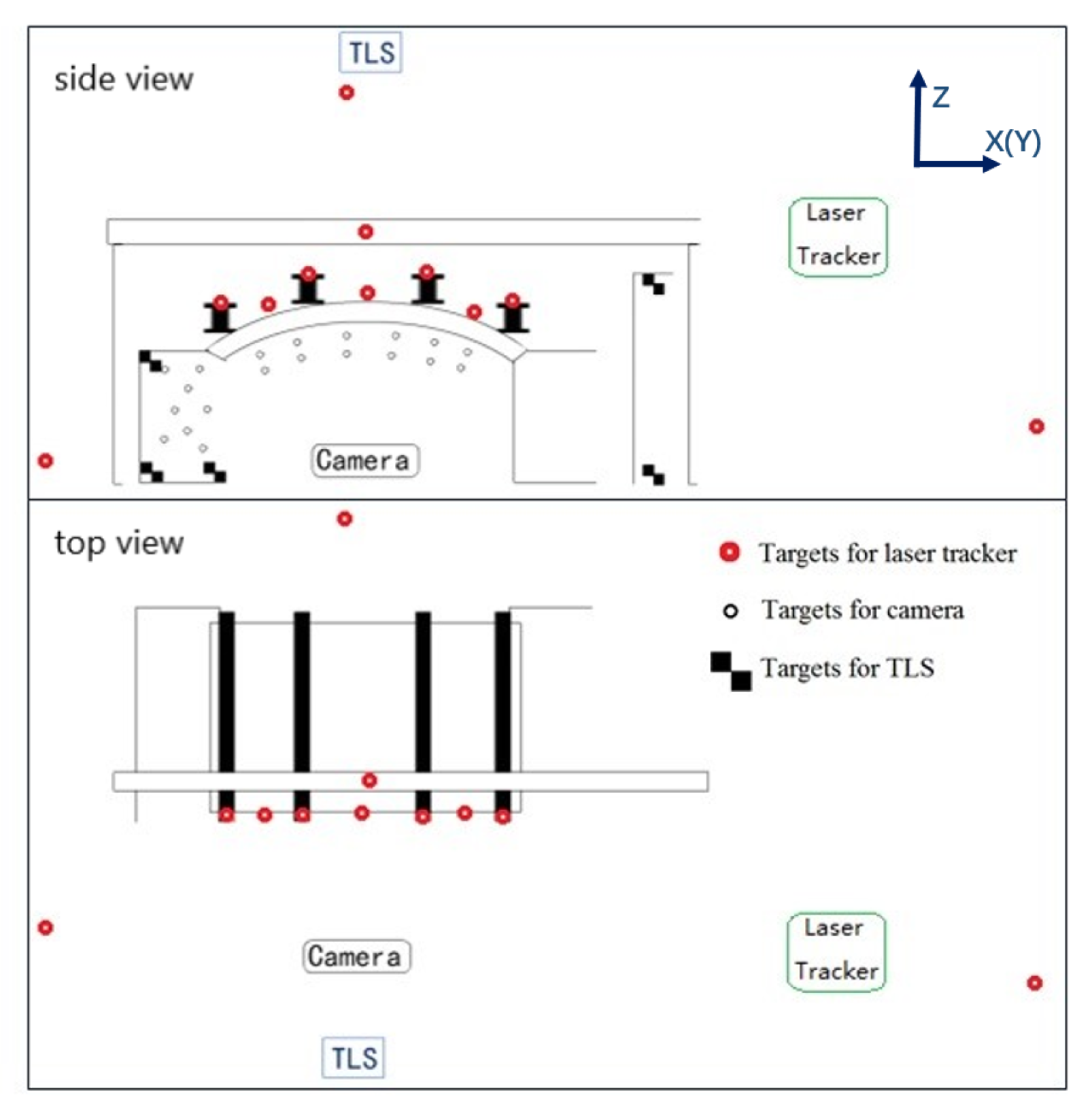
A multi-sensor-system (MSS) consisting of a TLS (here Z+F Imager 5006), laser tracker (here Leica AT960LR) and digital camera (here Nikon D750) were used to acquire the data from the deformable arch structure. The positions of the MSS relative to the arch structure are shown in Figure 1 (see also [16]). TLS data were acquired in “super high” resolution mode with normal quality. The vertical and horizontal resolution was and vertical and horizontal accuracy was rms. The TLS scanned the top and the side surfaces of the arch. The laser tracker was used as a reference sensor for the validation purpose, which allows sub-millimeter accuracy with a maximum permissible error of [26]. In addition, a digital camera was used to capture the feature points with a high resolution (thus exploiting their strength in discrete feature point extraction). Targets were mounted in the surroundings and on the arch (see Figure 1) to perform the external calibration between the sensors.
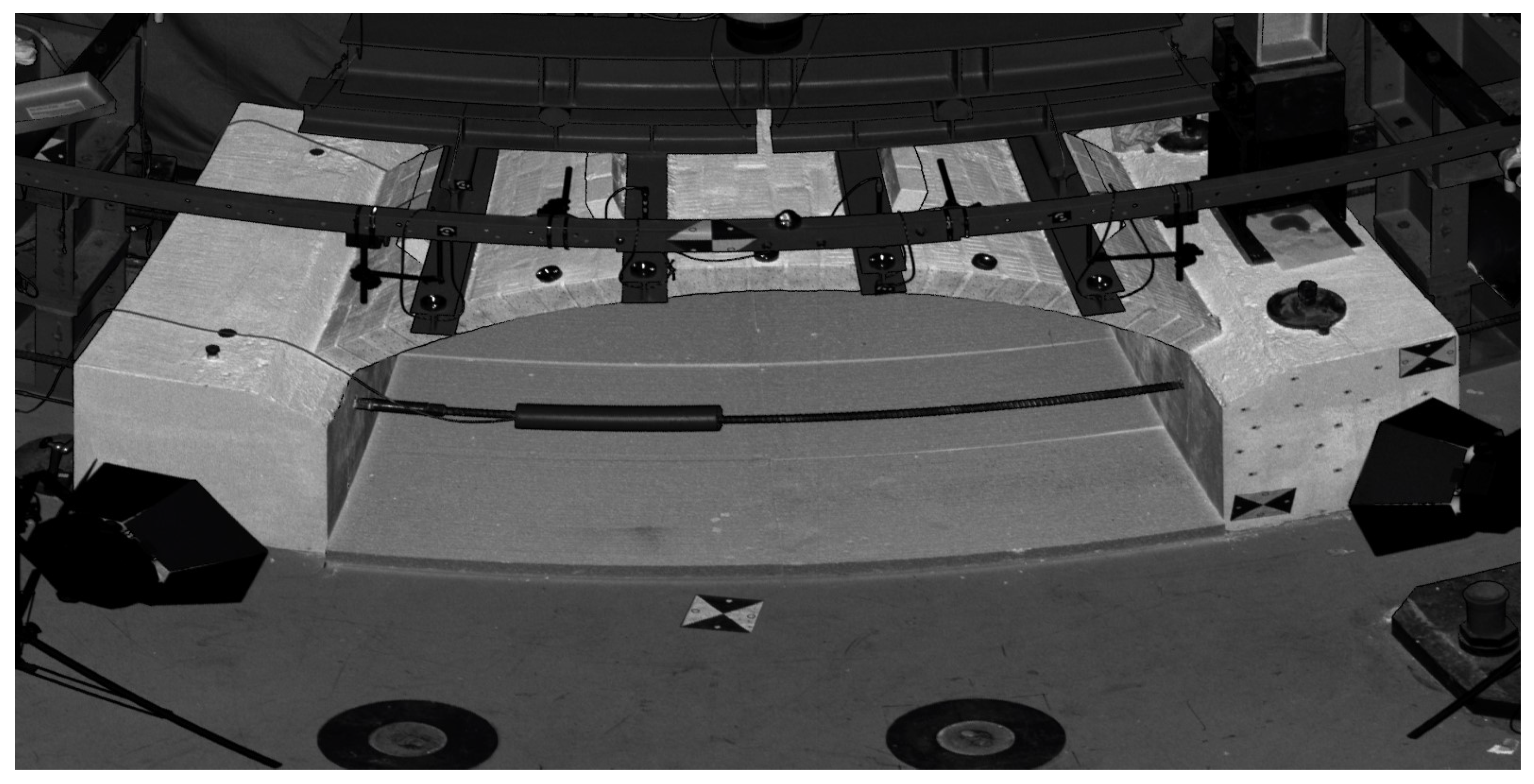
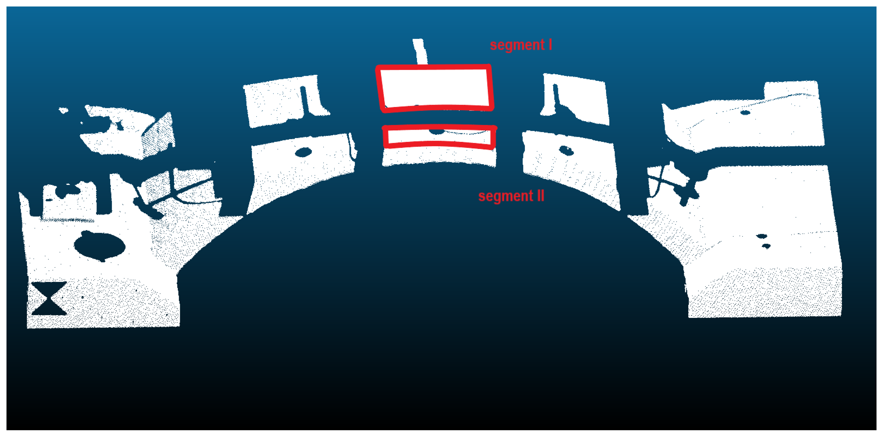
Among various datasets, the focus of this literature lies in capturing the data by the TLS to use a large number of 3D point clouds with a high accuracy in approximating a surface model, which is important in rigorous deformation monitoring. In our experiment, the top surface of the arch is of great interest since it is under load pressure in the consecutive 13 epochs and has obvious movements compared to the other parts of the structure. However, as can be seen from Figure 1, the top surface is partially occluded by the steel beams. Consequently, it is necessary to extract the top-surface points in order to enable an accurate surface model. As a preliminary step to separate the obstructions and the arch-shape part of the object, the reflectance image was generated by using the reflectivity values of the raw TLS data. It was performed by assigning the reflectivity values of each point cloud to one pixel based on the scan resolution [27] (see Figure 2). Since the occluded objects such as the beams on top of the arc shape object were darker compared to the arc shape part, it could be discarded by means of the OpenCV threshold function and by setting the threshold value manually to 80 from a range of 0–255. Therefore, those values greater than 80 were set to 0. However, before performing the thresholding, OpenCV GaussianBlur function with a size of 5 was applied to reduce the image noise. Next, the morphological opening and closing filters were applied to discard the very small segments. As previously, the position and orientation of the global coordinate system was defined in Figure 1, the Z-axis was in the zenith direction. Therefore, the Pass Through filter of the Point Cloud Library was applied to cut off those 3D point clouds below or greater than the predefined threshold in the Z-axis direction. Then the “setFilterLimits” member function of this filter was set to (−4.50 m, −3.75 m) to select the 3D point clouds within the boundaries. Subsequently, the StatisticalOutlierRemoval filter of the Point Cloud Library was applied to remove the outliers of the 3D point clouds. In this filter, the k nearest neighbor points were used to estimate the mean distance. Therefore, its “setMeanK” member function was set to 20. Next, the “setStddevMulThresh” member function of this filter was set to to reject the outliers by means of the test. The extracted arch surface data is shown in Figure 3. As an example, only two representative segments of the point cloud within the red boundary are separately investigated since the middle area has significant deviations compared to the other parts of the surface. The same methodology is applicable in modeling other segments.
2.2. Surface Approximation
In surface-based deformation analysis, an appropriate surface model is required as a representation of each deformation status. Among the various parametric models, polynomial surface fitting are the most common approach due to its easy implementation [9,16], while free-form surfaces, especially B-splines, have become relevant to deformation analysis due to their capacity to accurately model more detailed geometrical features including sharp edges, cusps, and leaps [28]. The functional relationships behind B-splines and polynomials, as two of the most commonly used types of surface model, as well as the corresponding approximation steps, are described in this subsection.
2.2.1. B-Spline Surface Approximation
The mathematical description of a 3D point
on a B-spline surface is based on the bidirectional combination of basis functions , and 3D control points , which are located on a bidirectional net with the number of and in u- and v-directions.
B-spline surface approximation builds upon B-spline curve fitting in the two directions. Following Bureick et al. [17], this procedure can be carried out in three steps:
- Parametrization of the measurements with s rows and t columns with respect to the u- and v-direction.
- Determination of the knot vectors and in the u- and v-direction.
- Estimation of the control points by means of a linear Gauss–Markov model.
The first two steps consist of the parameterization and computation of knot vectors, which serve as input parameters for the final estimation. Since the calculation of B-spline parameters are beyond the scope of this paper, the interested reader is referred to Bureick et al. [17] and Piegl and Tiller [29].
The final step of B-spline approximation is to estimate the positions of the control points, which is done essentially by adjusting a linear Gauss–Markov model (cf. [29,30]). Given measured points located on a grid defined by s rows and t columns, they also can be arranged in matrix form as
The addition of a corresponding matrix of residuals to the observation matrix yields the adjusted observations, which can be represented by the functional B-spline model in Equation (1). We thus have for a particular observation the equation
where and . We can write all of the equations jointly in the form with a design matrix within which the basis functions , are calculated based on the parameterization and knot vectors
and (unknown) parameter matrix . We assume all of the measured point coordinates to have identical accuracies and to be uncorrelated, so that we obtain for the least squares estimates of these parameters:
2.2.2. Polynomial Surface Approximation
Denoting a generic surface point by , the Z-component can be expressed as the two-fold linear combination
where is the coefficient vector having elements, and where p and q represent the polynomial degrees with respect to the X- and Y-components, respectively.
Polynomial surface fitting consists of the estimation of the coefficient vector , which we carry out again in the least-squares sense by minimizing the sum of squared (“vertical”) residuals
where is now an observation vector consisting of the N measured Z-coordinates. The design matrix
is computed by exponentiation (where , ) and multiplication of the X- and Y-components, which are considered as error-free. Under the assumption again of homoskedastic and uncorrelated measurements, the estimated parameters are given by
2.2.3. Parameter Number of Competing Models
The approximation quality of a surface model is related to its complexity embodied in the number of parameters. Hence, when choosing pairs of models to be compared, we should pay attention to the parameter numbers.
In the initial comparison, the target segments of the point cloud of the first epoch are modeled by means of polynomial and B-spline surface functions with similar numbers of parameters in order to minimize the effect of model complexity. As the most basic description of a surface, the second degree polynomial function () with six unknown parameters is approximated. A B-spline surface with the same parameter number (, ) is modeled as a competitor. In order to facilitate a comprehensive analysis, polynomial functions of higher degrees are adjusted and compared to other estimated B-spline surface models. According to the general polynomial model Equation (6), a third-degree polynomial model is based on the specification of , resulting in 10 unknown parameters to be estimated. It is reasonable to compare this model with the adjusted B-spline surface involving nine parameters (). Further comparisons are carried out between the fourth-degree polynomial and B-spline surface models with 15 and 16 unknown parameters, respectively. Table 1 lists the candidate surface models mentioned above, where and represent the number of parameters of the polynomial and of the B-spline models, respectively.
It should be mentioned that polynomial functions of degrees higher than four are useless in our numerical example, since the resulting normal equation matrices within parameter estimation Equation (9) would be ill-conditioned. In this case, on the one hand, it is quite interesting to compare the best-fitting fourth-degree polynomial model with a higher-quality yet more complex B-spline surfaces when considering the complexity of models as penalization. It is predicted that the latter would be superior to the former in initial comparison pairs, but the superiority is expected to be offset by penalization due to increasing parameters. The comparison results of Segment I will be presented in Section 3.1 in Table 3 and in Appendix in Table A1. It helps to judge in which situation the B-spline models are recommended compared with the polynomial model. On the other hand, in practice, among the recommended B-spline models, we need the optimal one for further deformation analysis, which motivates the comparison within B-spline models. The comparison results of Segment I will be shown in Section 3.2 in Table 5 and in Appendix in Table A2.
2.3. Model Selection Method
The aim of model selection is to find a balance between the parsimony of the model and its approximation quality [21]. Unlike the trial-and-error procedures and information theoretic criterion model selection approaches, we adopt the likelihood-ratio-based hypotheses testing framework to discriminate between the competing models. The likelihood ratio tests are generally used to compare two nested models; however, in our case, the polynomial surface model and B-spline model are non-nested because neither model can be reduced to the other by imposing a set of parametric restrictions or limiting process.
Regarding the non-nested models selection problem, in Cox [23] and Vuong [25], the authors proposed respective approaches to extend the likelihood ratio test into non-nested cases. In this subsection, both a simulation-based version of Cox’s test and Vuong’s test, which will be instantiated later with the experiment data, are explained.
2.3.1. Simulation-Based Version of Cox’s Test
Under the assumption of normally distributed, uncorrelated and homoskedastic random deviations, the observation models can be defined in terms of the generic log-likelihood function
where the variance factor is treated as an unknown parameter alongside the functional parameters. Let us define , and to be the specific log-likelihood functions with respect to the design matrices Equations (4) and (8), respectively. Both types of design matrix define different types of functions where neither is a special case of the other one. Thus, the two sets of multivariate normal distributions defined by and are non-nested, so that the likelihood ratio test cannot be applied in its usual form ([31] cf.) (pp. 276–278).
According to Cox [23], we may, however, use the logarithmized likelihood ratio
for testing the adequacy of the polynomial model against the B-spline model. Note that the substituted least squares solutions Equations (5) and (9) are identical to the maximum likelihood estimates; furthermore, the two occurring maximum likelihood estimates of the variance factor are given by and ([31] cf.) (pp. 161). The statistic follows approximately a normal distribution
- with certain expectation and standard deviation if the polynomial model is true, and
- with certain expectation and standard deviation if the B-spline model is true.
Thus, we may calculate the approximately standard normally distributed statistics and for carrying out two separate tests of the hypotheses—
- the polynomial model is true;
- the B-spline model is true—
at significance level . We may determine the means and as well as the standard deviations and conditionally on the two parameter solutions , and through a Monte Carlo simulation in analogy to the approach taken in Williams [24].
According to that approach, we start by generating a large number M of observation vectors , …, randomly from the N-dimensional Gaussian distribution . Based on these samples, we compute the corresponding solutions , …, with respect to the polynomial model and , …, with respect to the B-spline model. We use the first solution set to evaluate the corresponding log-likelihood functions , …, , and the second set to evaluate , …, , so that we may compute the realizations , …, of Equation (11). Thus, the arithmetic mean and empirical standard deviation of these sampled logarithmized likelihood ratios serve as estimates of and , leading to the standardized Gaussian test statistic under the currently assumed polynomial model.
The second test statistic (with respect to the test of the B-spline model) is computed in analogy to the first one, sampling now M observation vectors from , and using the two new sets of parameter solutions (regarding the polynomial and B-spline model) to compute the M realizations of the log-likelihood ratios, as well as the resulting estimates of and .
Since Cox [23] suggests applying the one-sided decision rules,
- reject if , and
- reject if
(where is the -quantile and the -quantile of the standard normal distribution), the execution of the two tests may result in four mutually exclusive decisions:
- The polynomial model is rejected and the B-spline model is not rejected in the case of
- The B-spline model is rejected and the polynomial model is not rejected in the case of
- Both the polynomial and the B-spline models are rejected in the case of
- Neither the polynomial nor the B-spline model is rejected in the case of
2.3.2. Vuong’s Non-Nested Hypothesis Test
Vuong’s test is based on the Kullback–Leibler information criterion (KLIC), which measures the closeness of two models and uses the likelihood-ratio-based statistics to test the null hypothesis that the competing models are equally close to the true data generating process against the alternative hypothesis that one model is closer [25]. Specifically, the two competing models are given as and , l denotes variables, and and are their respective parameters. As defined by Vuong, the two models’ Kullback–Leibler distances from the true density are and , respectively, where denotes the expectation under the true model, and and are the pseudo-true values of and . It is clear that the model with a minimum KLIC value is closer to the truth, which is, however, hard to quantify. Thus, an equivalent selection criterion can be based on the quantities and , the better model being the one with larger quantity.
There are three possible cases when comparing, and we propose the null hypothesis, as the two models have equal expectation values so that they are equivalent. One alternative hypothesis is , which means is the better model. The other alternative hypothesis is , meaning is better. Since the quantity is still hard to quantify, Vuong consistently estimates it by times the likelihood ratio statistic.
In our specific case to discriminate between the polynomial and B-spline surface models, with independent and identically distributed observations , the probability density functions of competing models are given as and , in which the parameter matrix is estimated in its respective Gauss–Markov models and the variance factor for competing models is calculated in the same way as in Cox’s test: and . Thus, we propose the hypothesis in discriminating between models as follows:
- : the polynomial and B-spline models are equally close to the truth;
- : the polynomial model is better since it is closer to the truth than the B-spline model is;
- : the B-spline model is better since it is closer to the truth than the Polynomial model.
Similar to Cox’s test, the statistic of Vuong’s test is also based on likelihood ratio. If we define and as log-likelihood functions for competing polynomial and B-spline surface models, the logarithmized likelihood ratio is calculated as (11). Vuong’s test is potentially sensitive to the number of estimated parameters on condition that the logarithmized likelihood ratio is adjusted by a correction factor K.
Vuong [25] suggests that K corresponds to either Akaike’s information criteria (AIC) or Bayesian information criteria (BIC). According to the former, , and, according to the latter, , where and are numbers of parameters in competing models. The BIC generally penalizes free parameters more strongly than AIC. Here, we prefer the BIC correction factor in order to avoid an over-fitting problem.
Then, the adjusted likelihood ratio is rescaled in statistic as , where is the variance calculated as
According to Vuong [25], when N is reasonably large, the statistic converges, asymptotically to a standard normal distribution, . In the decision-making process, practically, we compare against the quantiles of a standard normal distribution, , for significance level . The models are discriminated through the following decision rules:
- The polynomial and B-spline models are equally close to the truth in case of
- The polynomial model is better since it is closer to the truth than B-spline model in case of
- The B-spline model is better since it is closer to the truth than Polynomial model in case of
2.4. Deformation Analysis
To probe the selected surface model’s performance in deformation analysis, each target segment of the 1st and 13th epochs are approximated by surface models. In the specific application, loads were exerted perpendicular to the ground (in the Z-direction) so that the deformation () is defined as the difference in approximated Z-coordinates of the two epochs (, ), that is,
The evaluation criterion of surface models’ performance is whether they are able to reflect the actual deformation, which are recorded by the point cloud. Since it is impossible to get an exact mutual spatial referencing of points in the different epochs, we compared the point clouds through the block-mean approach used in Paffenholz et al. [32]. In this application, the blocks had a size of 5 mm × 5 mm involving 2–9 points, for which the medians of the Z-coordinates were computed as representative values. The high-density block-means between the two epochs were used to approximate the point-wise changes.
3. Results
3.1. Evaluation of Competing Polynomial and B-Spline Models
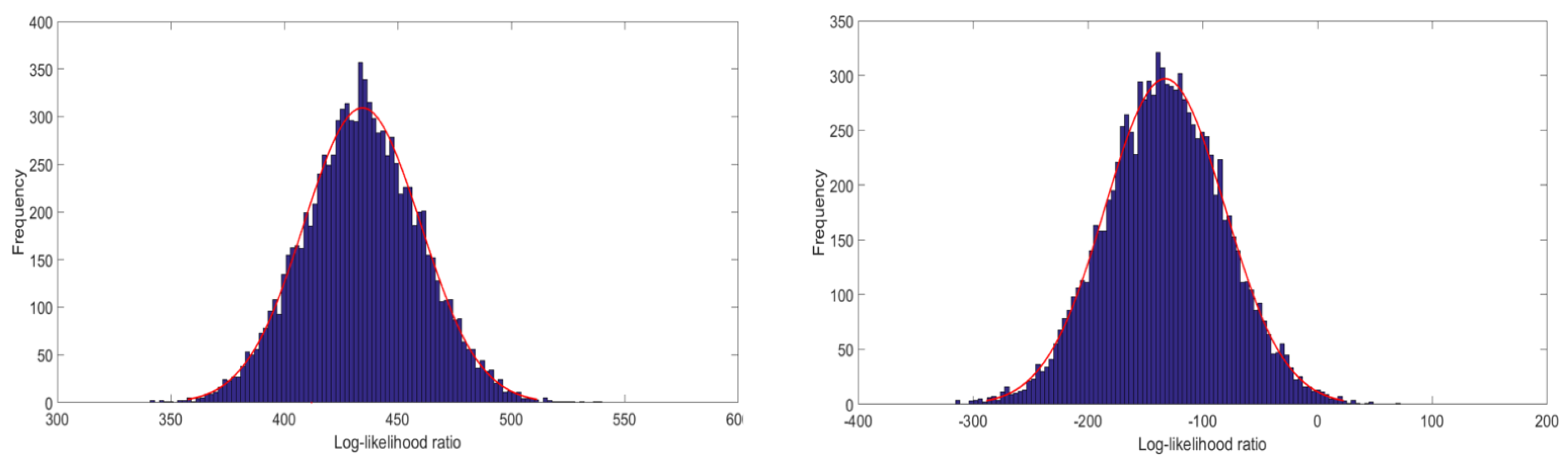
In order to statistically discriminate between the aforementioned polynomial and B-spline surface models listed in Table 1, the result of Cox’s and Vuong’s test for the two segments are given in Tables 2 and 4, respectively. It is noticeable that the observations are assumed to be following identical and independent normal distribution, which satisfy the prerequisite of both tests. In addition, Figure 4 demonstrates that the 10,000 log-likelihood ratio values of Equation (11) sampled with respect to Cox’s test follow approximately a Gaussian distribution under both the polynomial and B-spline surface models. Thus, it is justified to standardize the log-likelihood ratio computed from the actual measurements by means of the sample mean and standard deviation under each of the two stochastic models (resulting in the values for and shown in Tables 2 and 4).
The statistics are compared to the critical value at type-I error rate . In Cox’s test, the critical values are for statistic , and for statistic . In Vuong’s test, the critical values are and .
It can be clearly seen in Table 2 that, within the first pair of models, the B-spline surface model with six parameters is preferred over the second-degree polynomial model, since, in Vuong’s test, the former is better verified, and, in Cox’s test, the latter is rejected. This result indicates, with minor parameters, B-spline models are superior to the equivalent polynomial one. This conjecture is validated. In the second pair of models, neither the third-degree polynomial model nor the B-spline model is rejected or selected by tests, whose findings indicate that there is no significant difference between the two models. Next, further comparisons are carried out within Pair III between a fourth-degree polynomial and B-spline models with 15 and 16 unknown parameters, respectively. According to the tests results, Vuong’s test indicates there is no significant superiority between the two, while the polynomial model is rejected by the Cox’s test.
As mentioned before, polynomial functions of degrees greater than four become numerically unstable due to the appearance of singular matrices, so that they cannot be recommended. By contrast, approximated B-spline surface models for Segment I can describe the target segment of the point cloud increasingly well when the parameters are increased, without producing such numerical difficulties. When comparing the increasingly accurate B-spline models with the fourth-degree polynomial surface model of Segment I by means of both hypothesis tests, as previous predicted, we find that the Cox’s test always rejects the models with fewer parameters, which leads to the problem of over-fitting. By contrast, Vuong’s test initially tends to prefer B-spline models due to higher approximation quality until Pair 36, in which large quantities of parameters are set (). Table 3 offers the last five comparison pairs to show the aforementioned change in test decision. The complete test results for discriminating between fourth-degree polynomial and B-spline surface models are shown in Table A1.
The testing results for Segment II are listed in Table 4. It is indicated by the first comparison pair that both the polynomial and the B-spline surface models are rejected by Cox’s test, while Vuong’s test considers the polynomial model to be closer to the truth than its competitor. Within the second and third pairs, B-spline models are judged as insufficient by Cox’s test, whereas the polynomial models are preferred by Vuong’s test.
The testing result differs greatly between the two segments. These differences can be explained by the fact that Segment II contains large data gaps, which substantially distort the B-spline model estimation, in contrast to the polynomial model estimation.
3.2. Evaluation of Competing B-Spline Models with Various Parameters
The results in Table 3 motivate us to evaluate B-spline surface models with increasing parameters by means of Vuong’s test in search of a balance between model complexity and its approximation quality. Two B-spline models with different degrees or control points (Model I and Model II) are non-nested because the parameters in Model I are not a subset of the parameters in Model II. The modification of the degree or the number of control points (see Equation (1)) leads to a change in the number of knots, resulting in different basis functions. The comparison of pair setting and evaluation results are shown in Table A2, where denotes the parameter number of the first B-spline model and denotes that of the second model in the competing pair. The statistic value and test decision are shown in the last two columns. Here, we present the comparison results of B-spline models with and () instead of neighbor models (, ). There were large oscillations in the testing results of the pairwise neighbor models. These oscillations, which were due to the similar parameter number and model quality between neighbor models, served as noise and would confuse the result. The testing results became stable when we chose comparison models as and .
According to the results in Table A2, B-Spline Model II with more parameters is preferred initially; however, due to the increasing penalized term, B-Spline Model I is preferred in the final pair. The middle comparison pairs are considered to be in the overlapping region, where the test decisions swing between the two competing models. Table 5 shows the comparison pairs in the overlapping region. It can be considered that the balance sought of the model’s complexity and its approximation quality is located in this region. Figure 5 offers a direct view of test statistic in comparison with critics boundaries and .
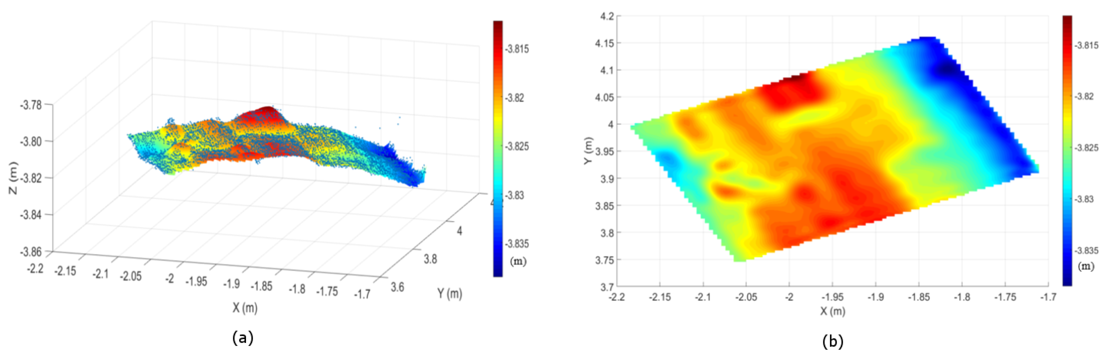
We consider the B-spline model with 361 parameters (), which lies roughly in the middle of the overlapping region, as the optimal one. Figure 6 shows the side- and top-view of this surface model.
3.3. Performance in Deformation Analysis
3.3.1. Deformation of Segment I
According to the model evaluation results for Segment I, the fourth-degree model is best-fitting among polynomial surface models, while the B-spline surface model with 361 parameters is optimal among all candidate models. We approximate both types of surface models for the point cloud in the 13th epoch with the same number of parameters.
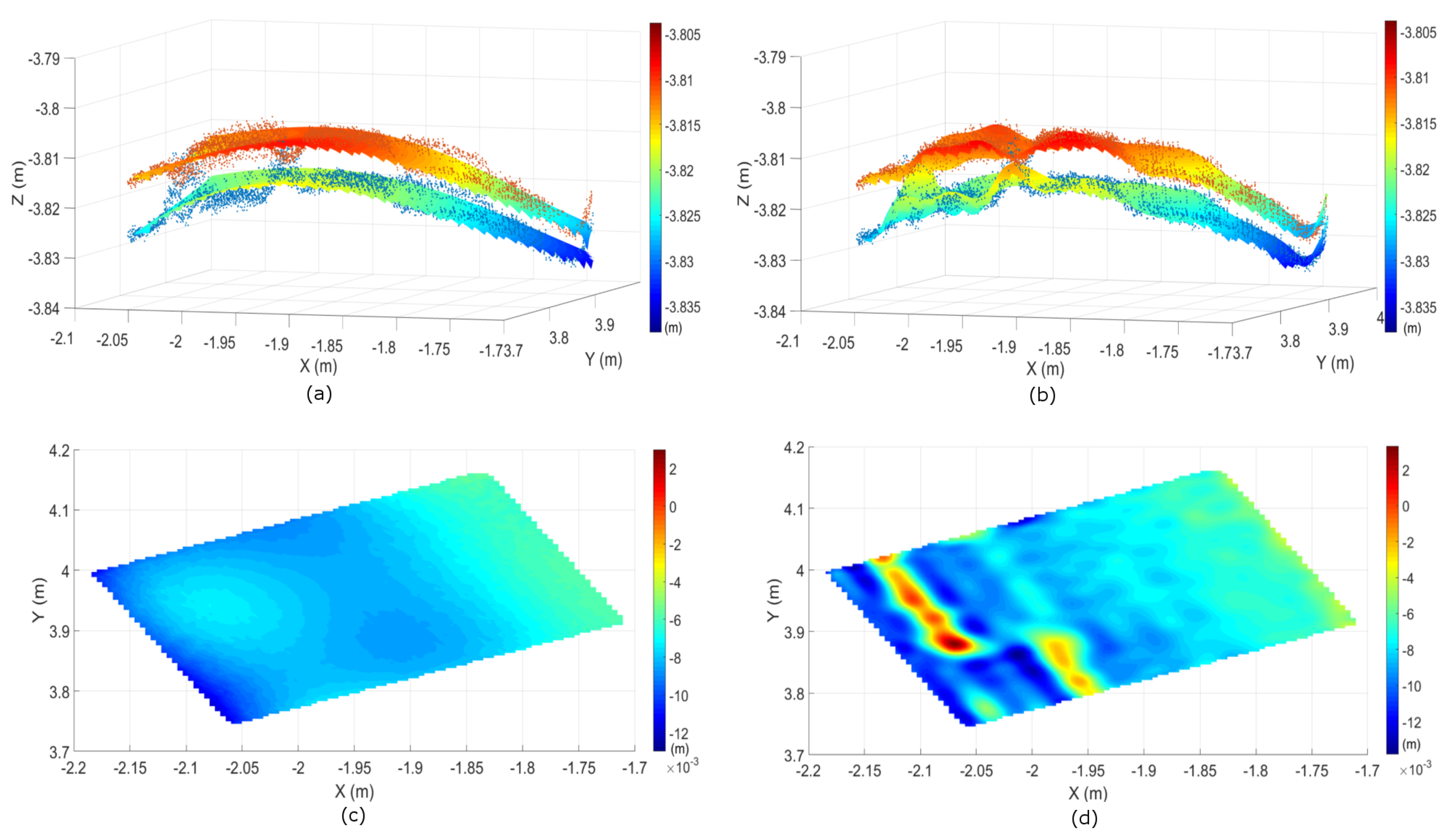
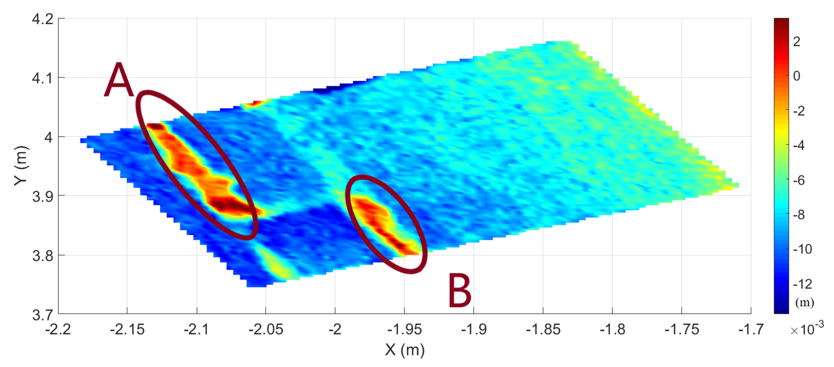
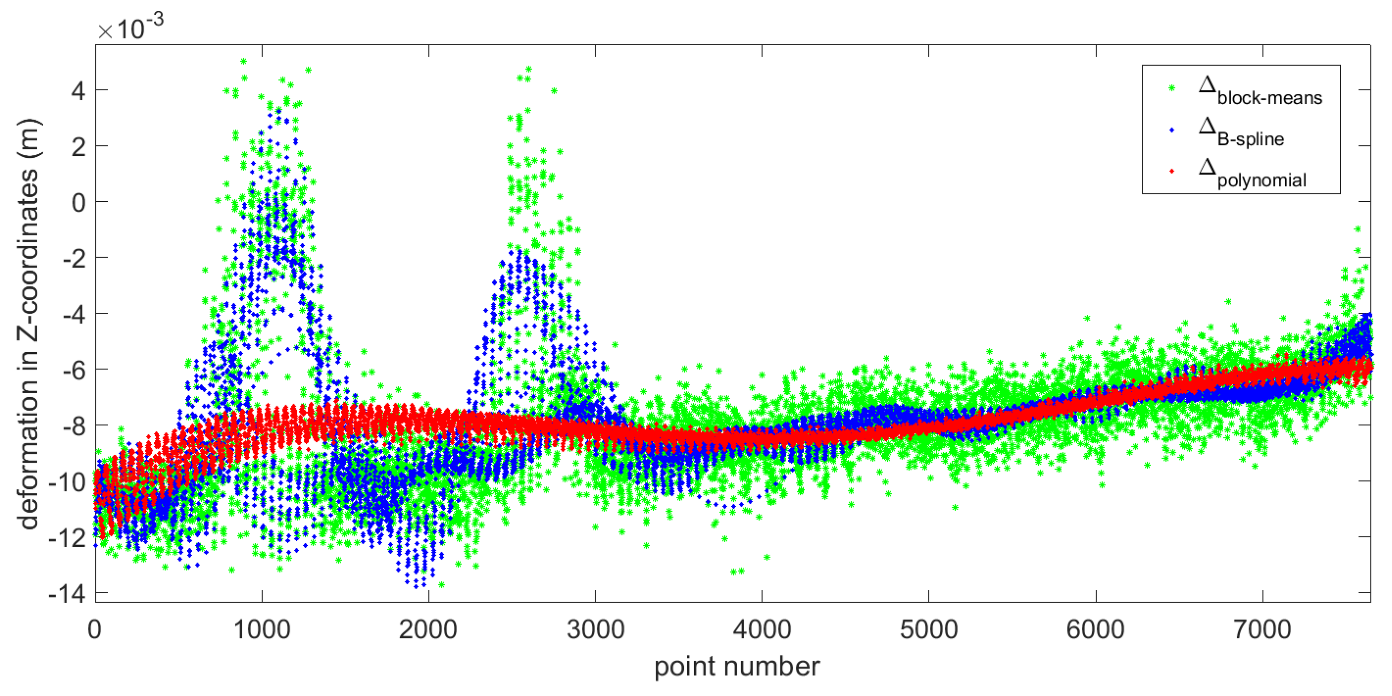
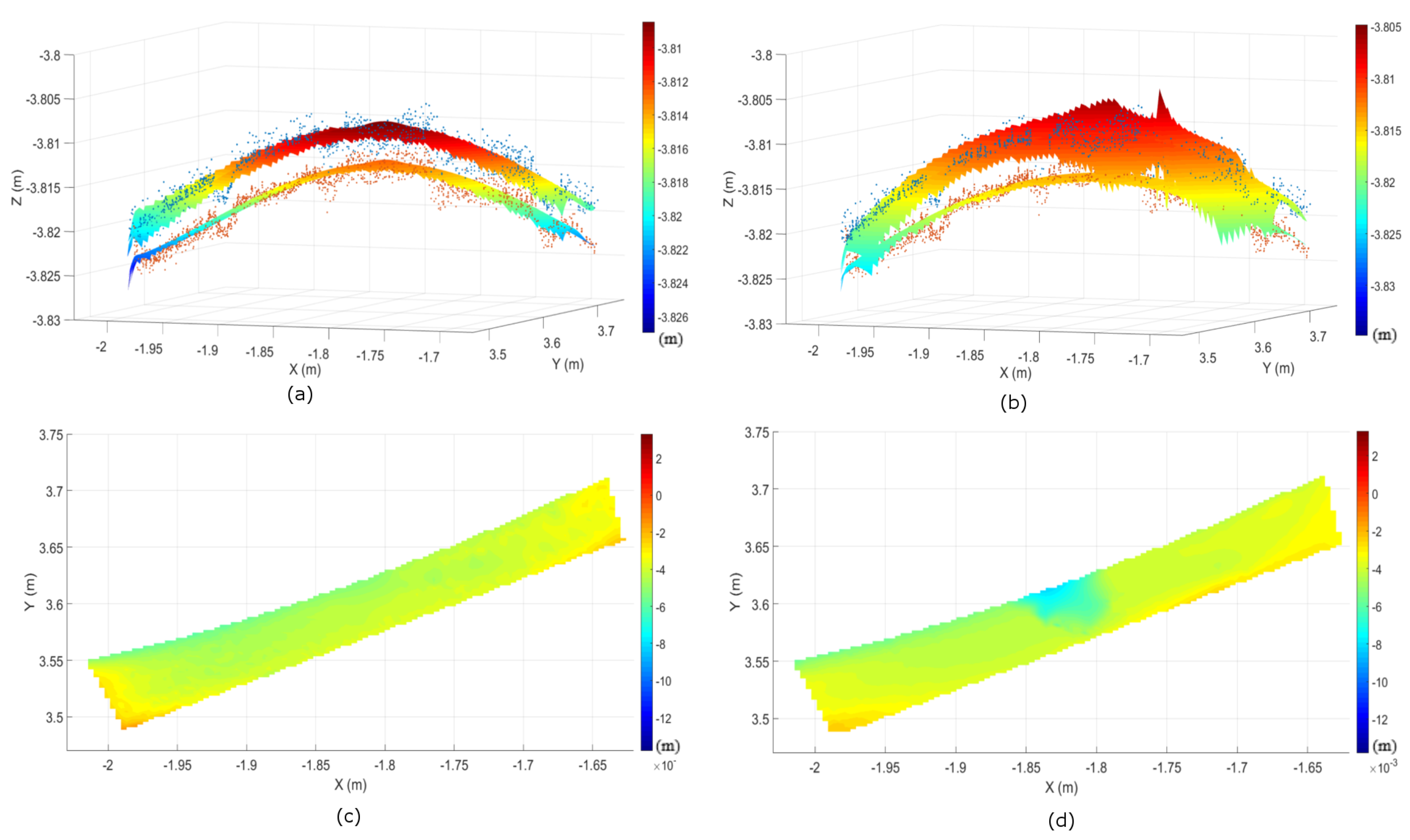
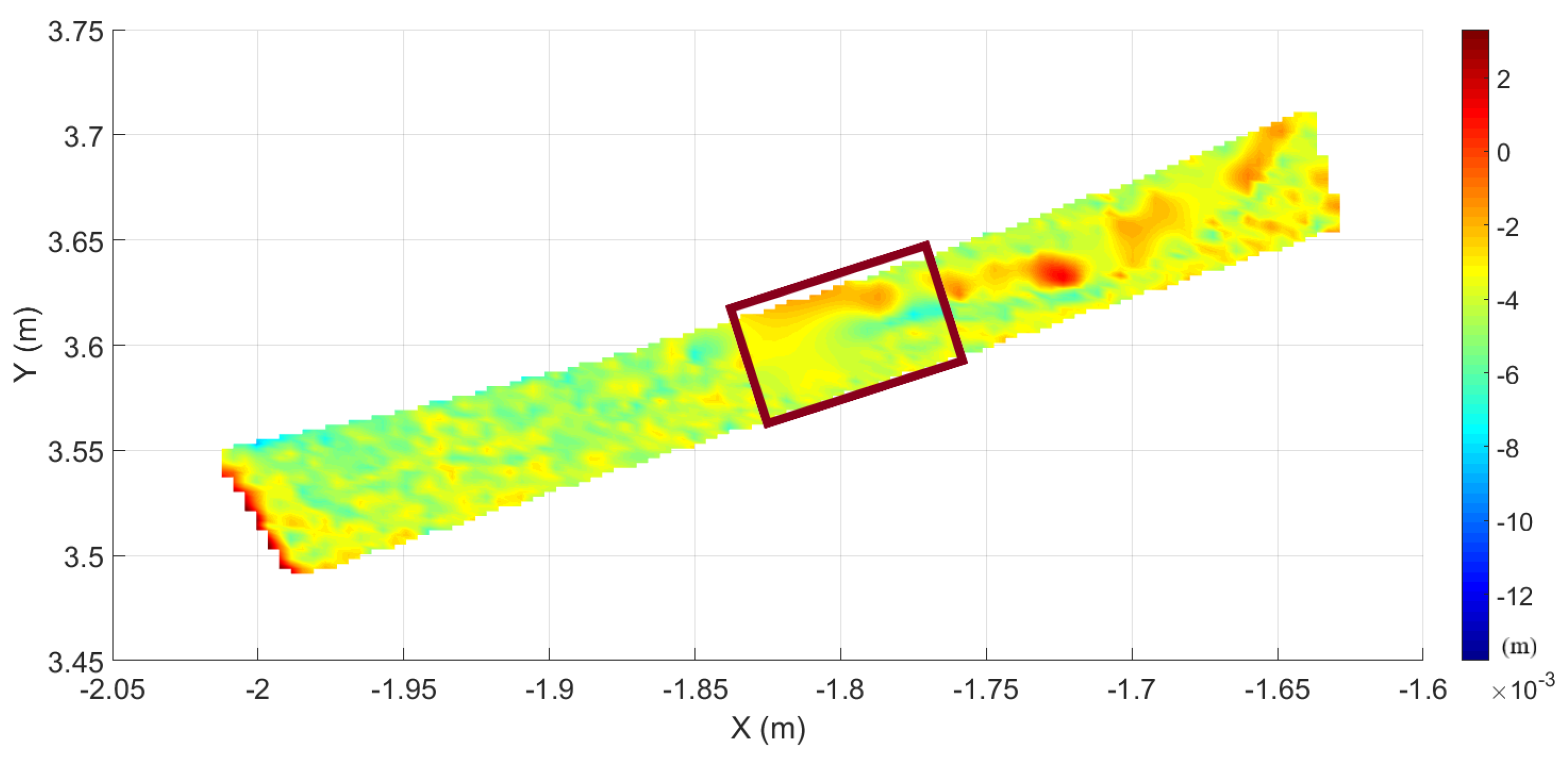
Because traditional polynomial models are still the most widely used regression method in deformation analysis due to their simple operating, while the B-spline model has the potential to describe geometrically complicated objects, it is of significance to compare the performance in this numerical example between two surface models with their best-fitting parameters in reflecting deformation. In Figure 7a shows the modeled fourth-degree polynomial surfaces for the 1st (upper) and 13th (lower) epochs, while Figure 7b shows the equivalent epochs approximated by means of B-spline surfaces with 361 parameters. It is obvious that the B-spline surfaces in Figure 7b describe more detailed geometrical features than polynomial model in Figure 7a. The arch’s deformation in Z-coordinates between the two epochs are shown in Figure 7c,d, by means of approximated polynomial surfaces of Figure 7a and B-spline models of Figure 7b, respectively. In order to validate that the reflected changes are the real arch’s deformation recorded by the points instead of regression models, we compare the two epochs’ point cloud through the block-mean approach (see Figure 8 for the differences between the two epoch’s point clouds). By comparison, it is obvious that the deformation shown in Figure 7d for B-spline models reflect these differences precisely, especially in Areas A and B; in contrast, the fourth-degree polynomial surfaces in Figure 7c fail to show this deformation due to their global smoothing effect. The preceding difference and model deformation are also shown pointwise in Figure 9. The green asterisks denote the point-wise differences recorded by block-means, while the red and blue asterisks are that reflected by the fourth-degree polynomial and B-spline surfaces, respectively.
3.3.2. Deformation of Segment II
In Figure 10a shows the modeled fourth-degree polynomial surfaces for the 1st (upper) and 13th (lower) epochs, while Figure 10b shows the same epochs approximated by means of B-spline surfaces with 16 parameters.
The missing data lead to oscillation, especially at the edges of the data gap (see the bounded area in Figure 11). Thus, it can be found from Figure 10d that the deformation reflected by B-splines is far from the truth. Here, the estimated B-spline surfaces clearly show the aforementioned numerical instabilities, which are caused by an inadequate specification of the knot locations with the applied classical approach to knot vector determination in Piegl and Tiller [29].
4. Discussion
In our numerical example of Segment I, the different results between the two hypothesis tests are caused by the penalized term regarding the parameter numbers. In Table 2, for example, Pair III has various test results. In Cox’s test, the fourth-degree polynomial model is rejected because of the relatively poor accuracy, while the Vuong’s test result recommends neither, because the improved accuracy is offset by the punishment of increasing parameters. In parallel, in Table 3, the test decision initially shows in the consistency of both tests that the B-spline models are better compared to the fourth-degree polynomial model. However, as the number of parameters increase, the improvement of model accuracy declines. Finally, in Voung’s test, the advantage of the model’s quality is offset again by the large penalized value and, consequently, shows results that are different from Cox’s test in Pair 36.
Although Cox’s test without penalized term is limited to discriminate models with similar parameters, it is practically very straightforward to implement and are able to offer more reliable decisions by simulating the test distribution, especially when the sample size is small [33]. We expect to improve the simulation-based version of Cox’s test by adding a proper correction factor similar to that in Vuong’s non-nested hypothesis test, which would be one of our future research projects.
Since previous geodetic literatures [21,22,28] has solved the model selection problem through well-known penalization information criteria: the AIC and BIC, it is necessary in this section to compare Vuong’s non-nested hypothesis test with this widely used approach. It is noticeable that there are close connections between AIC, BIC, and Vuong’s test. Taking the BIC as an example, the value of model 1 is calculated as
where is the maximum value of the likelihood function for Model 1, denotes the parameter quantity, and N is the number of measurements. The different BIC value between two models is calculated as
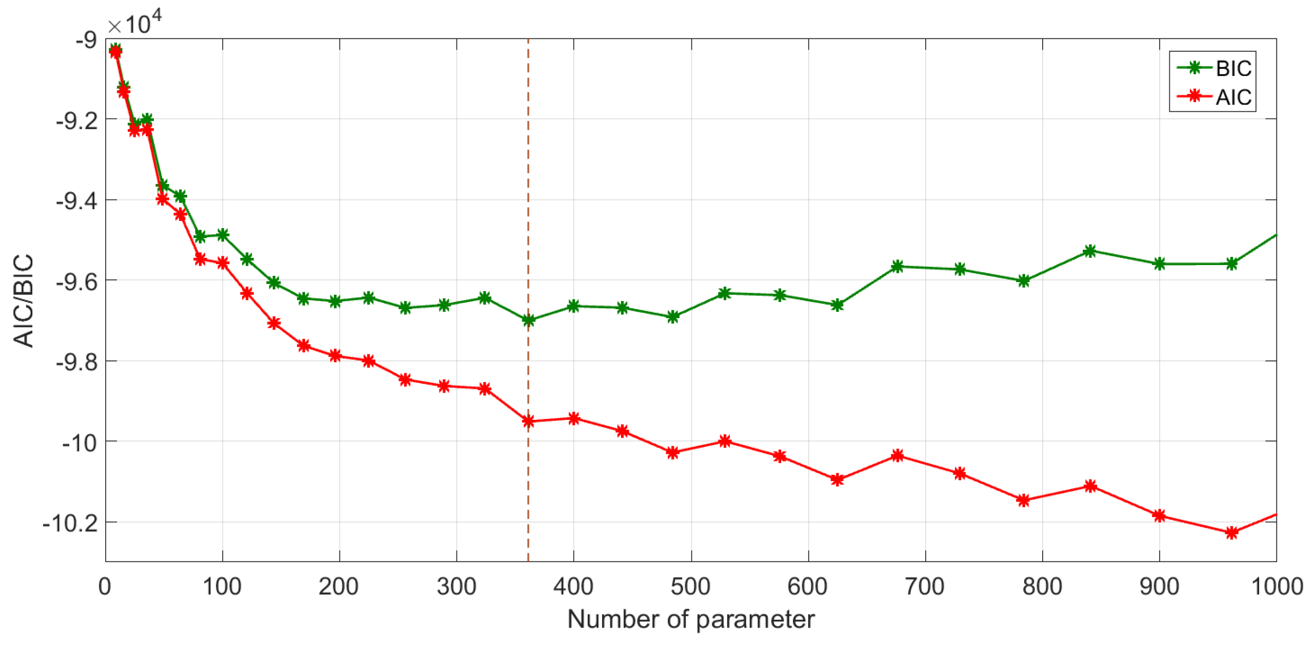
where the first term in the right part contains logarithmized likelihood ratio in Equation (16), so that is equal to the (un-normalized) adjusted test statistic for Vuong’s test. The main difference is that Vuong’s test makes judgments in a framework of likelihood ratio hypothesis testing, which offers the advantage that significant probabilistic differences between models can be detected, which is not provided by classical penalization information criterion methods. We compared the Vuong’s test results with both the AIC and BIC to discriminate between B-spline surface models, and the result is shown in Figure 12. According to the BIC’s curve, the B-spline model with 361 parameters (n = 18, m = 18) is optimal, since it is associated with the smallest value. This result is quite consistent with the judgment of Vuong’s test, because the BIC penalized term is used in our adjusted test statistic. By contrast, the AIC tends to prefer much larger models.
Furthermore, the performance of best-fitting polynomial and B-spline surfaces in reflecting deformation were compared. The superior model was the one able to reflect the deformation details recorded by the point clouds. In order to get an exact mutual spatial referencing of points in the different epochs, we used the block-mean approach to approximate the point-wise changes. The comparison results of Segment I indicated that the selected B-spline surfaces can reflect the actual deformation, especially in Areas A and B of Figure 8, while the best-fitting polynomial model failed to offer this information due to its global smooth effect. However, in the case of Segment II, B-spline models failed to reflect the actual deformation values, especially at the edges of the data gap.
5. Conclusions
In this paper, we approximated point cloud data of a surveyed arch structure by two common surface models: polynomials and B-splines. Subsequently, we compared different adjusted surface models via Cox’s test and Vuong’s test to select an appropriate parametric model, which was sufficient to describe the geometrical features of the two target segments.
Regarding Segment I, in the initial comparison between lower degree polynomial and B-spline models, none of the B-spline models investigated was rejected, but only the polynomial model with degree 3 was found to be adequate in Cox’s test, while Voung’s test indicated no significant difference in Pairs II and III. However, none of these models could reflect detailed geometrical features of target segments. Since it was not possible to increase the degree of polynomial approximation (due to numerical instability of the normal equations) for modeling geometrical details, B-splines were recommended in the field of applications presented. That motivated us to search for an optimal model balancing between approximation quality and its complexity. According to Voung’s test decisions, the B-spline surface model with was considered as the optimal one in the specific numerical example.
The model selection testing results of Segment II were quite different from that of Segment I. All the B-spline models were rejected by Cox’s test, while in Pairs II and III, the equivalent polynomial surfaces were preferred by Voung’s test, as a consequence of the aforementioned numerical instabilities with the knot vector determination and the resulting oscillation effects. Such deficiencies were clearly reflected by the model selection tests, which rejected inadequate B-spline models.
A consistent model selection result was obtained by comparing Vuong’s test decision with the widely used BIC in discriminating B-spline surface models. Thus, it is concluded that the alternative model selection methodology elaborated in this paper, in parallel with well-known penalization information criteria, can effectively guide practitioners in selecting a parsimonious and accurate model for structures, such as the arch in the numerical example presented. The main difference is that Vuong’s test makes judgments in a framework of likelihood ratio hypothesis testing, which can detect the significant probabilistic differences between models. It was proved here that the models selected by the model selection tests have good performance in reflecting actual deformation.
The model selection methodology is applicable not only to TLS data but also to point clouds obtained by other LiDAR technology, such as airborne laser scanning and mobile laser scanning. There are also distribution-free hypothesis tests, such as Clarke’s test [34], available for mixed distribution observations.
Acknowledgments
The publication of this article was funded by the Open Access fund of Leibniz Universität Hannover.
Author Contributions
Xin Zhao conducted the statistical analysis and wrote the manuscript; Boris Kargoll contributed to the analysis approach and provide advice with respect to the manuscript; Mohammad Omidalizarandi contributed to the data processing; Xiangyang Xu helped to conceive the study and motivate the paper; Hamza Alkhatib organized the study and commented on the manuscript.
Conflicts of Interest
The authors declare no conflict of interest.
Abbreviations
The following abbreviations are used in this manuscript:
| AIC | Akaike information criterion |
| BIC | Bayesian information criterion |
| KLIC | Kullback-Leibler information criterion |
| MSS | multi-sensor-system |
| RMSD | root-mean-square deviation |
| TLS | terrestrial laser scanning |
Appendix A

Table A1.
Results for Segment I of Vuong’s test and Cox’s test for discriminating between fourth-degree polynomial and B-spline surface models at type-I error rate .
Table A1.
Results for Segment I of Vuong’s test and Cox’s test for discriminating between fourth-degree polynomial and B-spline surface models at type-I error rate .
| Pair | Competing Models | Cox’s Test | Vuong’s Test | |||||
|---|---|---|---|---|---|---|---|---|
| Polynomial | B-Spline | Rejected | Rejected | Preferred | ||||
| 1 | −96.88 | polynomial | −6.31 | no | −14.92 | B-spline | ||
| 2 | −82.69 | polynomial | −5.30 | no | −14.59 | B-spline | ||
| 3 | −210.65 | polynomial | −17.54 | no | −13.99 | B-spline | ||
| 4 | −324.26 | polynomial | −19.77 | no | −13.37 | B-spline | ||
| 5 | −306.37 | polynomial | −31.21 | no | −12.58 | B-spline | ||
| 6 | −323.49 | polynomial | −28.37 | no | −12.75 | B-spline | ||
| 7 | −338.20 | polynomial | −33.64 | no | −13.23 | B-spline | ||
| 8 | −359.43 | polynomial | −38.19 | no | −11.79 | B-spline | ||
| 9 | −325.74 | polynomial | −42.33 | no | −10.44 | B-spline | ||
| 10 | −341.49 | polynomial | −41.76 | no | −9.68 | B-spline | ||
| 11 | −294.75 | polynomial | −48.19 | no | −11.53 | B-spline | ||
| 12 | −333.69 | polynomial | −50.22 | no | −10.59 | B-spline | ||
| 13 | −279.57 | polynomial | −46.54 | no | −11.23 | B-spline | ||
| 14 | −318.33 | polynomial | −51.20 | no | −10.02 | B-spline | ||
| 15 | −317.28 | polynomial | −52.92 | no | −9.90 | B-spline | ||
| 16 | −275.54 | polynomial | −59.22 | no | −7.43 | B-spline | ||
| 17 | −276.37 | polynomial | −52.10 | no | −8.55 | B-spline | ||
| 18 | −313.79 | polynomial | −66.44 | no | −9.12 | B-spline | ||
| 19 | −262.48 | polynomial | −54.70 | no | −7.99 | B-spline | ||
| 20 | −270.20 | polynomial | −56.54 | no | −10.10 | B-spline | ||
| 21 | −285.65 | polynomial | −49.27 | no | −6.99 | B-spline | ||
| 22 | −268.69 | polynomial | −68.30 | no | −10.59 | B-spline | ||
| 23 | −267.04 | polynomial | −62.88 | no | v8.99 | B-spline | ||
| 24 | −241.21 | polynomial | −67.39 | no | −9.54 | B-spline | ||
| 25 | −268.29 | polynomial | −68.11 | no | −8.99 | B-spline | ||
| 26 | −280.65 | polynomial | −75.17 | no | −8.70 | B-spline | ||
| 27 | −217.72 | polynomial | −69.20 | no | −6.99 | B-spline | ||
| 28 | −258.19 | polynomial | −84.32 | no | −7.37 | B-spline | ||
| 29 | −227.56 | polynomial | −80.89 | no | −8.67 | B-spline | ||
| 30 | −240.33 | polynomial | −82.54 | no | −9.77 | B-spline | ||
| 31 | −232.69 | polynomial | −72.30 | no | −7.59 | B-spline | ||
| 32 | −236.65 | polynomial | −70.33 | no | −8.99 | B-spline | ||
| 33 | −213.58 | polynomial | −72.86 | no | −9.28 | B-spline | ||
| 34 | −199.14 | polynomial | −70.94 | no | −5.00 | B-spline | ||
| 35 | −192.05 | polynomial | −84.49 | no | −3.14 | B-spline | ||
| 36 | −180.07 | polynomial | −80.21 | no | −0.36 | no | ||
Table A2.
Results of Vuong’s test for discriminating B-spline surface models at type-I error rate .
| Pair | B-Spline Model I | B-Spline Model II | Vuong’s Test | |||
|---|---|---|---|---|---|---|
| , | , | Preferred | ||||
| 1 | 9 | 25 | −20.46 | model 2 | ||
| 2 | 16 | 36 | −12.84 | model 2 | ||
| 3 | 25 | 49 | −23.72 | model 2 | ||
| 4 | 36 | 64 | −25.30 | model 2 | ||
| 5 | 79 | 81 | −21.23 | model 2 | ||
| 6 | 64 | 100 | −20.32 | model 2 | ||
| 7 | 81 | 121 | −12.28 | model 2 | ||
| 8 | 100 | 144 | −20.03 | model 2 | ||
| 9 | 121 | 169 | −8.31 | model 2 | ||
| 10 | 144 | 196 | −2.30 | model 2 | ||
| 11 | 169 | 225 | −7.92 | model 2 | ||
| 12 | 196 | 256 | −4.11 | model 2 | ||
| 13 | 225 | 289 | −0.57 | no | ||
| 14 | 256 | 324 | −6.57 | model 2 | ||
| 15 | 289 | 361 | −4.06 | model 2 | ||
| 16 | 324 | 400 | −3.89 | model 2 | ||
| 17 | 361 | 441 | −4.15 | model 2 | ||
| 18 | 400 | 484 | 3.02 | model 1 | ||
| 19 | 441 | 529 | 9.09 | model 1 | ||
| 20 | 484 | 576 | 0.41 | no | ||
| 21 | 529 | 625 | 3.21 | model 1 | ||
| 22 | 576 | 676 | 9.23 | model 1 | ||
| 23 | 625 | 729 | 1.97 | model 1 | ||
| 24 | 676 | 784 | 10.03 | model 1 | ||
| 25 | 729 | 841 | 16.27 | model 1 | ||
| 26 | 784 | 900 | 4.23 | model 1 | ||
| 27 | 841 | 961 | 12.7 | model 1 | ||
| 28 | 900 | 1024 | 11.81 | model 1 | ||
| 29 | 961 | 1089 | 10.33 | model 1 | ||
| 30 | 1024 | 1156 | 18.17 | model 1 | ||
| 31 | 1089 | 1225 | 14.05 | model 1 | ||
| 32 | 1156 | 1296 | 18.83 | model 1 | ||
| 33 | 1225 | 1369 | 24.62 | model 1 | ||
| 34 | 1296 | 1444 | 22.86 | model 1 | ||
| 35 | 1369 | 1521 | 24.40 | model 1 | ||
| 36 | 1444 | 1600 | 22.14 | model 1 | ||
| 37 | 1521 | 1681 | 24.68 | model 1 | ||
| 38 | 1600 | 1764 | 24.86 | model 1 | ||
| 39 | 1681 | 1849 | 27.61 | model 1 | ||
References
- Han, J.Y.; Guo, J.; Jiang, Y.S. Monitoring tunnel profile by means of multi-epoch dispersed 3D LiDAR point clouds. Tunn. Undergr. Space Technol. 2013, 33, 186–192. [Google Scholar] [CrossRef]
- Mukupa, W.; Roberts, G.W.; Hancock, C.M.; Al-Manasir, K. A review of the use of terrestrial laser scanning application for change detection and deformation monitoring of structures. Surv. Rev. 2017, 49, 99–116. [Google Scholar] [CrossRef]
- Gordon, S.J.; Lichti, D.D. Modeling terrestrial laser scanner data for precise structural deformation measurement. J. Surv. Eng. 2007, 133, 72–80. [Google Scholar] [CrossRef]
- Lovas, T.; Barsi, A.; Detrekoi, A.; Dunai, L.; Csak, Z.; Polgar, A.; Berenyi, A.; Kibedy, Z.; Szocs, K. Terrestrial laser scanning in deformation measurements of structures. Int. Arch. Photogramm. Remote Sens. 2008, 37, 527–531. [Google Scholar]
- Monserrat, O.; Crosetto, M. Deformation measurement using terrestrial laser scanning data and least squares 3D surface matching. ISPRS J. Photogramm. Remote Sens. 2008, 63, 142–154. [Google Scholar] [CrossRef]
- Tsakiri, M.; Lichti, D.; Pfeifer, N. Terrestrial laser scanning for deformation monitoring. In Proceedings of the 12th FIG Symposium, Baden, Germany, 22–24 May 2006. [Google Scholar]
- Lane, S.N.; Westaway, R.M.; Murray Hicks, D. Estimation of erosion and deposition volumes in a large, gravel-bed, braided river using synoptic remote sensing. Earth Surf. Process. Landf. 2003, 28, 249–271. [Google Scholar] [CrossRef]
- Barnhart, T.B.; Crosby, B.T. Comparing Two Methods of Surface Change Detection on an Evolving Thermokarst Using High-Temporal-Frequency Terrestrial Laser Scanning, Selawik River, Alaska. Remote Sens. 2013, 5, 2813–2837. [Google Scholar] [CrossRef]
- Yang, H.; Xu, X.; Neumann, I. Deformation behavior analysis of composite structures under monotonic loads based on terrestrial laser scanning technology. Compos. Struct. 2018, 183, 594–599. [Google Scholar] [CrossRef]
- Ingensand, H.; Ioannidis, C.; Valani, A.; Georgopoulos, A.; Tsiligiris, E. 3D model Generation for Deformation Analysis using Laser Scanning data of a Cooling Tower. In Proceedings of the 12th FIG Symposium, Baden, Germany, 22–24 May 2006. [Google Scholar]
- Van Gosliga, R.; Lindenbergh, R.; Pfeifer, N. Deformation analysis of a bored tunnel by means of terrestrial laser scanning. In Proceedings of the International Archives of Photogrammetry, Remote Sensing and Spatial Information Sciences, Dresden, Germany, 25–27 September 2006. [Google Scholar]
- Vezočnik, R.; Ambrožič, T.; Sterle, O.; Bilban, G.; Pfeifer, N.; Stopar, B. Use of terrestrial laser scanning technology for long term high precision deformation monitoring. Sensors 2009, 9, 9873–9895. [Google Scholar] [CrossRef] [PubMed]
- You, L.; Tang, S.; Song, X.; Lei, Y.; Zang, H.; Lou, M.; Zhuang, C. Precise Measurement of Stem Diameter by Simulating the Path of Diameter Tape from Terrestrial Laser Scanning Data. Remote Sens. 2016, 8, 717. [Google Scholar] [CrossRef]
- Lindenbergh, R.; Uchanski, L.; Bucksch, A.; Van Gosliga, R. Structural monitoring of tunnels using terrestrial laser scanning. Rep. Geod. 2009, 87, 231–238. [Google Scholar]
- Girardeau-Montaut, D.; Roux, M.; Marc, R.; Thibault, G. Change detection on points cloud data acquired with a ground laser scanner. Int. Arch. Photogramm. Remote Sens. Spat. Inf. Sci. 2005, 36, 30–35. [Google Scholar]
- Yang, H.; Omidalizarandi, M.; Xu, X.; Neumann, I. Terrestrial laser scanning technology for deformation monitoring and surface modeling of arch structures. Compos. Struct. 2017, 169, 173–179. [Google Scholar] [CrossRef]
- Bureick, J.; Alkhatib, H.; Neumann, I. Robust Spatial Approximation of Laser Scanner Point Clouds by Means of Free-form Curve Approaches in Deformation Analysis. J. Appl. Geod. 2016, 10, 27–35. [Google Scholar] [CrossRef]
- Harmening, C.; Neuner, H. A constraint-based parameterization technique for B-spline surfaces. J. Appl. Geod. 2015, 9, 143–161. [Google Scholar] [CrossRef]
- Zhao, X.; Alkhatib, H.; Kargoll, B.; Neumann, I. Statistical evaluation of the influence of the uncertainty budget on B-spline curve approximation. J. Appl. Geod. 2017, 11, 215–230. [Google Scholar] [CrossRef]
- Wunderlich, T.; Niemeier, W.; Wujanz, D.; Holst, C.; Neitzel, F.; Kuhlmann, H. Areal deformation analysis from TLS point clouds—The challenge. Allgemeine Vermessungs Nachrichten 2016, 123, 340–351. [Google Scholar]
- Harmening, C.; Neuner, H. Choosing the Optimal Number of B-spline Control Points (Part 1: Methodology and Approximation of Curves). J. Appl. Geod. 2016, 10, 139–157. [Google Scholar] [CrossRef]
- Harmening, C.; Neuner, H. Choosing the optimal number of B-spline control points (Part 2: Approximation of surfaces and applications). J. Appl. Geod. 2017, 11, 43–52. [Google Scholar] [CrossRef]
- Cox, D.R. Tests of Separate Families of Hypotheses. In Proceedings of the Fourth Berkeley Symposium on Mathematical Statistics and Probability, Berkeley, CA, USA, 20 June–30 July 1961. [Google Scholar]
- Williams, D.A. Discrimination between Regression Models to Determine the Pattern of Enzyme Synthesis in Synchronous Cell Cultures. Biometrics 1970, 26, 23–32. [Google Scholar] [CrossRef] [PubMed]
- Vuong, Q.H. Likelihood ratio tests for model selection and non-nested hypotheses. Econ. J. Econom. Soc. 1989, 8, 307–333. [Google Scholar] [CrossRef]
- Hexagon Metrology. Leica Absolute Tracker AT960 Brochure. Available online: http://www.hexagonmi.com/products/laser-tracker-systems/leica-absolute-tracker-at960loren (accessed on 19 April 2018).
- Meierhold, N.; Spehr, M.; Schilling, A.; Gumhold, S.; Maas, H. Automatic feature matching between digital images and 2D representations of a 3D laser scanner point cloud. Int. Arch. Photogramm. Remote Sens. Spat. Inf. Sci. 2010, 38, 446–451. [Google Scholar]
- Bureick, J.; Neuner, H.; Harmening, C.; Neumann, I. Curve and Surface Approximation of 3D Point Clouds. Allgemeine Vermessungs-Nachrichten 2016, 123, 315–327. [Google Scholar]
- Piegl, L.; Tiller, W. The NURBS Book; Springer Science & Business Media: Berlin, Germany, 1997. [Google Scholar]
- Koch, K. Fitting Free-Form Surfaces to Laserscan Data by NURBS. Allgemeine Vermessungs-Nachrichten 2009, 116, 134–140. [Google Scholar]
- Koch, K. Parameter Estimation and Hypothesis Testing in Linear Models; Springer: Berlin, Germany, 1999. [Google Scholar]
- Paffenholz, J.A.; Vennegeerts, H.; Kutterer, H. High frequency terrestrial laser scans for monitoring kinematic processes. In Proceedings of the INGEO 2008—4th International Conference on Engineering Surveying, Bratislava, Slovakia, 23–24 October 2008. [Google Scholar]
- Lewis, F.; Butler, A.; Gilbert, L. A unified approach to model selection using the likelihood ratio test. Methods Ecol. Evol. 2011, 2, 155–162. [Google Scholar] [CrossRef]
- Clarke, K.A. A simple distribution-free test for nonnested model selection. Polit. Anal. 2007, 15, 347–363. [Google Scholar] [CrossRef]
Figure 1.
Sketch map of the experimental design concerning the locations of the instruments and relevant targets in side view (upper) and top view (bottom) [16].
Figure 1.
Sketch map of the experimental design concerning the locations of the instruments and relevant targets in side view (upper) and top view (bottom) [16].

Figure 2.
Reflectance image generated by reflectivity values of TLS data [16].
Figure 2.
Reflectance image generated by reflectivity values of TLS data [16].

Figure 3.
Extracted Arc-shape object and the target segments in our numerical example (within the red boundary) shown by the software CloudCompare.
Figure 3.
Extracted Arc-shape object and the target segments in our numerical example (within the red boundary) shown by the software CloudCompare.

Figure 4.
Histogram of the sampled log-likelihood ratio under the polynomial (left) and B-spline (right) surface model, approximated by a Gaussian density functions (in red).
Figure 4.
Histogram of the sampled log-likelihood ratio under the polynomial (left) and B-spline (right) surface model, approximated by a Gaussian density functions (in red).

Figure 5.
Statistic values of Vuong’s test in comparison with critics.

Figure 6.
Side-view (a) and top-view (b) of approximated B-spline surface () with the original measurements (blue points).
Figure 6.
Side-view (a) and top-view (b) of approximated B-spline surface () with the original measurements (blue points).

Figure 7.
Polynomial (a,c) and B-spline surface models (b,d) in terms of differences of the 1st and 13th epochs in Segment I.
Figure 7.
Polynomial (a,c) and B-spline surface models (b,d) in terms of differences of the 1st and 13th epochs in Segment I.

Figure 8.
Deformation of segment I reflected by block means of the point cloud differences based on the 1st and 13th epochs.
Figure 8.
Deformation of segment I reflected by block means of the point cloud differences based on the 1st and 13th epochs.

Figure 9.
Deformation of Segment I between 1st and 13th epochs reflected by various approaches.

Figure 10.
Polynomial (a,c) and B-spline surface models (b,d) in reflecting deformation of segment II based on the 1st and 13th epochs.
Figure 10.
Polynomial (a,c) and B-spline surface models (b,d) in reflecting deformation of segment II based on the 1st and 13th epochs.

Figure 11.
Deformation of Segment II reflected by block means of the point cloud differences based on the 1st and 13th epochs.
Figure 11.
Deformation of Segment II reflected by block means of the point cloud differences based on the 1st and 13th epochs.

Figure 12.
AIC (red) and BIC (green) values with an increasing number of parameters.

Table 1.
The numbers of parameters for the various employed polynomial and B-spline surface models.
| Pairs | Polynomial Model | B-Spline Model | ||
|---|---|---|---|---|
| Degree | n, m | |||
| I | 2nd | 6 | n = 1, m = 2 | 6 |
| II | 3rd | 10 | n = 2, m = 2 | 9 |
| III | 4th | 15 | n = 3, m = 3 | 16 |
Table 2.
Results for Segment I of Cox’s test for discriminating between polynomial and B-spline surface models at type-I error rate .
Table 2.
Results for Segment I of Cox’s test for discriminating between polynomial and B-spline surface models at type-I error rate .
| Pair | Cox’s Test | Vuong’s Test | ||||
|---|---|---|---|---|---|---|
| Rejected | Rejected | Preferred | ||||
| I | −39.93 | polynomial | −23.44 | no | −29.95 | B-spline |
| II | −0.68 | no | 1.44 | no | 0.19 | no |
| III | −14.85 | polynomial | −1.21 | no | 0.37 | no |
Table 3.
Partial results for Segment I of Vuong’s test and Cox’s test for discriminating between fourth-degree polynomial and B-spline surface models at type-I error rate .
Table 3.
Partial results for Segment I of Vuong’s test and Cox’s test for discriminating between fourth-degree polynomial and B-spline surface models at type-I error rate .
| Pair | Competing Models | Cox’s Test | Vuong’s Test | |||||
|---|---|---|---|---|---|---|---|---|
| Polynomial | B-Spline | Rejected | Rejected | Preferred | ||||
| 32 | −236.65 | polynomial | −70.33 | no | −8.99 | B-spline | ||
| 33 | −213.58 | polynomial | −72.86 | no | −9.28 | B-spline | ||
| 34 | −199.14 | polynomial | −70.94 | no | −5.00 | B-spline | ||
| 35 | −192.05 | polynomial | −84.49 | no | −3.14 | B-spline | ||
| 36 | −180.07 | polynomial | −80.21 | no | −0.36 | no | ||
Table 4.
Results for segment II of Cox’s test for discriminating between polynomial and B-spline surface models at type-I error rate .
Table 4.
Results for segment II of Cox’s test for discriminating between polynomial and B-spline surface models at type-I error rate .
| Pair | Cox’s Test | Vuong’s Test | ||||
|---|---|---|---|---|---|---|
| Rejected | Rejected | Preferred | ||||
| I | −3.96 | polynomial | 4.46 | B-spline | 5.95 | polynomial |
| II | −1.58 | no | 5.89 | B-spline | 7.43 | polynomial |
| III | 0.87 | no | 10.65 | B-spline | 11.31 | polynomial |
Table 5.
Partial results of Vuong’s test for discriminating B-spline surface models at type-I error rate (overlapping region).
Table 5.
Partial results of Vuong’s test for discriminating B-spline surface models at type-I error rate (overlapping region).
| Pair | B-Spline Model I | B-Spline Model II | Vuong’s Test | |||
|---|---|---|---|---|---|---|
| , | , | Preferred | ||||
| 13 | 225 | 289 | −0.57 | no | ||
| 14 | 256 | 324 | −6.57 | model 2 | ||
| 15 | 289 | 361 | −4.06 | model 2 | ||
| 16 | 324 | 400 | −3.89 | model 2 | ||
| 17 | 361 | 441 | −4.15 | model 2 | ||
| 18 | 400 | 484 | 3.02 | model 1 | ||
| 19 | 441 | 529 | 9.09 | model 1 | ||
| 20 | 484 | 576 | 0.41 | no | ||
© 2018 by the authors. Licensee MDPI, Basel, Switzerland. This article is an open access article distributed under the terms and conditions of the Creative Commons Attribution (CC BY) license (http://creativecommons.org/licenses/by/4.0/).
Share and Cite
MDPI and ACS Style
Zhao, X.; Kargoll, B.; Omidalizarandi, M.; Xu, X.; Alkhatib, H. Model Selection for Parametric Surfaces Approximating 3D Point Clouds for Deformation Analysis. Remote Sens. 2018, 10, 634. https://doi.org/10.3390/rs10040634
AMA Style
Zhao X, Kargoll B, Omidalizarandi M, Xu X, Alkhatib H. Model Selection for Parametric Surfaces Approximating 3D Point Clouds for Deformation Analysis. Remote Sensing. 2018; 10(4):634. https://doi.org/10.3390/rs10040634
Chicago/Turabian StyleZhao, Xin, Boris Kargoll, Mohammad Omidalizarandi, Xiangyang Xu, and Hamza Alkhatib. 2018. "Model Selection for Parametric Surfaces Approximating 3D Point Clouds for Deformation Analysis" Remote Sensing 10, no. 4: 634. https://doi.org/10.3390/rs10040634
Note that from the first issue of 2016, this journal uses article numbers instead of page numbers. See further details here.