A Method for Robust Estimation of Vegetation Seasonality from Landsat and Sentinel-2 Time Series Data


1
Materials Science and Applied Mathematics, Malmö University, SE-205 06 Malmö, Sweden
2
Department of Physical Geography and Ecosystem Science, Lund University, SE-223 62 Lund, Sweden
3
Department of Earth and Environment, Boston University, Boston, MA 02215, USA
*
Author to whom correspondence should be addressed.
Remote Sens. 2018, 10(4), 635; https://doi.org/10.3390/rs10040635
Submission received: 12 March 2018
/
Revised: 13 April 2018
/
Accepted: 15 April 2018
/
Published: 19 April 2018
(This article belongs to the Special Issue Land Surface Phenology )
Abstract
:Time series from Landsat and Sentinel-2 satellites have great potential for modeling vegetation seasonality. However, irregular time sampling and frequent data loss due to clouds, snow, and short growing seasons, makes this modeling a challenge. We describe a new method for modeling seasonal vegetation index dynamics from satellite time series data. The method is based on box constrained separable least squares fits to logistic model functions combined with seasonal shape priors. To enable robust estimates, we extract a base level (i.e., the minimum dormant season value) from the frequency distribution of clear-sky vegetation index values. A seasonal shape prior is computed from several years of data, and in the final fits local parameters are box constrained. More specifically, if enough data values exist in a certain time period, the corresponding local parameters determining the shape of the model function over this period are relaxed and allowed to vary freely. If there are no observations in a period, the corresponding local parameters are locked to the parameters of the shape prior. The method is flexible enough to model interannual variations, yet robust enough when data are sparse. We test the method with Landsat, Sentinel-2, and MODIS data over a forested site in Sweden, demonstrating the feasibility and potential of the method for operational modeling of growing seasons.
1. Introduction
The Sentinel-2 (S2) satellites from the European Union Copernicus program generate an unprecedented amount of data at high spatial (10–60 m), temporal (5 days at the Equator with two satellites), and spectral (13 bands) resolution. The Landsat constellation provides imagery at 30–120 m spatial resolution, and in many locations provides sufficiently dense time series data to permit seasonal modeling [1]. In addition, Landsat data cover multiple decades, and therefore enable accurate land monitoring across a range of biomes and application fields. While most current seasonality and phenology mapping efforts based on satellite data rely on coarse-resolution sensors—primarily the National Oceanic and Atmospheric Administration Advanced Very High Resolution Radiometer (NOAA AVHRR) and Terra/Aqua Moderate Resolution Imaging Spectroradiometer (MODIS) at 250–1000 m spatial resolution [2,3,4,5,6]—the higher spatial resolution data from Landsat and S2 permits more precise matching of time series parameters with ground-observed data [7,8].
The potential for using moderate-spatial resolution (i.e., ~30 m) time series data for change detection has been demonstrated by the use of freely available Landsat data time series records [9,10,11]. Landsat can also be used for extracting the average seasonality parameters for each pixel, e.g., start and end of growing seasons, by combining data from several years [12,13], and for studies of interannual seasonality in areas of dense Landsat time series, e.g., the Landsat sidelap areas [8,14]. These data are proving to be increasingly valuable for improving understanding of phenological responses to climate change [15,16]. However, in data-sparse regions, the extraction of seasonality based on the 16-day time step of Landsat is challenging, and in many cases, not possible. The increased frequency of S2 over Landsat radically increases the possibilities for extracting seasonality parameters. Nevertheless, even at the higher frequency provided by S2, accurately estimating seasonal dates in the presence of clouds and seasonal snow remains a challenge. It is therefore necessary to apply methodologies that provide robust estimates of seasonality in the presence of data gaps of varying length. Furthermore, in order to obtain robust results from S2 time series, it may be helpful to integrate them with historical Landsat data.
Here we present a data processing method based on box constrained separable least squares fits combined with seasonal shape priors, that can exploit the long time series data from Landsat, as well as the higher temporal frequency data provided by S2. The method is flexible when data are sufficiently dense, yet robust with respect to data gaps. In contrast to many other processing methods—such as the current TIMESAT ver. 3.3 [17,18], the Harmonic Analysis of Time Series (HANTS) [19], and Phenolo [20]—the method we describe handles the irregular time sampling of S2 and Landsat without any prior interpolation. The aim of this article is to present a feasible data processing methodology for generating seasonal data from moderate resolution data (e.g., Landsat and S2), but which is also applicable to coarse resolution data (e.g., MODIS). We illustrate the effectiveness of the method using time series data over a data-sparse region.
2. Materials and Methods
2.1. Study Area and Data Description
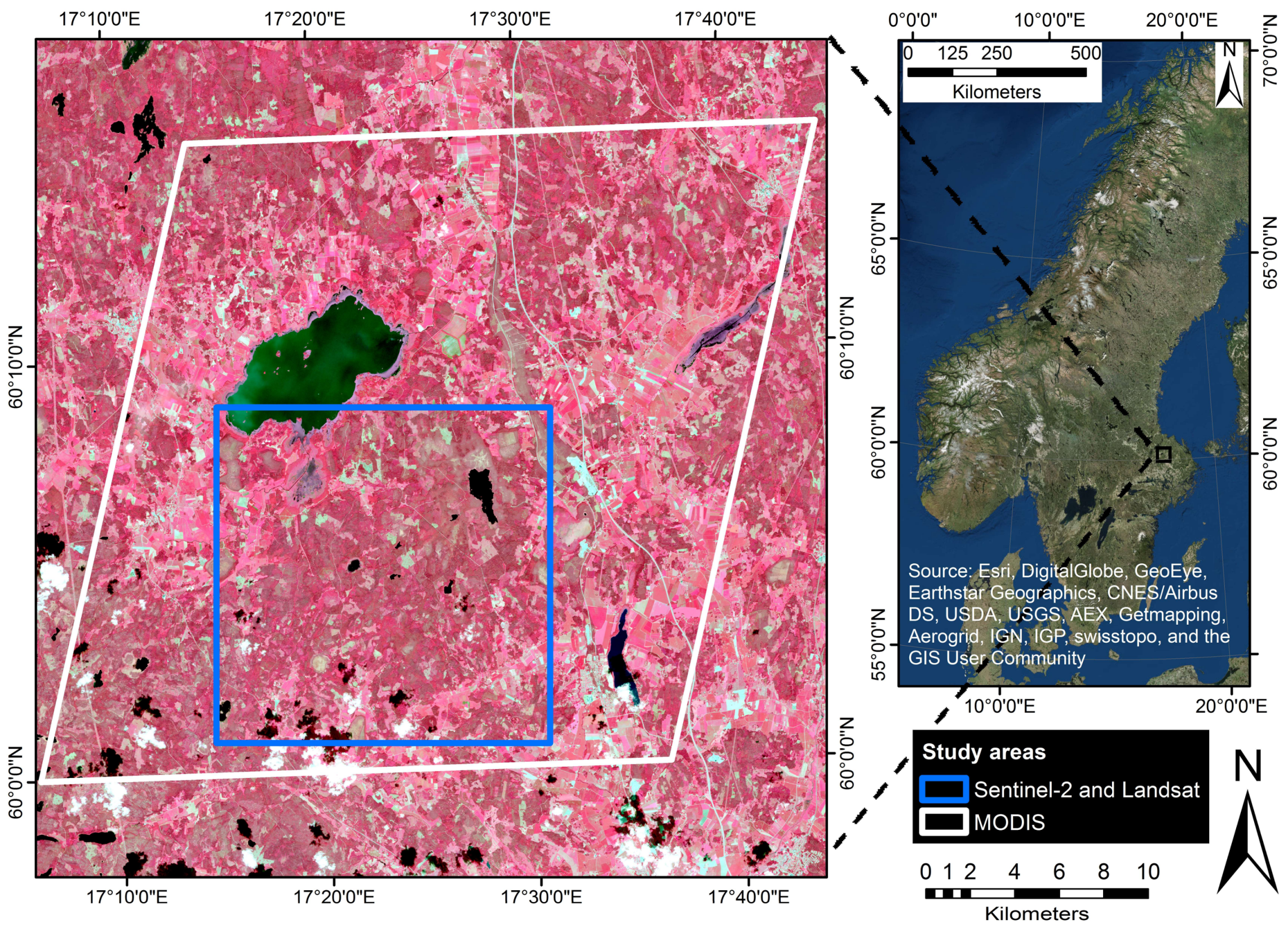
The study area, dominated by coniferous needle-leaf forest, mainly Scots pine (Pinus sylvestris) and Norwegian spruce (Picea abies), is located in central Sweden at around latitude 60°05′N, longitude 17°28′E (Figure 1). The area was specifically chosen to be challenging for seasonality modeling because it has weak annual NDVI amplitude, and is strongly influenced by winter darkness, snow dynamics, and clouds. In addition, it is located in a region where the number of Landsat observations is relatively low [1].
We used four remotely sensed data sets for developing and testing our processing method (Table 1): (1) Normalized Difference Vegetation Index (NDVI) time series generated from Landsat 5 and 7 sensors [1]. These data were pre-processed using FMASK (Function of Mask) [21] to generate quality assessment (QA) data (clear, water, cloud, cloud shadow and low quality for other reasons); (2) S2 data, pre-processed into level 2A top-of-canopy reflectance values using Sen2Cor [22]. The data were categorized into 11 classes by Sen2Cor, of which we regarded “vegetation” and “bare soils” as belonging to the clear-sky quality class; (3) Landsat 8 OLI NBAR 30m data from the Harmonized Landsat Sentinel-2 (HLS) surface reflectance product, which consists of Landsat and S2 observations, processed to have compatible radiometry and geometry [23]. The data include quality flags with labels identifying clouds, cirrus clouds, adjacent cloud, cloud shadow, snow or ice, water, and aerosol quality. All Landsat 8 scenes recorded at solar zenith angles >75° were labelled as low quality (non-clear) to exclude some unrealistically high NDVI values during winter that we observed in the product; (4) daily NDVI time series generated from the MODIS MOD09GA 500 m spatial resolution daily land surface reflectance dataset [24]. We used the 1 km Data State QA descriptors to exclude areas flagged as cloudy, cloud shadow, water bodies, aerosol-, cirrus-, fire-, or snow-contaminated.
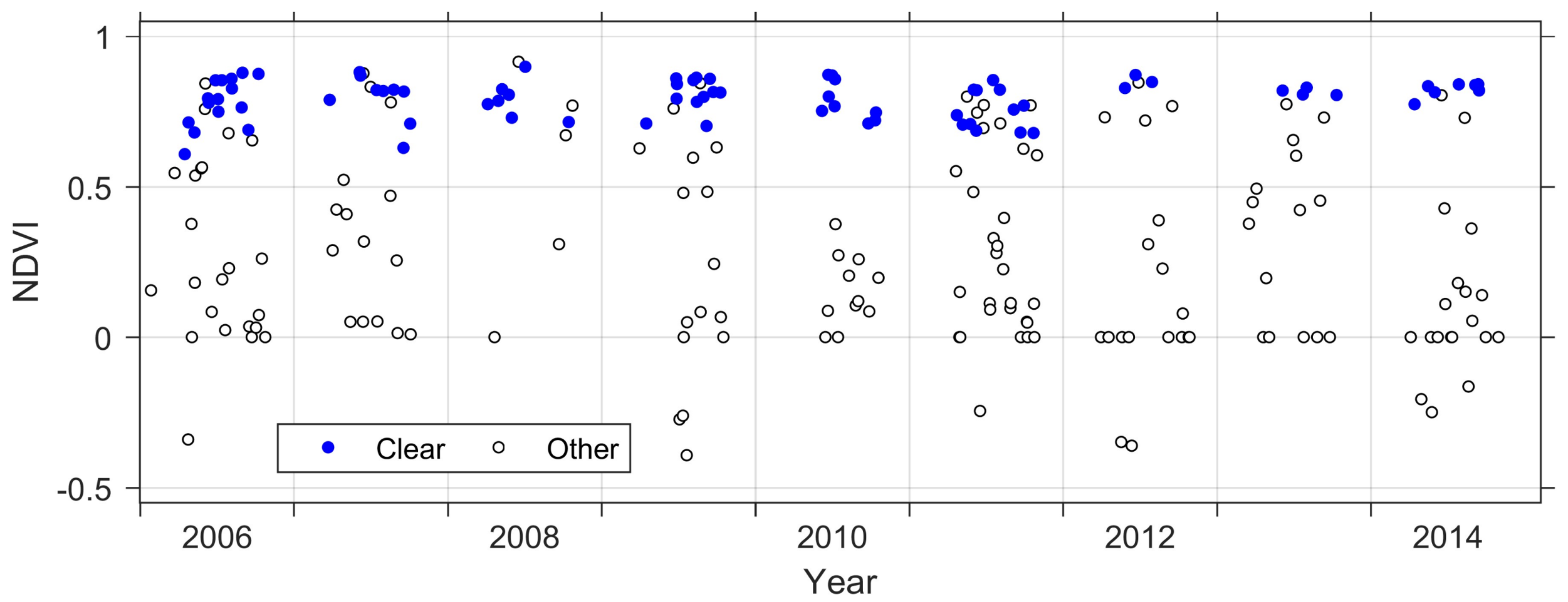
Landsat data extracted over the test area frequently show a large proportion of poor-quality observations (Figure 2). The time series in the example shows very weak seasonal dynamics, and estimating seasonality parameters from such data requires a very robust fitting method. Furthermore, the method should generate an output quality indicator that indicates if the data frequency is sufficient for generating reliable seasonal functions and parameters.
2.2. Assumptions and Modelling Principles
For simplicity, we assume that pixels that have undergone rapid transformation, i.e., due to clear cutting or fire, have been identified and excluded (e.g., using the Continuous Change Detection and Classification (CCDC) algorithm [21]). We also assume that variation in vegetation properties, and thus NDVI, is basically periodic, i.e., with one or more well-defined seasons per year. From these general principles, we desire a seasonal model that provides proper separation between clear and non-clear observations (cf. [11]), that is faithful to available data, and that considers the distribution bias inherent to vegetation index data due to e.g., undetected cloud contamination [25]. Our approach is based on the assumption that when data are scarce or lacking, an optimal fitting method should fall back on a seasonal shape prior, which we define here as a pre-computed time-profile that captures the average or climatological seasonal shape. This shape prior is especially useful when imputing values during periods of missing data, i.e. when linear interpolation, for example, might lead to erroneous results. The idea of lending stability from a pixel-based climatology has previously been shown to be useful [26]. A final principle underlying our approach is that statistics characterizing the quality of successful fits should be generated. Below we discuss the implementation of these modelling principles based on box constrained separable least squares fits to double logistic functions, combined with seasonal shape priors.
2.3. Implementation
2.3.1. Model Function and Shape Priors
The model function is a sum over basis functions, one for each season
As basis functions we take double logistic function [27]
although other functions, such as asymmetric Gaussians [28], are also possible. In Equation (1) the parameter determines the base level, and the linear parameters define the amplitudes for the seasons. The non-linear parameters and determine the left and right inflexion points for season , whereas and determine the time period of increase and decrease (hereafter, rise and fall time) respectively. The model function depends on the base level, linear parameters and non-linear parameters, and is flexible enough to encompass interannual seasonal shifts and variations. Under the assumption that all seasons have the same amplitude, the same rise time, the same fall time, and inflexion points shifted by multiples of 365 days, i.e., and , where , the model function gives an average description of data for all seasons. With the parameters fixed, as described above, we can interpret as a shape prior for season .
2.3.2. Base Level
Data acquired during the dormant (i.e., winter at northern latitudes) period define the level from which the NDVI values increase during the growing season. This base level depends on the snow-free reflectance of the soil background or perennial ground vegetation cover. If pixels that have undergone rapid transformations have been excluded, as discussed above, the base level should be constant or slowly varying. The base level could be established from field measurements or from satellite observations acquired directly prior to or after the growing period (to avoid snow, if present) [29,30]. However, in boreal forests, for example, these time periods are often characterized by cloudy conditions, and relatively few clear Landsat and S2 observations are generally available. To ensure sufficient data sampling of low-value vegetation observations, we suggest using a low percentile of the clear observation histogram for the complete time period, e.g., 5%. To generate more stable statistics, histograms can be generated from all observations in a spatial neighborhood of pixels with the same land cover class. To allow for gradual changes in base level, arising e.g., due to changes in understory vegetation cover, histograms could also be estimated from shorter periods where sufficient data are available.
2.3.3. Determining the Shape Prior
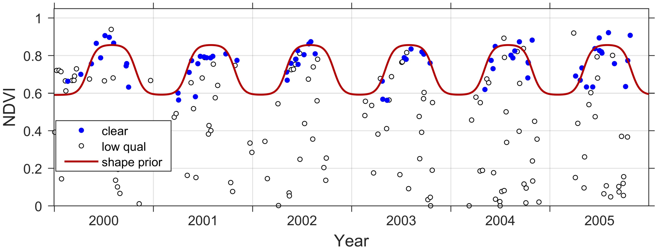
Once the base level has been established, the remaining five parameters—the common amplitude, the common rise time, the common fall time, and the shifted inflexion points—are determined, using an iterative upper envelope adapted separable least squares fit requiring a minimum of five high-quality data values [28,31]. In practice, to establish the shape prior firmly, more values are needed; the exact number depends on the distribut ion of the values in time. If desired, the procedure can be generalized and the parameters determined from all observations in a spatial neighborhood using pixels of the same land cover. The obtained function, as illustrated in Figure 3, gives a stable average global description of all data with a good separation between clear and non-clear observations. However, note that the shape prior function is not meant for describing intra-seasonal variations in NDVI.
2.3.4. Determining a Model Function That Accounts for Intra-Seasonal Variations
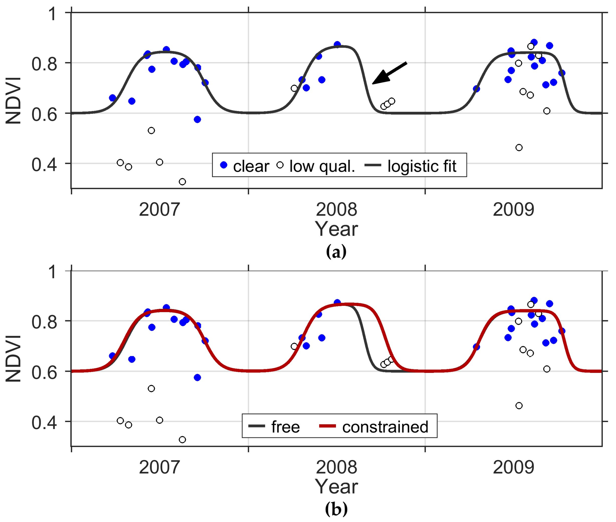
Similar to the shape prior, we define a model function that accounts for intra-seasonal variation and that is determined using an iterative upper envelope adapted separable least squares fit. For this case, however, each season has its own set of parameters that is independent of the parameters from the other seasons. The fitting accuracy depends on the number of high-quality data values and their distribution in time. When insufficient high-quality data are available during the beginning and end of the growing season, the resulting function fits can be unrealistic (Figure 4a). In these cases, one or more free seasonal parameters are assigned the values of the corresponding parameters of the shape prior, the effect of which is illustrated in Figure 4b.
Please note that although the parameters are allowed to vary independently from each other to account for intra-seasonal variations, there is, due to the global nature of the fit, an interaction between them. The resulting model function is not identical to the one obtained by doing a sequence of separate fits to the different years and merging the individual fits to a model for all years. The model function from a global fit, whether or not it falls back on shape priors, is always continuous and smooth, whereas the function obtained by merging functions from a number of individual fits is, in general, discontinuous. The degree of discontinuity in the latter depends on the shape of the underlying NDVI curve as well as on the quality of the data.
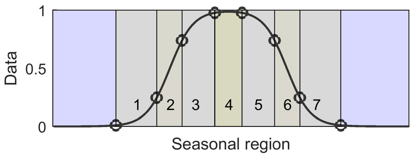
To determine the feasibility of using free parameters, here we propose evaluating the point distribution in time using seven regions of the seasonal curve (Figure 5). If no high-quality data points are found in the specified regions, according to Table 2, the free parameter is replaced by the corresponding parameter of the shape prior. This important feature prevents unrealistic fits during periods with sparse data.
Poor fitting leading to unrealistic seasons could also be caused by high levels of undetected noise in the data. Such periods are identified and handled by applying box constraints [32], in which the seasonal parameters (the amplitude, inflexion points, and the parameters determining the rise and fall time) are constrained within given intervals. This way, the fitted function can be prevented from varying more than a certain distance away from the shape prior, e.g., preventing the estimated spring or autumn dates from occurring more than a month before or after normal. The constraints are knowledge-based and class-specific, and hence must be prescribed (see Section 4). The described methods stabilize the fitting procedure, and have the added advantage that the shape prior can be used for gap filling over extended periods of missing data.
The use of shape prior parameters, rather than free parameters, can be recorded for each season, and each such occurrence recorded as a quality indicator. The indicators for a season can then be propagated to the seasonality parameters. Thus, for example, the start of season and length of season would only be assigned the highest quality if was computed with free parameters. Summing up the seasonal quality indicators for a dataset provides a measure of the general product quality and indicates its usefulness for seasonality estimation.
2.3.5. Data Storage and Compression
An added benefit of the model we describe is that it allows for a high degree of data compression. Storing the shape prior requires six parameters, and storing the full model function requires five parameters per season, plus the base level. Compared to storing daily data values and estimated seasonality parameters, the proposed method only uses a small fraction of the storage required for the full data set, depending on the chosen output time step. Using the estimated parameters, the model function can be projected on any desired time grid, and seasonality parameters, such as the start and end of growing seasons, can easily be computed.
2.3.6. Evaluating the Robustness of the Method
We evaluated the robustness of the fitting method, rather than analyzing its ability to estimate actual ground-observed phenology. The latter is a function of several factors of which the mathematical fitting method is only one. (It also depends on the remotely sensed data, the preprocessing methodology, criteria for defining phenological parameters, and vegetation type). We hence focused our analysis on a critical function for ensuring robustness: the use of shape prior. This is a key feature of the method that strongly affects the fitted curves.
To test this we used the MODIS 500 m daily dataset for the period 2011–2016, and extracted a 30.5 km × 30.5 km (61 × 61 pixels) region overlapping the test area (Figure 1). We then generated two datasets: one reference dataset based on all clear-sky daily MODIS observations, to which we fitted double-logistic functions and extracted dates of start-of-season (SOS) and end-of-season (EOS); and another dataset that was a sparse subset of the first one, simulating S2 by only including the clear-sky MODIS observations that correspond exactly in time with the observations from S2. For 2011–2015, i.e., prior to S2, we selected the same number of MODIS observations per year as in 2016. We then fitted double logistic functions to 2016 with and without 2011–2015 shape prior data, and compared SOS and EOS parameters with those estimated from the daily MODIS data.
Dates of SOS and EOS can be defined in many different ways, e.g., the time when the model function reaches prescribed fractions of the seasonal amplitude above the base level (e.g., 10%) [17,18]. The exact choice of definitions is not relevant to the model development described in this paper; we simply defined them based on the inflexion points of the fitted functions [5].
3. Results
The proposed processing method was successfully applied to Landsat and S2 data over the test area. Time series plots for three selected pixels are shown in Figure 6. These plots serve to demonstrate the seasonal fits and the effects of the difference in temporal sampling between Landsat and S2 for representative deciduous, coniferous, and agricultural pixels.
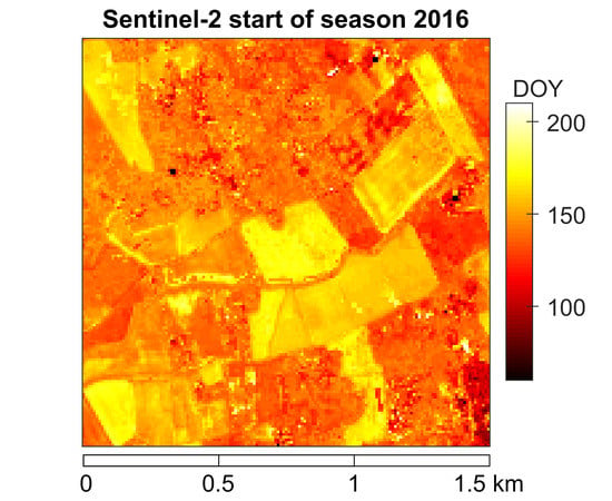
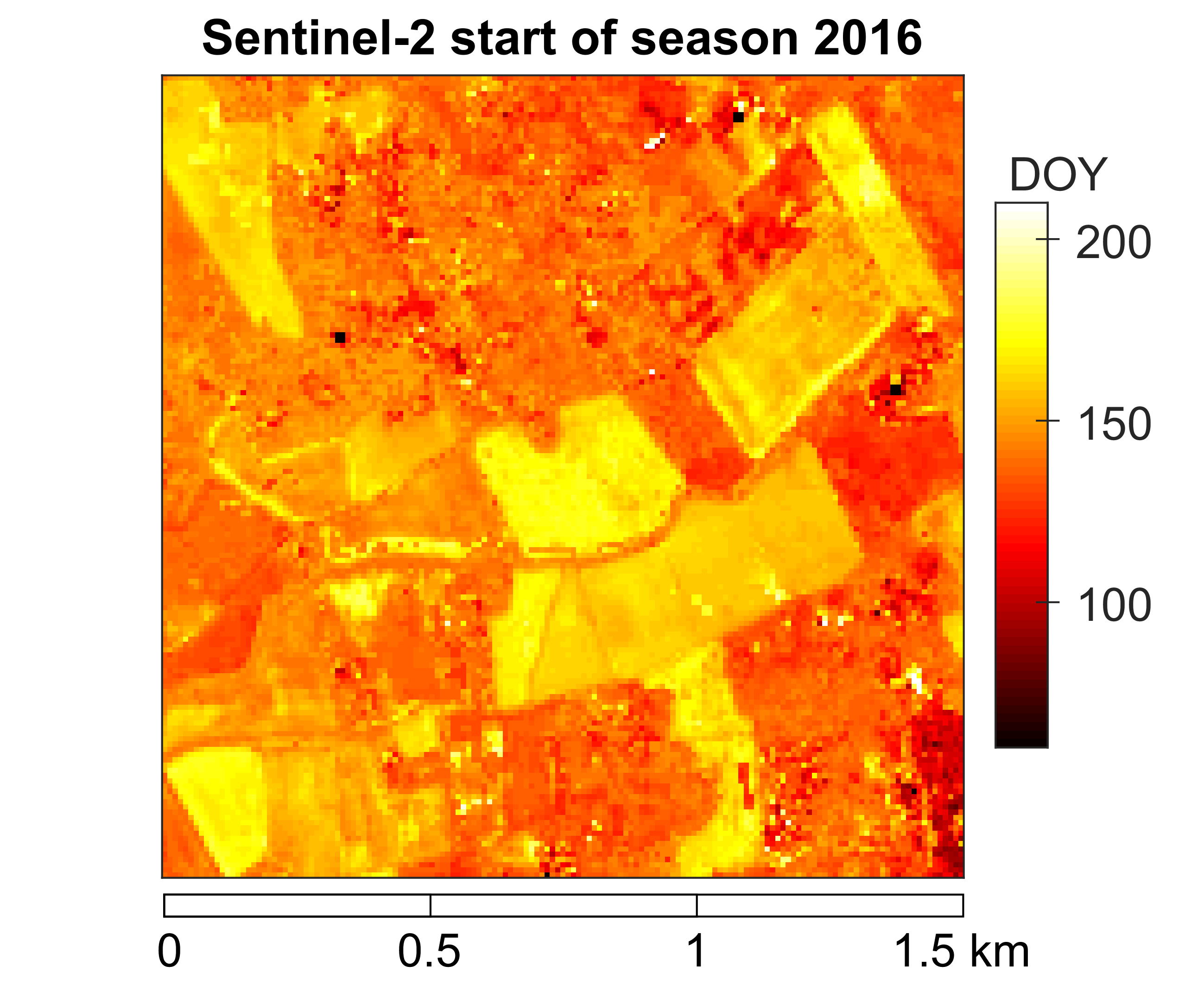
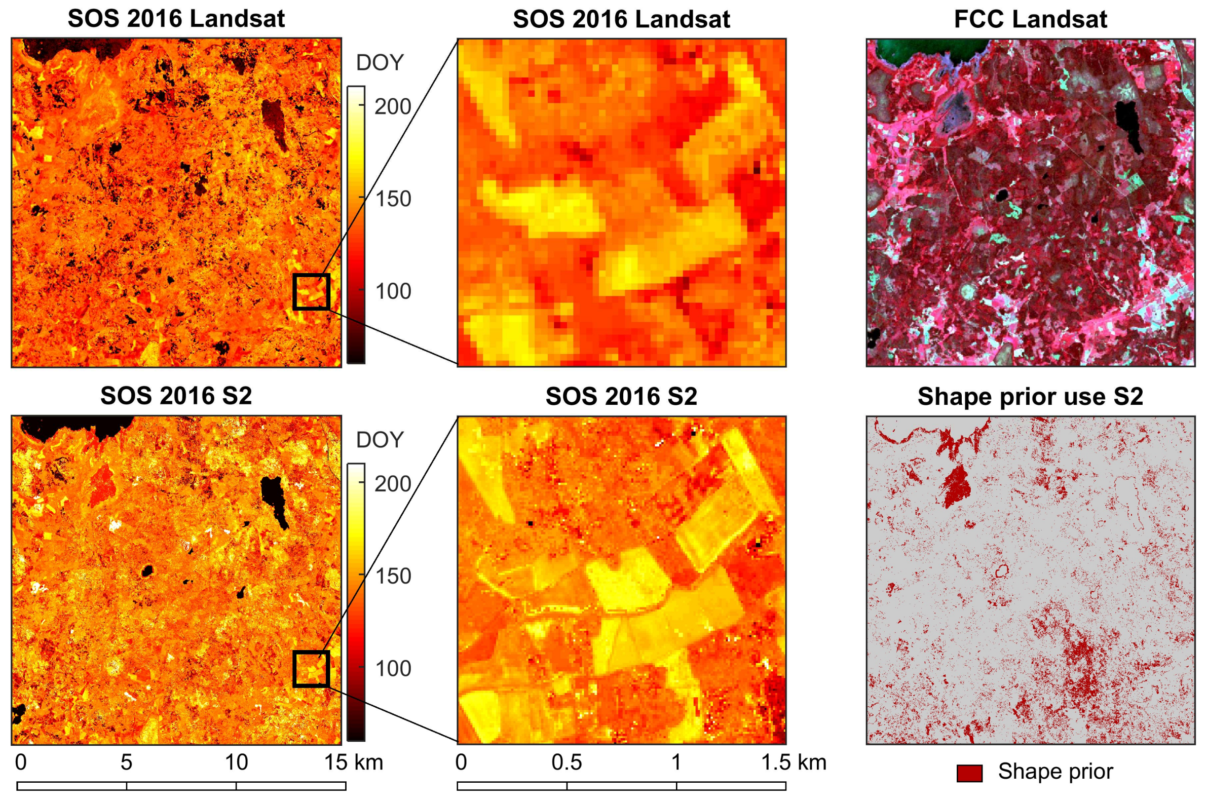
Maps were generated over the test area to show phenological parameters estimated from fitted functions for Landsat and S2a, e.g., the start of season date for 2016 (Figure 7). A false color composite (FCC) from Landsat is provided for comparison, along with a map that identifies pixels where the shape prior was used for estimating the parameter (12.2% of pixels). The basic landscape features are captured in the SOS maps estimated from both Landsat and S2, and the zoomed-in maps clearly show the greater phenological detail available from S2 compared to Landsat.
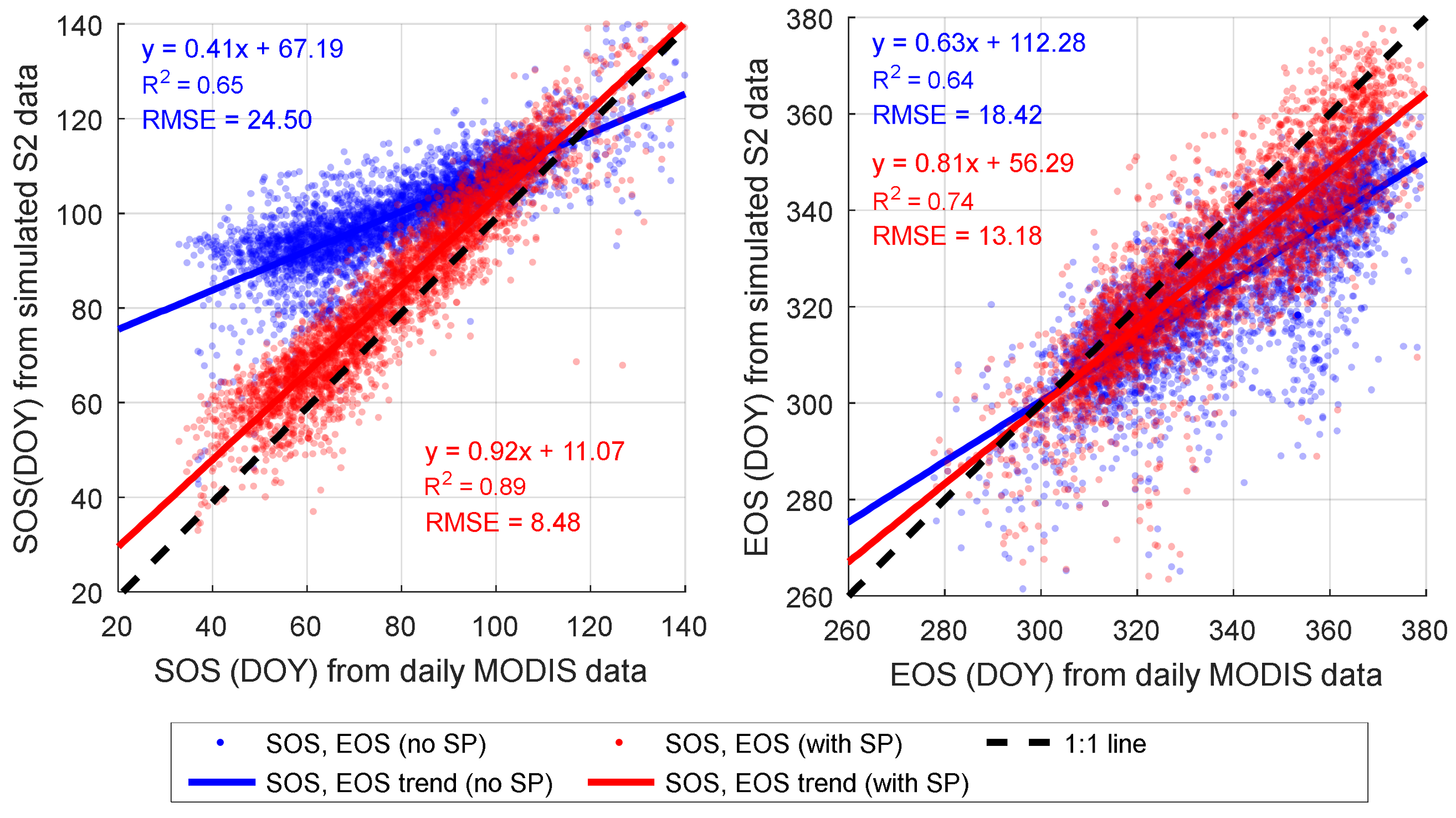
The significance of using the shape prior for estimates of SOS and EOS is shown in Figure 8. The left hand plot shows the bias when estimating SOS in 2016 from simulated S2 based on MODIS NDVI without shape prior (blue symbols), compared to the inclusion of shape prior data from 2011–2015 (red symbols). The shape prior estimates align well with the estimates from the daily MODIS data (Root Mean Squared Error, RMSE = 8.5 days), whereas the estimates without shape prior have a large RMSE of 24.5 days. For EOS in the right hand plot the difference is smaller; the RMSE is reduced from 18.4 days to 13.2 days, however, again with a clearly visible bias away from the 1:1 line when the shape prior data are not used.
4. Discussion
The combination of the shape prior and box constrained least squares fits provide stability to the estimates, and reduce the risk of poor fitting due to sparse data. Pixel quality information can be used as weights in the function fitting, or as in our case, to exclude low-quality observations. In Figure 6 and Figure 7 the shape prior for S2 was based on a short time series from 2015 through to June 2017; data from more years would have been needed to estimate the shape prior parameters accurately. Hence, for pixels in our test data where the shape prior was used, annual phenology estimates are probably not accurate. However, it should be noted that we only used one of the S2 satellites, since S2b was not operational in 2016, and we anticipate considerable improvement when data from both S2 satellites are included. An alternative to using time series data for determining the shape prior is to base it on a larger domain of data, i.e., by spatial sampling. It may also be possible to combine different satellite systems to achieve increased accuracy in the estimation. This, of course, requires that the two data sources are spatially and radiometrically harmonized, such as in the HLS dataset [23].
The base level can be defined by several methods: by evaluating historical time-series data at each pixel; by analyzing a large number of pixels from the same class in a spatial neighborhood; by using spectral ground measurements [33]; or by sampling data during parts of the off-seasonal period of the year (e.g., [30]). In a similar way, specifications of the constraints on the parameter values should be supplied. These could be based on statistics for a sufficient number of pixels, or based on heuristics developed from information about known phenological conditions (e.g., the maximum time that a growing season in a certain area is expected to vary). Today, global databases of phenology from coarse-resolution sensors exist that may be utilized for this purpose, e.g., the MODIS MCD12Q2 global land cover dynamics product (https://lpdaac.usgs.gov) [5]. For determining base level and constraints, it is necessary to identify and avoid pixels with rapid land cover variations, i.e., by using the method by Zhu et al. [11].
There is no consensus in the remote sensing literature as to the superiority of any particular fitting method over others, and different methods have been found to be optimal under different conditions (cf. comparisons in [4,34,35,36,37]). However, we argue that the choice of fitting method ultimately depends on the frequency, distribution, and quality of the input data. Where the data quality is sufficiently high for choosing methods that preserve intra-seasonal variations, like smoothing filters (e.g., Savitzky-Golay [38]) or splines (e.g., the Whittaker smoother [39,40]), these methods should be chosen. However, in the case of lower frequencies of data, as with current Landsat and Sentinel-2 data over most areas, function fitting may be the only option for achieving robustness. Fits to double logistic functions are widely used for estimating phenology, and have been applied to both MODIS [5] and Landsat data [8]. These functions are well tested for estimating phenology [5,8,29,41], and were recently shown to be robust for phenological parameter estimation under a variety of conditions [34].
The logistic basis functions we use in this paper work well with data in many types of natural systems. In cases with more abrupt seasonal changes, e.g., agricultural lands, it may be preferable to use asymmetric Gaussian functions [28], which have the ability to capture rapid shifts with relatively few parameters. In agricultural regions with annually shifting seasonality, it may also be necessary to establish the shape prior from different pixels from the same field or crop, rather than from time-series from the same field.
It may also be useful to add parameters that allow for more flexible representations of seasonality, for example, to better model the green-down period after the seasonal maximum [13]. However, since we model each year individually rather than pooling all data as in these studies, we have fewer data points each year; this may cause overfitting or lack of stability. Hence, the use of more complex fitting procedures probably requires evaluation using metrics such as the Akaike information criterion [42]. Our method has several advantages compared to other methods based on only logistic or similar functions: it handles all seasons simultaneously, yielding a smooth model and avoiding unrealistic basis level discontinuities between the seasons; it provides quality indicators associated with values estimated for model parameters; and it is numerically stable due to its formulation in terms of separable least squares. The method is also flexible in the sense that it can work with or without a shape prior depending on data frequency and quality, and no prior interpolation of data is necessary. Furthermore, our method can be useful for generating fitting parameters when warping data from one sensor or year onto another [43].
Further tests will have to be made in different environments and with different data types to fine-tune the method. In addition, it may be necessary to define certain land-cover specific tolerances with respect to the allowed growing season variation: A boreal evergreen forest is not expected to vary with respect to seasonality events by more than a few weeks, whereas an agricultural field can vary quite freely depending on agricultural practices. Further development to adapt to different monitoring conditions and geographical areas will be necessary to enable operational implementation of the method.
For full understanding of the accuracy of the method, and phenology estimation from medium resolution data in general, it will be necessary to analyze obtained parameters against field measurements of phenology, e.g., from phenological cameras [44], flux towers [45], or field spectral measurements [33].
5. Conclusions
With the proposed method, which is based on a box constrained separable least squares fitting to logistic model functions, we have developed a flexible and robust method for modeling the phenology of growing seasons with data from medium-resolution optical satellites like Landsat and Sentinel-2. We show that the use of the shape prior adds robustness to the function fitting. The method relies on accurate labeling of pixel quality, and, in order to obtain stable parameters, on the availability of data from long time series (or alternatively from a larger spatial domain). For Sentinel-2, this means that extending the time series backwards using the Landsat record may be required during the first years of operation. We also conclude that further testing will be necessary in different biomes to understand better how to choose parameters for base level and parameter constraints. The proposed method is implemented in the TIMESAT software package [17] and will be available in future releases.
Acknowledgments
This work was financed by the Swedish National Space board under a grant to Lars Eklundh and Per Jönsson, Dnr. 119/13. Work by co-authors at Boston University was partly supported by NASA Grant number NNX15AK60G. We acknowledge the NASA Land Processes Distributed Active Archive Center (LP DAAC), USGS/Earth Resources Observation and Science (EROS) Center, Sioux Falls, South Dakota for providing data from MODIS and Landsat sensors. We thank Damien Sulla-Menashe, Boston University, for access to processed Landsat data. For access to S2 data we acknowledge the European Commission and the Copernicus Open Access Hub, and for access to HLS data we acknowledge the NASA HLS team under Jeffrey Masek.
Author Contributions
P.J. developed the mathematical model with input from L.E. and Z.C., P.J. and Z.C. wrote the software; Z.C. implemented the method and performed all data analyses; E.M. and M.A.F. contributed with Landsat data, advice, and editing of the paper; and L.E. authored the paper with significant input from all authors.
Conflicts of Interest
The authors declare no conflict of interest.
References
- Wulder, M.A.; White, J.C.; Loveland, T.R.; Woodcock, C.E.; Belward, A.S.; Cohen, W.B.; Fosnight, E.A.; Shaw, J.; Masek, J.G.; Roy, D.P. The global Landsat archive: Status, consolidation, and direction. Remote Sens. Environ. 2016, 185, 271–2283. [Google Scholar] [CrossRef]
- Justice, C.O.; Townshend, J.R.G.; Holben, B.N.; Tucker, C.J. Analysis of the phenology of global vegetation using meteorological satellite data. Int. J. Remote Sens. 1985, 6, 1271–1318. [Google Scholar] [CrossRef]
- Wang, Y.; Zhao, J.; Zhou, Y.; Zhang, H. Variation and trends of landscape dynamics, land surface phenology and net primary production of the Appalachian Mountains. J. Appl. Remote Sens. 2012, 6, 061708. [Google Scholar] [CrossRef]
- White, M.A.; De Beurs, K.M.; Didan, K.; Inouye, D.W.; Richardson, A.D.; Jensen, O.P.; O’Keefe, J.; Zhang, G.; Nemani, R.R.; Van Leeuwen, W.J.D.; et al. Intercomparison, interpretation, and assessment of spring phenology in North America estimated from remote sensing for 1982–2006. Glob. Chang. Biol. 2009, 15, 2335–2359. [Google Scholar] [CrossRef]
- Zhang, X.; Friedl, M.A.; Schaaf, C.B.; Strahler, A.H.; Hodges, J.C.F.; Gao, F.; Reed, B.C.; Huete, A. Monitoring vegetation phenology using MODIS. Remote Sens. Environ. 2003, 84, 471–475. [Google Scholar] [CrossRef]
- Jin, H.X.; Jönsson, A.M.; Bolmgren, K.; Langvall, O.; Eklundh, L. Disentangling remotely-sensed plant phenology and snow seasonality at northern Europe using MODIS and the plant phenology index. Remote Sens. Environ. 2017, 198, 203–212. [Google Scholar] [CrossRef]
- Fisher, J.I.; Mustard, J.F.; Vadeboncoeur, M.A. Green leaf phenology at Landsat resolution: Scaling from the field to the satellite. Remote Sens. Environ. 2006, 100, 265–279. [Google Scholar] [CrossRef]
- Melaas, E.K.; Friedl, M.A.; Zhu, Z. Detecting interannual variation in deciduous broadleaf forest phenology using Landsat TM/ETM+ data. Remote Sens. Environ. 2013, 132, 176–185. [Google Scholar] [CrossRef]
- Wulder, M.A.; White, J.C.; Coops, N.C.; Butson, C.R. Multi-temporal analysis of high spatial resolution imagery for disturbance monitoring. Remote Sens. Environ. 2008, 112, 2729–2740. [Google Scholar] [CrossRef]
- Kennedy, R.E.; Yang, Z.; Cohen, W.B. Detecting trends in forest disturbance and recovery using yearly Landsat time series: 1. LandTrendr—Temporal segmentation algorithms. Remote Sens. Environ. 2010, 114, 2897–2910. [Google Scholar] [CrossRef]
- Zhu, Z.; Woodcock, C.E.; Olofsson, P. Continuous monitoring of forest disturbance using all available Landsat imagery. Remote Sens. Environ. 2012, 122, 75–91. [Google Scholar] [CrossRef]
- Fisher, J.I.; Mustard, J.F. Cross-scalar satellite phenology from ground, Landsat, and MODIS data. Remote Sens. Environ. 2007, 109, 261–273. [Google Scholar] [CrossRef]
- Elmore, A.J.; Guinn, S.M.; Minsley, B.J.; Richardson, A.D. Landscape controls on the timing of spring, autumn, and growing season length in mid-Atlantic forests. Glob. Chang. Biol. 2012, 18, 656–674. [Google Scholar] [CrossRef]
- Melaas, E.K.; Sulla-Menashe, D.; Gray, J.M.; Black, T.A.; Morin, T.H.; Richardson, A.D.; Friedl, M.A. Multisite analysis of land surface phenology in North American temperate and boreal deciduous forests from Landsat. Remote Sens. Environ. 2016, 186, 452–464. [Google Scholar] [CrossRef]
- Friedl, M.A.; Gray, J.M.; Melaas, E.K.; Richardson, A.D.; Hufkens, K.; Keenan, T.F.; Bailey, A.; O’Keefe, J. A tale of two springs: Using recent climate anomalies to characterize the sensitivity of temperate forest phenology to climate change. Environ. Res. Lett. 2014, 9, 054006. [Google Scholar] [CrossRef]
- Melaas, E.K.; Sulla-Menashe, D.; Friedl, M.A. Multidecadal changes and interannual variation in springtime phenology of North American temperate and boreal deciduous forests. Geophys. Res. Lett. 2018, 45. [Google Scholar] [CrossRef]
- Jönsson, P.; Eklundh, L. TIMESAT—A program for analysing time-series of satellite sensor data. Comput. Geosci. 2004, 30, 833–845. [Google Scholar] [CrossRef]
- Eklundh, L.; Jönsson, P. TIMESAT 3.3 with Seasonal Trend Decomposition and Parallel Processing Software Manual; Lund University: Lund, Sweden, 2017; p. 88. [Google Scholar]
- Roerink, G.J.; Menenti, M.; Verhoef, W. Reconstructing cloudfree NDVI composites using Fourier analysis of time series. Int. J. Remote Sens. 2000, 21, 1911–1917. [Google Scholar] [CrossRef]
- Ivits, E.; Cherlet, M.; Mehl, W.; Sommer, S. Ecosystem functional units characterized by satellite observed phenology and productivity gradients: A case study for Europe. Ecol. Indic. 2013, 27, 17–28. [Google Scholar] [CrossRef]
- Zhu, Z.; Woodcock, C.E. Automated cloud, cloud shadow, and snow detection in multitemporal Landsat data: An algorithm designed specifically for monitoring land cover change. Remote Sens. Environ. 2014, 152, 217–234. [Google Scholar] [CrossRef]
- Muller-Wilm, U.; Louis, J.; Richter, R.; Gascon, F.; Niezette, M. Sentinel-2 level 2A prototype processor: Architecture, algorithms and first results. In Proceedings of the 2013 ESA Living Planet Symposium, Edinburgh, UK, 9–13 September 2013; pp. 9–13. [Google Scholar]
- Claverie, M.; Masek, J.G.; Ju, J. Harmonized Landsat-8 Sentinel-2 (HLS) Product User’s Guide. 2017. Available online: https://hls.gsfc.nasa.gov (accessed on 15 February 2018).
- Vermote, E.; Wolfe, R. MOD09GA MODIS/Terra Surface Reflectance Daily L2G Global 1 km and 500 m SIN Grid V006. 2015. Available online: https://doi.org/10.5067/MODIS/MOD09GA.006 (accessed on 9 January 2018).
- Holben, B.N. Characteristics of maximum-value composite images from temporal AVHRR data. Int. J. Remote Sens. 1986, 7, 1417–1443. [Google Scholar] [CrossRef]
- Klisch, A.; Atzberger, C. Operational Drought Monitoring in Kenya Using MODIS NDVI Time Series. Remote Sens. 2016, 8, 267. [Google Scholar] [CrossRef]
- Fischer, A. A model for the seasonal variations of vegetation indices in coarse resolution data and its inversion to extract crop parameters. Remote Sens. Environ. 1994, 48, 220–230. [Google Scholar] [CrossRef]
- Jönsson, P.; Eklundh, L. Seasonality extraction by function fitting to time-series of satellite sensor data. IEEE Trans. Geosci. Remote Sens. 2002, 40, 1824–1832. [Google Scholar] [CrossRef]
- Beck, P.S.A.; Atzberger, C.; Hogda, K.A.; Johansen, B.; Skidmore, A.K. Improved monitoring of vegetation dynamics at very high latitudes: A new method using MODIS NDVI. Remote Sens. Environ. 2006, 100, 321–334. [Google Scholar] [CrossRef]
- Beck, P.S.A.; Jönsson, P.; Hogda, K.A.; Karlsen, S.R.; Eklundh, L.; Skidmore, A.K. A ground-validated NDVI dataset for monitoring vegetation dynamics and mapping phenology in Fennoscandia and the Kola peninsula. Int. J. Remote Sens. 2007, 28, 4311–4330. [Google Scholar] [CrossRef]
- Nielsen, H.B. Separable Nonlinear Least Squares, Technical Report IMM-REP-2000-01, Informatics and Mathematical Modeling (IMM); Technical University of Denmark: Lyngby, Denmark, 2000. [Google Scholar]
- Coleman, T.F.; Li, Y. An Interior, Trust Region Approach for Nonlinear Minimization Subject to Bounds. SIAM J. Optim. 1996, 6, 418–455. [Google Scholar] [CrossRef]
- Eklundh, L.; Jin, H.X.; Schubert, P.; Guzinski, R.; Heliasz, M. An Optical Sensor Network for Vegetation Phenology Monitoring and Satellite Data Calibration. Sensors 2011, 11, 7678–7709. [Google Scholar] [CrossRef] [PubMed]
- Cai, Z.Z.; Jönsson, P.; Jin, H.X.; Eklundh, L. Performance of Smoothing Methods for Reconstructing NDVI Time-Series and Estimating Vegetation Phenology from MODIS Data. Remote Sens. 2017, 9, 1271. [Google Scholar] [CrossRef]
- Hird, J.N.; McDermid, G.J. Noise reduction of NDVI time series: An empirical comparison of selected techniques. Remote Sens. Environ. 2009, 113, 248–258. [Google Scholar] [CrossRef]
- Atkinson, P.M.; Jeganathan, C.; Dash, J.; Atzberger, C. Inter-comparison of four models for smoothing satellite sensor time-series data to estimate vegetation phenology. Remote Sens. Environ. 2012, 123, 400–417. [Google Scholar] [CrossRef]
- Geng, L.; Ma, M.; Wang, X.; Yu, W.; Jia, S.; Wang, H. Comparison of Eight Techniques for Reconstructing Multi-Satellite Sensor Time-Series NDVI Data Sets in the Heihe River Basin, China. Remote Sens. 2014, 6, 2024. [Google Scholar] [CrossRef]
- Chen, J.; Jönsson, P.; Tamura, M.; Gu, Z.H.; Matsushita, B.; Eklundh, L. A simple method for reconstructing a high-quality NDVI time-series data set based on the Savitzky-Golay filter. Remote Sens. Environ. 2004, 91, 332–344. [Google Scholar] [CrossRef]
- Atzberger, C.; Eilers, P.H.C. A time series for monitoring vegetation activity and phenology at 10-daily time steps covering large parts of South America. Int. J. Digit. Earth 2011, 4, 365–386. [Google Scholar] [CrossRef]
- Eilers, P.H.C. A Perfect Smoother. Anal. Chem. 2003, 75, 3631–3636. [Google Scholar] [CrossRef] [PubMed]
- Fisher, A. A simple model for the temporal variations of NDVI at regional scale over agricultural countries. Validations with ground radiometric measurements. Int. J. Remote Sens. 1994, 15, 1421–1446. [Google Scholar] [CrossRef]
- Akaike, H. Likelihood of a model and information criteria. J. Econom. 1981, 16, 3–14. [Google Scholar] [CrossRef]
- Baumann, M.; Ozdogan, M.; Richardson, A.D.; Radeloff, V.C. Phenology from Landsat when data is scarce: Using MODIS and Dynamic Time-Warping to combine multi-year Landsat imagery to derive annual phenology curves. Int. J. Appl. Earth Obs. 2017, 54, 72–83. [Google Scholar] [CrossRef]
- Richardson, A.D.; Jenkins, J.P.; Braswell, B.H.; Hollinger, D.Y.; Ollinger, S.V.; Smith, M.-L. Use of digital webcam images to track spring green-up in a deciduous broadleaf forest. Oecologia 2007, 152, 323–334. [Google Scholar] [CrossRef] [PubMed]
- Melaas, E.K.; Richardson, A.D.; Friedl, M.A.; Dragoni, D.; Gough, C.M.; Herbst, M.; Montagnani, L.; Moors, E. Using FLUXNET data to improve models of springtime vegetation activity onset in forest ecosystems. Agric. For. Meteorol. 2013, 171, 46–56. [Google Scholar] [CrossRef]
Figure 1.
Study area in Central Sweden. The image to the left is a false color composite from Sentinel-2, acquired on 8 July 2016. The white line marks the area of the MODIS data used, and the blue line marks the area of the Sentinel-2 and Landsat data used.
Figure 1.
Study area in Central Sweden. The image to the left is a false color composite from Sentinel-2, acquired on 8 July 2016. The white line marks the area of the MODIS data used, and the blue line marks the area of the Sentinel-2 and Landsat data used.

Figure 2.
Landsat observations for 2006–2014 extracted for a pine forest pixel (60.0863°N, 17.4795°E) denoted as “Clear” or “Other” (i.e., assigned another QA class than clear-sky in the FMASK algorithm). Note the large proportion of non-clear observations and the weak seasonal dynamics for this pixel.

Figure 3.
Shape prior for time series data from Landsat NDVI 2000–2005. The base level has, after analyzing the histogram for this pixel, been fixed to NDVI = 0.59. As the shape prior does not describe individual years, its main use is for stabilizing the fitting procedure during data-sparse periods.

Figure 4.
(a) Double logistic fits with free seasonal parameters. Note the unrealistically short second growing season due to lack of clear observations at the end of the season (arrow); (b) fit where the right inflexion point and the parameter determining the fall time are constrained and taken as the corresponding values of the shape prior.

Figure 5.
Seven regions in which data points must exist, according to Table 2, to allow free parameters to be used. Circles denote levels 0.01, 0.25, 0.75 and 0.99 of the amplitude to the left and right of the center.
Figure 5.
Seven regions in which data points must exist, according to Table 2, to allow free parameters to be used. Circles denote levels 0.01, 0.25, 0.75 and 0.99 of the amplitude to the left and right of the center.

Figure 6.
Examples of time series over deciduous (top), coniferous (middle), and agricultural (bottom) areas from Landsat (left) and S2 (right).
Figure 6.
Examples of time series over deciduous (top), coniferous (middle), and agricultural (bottom) areas from Landsat (left) and S2 (right).

Figure 7.
Phenology data from Landsat (top row) and Sentinel 2a (bottom row). Left hand images show estimated start of season (unit: day-of-year, DOY), and the center images show zoom-ins over an agricultural area. The right hand top image shows a false color composite (FCC) from Landsat 8 for comparison, and the bottom right image shows pixels where shape prior was used for estimating parameter , determining the start of season. Coordinates of the study area are shown in Figure 1.

Figure 8.
Reduced RMSE and bias when estimating start of season (left) and end of season (right) for 2016 from simulated S2 NDVI data by double logistic function fitting without shape prior (SP; blue dots) as compared to fitting with shape prior (red dots). Parameters from simulated S2 data are plotted against reference data of SOS and EOS from daily MODIS NDVI. Equations and statistics of the linear relationships are printed in the graph in blue (no SP) and red (with SP).


Table 1.
Data sources used in the study.
| No. | Source | Time Period | No. of Scenes/Tiles |
|---|---|---|---|
| 1 | Landsat 5 and 7 | January 2000–December 2014 | 452 |
| 2 | Landsat 8 (HLS) | March 2013–April 2017 | 352 |
| 3 | Sentinel-2 | July 2015–July 2017 | 109 |
| 4 | MODIS MOD09GA 500 m | January 2011–December 2016 | 2190 |
Table 2.
Parameters in Equations (1) and (2), and the corresponding regions in Figure 5, in which at least one point is required to allow the parameter to vary freely. If no points are found in a region, the corresponding parameter from the shape prior is used.
Table 2.
Parameters in Equations (1) and (2), and the corresponding regions in Figure 5, in which at least one point is required to allow the parameter to vary freely. If no points are found in a region, the corresponding parameter from the shape prior is used.
| Parameter | Seasonal Region (Figure 5) |
|---|---|
| 4 OR (2 AND 3 AND 5 AND 6) | |
| 2 OR (1 AND 3) | |
| 1 AND 3 | |
| 6 OR (5 AND 7) | |
| 5 AND 7 |
© 2018 by the authors. Licensee MDPI, Basel, Switzerland. This article is an open access article distributed under the terms and conditions of the Creative Commons Attribution (CC BY) license (http://creativecommons.org/licenses/by/4.0/).
Share and Cite
MDPI and ACS Style
Jönsson, P.; Cai, Z.; Melaas, E.; Friedl, M.A.; Eklundh, L. A Method for Robust Estimation of Vegetation Seasonality from Landsat and Sentinel-2 Time Series Data. Remote Sens. 2018, 10, 635. https://doi.org/10.3390/rs10040635
AMA Style
Jönsson P, Cai Z, Melaas E, Friedl MA, Eklundh L. A Method for Robust Estimation of Vegetation Seasonality from Landsat and Sentinel-2 Time Series Data. Remote Sensing. 2018; 10(4):635. https://doi.org/10.3390/rs10040635
Chicago/Turabian StyleJönsson, Per, Zhanzhang Cai, Eli Melaas, Mark A. Friedl, and Lars Eklundh. 2018. "A Method for Robust Estimation of Vegetation Seasonality from Landsat and Sentinel-2 Time Series Data" Remote Sensing 10, no. 4: 635. https://doi.org/10.3390/rs10040635
Note that from the first issue of 2016, this journal uses article numbers instead of page numbers. See further details here.