Soil Moisture and Vegetation Water Content Retrieval Using QuikSCAT Data


1
Jet Propulsion Laboratory, California Institute of Technology, 4800 Oak Grove Dr, Pasadena, CA 91109, USA
2
Naval Research Laboratory, 4555 Overlook Ave., SW, Washington, DC 20375, USA
*
Author to whom correspondence should be addressed.
Remote Sens. 2018, 10(4), 636; https://doi.org/10.3390/rs10040636
Submission received: 2 March 2018
/
Revised: 29 March 2018
/
Accepted: 12 April 2018
/
Published: 20 April 2018
Abstract
:Climate change and hydrological cycles can critically impact future water resources. Uncertainties in current climate models result in disagreement on the amount of water resources. Soil moisture and vegetation water content are key environmental variables on evaporation and transpiration at the land–atmosphere boundary. Radar remote sensing helps to improve our estimate of water resources spatially and temporally. This work proposes a backscattered power formulation for the Ku-band. Li et al. (2010) retrieved soil moisture and vegetation water content values using Windsat data and simultaneous collocated QuikSCAT backscattered power are used to estimate different parameters of backscatter formulation. These parameters are used to estimate soil moisture and vegetation water content using QuikSCAT power everywhere and every day during the summer season. The 2-folded cross validation method is used to evaluate the performance of soil moisture and vegetation water content retrieval. A relatively large correlation is observed between vegetation water content using WindSat and QuikSCAT data in land classes of Evergreen Needleleaf, Evergreen Broadleaf, Deciduous Broadleaf, and Mixed Forests. Similarly, the retrieved soil moisture using QuikSCAT in areas with bare surface fraction of greater than 60% shows relatively high correlation with WindSat values. QuikSCAT satellite collects data over land globally almost every day. Therefore, QuikSCAT data can be used to generate a global map of soil moisture and vegetation water content daily from 2000 to 2009.
1. Introduction
Vegetation water content and soil moisture are two key factors in climate and hydrological cycles. Because in situ soil moisture and vegetation water content measurements in particular are generally expensive and often problematic, no large-area soil moisture or vegetation water content products exist at fine spatial and temporal resolution. Radar remote sensing has been a successful tool to monitor these two parameters and their dynamics globally with high resolution.
Microwave measurements have the benefit of being largely unaffected by cloud cover and variable surface solar illumination. Passive microwave remote sensing of soil moisture has been performed extensively for more than three decades. Several multifrequency spaceborne microwave radiometers have significant sm (soil moisture) sensitivity in the 6–37 GHz frequency range. These include the Scanning Multichannel Microwave Radiometer (SMMR) launched in 1978, the Tropical Rainfall Measuring Mission (TRMM) Microwave Imager (TMI) in 1997, the Advanced Microwave Scanning Radiometer on board EOS Aqua (AMSR-E) in 2002, the WindSat radiometer in 2003, and Soil Moisture and Ocean Salinity (SMOS) L-band mission in 2009. Current L-band NASA mission SMAP (Soil Moisture Active Passive) measures the amount of water in the top 5 cm of soil everywhere on Earth’s surface. NASA’s future mission, SWOT (Surface Water Ocean Topography), is designed for monitoring water resources and their variations at Ka-band. The soil moisture retrieval algorithms for these missions try to separate the effects of soil moisture from vegetation water content. Therefore, different models are developed to extract both vegetation water content and soil moisture from these data sets [1,2,3]. The radar backscattering coefficient is used to model soil moisture and vegetation water content at different frequencies, especially at lower frequencies such as L-band and C-band. The use of L-band radar rather than higher frequencies such as C- and X-band is shown to be advantageous in reducing the effect of vegetation on measured cross sections from terrestrial surfaces [4,5]. Therefore, spaceborne missions such as SMOS, SMAP and Argentine Microwaves Observation Satellite (SAOCOM) are all dedicated for soil moisture monitoring at L-band. Different models for radar backscattering coefficients are developed for land surface at L-band [6,7,8,9].
QuikSCAT is originally designed to measure sea winds. However, the backscattered power of QuikSCAT can also be used over land. QuikSCAT Ku-band wave penetrates very little into the vegetation cover due to its large attenuation. Therefore, it can be used to study different effects in vegetated regions. The QuikSCAT data is used in densely forested areas like the Amazon to investigate the effect of drought [2]. Yang et al. [10] demonstrated a large correlation between QuikSCAT and Leaf Area Index (LAI). They also showed a linear relationship between VV/HH QuikSCAT backscatter and LAI for short and sparse vegetation but not for densely forested areas [10]. On the other hand, Mladenova et al. [11] have shown the temporal correlation in regional scale between QuikSCAT data and soil moisture in the farming and agricultural land in Australia. However, the spatial correlation between soil moisture and QuikSCAT data is very poor [11].
In this study, the potential of using already available QuikSCAT Ku-band backscattered power data is shown to quantify vegetation water content and soil moisture. The potential of using the Ku-band to quantify soil moisture and vegetation water content is shown for the first time in this work. All of the previous studies have shown qualitatively how soil moisture and vegetation water content change the backscattered power in the Ku-band. For each location on earth, a backscattering formula is defined that can be used along two Ku-band backscattered power observations to estimate vegetation water content and soil moisture.
The goal of this study is to retrieve soil moisture and vegetation water content daily and globally. QuikSCAT and Windsat data sets are used for soil moisture and vegetation water content retrieval and are described in Section 2. A backscattered formulation is proposed in Section 3 and is used together with QuikSCAT and Windsat data. The formulation is trained for each location using half of the available QuikSCAT and Windsat data for that location as described in Section 4.1. The other half of the data is used for evaluating the performance of soil moisture and vegetation water content retrieval as explained in Section 4.2. The formulation is justified in Section 5.1, Section 5.2 and Section 5.3. The performance of the retrieval algorithm is discussed in Section 5.4 and Section 5.5. The conclusions are provided in Section 6.
2. Data
2.1. WindSat Data
WindSat is a satellite-based polarimetric microwave radiometer developed by the Naval Research Laboratory Remote Sensing Division and the Naval Center for Space Technology. WindSat is designed to demonstrate the capability of polarimetric microwave radiometry to measure the ocean surface wind vector from space. WindSat also measures other environmental parameters such as sea surface temperature, total precipitable water, integrated cloud liquid water, and rain rate over the ocean. WindSat is also being used to measure soil moisture and sea ice.
Li et al. [3] presented a physically-based WindSat land algorithm that retrieves soil moisture (sm) and vegetation water content (wc) using dual polarized 10-, 18-, and 37-GHz WindSat channel measurements. The sm retrievals are validated using multi-temporal and multi-spatial-scale data derived from sm climatology, in situ observations, and precipitation. The vegetation retrievals are compared with Advanced Very High Resolution Radiometer (AVHRR) vegetation index data both spatially at a global scale and temporally for a number of selected validation sites. The WindSat land algorithm uses Sensor Data Records resampled to the 25-km resolution global cylindrical Equal-Area Scalable Earth Grid (EASE-Grid) to be compatible with the National Snow and Ice Data Center (NSIDC) for Advanced Microwave Scanning Radiometer for EOS (AMSR-E) and Special Sensor Microwave Imager (SSM/I) operational land data processing and distribution. As shown in the next section, the retrieved sm and wc from dual polarized 10-, 18-, and 37-GHz WindSat data are used to train our backscattering formulation for QuikSCAT data. The retrieved sm or wc file is about 3.2 Mb for each day. However, the WindSat data were not available for everyday at each location. The 2006 data is used because it has the largest pool of WindSat data during the summer season.
2.2. QuikSCAT Data
QuikSCAT, launched in 1999, orbited the Earth in a sun-synchronous orbit, crossing the equatorial plane twice a day at 6:00 a.m. (ascending) and 6:00 p.m. (descending), local time. SeaWinds on QuikSCAT were originally designed for wind observations [10,12,13,14]. The instrument operated at 13.4 GHz (Ku-band) and had two beams pointing to the Earth’s surface at a constant 46°/54.1° incidence angle for H-/V-polarization. The antenna footprint was an ellipse that was approximately 25 km in azimuth and 37 km in range direction. The instrument collected data over ocean, land, and ice in a continuous way. With a 1800 km-wide swath, it covered 90% of the Earth’s surface in one day. In this study, L1B QuikSCAT data with 25 km resolution is used. The L1B QuikSCAT data for each day is about 1.5 Gb. As mentioned, the daily L1B QuikSCAT data is available for each location. However, QuikSCAT data is used either for training the estimation algorithm (together with co-located WindSat data) or comparing with co-located WindSat estimations. Therefore, we only use the QuikSCAT data co-located in time and space with WindSAT data. Since WindSat data is sparse, only a small portion of L1B QuikSCAT data is used in this study.
3. Modeling the QuikSCAT Backscattered Power
In order to estimate the soil moisture and vegetation water content using QuikSCAT backscattered power, a simple backscattering model is used. The model assumes a layer of vegetation cover over a rough ground surface [15,16]. The backscattered power of QuikSCAT ith observation of a specific place on earth can be written as
where is the backscattered power with polarization , is the bare surface fraction, S and C are sand and clay fraction of the ground, and are the soil moisture in m3/m3 and vegetation water content in kg/m2 at the ith observation, m is the rms height (root mean square height) of the ground, and are the training coefficients. The first term on the right-hand side of Equation (1) is the direct backscattered power from the bare surface. Soil moisture, rms height, and permittivity of soil are the three unknown variables for the ground backscattering coefficient in many models such as Physical Optics (PO), Geometrical Optics (GO), Small Perturbation Model (SPM), and the model by Oh et al. (Oh) [15,17]. Permittivity of the ground is a function of S, C, and soil moisture [18]. Therefore, S, C, , and m are used as four unknown variables for the ground backscattering coefficient in Equation (1). The second term is the backscattered power from the vegetated part of the resolution cell. The first term in the braces represents the direct volume backscattering of the vegetation cover where , the backscattering coefficient of the vegetation cover, is integrated over the height of the vegetation cover. The second term in the braces represents the double bounce backscattering from the canopy–ground interaction where is the wave loss due to traveling through canopy. Since the Ku-band penetrates very little into the vegetation, most of the attenuation is caused by the canopy leaves. In this study, we assume that the leaves are randomly oriented. Therefore, the attenuation coefficient is assumed to be independent of polarization. However, biomes like the Evergreen Needleleaf trees have oriented leaves and this assumption is not valid. For the sake of simplicity, we assume that the attenuation is polarization independent, . The polarization independent attenuation coefficient assumption is also considered in other retrieval algorithms [19,20]. Note that it is assumed that most of the attenuation is caused by the leaves. The stems and branches contribute to the double bounce term in Equation (1).
Most parameters in Equation (1) are relatively constant in the summer season (or winter season in the southern hemisphere). Among all parameters in Equation (1), soil moisture and vegetation water content vary a lot compared to other parameters in one season. Since there are only two QuikSCAT observations (HH and VV) in each day, a priori information about sm and wc is needed. Retrieved WindSat sm and wc are used in this study [3] to find different parameters in Equation (1).
Because of the Ku-band small wavelength relative to scattering components of the trees (leaves and branches), the attenuation of the vegetation cover in the Ku-band is relatively big. Hence the direct backscattering of the ground below the vegetation cover is neglected and a very small double bounce is expected. The widely used model by Hallikainen et al. is used to calculate the ground permittivity in the Ku-band [18]. Ground permittivity varies very little for different sand and clay fractions compared to soil moisture variations. Therefore, the number of our unknowns can be decreased in Equation (1) by assigning specific values to S and C for each point on the ground. Global soil dataset by Reynolds, Jackson, and Rawls with 1/4 degree resolution is used as a priori information for S and C [21].
4. Retrieving Soil Moisture and Vegetation Water Content Daily and Globally
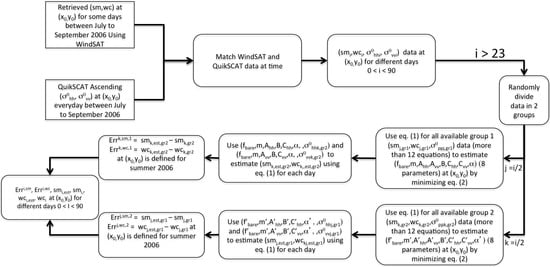
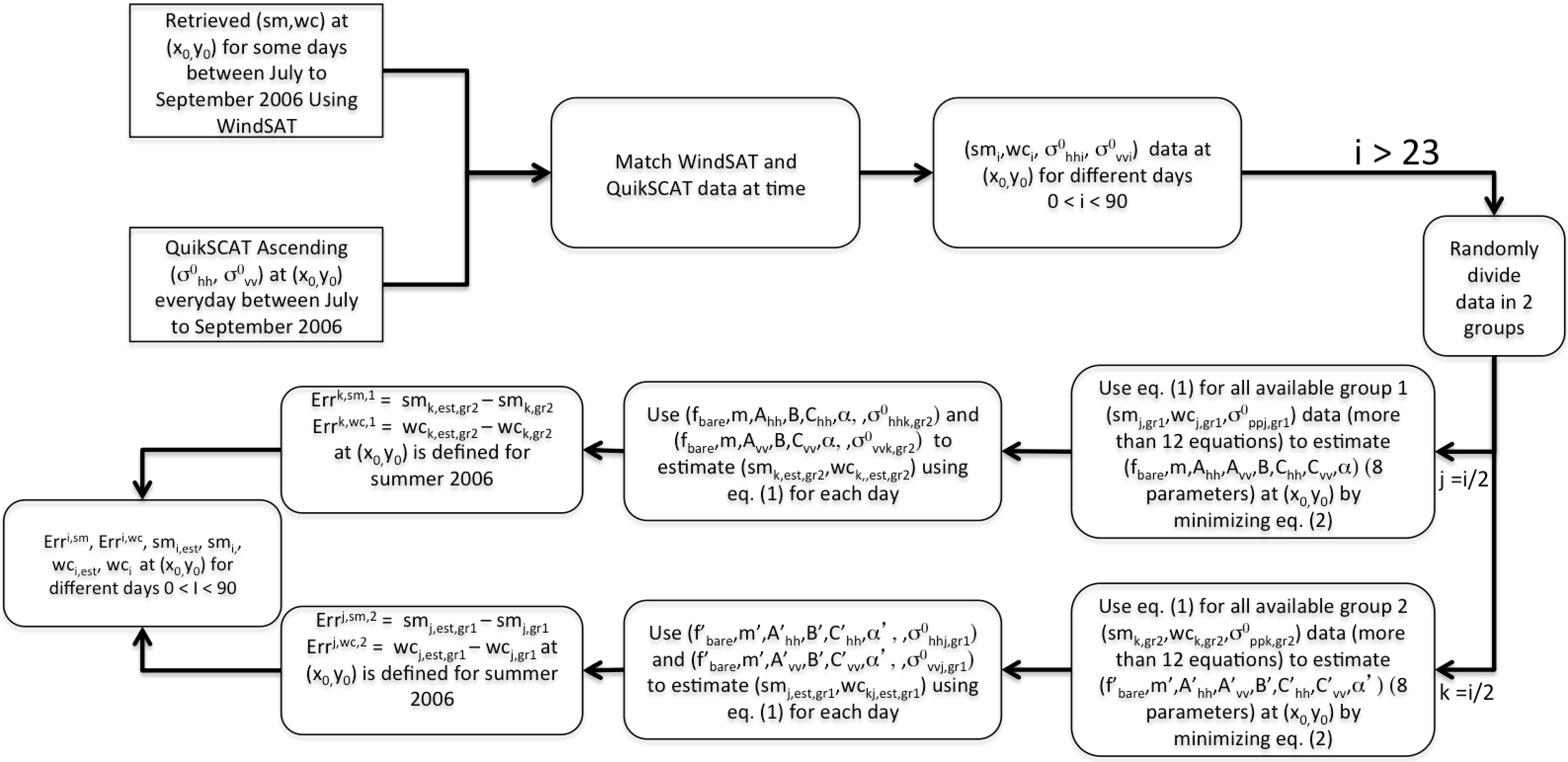
The goal of this study is to retrieve soil moisture and vegetation water content daily and globally during the summer season of 1999 to 2009. In Figure 1, different steps to retrieve soil moisture and vegetation water content using QuikSCAT data are explained. The 2006 data set is used in this study because it has the largest pool of retrieved WindSAT sm and wc during the summer season. The time series studies will be the future of this work. As explained in Figure 1, for each location on earth, there is a collection of ascending QuikSCAT data for every morning between July to September 2006. Simultaneous retrieved (sm, wc) using WindSAT data exist for a fraction of days during summer 2006. If more than 23 or samples are available during summer 2006, of that location are estimated as explained in Section 4.1. As explained in Section 4.2, a 2-folded cross-validation method is used for validation in this study. Note that, in this method, half of available data are randomly used for parameter estimation. The estimated parameters and the other half of QuikSCAT data are used to estimate as discussed in Section 4.2. The estimated are compared with the other half of WindSat . Therefore, half of the data are used for training and the other half are used for evaluating the model. In order to have equally good training and evaluation capabilities for our limited data, the data is partitioned into two “equal” sets.
4.1. Training the Backscattering Model for Each Location
As mentioned earlier, QuikSCAT L1B data sets with 25 km resolution are used in this study. The data covers almost the entire globe twice daily (ascending and descending). However, only the ascending observations are around the WindSat acquisition time. On the other hand, soil moisture (sm) and vegetation water content (wc) using WindSat data are retrieved [3]. The sm and wc data have gaps both spatially and temporally. The data is resampled to a global cylindrical EASE-Grid of 25 km resolution (true at 30° latitude). Therefore, for each point on the ease-grid coordinates, daily QuikSCAT (, ) data sets are available, whereas sm and wc are available for a portion of summer season.
For any point with available sm and wc, the are known variables and are unknown variables in Equation (1). Note that are known for each point on the ground. As explained earlier in Section 3, m contributes to the ground backscattering coefficient, contributes to vegetation backscattering, contributes to double bounce scattering of vegetation layer , and contributes to the attenuation of the vegetated layer. The sensitivity of the model to these parameters is analyzed in Section 5.3. Note that these unknown parameters are assumed to be constant during the summer compared to sm and wc. This is a reasonable assumption because the vegetation components (such as leave/branch size), rms height of the ground, and bare surface fraction vary very little during summer compared to soil moisture and vegetation water content. Therefore, for each point in a given day with available (sm, wc), there are two equations (Equation (1) for HH and VV) and eight unknowns. Hence, more observations are needed for each point to increase the number of equations. For the summer season of each year in the northern hemisphere, all eight unknown variables are assumed to remain constant and only sm and wc change. Therefore, at least four days with available are needed to have eight equations (for HH and VV polarizations). Using a 2-folded cross validation method (explained later in Section 4.2), half of the available data for each point is used to estimate eight parameters. The algorithm is set to apply to the points with at least 24 observations. Half of the available observations (i.e., 12 observations) are used for estimating eight unknowns to reduce the speckle noise error.
All retrieved WindSat and their instantaneous ascending QuikSCAT and are collected for each point during the summer season. Equation (1) is applied to () and (), assuming are the same for both polarizations. By minimizing
errors, all eight unknown parameters in Equation (1) are estimated for each point on the ground. There are n nonlinear equations and eight unknown parameters. We use the lsqnonlin function of MATLAB (version R2014a (8.3.0.532), MathWorks, Inc., USA) to estimate these eight parameters. The lsqnonlin function uses the trust-region-reflective algorithm to minimize the error in Equation (2). and in Equation (2) are the backscattered power in Equation (1) and ith observed QuikSCAT backscattered power, respectively. n is the number of observations for a specific point during summer season. Standard deviation of the observed mostly lies between 20 to 30% of its mean. Residual error defined by Equation (2), on the other hand, mostly lies between 2 to 4% of QuikSCAT mean value. Hence, the residual error of the fit to the observation is much smaller than the variation of the observation itself. Therefore, the model is a good fit to the observation.
For the ground backscattering coefficient () in Equation (1), Physical Optics (PO), Geometrical Optics (GO), Small Perturbation Model (SPM), and the model by Oh et al. (Oh) are examined [15,17]. Oh’s model performs better in terms of residual error. Therefore, the model by Oh et al. is used for the ground backscattering for the rest of this work. A better ground backscattering model in the Ku-band is needed for better quantification of ground backscattering.
4.2. Vegetation Water Content and Soil Moisture Retrieval Using QuikSCAT Backscattered Power Data
As discussed in Section 4.1, for each point on the ground, there are eight parameters that quantify backscattering power with respect to vegetation water content and soil moisture. Therefore, there is a predefined Equation (1) for each point on the ground with two unkowns (sm, wc). Two observations are needed to estimate sm and wc. As explained in Section 2.2, there are QuikSCAT and data sets twice daily and globally. Hence, for any points on the ground with the available eight parameters, soil moisture and vegetation water content are estimated in the morning and in the afternoon (corresponding to QuikSCAT ascending and descending data) during summer 2006. Note that WindSat data are no longer needed in this stage of sm and wc retrieval. WindSat data is only used to estimate different parameters in Equation (1). Using those parameters and QuikSCAT data, we can retrieve sm and wc and there is no need for WindSat data in the retrieval process. However, WindSat data is needed to evaluate retrieved sm and wc accuracy. On the other hand, part of the WindSat data is needed for estimating parameters in Equation (1) and separate parts for evaluating sm and wc retrieval.
The 2-folded cross-validation method is used to evaluate the performance of estimating soil moisture and vegetation water content. For each point on the ground, all the collocated WindSat and QuikSCAT data points are randomly divided to two sets, group one and group two, so that both sets are equal size. The eight parameters (or ) for group 1 (or 2) are estimated. Then, eight parameters from group 1 (or 2) are used to estimate sm and wc using group 2 (or 1) QuikSCAT backscattered data. Finally, the estimated sm and wc are compared with group 2 (or 1) WindSat sm and wc. The total error would be the average of these two groups’ errors. The details of this method are shown in Figure 1. This method has the advantage that both training and test sets are large, and each data point is used for both training and validation on each fold. However, at least eight equations are needed for each group of data to estimate eight parameters. A minimum of 12 available observations are considered for each group to increase the accuracy of the eight parameters’ estimation. The more points we use in our parameter estimation, the more accurate our results would be. There is a trade-off between minimum number of observations needed for each location to increase accuracy, and earth coverage of our estimation algorithm. Looking at the histogram of available observations for each location during summer 2016, we chose a minimum of 12 observations. Therefore, for each location on Earth, there need to be at least 24 observations during summer 2006 to perform 2-folded cross-validation.
Note that, by using the 2-folded cross validation method, half of co-located QuikSCAT and WindSat data (for each point) are used to train Equation (1). Then, the trained equation is used to estimate sm and wc using the other half of backscattered QuikSCAT data. The estimated sm and wc will be compared with the other half of WindSat data. Therefore, half of the data is used for training, whereas the other half is used for estimation and validation.
5. Results and Discussion
5.1. Temporal and Spatial Correlation of the Backscattering Model Parameters
In order to evaluate the stability of parameters in Equation (1), the spatial and temporal correlation of these parameters are calculated. Figure 2 shows the spatial correlation for different parameters in Equation (1). Note that the resolution of these parameters is 25 km (EASE-Grid resolution). We expect that some parameters in Equation (1) change relatively smoothly in both space and time. For instance, bare surface fraction is expected to vary smoothly in space and time (high spatial and temporal correlation), simply because no desert is observed next to a dense forest. Some other parameters are expected to vary relatively randomly in both space and time (low spatial and temporal correlation). For instance, varies relatively randomly in space and time because any orientation change of scatterers in time and space affects the backscattering coefficient. Since parameter retrieval of each pixel is independent of neighboring pixels, the high spatial correlation shows both the stability of the retrieval algorithm and the physical meaning of that parameter.
As seen in Figure 2, and have the highest spatial correlation. The spatial correlation for is about 0.6 for 200 km spatial distance, which means that the bare surface fraction changes very smoothly over the ground, as expected. Among the vegetation parameters, B has the highest spatial correlation. Parameter B is proportional to attenuation coefficient of the vegetation, whereas and depend on the direct backscattering coefficient and double bounce of the vegetation, respectively. Any orientation variation changes dramatically, while attenuation is more stable. Hence, the observed spatial correlations meet our expectations.
Parameters in Equation (1) are also estimated for summer of 2004. Table 1 lists the statistical comparison between the estimated parameters of 2006 and 2004. The first row shows the correlation between parameters in 2004 and 2006. Note that represents a specific parameter at year i. The second and third rows show the mean and standard deviation of differences between parameters at year 2004 and 2006 normalized to the mean of the parameter in percentile. The mean and standard deviation of the difference could be small/large because the parameter itself is small/large. Therefore, it is normalized to the mean of the parameter. As seen in this table, have high temporal correlation, and relatively small mean and standard deviation error. The vegetation parameters can change significantly with any environmental variable such as wind. Therefore, they show almost no correlation between 2004 and 2006. The stability of f and shows the model and our estimation algorithm is stable enough to use as a method to estimate the vegetation water content and soil moisture as explained in Section 4.2. Note that there is no claim that the parameters in the parametric formulation in Equation (1) are the most physically meaningful or, indeed, in any way the best parameters to use to describe the scattering from soil and vegetation.
5.2. Evaluating Bare Surface Fraction Estimation
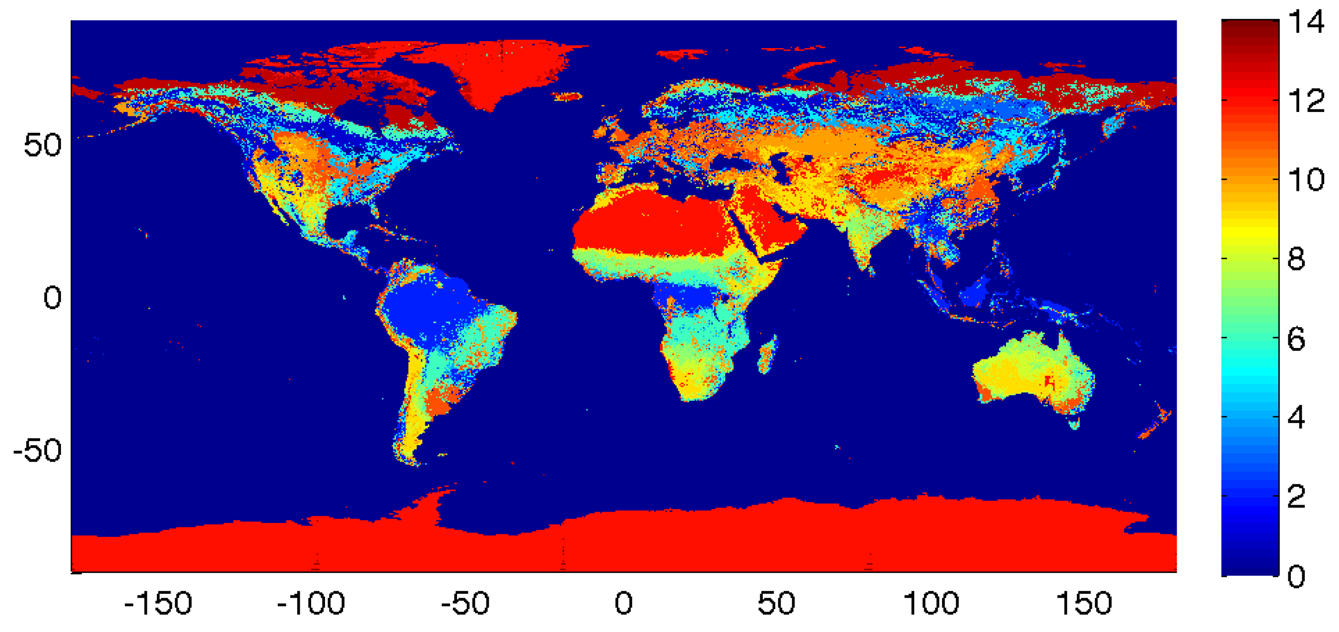
In order to study different areas based on the type of land coverage, a global map of land surface classification [22] is used as shown in Figure 3.
Bare surface fraction, , is the only parameter in Equation (1) that can be easily compared with in situ measurements. Other parameters in Equation (1), such as , , and , depend on scattering from the trees and are difficult to measure. In this study, the bare surface fraction estimates using MODerate-resolution Imaging Spectroradiometer (MODIS) data are used. The Vegetation Continuous Fields (VCF) collection contains proportional estimates for vegetative cover types: woody vegetation, herbaceous vegetation, and bare ground [23]. The product is derived from all seven bands of the MODIS sensor onboard NASA’s Terra satellite. This VCF product shows how much of a land cover such as “forest” or “grassland” exists anywhere on a land surface. The resolution of the data is 210 m; therefore, 96 pixels are averaged to match the 20 km resolution of QuikSCAT.
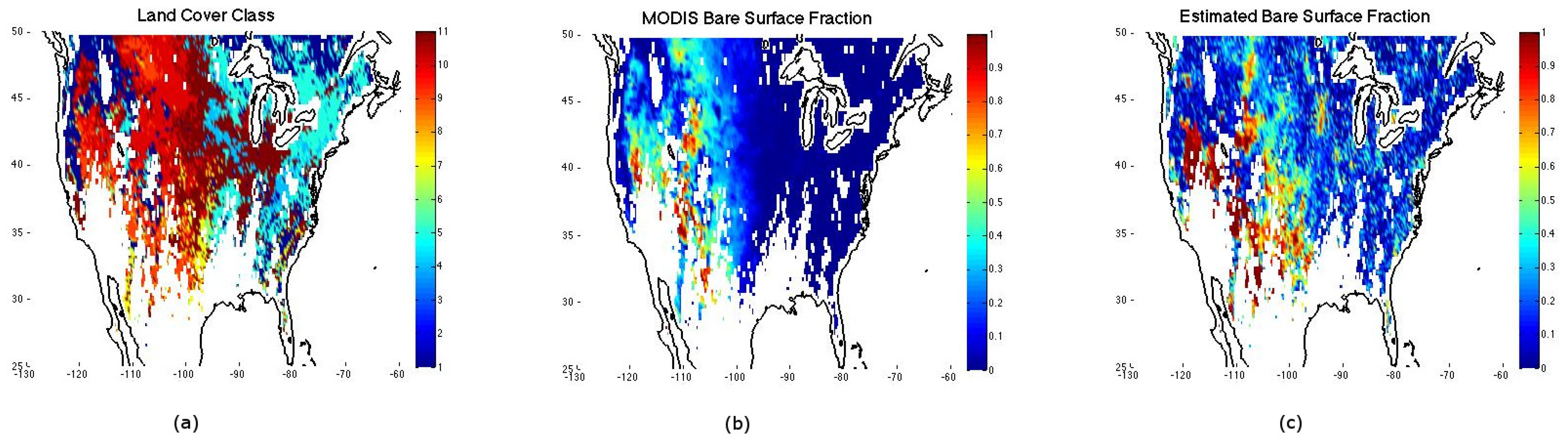
Figure 4a shows the land cover classes over the U.S. Figure 4b shows the bare surface fraction using 2001 MODIS data [23]. The bare surface fraction estimate using our algorithm in Section 4.1 and 2006 WindSat and QuikSCAT data is shown in Figure 4c. The bare surface fraction data using 2006 MODIS data is under processing [23]. The bare surface fraction is expected to change but remain correlated between 2001 and 2006. Hence, we expect that areas with relatively high/low bare surface fractions in 2001 (like Amazon/deserts as two extremes) have relatively high/low bare surface fraction in 2006. As seen in Figure 4, our estimate of bare surface fraction looks similar to estimates using MODIS data.
The correlation between data in Figure 4b,c for different classes is shown in Table 2. The number of samples in class 2 is small; hence, no correlation value is assigned to class 2 in Table 2.
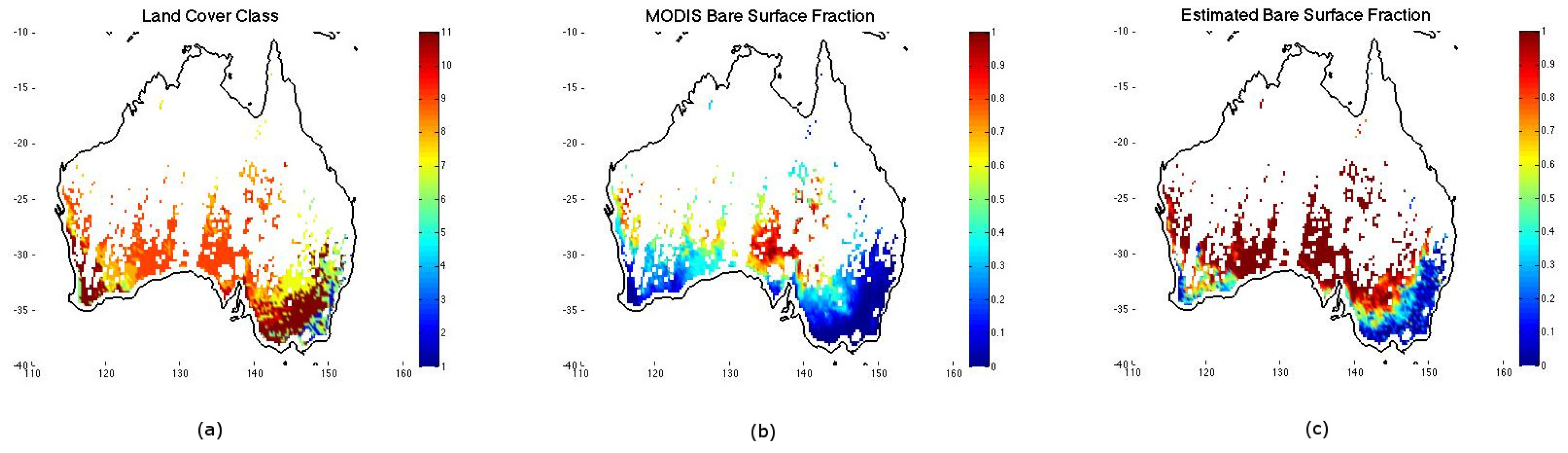
Figure 5a–c is the same as Figure 4 but over Australia. Note that the data used in Figure 5 are between July to September 2006 (winter season in the southern hemisphere). The low correlations in non-forested regions is most likely due to snow cover. The global correlation between estimates of bare surface fraction using MODIS and QuikSCAT is shown in the last row of Table 2.
As can be seen in this table, the correlation between MODIS and QuikSCAT estimates of bare surface fraction is very low over forested areas and relatively high over non-forested areas. This could be due to the shadow of forests over bare surface areas because of a radar look angle of greater than 50°. Although the direct return below vegetation cover is neglected in the Ku-band, no shadowing effect is considered in our model. On the other hand, backscattering from trees dominates the total backscattering in forested areas, which affects the accuracy of bare surface fraction estimates. The relatively high global correlation over classes 7, 9, and 10 suggests good estimates of bare surface fraction over no-branch (leafy) regions. We define "no-branch" regions as areas with soft leaves and no hard branches such as grassland and open shrubland regions. Although closed shrublands (class 8) are non-forested regions, they have small branches that may decrease the accuracy of estimation. However, open shrublands (class 9) show a better performance. Therefore, a better estimate of bare surface fraction is obtained over no-branch areas as the branches block the returns from the ground in the Ku-band. Similarly, croplands (class 11) in the summer season reduce the bare surface fraction estimates by blocking the Ku-band return from the ground. The shadowing effect of branches could be the reason for poor bare surface fraction estimation, but more investigation is needed to better explain the observed correlations in Table 2 and the fact that branches decrease the accuracy of bare surface fraction estimates.
The estimated bare surface fraction using QuikSCAT saturates quickly as it increases. As increases, the backscattering from vegetation increases, whereas the backscattering from the ground decreases. Because of the small wavelength of the Ku-band, any small vegetation cover blocks the ground return. Therefore, the estimated bare surface fraction is biased towards larger values. More investigation is needed to better evaluate the reason for this saturation. Because of the saturation problem, the mean and standard deviations of bare surface fraction estimate error are not shown here. However, the general resemblance between the bare surface fraction using MODIS and QuikSCAT in Figure 4b,c is promising.
5.3. Sensitivity Analysis
In this section, the sensitivity of HH and VV polarization backscattered power is evaluated with different parameters in Equation (1). The mean value of each parameter is used to calculate the backscattered power using Equation (1). The mean values used in this equation are (0.176, 0.028, 0.1, 0.05, 0.2, 0.021,0.35) for (), respectively. is calculated to quantify the sensitivity of backscattered power to parameter K by
Table 3 shows the sensitivity of backscattered power to different parameters considering .
As seen in this table, the variation of is less than 10% with changing any parameter by 20%. This means that the relative change in is less than the relative change in any parameter by at least a factor of 2. Therefore, the model is pretty stable with respect to different parameters’ variations. The model is most sensitive to , but is almost stable with respect to other parameters’ variation. However, is more sensitive to bare surface fraction and soil moisture. Therefore, the proposed model is in general very stable to any parameter variations.
5.4. Comparing Retrieved Vegetation Water Content and Soil Moisture Using QuikSCAT and WindSat Based on Land Surface Classification
As described above, for every point with minimum 24 points of collocated WindSat and QuikSCAT data, vegetation water content and soil moisture are estimated everyday during the summer. Note that all errors and coherence comparisons in this section are based on 2-folded cross-validation method explained in Section 4.2.
Table 4 shows statistical comparison between retrieved sm and wc using our estimation method and WindSat sm and wc, for different classes. Note that there are very few observations for classes 3, 12, and 13 to show any statistical comparison. Row 2 shows the correlation between all retrieved wc using QuikSCAT and WindSat during summer 2006 at a specific class. There is a good correlation (greater than 0.4) between retrieved wc using QuikSCAT and WindSat for classes 1, 2, 4, 5, 6, 7, 10, and 11. A correlation greater than 0.4 is considered high enough in this study to show a relationship between two variables. Open and closed shrublands (classes 8 and 9) have low correlation. Rows 4 and 6 show the mean and standard deviation of the wc retrieval error (using the 2-folded cross-validation method) as a percentage of the mean of wc. As seen in this table, the mean of wc retrieval error is very small for all classes except classes 8 and 9, similar to the correlation pattern. The standard deviation of wc retrieval error (row 6) has almost the same pattern as row 4. However, the standard deviation is around 50% for all classes except 8 and 9. Hence, our vegetation water content retrieval algorithm performs well for classes 1 to 7 and 11, and reasonably for class 10. The performance is poor for classes 8 and 9.
Row 3 in Table 4 shows the correlation between retrieved soil moisture using QuickSCAT and WindSat for different classes. The correlation between retrieved soil moisture using QuikSCAT data and WindSat is in general very low. The coherence increases as the land class changes from forested to bare surface, probably due to less ground backscattered power blocked by the trees in the Ku-band. For the forested areas, there is almost no correlation between retrieved soil moisture using QuikSCAT and WindSat because the return from the ground is very weak. Rows five and seven show the mean and standard deviation of sm retrieval error (using a 2-folded cross-validation method) compared to the mean of sm, in percent, during summer 2006. As can be seen in this table, the mean and std of sm retrieval error is lower for lower classes, which is not consistent with correlation values (row 3). Therefore, the sm retrieval performs poorly based on land surface classification.
Note that, if the retrieved values are averaged for each location to reduce the speckle noise, the coherence between vegetation water content using Windsat and QuikSCAT increases to more than 0.8 and standard deviation decreases to less than 7% for classes 1 to 5. On the other hand, there could be a delay between the time vegetation water content appearing in QuikSCAT and Windsat. Averaging removes this kind of time lag and shows better performance of our retrieval algorithm.
5.5. Comparing Retrieved Vegetation Water Content and Soil Moisture Using QuikSCAT and WindSat Based on Bare Surface Fraction
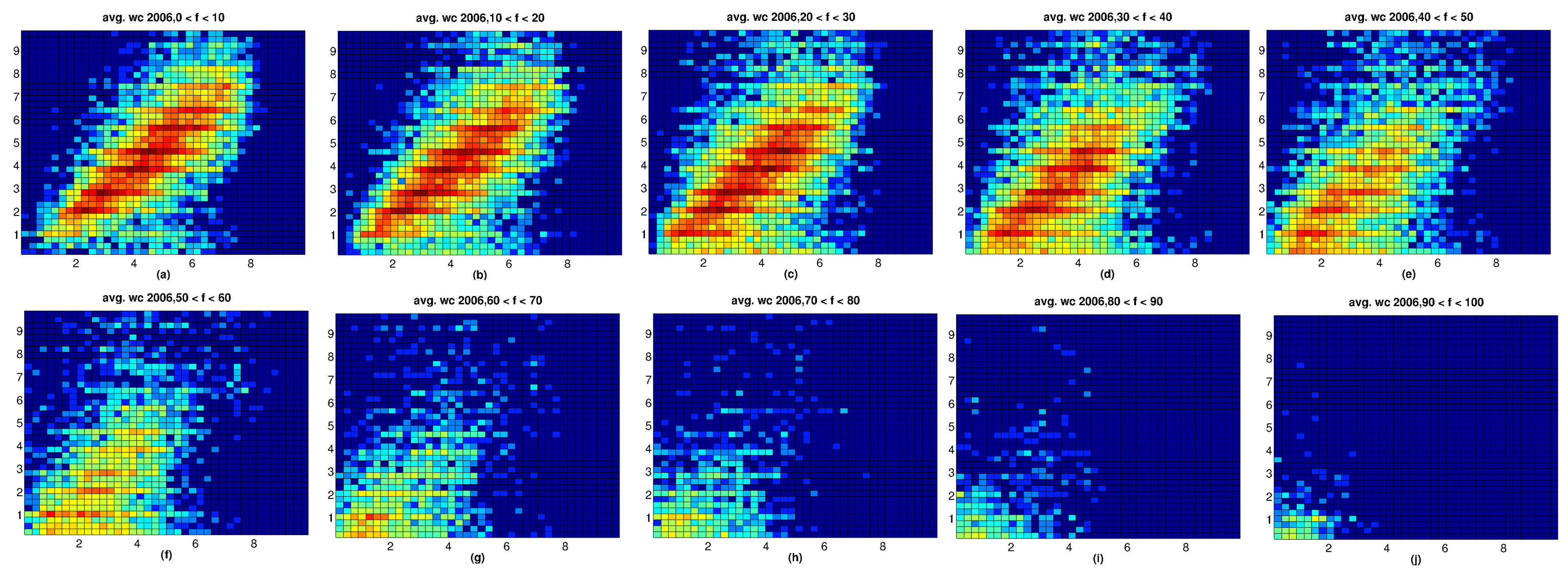
The bare surface fraction is used in this section for classifying the performance of sm and wc retrieval algorithms. Figure 6 shows the retrieved wc using QuikSCAT data versus retrieved wc using WindSat data over summer 2006 for different retrieved bare surface fractions () (based on a 2-folded cross validation method). As seen in this figure, in areas with small bare surface fraction, there is a good linear relationship between wc using QuikSCAT and WindSat. As the bare surface fraction increases, the data cloud in Figure 6 spreads more. This is due to the fact that backscattering from the ground dominates. Therefore, the accuracy of estimated wc decreases as expected.
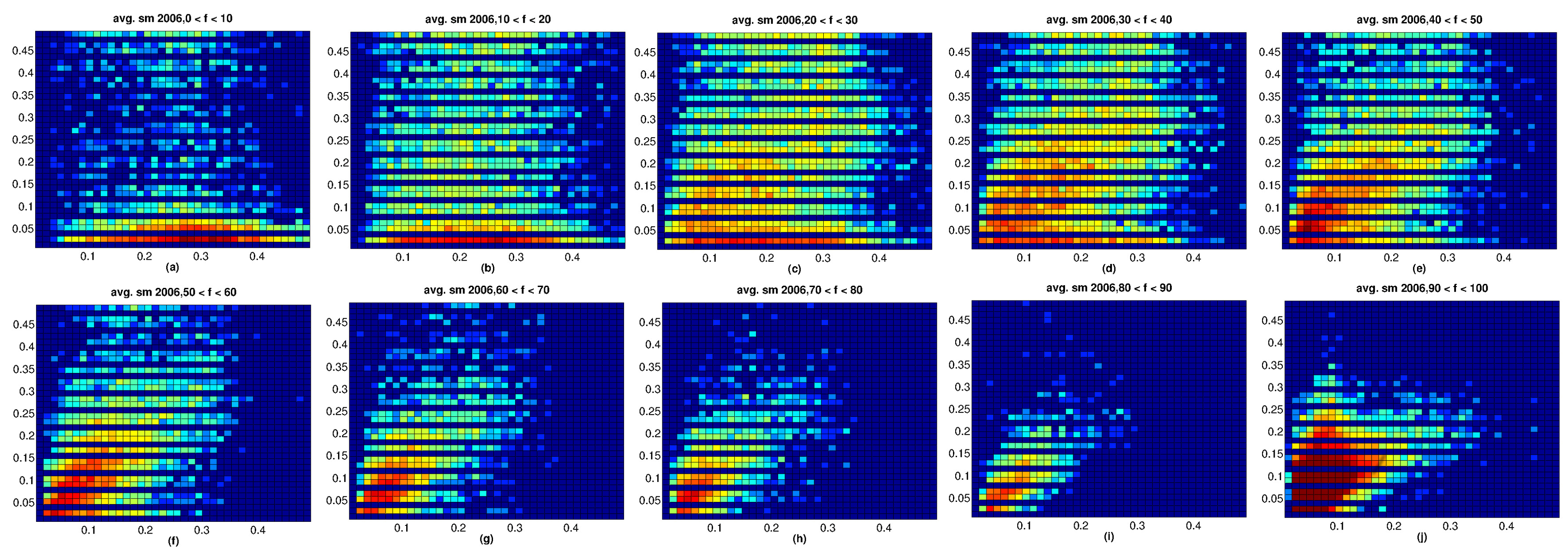
Figure 7 shows the retrieved sm using QuikSCAT data versus retrieved sm using WindSat data for different retrieved bare surface fractions () (based on 2-folded cross-validation method). Figure 7 separates well the regions with poor and good performance in soil moisture retrieval. As seen in Figure 7a,b, the sm retrieval performs very poorly in regions with a small bare surface fraction. However, as the bare surface fraction increases in Figure 7c to g, a better estimate of soil moisture is achieved, as expected. The statistical performance of retrieved algorithm is summarized in Table 5. Note that the number of points in areas with high bare surface fraction is larger in Figure 7 compared to Figure 6. This is due to the fact that the model is limited to ground backscattering (first term in Equation (1)) if the WindSat wc is very small.
Table 5 shows statistical comparison between retrieved sm and wc using QuikSCAT and WindSat for different bare surface fractions based on 2-folded cross-validation method. Different columns in this table correspond to different bare surface fractions. Comparing the performance statistics of retrieved wc in Table 4 and Table 5, one could see that land surface classes better separates regions with good and bad performances. Mean and std of retrieved wc error (rows 4 and 6) for regions with good retrieval performances (low bare surface fraction in Table 5 and forested regions in Table 4) are larger in Table 5 than Table 4. Therefore, land surface class is suggested to be used to classify regions with good vegetation water content retrieval.
Comparing Table 4 and Table 5, it is observed that bare surface fraction better separates regions with good and bad sm retrieval than land surface classification. As shown in Figure 7 and also row 3 of Table 5, the correlation between retrieved sm using WindSAT and QuikSCAT increases as bare surface fraction increases. Note that the coherence values for large bare surface fraction in row 3 of Table 5 are much larger than coherence values for less forested areas (larger land classes) in row 3 of Table 4. The mean and std of sm retrieval error (rows 5 and 7) compared to mean of sm decrease as bare surface fraction increases (for bare surface fraction more than 50%). Hence, rows 3, 5, and 7 are consistent for bare surface fractions larger than 50%. Therefore, our soil moisture retrieval algorithm performs well for large bare surface fractions but poorly for low bare surface fractions, as expected. For regions with bare surface fraction larger than 90%, the retrieved algorithm works poorly for low soil moisture ranges. More investigation is needed to discover the relatively poor soil moisture retrieval for > 90%.
Note that retrieved sm using QuikSCAT shows good correlation (more than 0.4) with retrieved sm using WindSat for large bare surface fractions, as seen in Figure 7 and Table 5. However, the standard deviation of retrieved sm error is relatively large. This observation suggests that either any vegetation decreases the sensitivity of the Ku-band to soil moisture or the backscattering model from the ground is not appropriate in the Ku-band. Moran et al. [24] also showed that, although Ku-band backscattered power is sensitive to ground roughness in agricultural crops, it is independent from soil moisture. However, it is shown that retrieved soil moisture is correlated enough to the actual values. More investigation is needed to determine the reason for the high standard deviation.
Note that, if the retrieved values are averaged for each location to reduce the speckle noise, the correlation between soil moisture using Windsat and QuikSCAT increases to more than 0.8 and standard deviation decreases to less than 28% for bare surface fraction less than 60%. On the other hand, there could be a delay between the time soil moisture appearing in QuikSCAT and Windsat. The averaging also reduces the effect of time lag.
6. Conclusions
A backscattering formulation in the Ku-band is proposed in this work. Estimating soil moisture and vegetation water content using already available QuikSCAT Ku-band backscattered power data is shown for the first time in this study. Estimated bare surface fraction and vegetation attenuation coefficient show high spatial and temporal correlation, as expected. However, the estimated bare surface fraction using QuikSCAT saturates quickly as it increases and the reason should be more investigated. There is also a high correlation (more than 0.5) between bare surface fraction using MODIS and QuikSCAT for no-branch regions in the U.S. More investigation is needed to better explain the reason that branches decrease the accuracy of bare surface fraction estimates. Scattering coefficients in Equation (1), on the other hand, show low spatial and temporal correlation. These parameters change with wind (direction of scattering elements) or other environmental variations.
The backscattering formula with known parameters for each location on Earth is then used to retrieve soil moisture and vegetation water content using HH and VV QuikSCAT backscattered power, daily and globally. There is a good agreement (based on 2-folded cross validation method) between retrieved vegetation water content using WindSat and QuikSCAT, especially for forest classes where vegetation is the main contributor in the backscattering power in the Ku-band. Using the bare surface fraction as a classifying parameter, a good agreement (correlation greater than 50% for bare surface fraction greater than 60%) between retrieved soil moisture using WindSat and QuikSCAT is observed for areas with high bare surface fraction. This is due to the fact that ground backscattering is the main contributor to total backscattered power.
This study shows the potential of using already available QuikSCAT data to estimate vegetation water content globally twice a day. The QuikSCAT data are available daily and globally from 1999 to 2009. The trained backscattered formulation for each location can be applied to QuikSCAT data. Hence, the QuikSCAT 1999-2009 data could produce a big library of retrieved vegetation water content to investigate the effect of climate change on vegetation in this period. Improving our estimate of soil moisture could help other missions such as SMAP (Soil Moisture Active Passive). Fusion of Ku-band RapidScat data and L-band SMAP data for producing more accurate soil moisture and vegetation water content is the future of this study. The time series of retrieved vegetation water content and soil moisture map from 1999 to 2009 is being analyzed and will be the subject of a future paper.
Acknowledgments
The authors would like to thank all the reviewers for their useful comments. The research was carried out at the Jet Propulsion Laboratory, California Institute of Technology, under a contract with the National Aeronautics and Space Administration.
Author Contributions
Ziad Haddad conceived and designed the original plan for the empirical algorithm to retrieve soil moisture and vegetation water content from scatterometer observations using a reference database of coincident retrievals from WindSat. Shadi Oveisgharan built the algorithm, performed all the analyses and validation, and wrote the paper. Joe Turk helped with providing the bare surface fraction. Ernesto Rodriguez provided critical guidance on the validation. Li Li provided the WindSat retrievals.
Conflicts of Interest
The authors declare no conflict of interest.
References
- Saatchi, S.; Halligan, K.; Despain, D.G.; Crabtree, R.L. Estimation of Forest Fuel Load from Radar Remote Sensing. IEEE Trans. Geosci. Remote Sens. 2007, 45, 1726–1740. [Google Scholar] [CrossRef]
- Saatchi, S.; Asefi-Najafabady, S.; Malhi, Y.; Aragao, L.; Anderson, L.; Myneni, R.; Nemani, R. Persistent effects of a severe drought on Amazonian forest canopy. PNAS 2013, 110, 565–570. [Google Scholar] [CrossRef] [PubMed]
- Li, L.; Gaiser, P.W.; Gao, B.C.; Bevilacqua, R.M.; Jackson, T.J.; Njoku, E.G.; Rudiger, C.; Calvet, J.C.; Bindlish, R. WindSat Global Soil Moisture Retrieval and Validation. IEEE Trans. Geosci. Remote Sens. 2010, 48, 2224–2241. [Google Scholar] [CrossRef]
- Moghaddam, M.; Saatchi, S.; Cuenca, R.H. Estimating subcanopy soil moisture with radar. J. Geophys. Res. 2000, 105, 14899–14911. [Google Scholar] [CrossRef]
- Roo, R.D.; Du, Y.; Ulaby, F.T. A semi-empirical backscattering model at L-band and C-band for a soybean canopy with soil moisture inversion. IEEE Trans. Geosci. Remote Sens. 2001, 39, 864–872. [Google Scholar] [CrossRef]
- Kim, S.B.; Moghaddam, M.; Tsang, L.; Burgin, M.; Xu, X.; Njoku, E.G. Models of L-Band Radar Backscattering Coefficients Over Global Terrain for Soil Moisture Retrieval. IEEE Trans. Geosci. Remote Sens. 2014, 52, 1381–1396. [Google Scholar] [CrossRef]
- Kim, S.B.; Arii, M.; Jackson, T. Modeling L-Band Synthetic Aperture Radar Data Through Dielectric Changes in Soil Moisture and Vegetation Over Shrublands. IEEE J. Sel. Top. Appl. Earth Obs. Remote Sens. 2017, 10, 4753–4762. [Google Scholar] [CrossRef]
- Bruscantini, C.A.; Konings, A.G.; Narvekar, S.; McColl, K.A.; Entekhabi, D.; Grings, F.M.; Karszenbaum, H. L-Band Radar Soil Moisture Retrieval without Ancillary Information. IEEE J. Sel. Top. Appl. Earth Obs. Remote Sens. 2015, 8, 5526–5540. [Google Scholar] [CrossRef]
- Ouellette, J.D.; Johnson, J.T.; Balenzano, A.; Mattia, F.; Satalino, G.; Kim, S.B.; Dunbar, R.S.; Colliander, A.; Cosh, M.H.; Caldwell, T.G.; et al. A Time-Series Approach to Estimating Soil Moisture From Vegetated Surfaces Using L-Band Radar Backscatter. IEEE Trans. Geosci. Remote Sens. 2017, 55, 3186–3193. [Google Scholar] [CrossRef]
- Yang, L.; Du, H.; Zhao, J.; Liu, Q. Global Vegetation Dynamic Monitoring using Multiple Satellite Observations, 2002–2007. In Proceedings of the 2011 IEEE International Geoscience and Remote Sensing Symposium (IGARSS), Vancouver, BC, Canada, 24–29 July 2011; pp. 771–774. [Google Scholar]
- Mladenova, I.; Lakshmi, V.; Walker, J.; Long, D.G.; Jeu, R.D. An Assessment of QuikSCAT Ku-Band Scatterometer Data for Soil Moisture Sensitivity. IEEE Geosci. Remote Sens. Lett. 2009, 6, 640–643. [Google Scholar] [CrossRef]
- Zec, J.; Jones, W.L.; Long, D.G. SeaWinds beam and slice balance using data over Amazonian rainforest. Proc. IGARSS 2000, 5, 2215–2217. [Google Scholar]
- Long, D.G.; Drinkwater, B.H.; Saatchi, S.; Bertoia, C. Global ice and land climate studies using scatterometer image data. EOS Trans. AGU 2001, 82, 503. [Google Scholar] [CrossRef]
- Kunz, L.B.; Long, D.G. Calibrating SeaWinds and QuikSCAT scatterometers using natural land targets. IEEE Geosci. Remote Sens. Lett. 2005, 2, 182–186. [Google Scholar] [CrossRef]
- Ulaby, F.T.; Moore, R.K.; Fung, A.K. Microwave Remote Senising, Active and Passive; Artech House, Inc.: Norwood, MA, USA, 1981. [Google Scholar]
- Saatchi, S.; McDonald, K.C. Coherent Effects in Microwave Backscattering Models for Forest Canopies. IEEE Trans. Geosci. Remote Sens. 1997, 35, 1032–1044. [Google Scholar] [CrossRef]
- Oh, Y.; Sarabandi, K.; Ulaby, F. An Empirical Model and an Inversion Technique for Radar Scattering from Bare Soil Surfaces. IEEE Trans. Geosci. Remote Sens. 1992, 30, 370–381. [Google Scholar] [CrossRef]
- Hallikainen, M.T.; Ulaby, F.; Dobson, M.C.; El-Rayes, M.A.; Wu, L. Microwave Dielectric Behavior of Wet Soil-Part 1: Empirical Models and Experimental Observations. IEEE Trans. Geosci. Remote Sens. 1985, 23, 25–34. [Google Scholar] [CrossRef]
- Cloude, S.R.; Papathanassiou, K.P. Polarimetric SAR Interferometry. IEEE Trans. Geosci. Remote Sens. 1998, 36, 1551–1565. [Google Scholar] [CrossRef]
- Papathanassiou, K.P.; Cloude, S.R. Single-Baseline Polarimetric SAR Interferometry. IEEE Trans. Geosci. Remote Sens. 2001, 39, 2352–2362. [Google Scholar] [CrossRef]
- Reynolds, C.A.; Jackson, T.J.; Rawls, W.J. Estimating soil water-holding capacities by linking the Food and Agriculture Organization Soil map of the world with global pedon databases and continuous pedotransfer functions. Water Resour. Res. 2000, 36, 3653–3662. [Google Scholar] [CrossRef]
- Hansen, M.; DeFries, R.; Townshend, J.; Sohlberg, R. Global land cover classification at 1km resolution using a decision tree classifier. Int. J. Remote Sens. 2000, 21, 1331–1365. [Google Scholar] [CrossRef]
- DiMiceli, C.; Carroll, M.; Sohlberg, R.; Huang, C.; Hansen, M.; Townshend, J. Vegetation Continuous Fields; University of Maryland: College Park, MD, USA, 2010. [Google Scholar]
- Moran, M.S.; Vidal, A.; Troufleau, D.; Inoue, Y.; Mitchell, T.A. Ku- and C-Band SAR for Discriminating Agricultural Crop and Soil Conditions. IEEE Trans. Geosci. Remote Sens. 1994, 36, 265–272. [Google Scholar] [CrossRef]
Figure 1.
Flow chart showing the steps for 2-folded cross-validation in retrieving soil moisture and vegetation water content.
Figure 1.
Flow chart showing the steps for 2-folded cross-validation in retrieving soil moisture and vegetation water content.
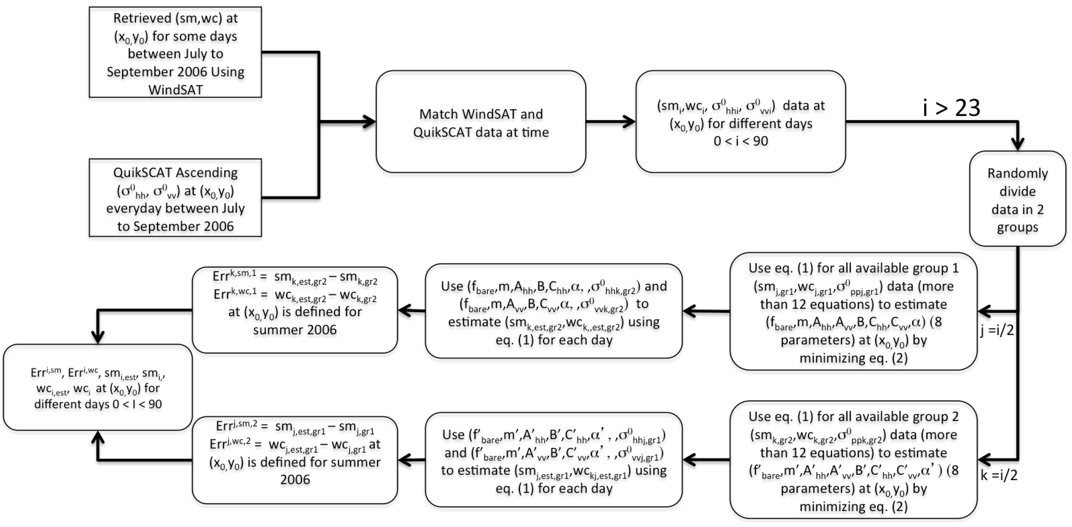
Figure 2.
Spatial correlation of different parameters in our backscattered power formulation.
Figure 3.
Global map of different classes of the Earth’s surface. 0: Water, 1: Evergreen Needleleaf Forest, 2: Evergreen Broadleaf Forest, 3: Deciduous Needleleaf Forest, 4: Deciduous Broadleaf Forest, 5: Mixed Forest, 6: Woodland, 7: Wooded Grassland, 8: Closed Shrubland, 9: Open Shrubland, 10: Grassland, 11: Cropland, 12: Bare Ground, 13: Urban and Built classes are shown by different colors changing from dark blue to dark red.

Figure 4.
(a) land cover classes map of the U.S.; (b) 2001 bare surface fraction map of the U.S.; (c) estimated bare surface fraction map of the U.S.
Figure 4.
(a) land cover classes map of the U.S.; (b) 2001 bare surface fraction map of the U.S.; (c) estimated bare surface fraction map of the U.S.

Figure 5.
(a) land cover classes map of Australia; (b) 2001 bare surface fraction map of Australia; (c) estimated bare surface fraction map of Australia.
Figure 5.
(a) land cover classes map of Australia; (b) 2001 bare surface fraction map of Australia; (c) estimated bare surface fraction map of Australia.

Figure 6.
2D logarithmic histogram of retrieved vegetation water content (kg/m2) using QuikSCAT backscattered power vs. estimated vegetation water content using WindSat data for all the points around the globe over month of summer 2006 for bare surface fraction of (a) 0 < f < 15%; (b) 15 < f < 30%; (c) 30 < f < 45%; (d) 45 < f < 60%; (e) 60 < f < 75%; (f) 75 < f < 85%; (g) 85 < f < 90%; (h) 90 < f < 100%.

Figure 7.
2D logarithmic histogram of retrieved soil moisture (m3/m3) using QuikSCAT backscattered power vs. estimated soil moisture using WindSat data for all the points around the globe over summer 2006 for bare surface fraction of (a) 0 < f < 15%; (b) 15 < f < 30%; (c) 30 < f < 45%; (d) 45 < f < 60%; (e) 60 < f < 75%; (f) 75 < f < 85%; (g) 85 < f < 90%; (h) 90 < f < 100%.


Table 1.
Statistical comparison of 2004 and 2006 parameters. K is the parameter specified above each column.
Table 1.
Statistical comparison of 2004 and 2006 parameters. K is the parameter specified above each column.
| m | f | |||||||
|---|---|---|---|---|---|---|---|---|
| Temporal correlation of and | 0.17 | 0.73 | 0.17 | 0.3 | 0.33 | 0.41 | 0.14 | 0.24 |
| 2.2 | 1.7 | 42.9 | 20.7 | 20.2 | 9.3 | 38.1 | 27.1 | |
| 125 | 55 | 304 | 163 | 153 | 71 | 307 | 203 |
Table 2.
Correlation between bare surface fraction using 2001 MODIS data and bare surface fraction estimate using our algorithm in Section 4.1 and summer of 2006 QuikSCAT and WindSat data over the U.S. and Australia for different classes.
Table 2.
Correlation between bare surface fraction using 2001 MODIS data and bare surface fraction estimate using our algorithm in Section 4.1 and summer of 2006 QuikSCAT and WindSat data over the U.S. and Australia for different classes.
| Land Class Defined in Figure 3 | 1 | 2 | 4 | 5 | 6 | 7 | 8 | 9 | 10 | 11 |
|---|---|---|---|---|---|---|---|---|---|---|
| correlation between f using | ||||||||||
| MODIS and QuikSCAT over U.S. | 0.18 | −0.04 | −0.01 | 0.31 | 0.46 | 0.53 | 0.57 | 0.54 | 0.38 | |
| correlation between f using | ||||||||||
| MODIS and QuikSCAT over Australia | 0.16 | 0.7 | 0.54 | 0.37 | 0.2 | 0.65 | 0.73 | |||
| correlation between f using | ||||||||||
| MODIS and QuikSCAT globally | 0.15 | 0.05 | −0.02 | 0.08 | 0.14 | 0.48 | 0.23 | 0.38 | 0.62 | 0.3 |
Table 3.
Sensitivity of and to 20% variation of parameters in columns 2 to 9, respectively.
| 3.9481 | 3.3357 | 3.9843 | 3.6804 | 9.2442 | 3.1523 | 4.5713 | 2.1570 | |
| 6.7795 | 2.2424 | 3.4495 | 2.8116 | 7.4456 | 2.5390 | 6.9394 | 1.5846 |
Table 4.
Statistical behavior of vegetation water content/soil moisture retrieval during summer 2006 for different classes.
Table 4.
Statistical behavior of vegetation water content/soil moisture retrieval during summer 2006 for different classes.
| Row 1 | Land Class | 1 | 2 | 4 | 5 | 6 | 7 | 8 | 9 | 10 | 11 |
| Row 2 | correlation between wc of QuikSCAT and WindSat | 0.55 | 0.5 | 0.5 | 0.52 | 0.41 | 0.47 | 0.21 | 0.19 | 0.4 | 0.42 |
| Row 3 | correlation between sm of QuikSCAT and WindSat | 0.11 | 0.1 | 0.12 | 0.03 | 0.22 | 0.25 | 0.31 | 0.33 | 0.43 | 0.21 |
| Row 4 | 2.6 | −3.5 | 0.8 | 0.7 | −0.3 | 1.1 | 68.4 | 40.5 | 16.7 | 3.9 | |
| Row 5 | 4.2 | 9.5 | 1.6 | -2.4 | 36.6 | 53.7 | 40.6 | 30.3 | 30.1 | 24.8 | |
| Row 6 | 54.1 | 43.6 | 51.8 | 50 | 60 | 72.4 | 221.4 | 219.9 | 116.1 | 67.7 | |
| Row 7 | 83.6 | 86.5 | 88.9 | 79.3 | 116.3 | 142.4 | 127 | 124.5 | 136.5 | 106 |
Table 5.
Statistical behavior of vegetation water content/soil moisture retrieval during summer 2006 for different bare surface fractions.
Table 5.
Statistical behavior of vegetation water content/soil moisture retrieval during summer 2006 for different bare surface fractions.
| Row 1 | Bare Surface Fraction (%) | 0–10 | 10–20 | 20–30 | 30–40 | 40–50 | 50–60 | 60–70 | 70–80 | 80–90 | 90–100 |
| Row 2 | correlation between wc of QuikSCAT and WindSat | 0.6 | 0.56 | 0.49 | 0.43 | 0.44 | 0.37 | 0.34 | 0.3 | 0.26 | 0.12 |
| Row 3 | correlation between sm of QuikSCAT and WindSat | −0.06 | 0.06 | 0.17 | 0.25 | 0.38 | 0.46 | 0.5 | 0.57 | 0.62 | 0.51 |
| Row 4 | 2.2 | 2.6 | 3.2 | 3.5 | 4.1 | 5.5 | 12.3 | 22.4 | 30.8 | 66.6 | |
| Row 5 | 2.3 | 14.1 | 18.1 | 24.2 | 25.9 | 27.6 | 26.9 | 18.3 | 11.4 | 10.6 | |
| Row 6 | 41.5 | 47.9 | 59.1 | 70.4 | 78.4 | 92.4 | 114.4 | 148.7 | 183.3 | 277.7 | |
| Row 7 | 99.2 | 101.4 | 97.9 | 98.3 | 97.9 | 96.4 | 95.5 | 84.3 | 75 | 80.4 |
© 2018 by the authors. Licensee MDPI, Basel, Switzerland. This article is an open access article distributed under the terms and conditions of the Creative Commons Attribution (CC BY) license (http://creativecommons.org/licenses/by/4.0/).
Share and Cite
MDPI and ACS Style
Oveisgharan, S.; Haddad, Z.; Turk, J.; Rodriguez, E.; Li, L. Soil Moisture and Vegetation Water Content Retrieval Using QuikSCAT Data. Remote Sens. 2018, 10, 636. https://doi.org/10.3390/rs10040636
AMA Style
Oveisgharan S, Haddad Z, Turk J, Rodriguez E, Li L. Soil Moisture and Vegetation Water Content Retrieval Using QuikSCAT Data. Remote Sensing. 2018; 10(4):636. https://doi.org/10.3390/rs10040636
Chicago/Turabian StyleOveisgharan, Shadi, Ziad Haddad, Joe Turk, Ernesto Rodriguez, and Li Li. 2018. "Soil Moisture and Vegetation Water Content Retrieval Using QuikSCAT Data" Remote Sensing 10, no. 4: 636. https://doi.org/10.3390/rs10040636
Note that from the first issue of 2016, this journal uses article numbers instead of page numbers. See further details here.