Influence of Tropical Instability Waves on Phytoplankton Biomass near the Marquesas Islands


1
University of Brest, Ifremer, CNRS, IRD, Laboratoire d’Océanographie Physique et Spatiale (LOPS), IUEM, 29200 Brest, France
2
IRD, UPF, ILM, Ifremer, Écosystèmes Insulaires Océaniens (EIO), 98702 Tahiti, French Polynesia
3
Laboratoire de Géosciences du Pacifique Sud, Université de la Polynésie française, 98702 Tahiti, French Polynesia
*
Author to whom correspondence should be addressed.
Remote Sens. 2018, 10(4), 640; https://doi.org/10.3390/rs10040640
Submission received: 21 March 2018
/
Revised: 13 April 2018
/
Accepted: 16 April 2018
/
Published: 20 April 2018
(This article belongs to the Special Issue Remote Sensing of Ocean Colour)
Abstract
:The Marquesas form an isolated group of small islands in the Central South Pacific where quasi-permanent biological activity is observed. During La Niña events, this biological activity, shown by a net increase of chlorophyll-a concentration (Chl, a proxy of phytoplankton biomass), is particularly strong. It has been hypothesized that this strong activity is due to iron-rich waters advected from the equatorial region to the Marquesas by tropical instability waves (TIWs). Here we investigate this hypothesis over 18 years by combining satellite observations, re-analyses of ocean data, and Lagrangian diagnostics. Four La Niña events ranging from moderate to strong intensity occurred during this period, and our results show that the Chl plume within the archipelago can be indeed influenced by such equatorial advection, but this was observed during the strong 1998 and 2010 La Niña conditions only. Chl spatio-temporal patterns during the occurrence of other TIWs rather suggest the interaction of large-scale forcing events such as an uplift of the thermocline or the enhancement of coastal upwelling induced by the tropical strengthening of the trades with the islands leading to enhancement of phytoplankton biomass within the surface waters. Overall, whatever the conditions, our analyses suggest that the influence of the TIWs is to disperse, stir, and, therefore, modulate the shape of the existing phytoplankton plume.
1. Introduction
Over the next century, the frequency of extreme La Niña events is expected to nearly double from one in every 23 years to one in every 13 years [1]. In the Pacific Ocean, a La Niña event induces an increase of phytoplankton biomass along the eastern and central equatorial/tropical band through the uplift of the thermocline and hence of nutrients [2,3,4,5], but also more locally around islands [6,7,8,9,10]. In such an island context, biological variability can be directly influenced by local processes such as land drainage, dust deposition, changes occurring at basin/regional scale (i.e., basin-scale thermocline depth and wind variability), and/or can be impacted by remote forcing, such as the horizontal advection of cold nutrient-rich waters upwelled along the Equator due to tropical instability waves (TIWs) [11,12,13]. Tropical instability waves are cusp-shaped oceanic perturbations of currents and temperature [14]. They are generated either by the baroclinic instability associated with sea surface temperature (SST) fronts or the barotropic instability associated with the ocean current shears between the eastward Equatorial Undercurrent (EUC) and the opposing westward flowing South Equatorial Current (SEC) [15]. During La Niña events, the trade winds drive the enhancement of the equatorial currents, hence, TIW activity is maximized [16].
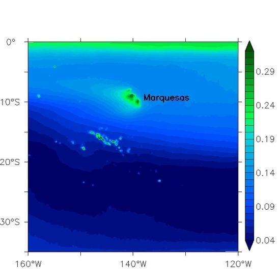
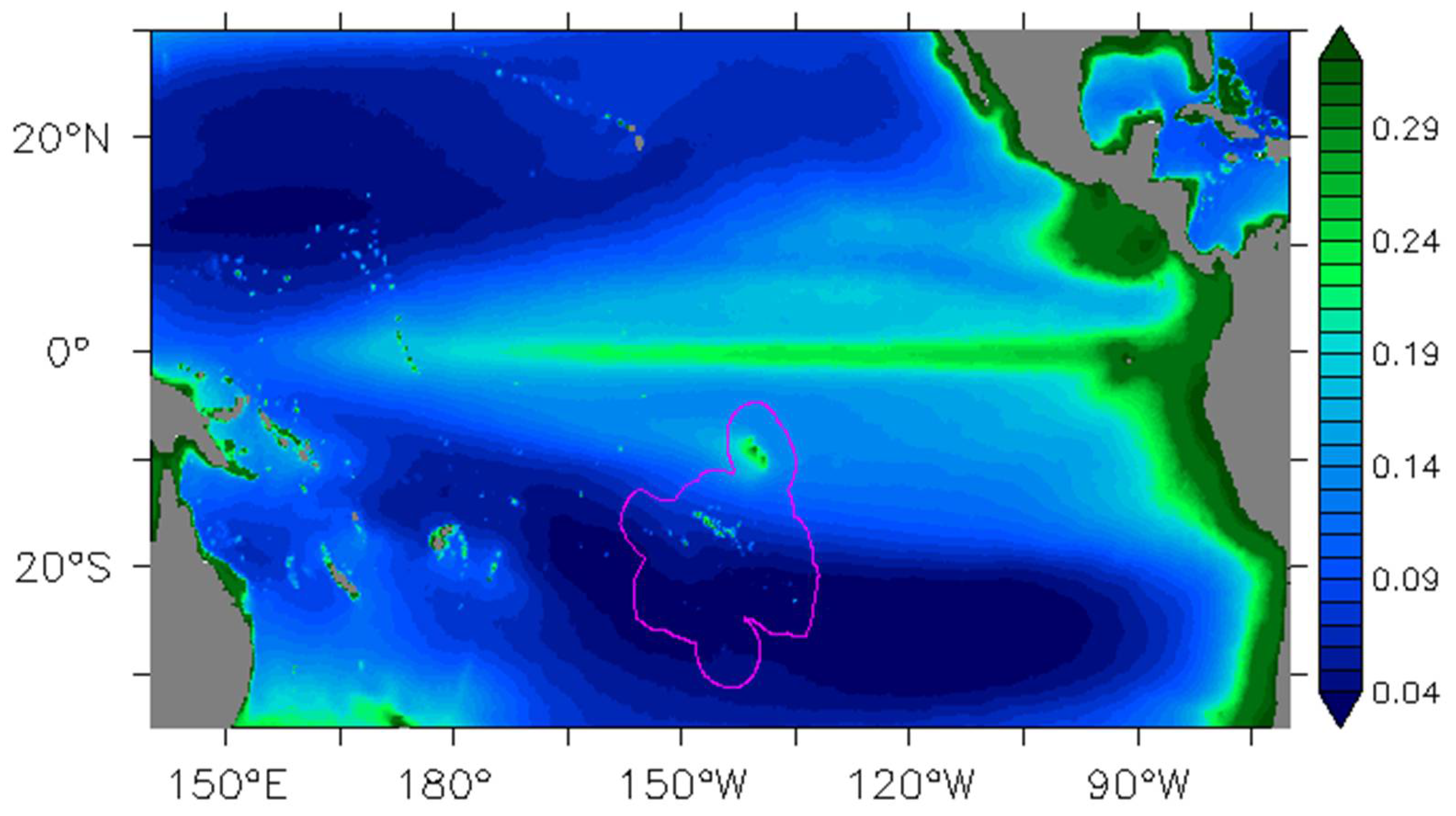
The Marquesas islands are located in the Central South Pacific (11°S–8°S/142°W–139°W) in high nutrient low chlorophyll (HNLC) waters south of the equatorial upwelling region (Figure 1). HNLC waters present some moderate oligotrophic characteristics associated with significant amounts of nitrate ([17] and references therein). The archipelago extends over about 350 km and islands rise steeply from the abyssal plain at 4000 m. Hence, deep channels between the islands (40 to 100 km wide) allow the SEC to flow unobstructed south-westward, while the dozens of islands themselves divert the flow as they are 10–25 km-wide obstacles embedded in the SEC. A strong biological enhancement referred to as an island mass effect (IME, [18]) occurs in the location of these small islands. An annual mean of 0.2 mg/m3 of surface chlorophyll-a concentration (Chl, a proxy of phytoplankton biomass) has been reported [19]. The authors also reported a strong correlation between this IME and the total (Ekman plus geostrophic) surface current. However, the relevant process at the origin of the blooms was not identified. During La Niña events in 1998 and 2000, Chl rose to 0.3 and 0.5 mg/m3, respectively. The 1998 Chl increase was associated with a plume extending up to 800 km in the lee of the islands [6]. To explain the phytoplankton enhancement during the 1998 La Niña event, two hypotheses have been proposed. Firstly, it could be attributed to local sources of iron and the interactions of the Marquesas with the La Niña-enhanced SEC [6,19]. Secondly, a progression of cooler bands of equatorial waters that extend far to the south and can reach the Marquesas islands has been associated with TIW fronts [7]. Hence, these authors have suggested that the upwelled equatorial waters rich in iron generating phytoplankton blooms could be advected downstream along TIWs.
This second hypothesis has been proposed for 1998 only, a year when a strong La Niña event occurred [7]. Hence, here we investigate the consistency of this hypothesis over a longer period (18 years) and under different La Niña conditions. In order to detect TIWs and to follow their propagations, we used satellite observations combining ocean colour, SST, altimetric surface currents and fronts, and transport barrier information derived from altimetric surface currents, along with estimates of the density field issued from a re-analysed ocean model.
2. Materials and Methods
We used the Chl AVE GlobColour data set developed, validated, and distributed by ACRI-ST France [20,21,22]. This product merges derived-Chl from L3 Ocean Colour products derived from four different sensors (Sea-viewing Wide Field-of-view Sensor, Moderate Resolution Imaging Spectroradiometer Aqua, Medium-Resolution Imaging Spectrometer, and Visible Infrared Imaging Radiometer Suite) to produce a long-time series with a better spatio-temporal coverage than that provided by each individual ocean colour mission. Weekly surface data, from September 1997 to December 2014, were available on a 4-km horizontal grid.
Sea surface temperature was used to detect the cold water associated with TIWs. Data were provided by the AVHRR Pathfinder Project v4.1 (1985–2002) and AVHRR GAC (2003–present) [23]. Weekly data on a 9 km horizontal grid were downloaded for the 1997–2014 period [24].
In order to investigate the possible pathways and connectivity between the Equator and the Marquesas islands and, hence, the possible surface advection of phytoplankton or iron-rich waters by TIWs, we used passive Lagrangian diagnostics, with Finite-Size Lyapunov Exponents (FSLEs), derived from ocean surface currents (e.g., [25]). Finite-size lyapunov exponents enable us to study the relative dispersion between initially close particles, thus providing information on fronts and transport barriers, and on horizontal stirring by surface currents. Finite-size lyapunov exponents provided by AVISO+ [26] every 4 days on a 1/25° horizontal grid were derived from delayed-time global ocean absolute geostrophic currents (DUACS2014 DT MADT UV products). Parameters of the FSLE computations were defined to characterize the mesoscale features of the flow with an initial separation of 0.04 degrees and final separation of 0.6 degrees. We assumed here that FSLEs are representative of convergent structures and small-scale fronts that are relevant for the biological conditions and Chl variability [27,28,29].
Surface density was used to identify the signature of the TIW waters around the Marquesas archipelago. Surface density was provided daily from January 1998 to December 2012 by the ocean reanalyses from the HYbrid Coordinate Ocean Model (HYCOM; the more precise values originating from the GLBu0.08/expt_19.1 experiment, [30]) at the 1/12° horizontal resolution.
Finally, in order to demonstrate a possible arrival of the equatorial particles at the Marquesas, Lagrangian trajectories were directly calculated using satellite derived surface current velocities. The Ocean Surface Current Analysis Real-time (OSCAR) data set was provided every 5 days with a 1/3° spatial resolution [31]. A fourth-order Runge–Kutta technique was used to integrate the Lagrangian equations. The south-westward SEC was considered, and after some trials, it clearly appears that the water particles that could reach the Marquesas area come from the north-east. Hence, water particle departure points were taken every degree over the area 4°S–1°S/130°W–120°W. Since we were interested in knowing whether particles can reach the Marquesas and contribute to the local phytoplankton enhancement, the maximum time drift of the particles was chosen from 30 to 120 days. The shorter duration is the minimum time to drift from the Equator to the archipelago. The longer one is assumed to be just long enough for the equatorial iron and phytoplankton to be consumed and grazed, respectively. Particles were launched every five days and the number of particles within the Marquesas area (11°S–8°S/142°W–138°W) after the maximum time drift (corresponding to the chosen simulation) was recorded.
3. Results
3.1. The Case of the 1998 La Niña event
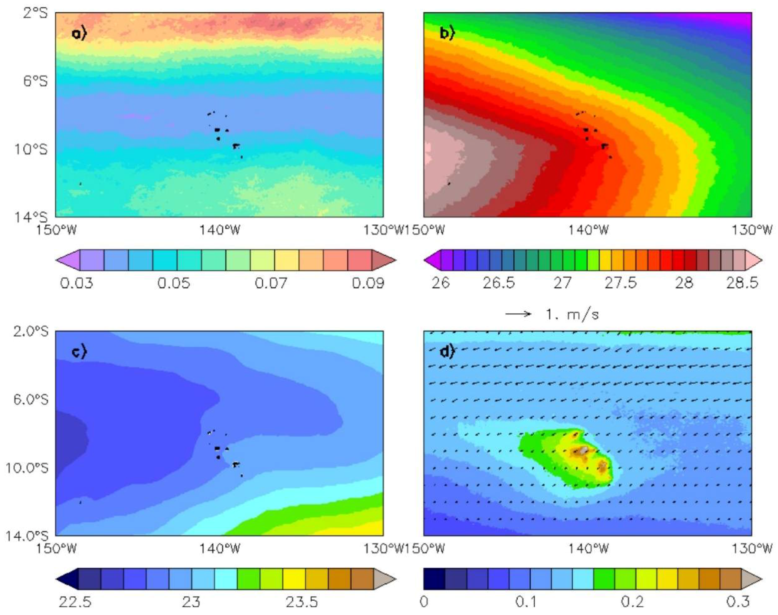
Finite-size lyapunov exponents were first used to identify large-scale regions characterized by different dynamical regimes. The 1998–2014 mean FSLE shows a weak dynamical activity area over 9°S–6°S/150°W–130°W, contrasting with the two higher dynamical regions located in the north along the Equator, and south of 10°S (Figure 2a). The Marquesas archipelago lies within the calm area where fronts and transport barriers are barely noticeable. From a dynamical point of view, the Marquesas area is associated with weaker surface currents, warmer and lighter waters than waters flowing from the equatorial region northeast of the islands (Figure 2b–d). The boundary of the oligotrophic and mesotrophic areas is noticeable southwest of the archipelago with low Chl (<0.1 mg/m3; Figure 1 and Figure 2d).
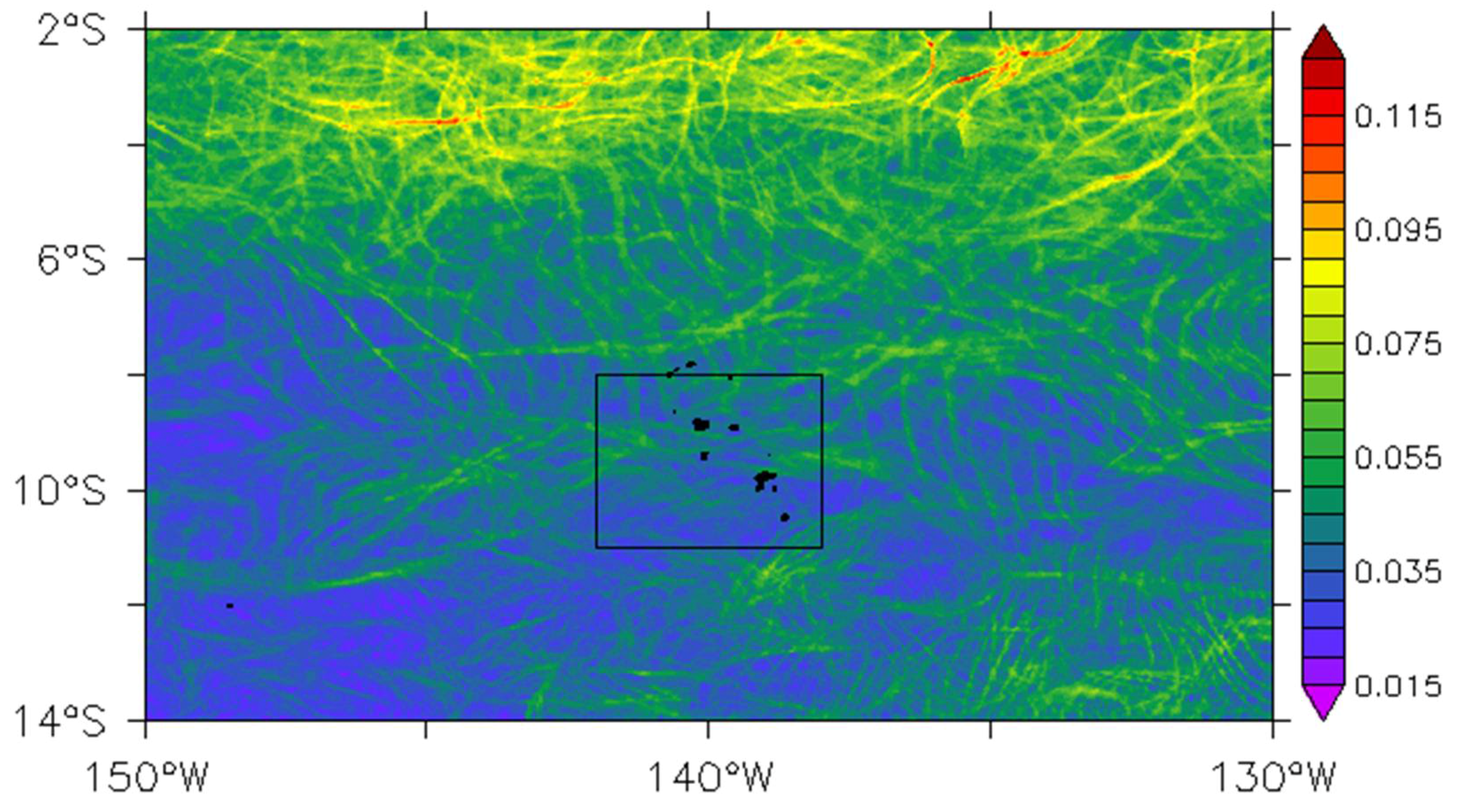
However, the weak dynamical activity within the Marquesas can be temporarily disrupted such as during the strong 1998–1999 La Niña. During this event, the FLSE annual root mean square (RMS) shows several individual paths of fronts induced by horizontal transport crossing the archipelago (Figure 3). This disturbance in the FSLE dynamic could be attributed to the intrusion of TIWs in 1998 as reported by Legeckis et al. [7].
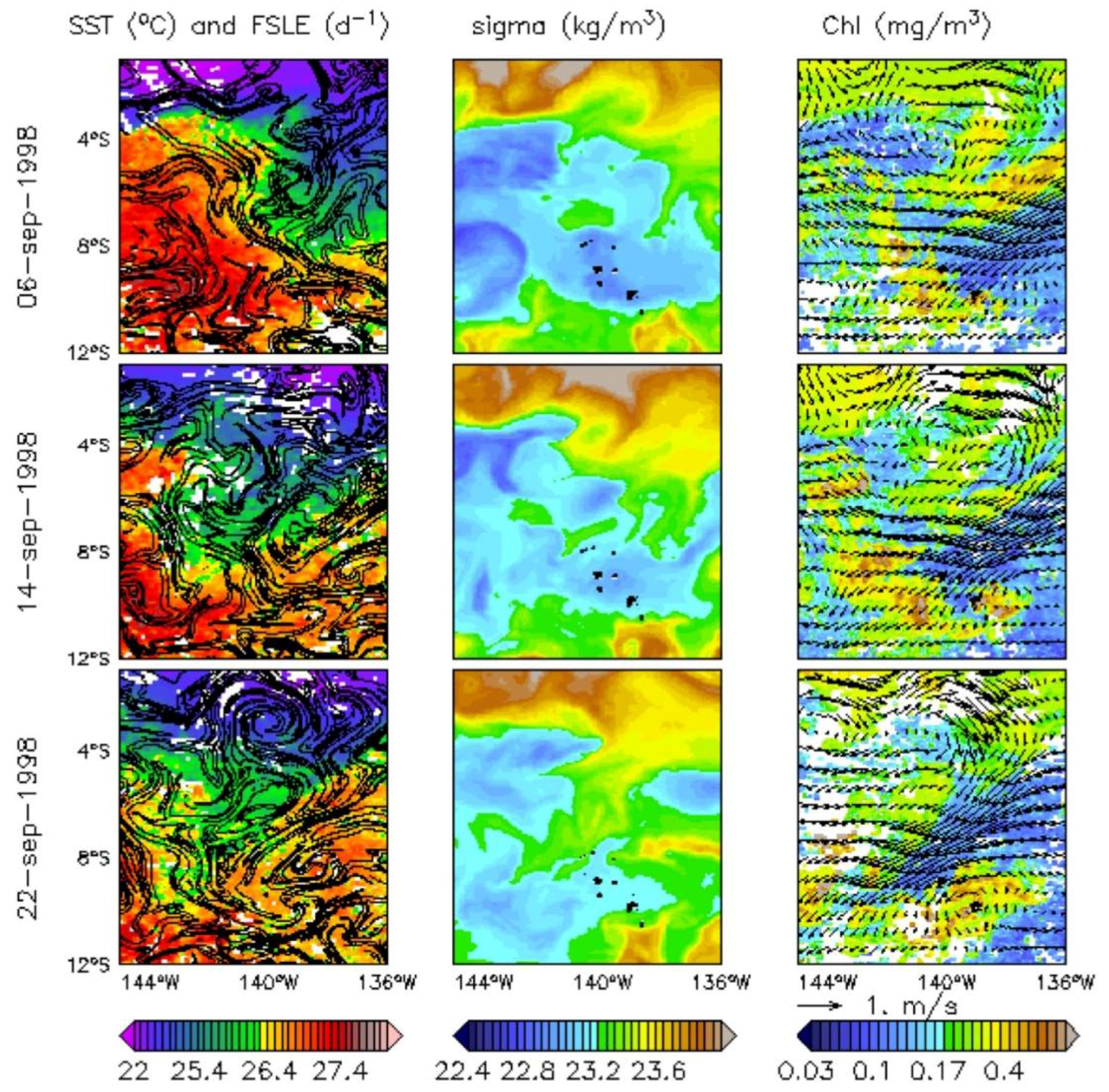
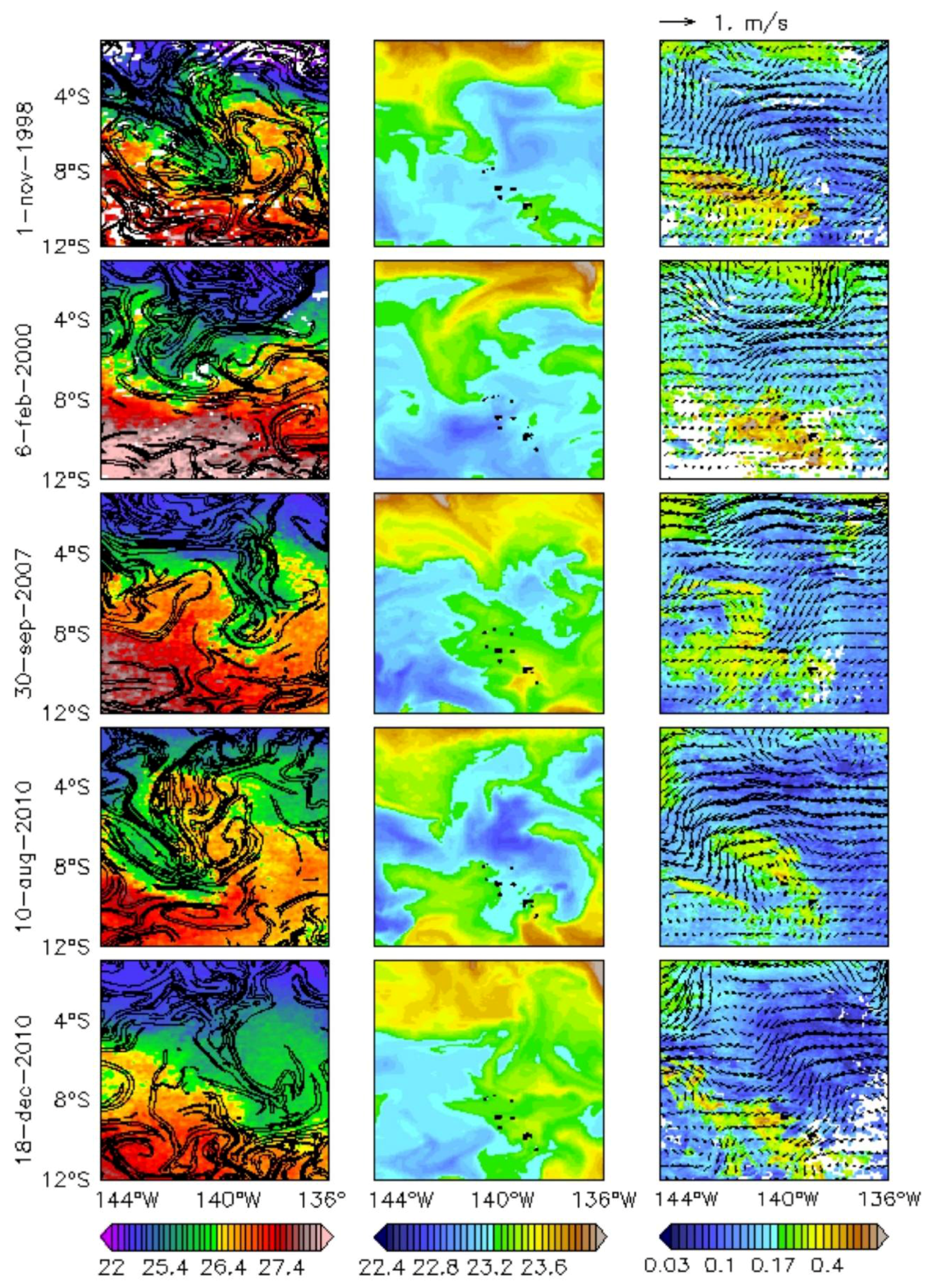
The particular event occurring in September 1998 illustrates how one of these TIWs reaches the archipelago along a north-east/south-west axis in association with low SST (as in Legeckis et al. [7]), a well-marked FSLE (Figure 4, left column), and high-density waters flowing from the Equator (Figure 4, centre column). This intrusion is most evident on 22 September 1998. Along the Equator, the highest Chl values (Figure 4, right column) are associated with SST approximately lower than 23 °C. Within the archipelago, a Chl plume was already noticeable prior to the arrival of the TIW (not shown), likely due to the IME. However, the equatorial band seems to be connected to the northern islands of the Marquesas through a region of strong FSLE gradient and higher Chl pathway than the surrounding waters. This higher Chl plume down to 8°S could be associated with an uptake of nutrient which is likely to reach the northern part of the archipelago. The eastern boundary of the region of strong gradient of FSLE is delimited by strong surface currents, associated with low Chl patterns. Not only is there is no apparent increase of Chl in this part of the archipelago, but the outer area of the TIW is associated with a stirred low Chl plume. This pattern also reflects the differences between the interior and the exterior of the TIW in terms of Chl, SST, and surface density.
3.2. Investigating the 1997–2014 Period
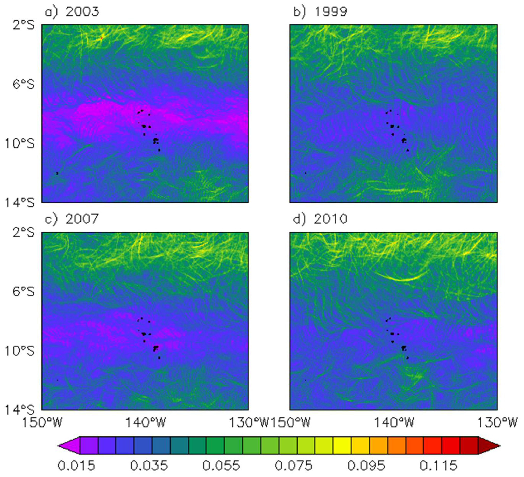
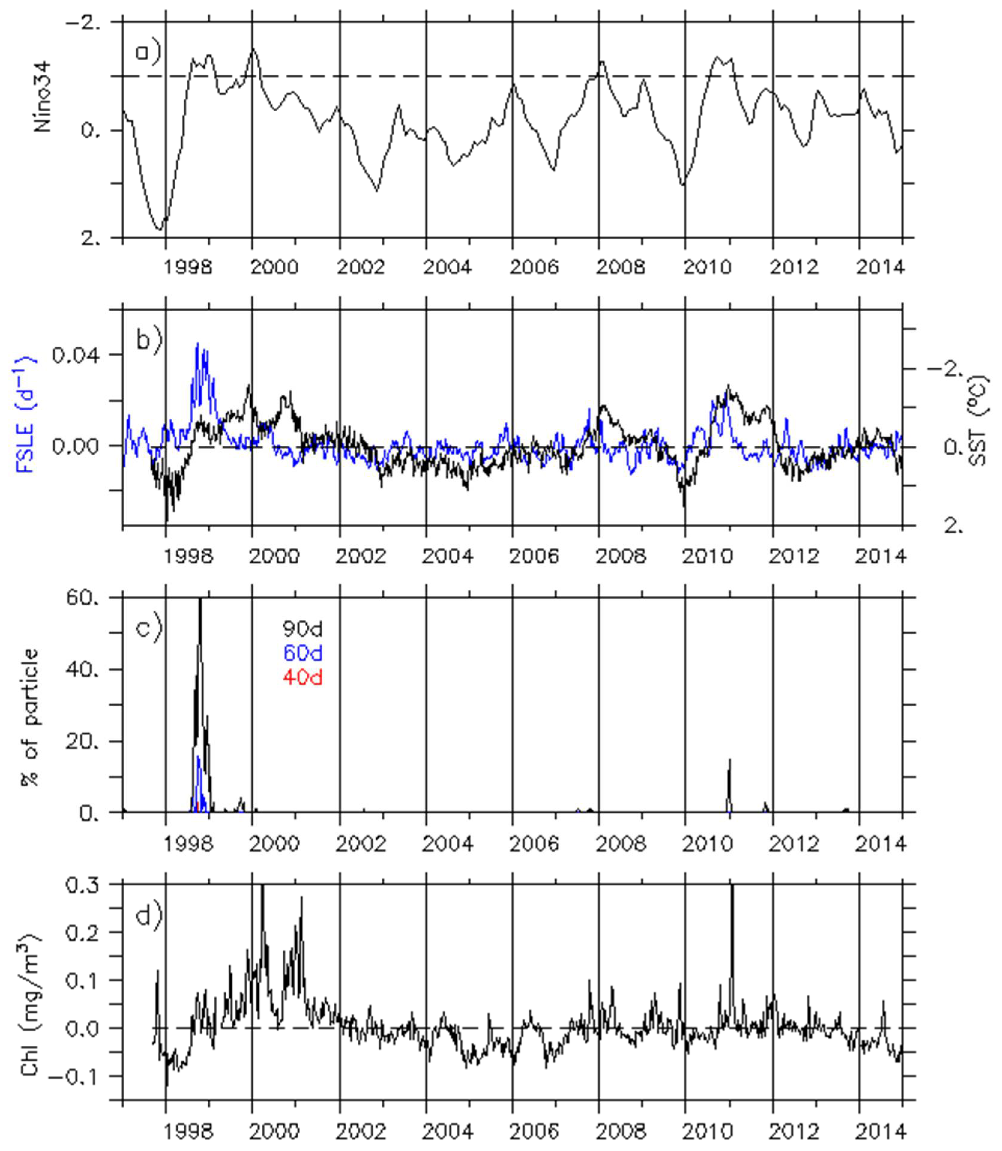
Considering the annual RMS values, FLSEs also have a characteristic signal in the Marquesas archipelago during other moderate to strong La Niña years (Figure 5). Consistently, the FSLE monthly anomalies (FSLEano) averaged over the archipelago (11°S–8°S and 142°W–138°W) are negatively correlated with the El Niño Southern Oscillation (ENSO) (rEl Nino34-FSLEano = −0.42; p < 0.001; Figure 6b blue line vs. Figure 6a). The weak dynamical activity within the archipelago is typical of neutral and El Niño years while during moderate to strong La Niña years (as defined with an index threshold of −1 in Figure 6a), the FSLE activity increases. SST monthly anomalies (SSTano) in this area are also correlated with ENSO (rEl Nino34-SSTano = 0.73; p < 0.001; Figure 6b black line). During La Niña events, when the equatorial cold tongue and the related current shear are intense, TIWs become unusually vigorous (e.g., [32,33]). Hence, cold anomalies associated with a high FSLE activity could be consistent with the passage of TIWs through the archipelago. However, the FSLEano increase within the archipelago is not solely related to the strength of La Niña events. Indeed, FSLEano is stronger in late 1998 than in 1999, 2008, or 2010, while SSTano is weaker and the El Niño 3.4 index is similar over these four years.
To further investigate the possibility of equatorial particles reaching the Marquesas, Lagrangian drift simulations were set up. After 30 days of drift, no particle reached the archipelago. It appears that the 1998 La Niña event is rather unique. Indeed, most particles reached the area after 40 to 60 days of drift for this 1998 event (Figure 6c). During the 2010 La Niña event some particles reached the archipelago after 3 to 4 months. These Equator–Marquesas connections in 1998 and 2010 can be related to the two strongest peaks in FSLE activity and TIW pathways.
According to Legeckis et al., an enhancement of the Marquesas IME should be expected [7]. However, Chl monthly anomalies (Chlano) increase only moderately following the FSLE and particle arrival in 1998, while the increase in 2010 is much stronger. The two strongest Chlano increases occurred around March 2000, and from mid-2000 to the beginning of 2001, strong and moderate La Niña years, respectively. While high Chlano in March 2000 might be related with a heavy rain event and induced island run-off, there is no explanation for the strong increase occurring in the end of 2000 [19]. However, in both cases these Chlano increases do not seem to be related with FSLE (and hence TIW) activity. Considering the whole-time series, it is clear that no correlation exits between the strength of Chlano changes and FSLEs (rChlano-FSLEano = 0.09, Figure 6d vs. Figure 6b).
4. Discussion
The lack of systematic blooms following the arrival of TIWs in the Marquesas archipelago suggests that the TIWs may not bring (or may not bring enough) equatorial iron-rich waters to the islands for them to be responsible for increased biological activity. This is in agreement with several studies based on modelling. Indeed, the authors of [34] showed that TIWs induce a decrease of iron concentration by 20% at the equator and by about 3% over the region 5°S–5°N and 180°W–90°W, hence inducing a Chl decrease of 10% and 1%, respectively. Consistent with our results, the authors of [35] reported that high Chl, in three regions north of the upwelling zone (2°N–7°N), does not result from increased TIW activity. On the contrary, Chl was particularly low during periods of strong TIW activity.
This result is illustrated hereafter with snapshots corresponding to FSLEano peaks during the four strong to moderate La Niña events occurring over 1997–2014 (Figure 7). First, high values of FSLEano are clearly associated with TIWs. Second, the inner part of the TIWs associated with regions of strong gradient of FSLE has low Chl patterns, whereas the outer part of the TIWs is associated with a stirred plume of Chl. The Chl plume from the Equator down to 8°S along the TIWs and FSLEs is noticeable only in September 1998 (Figure 4). In contrast, the FSLE fronts during other La Niña events rather reflect a local stirring of the Chl plume. In addition to the Lagrangian drift results, this suggests that the increase of Chl reported in the archipelago during La Niña may rather be the local signature of large-scale forcing such as an uplift of the thermocline or the enhancement of coastal upwelling induced by the strengthening of the trades, uplifting nutrients. Because these two mechanisms have an imprint on SST, this is consistent with the Chlano and SSTano correlation in the archipelago (rSSTano-Chlano = −0.44, p < 0.001), although it is possible that a cold SSTano could also partly reflect the pathway of TIWs.
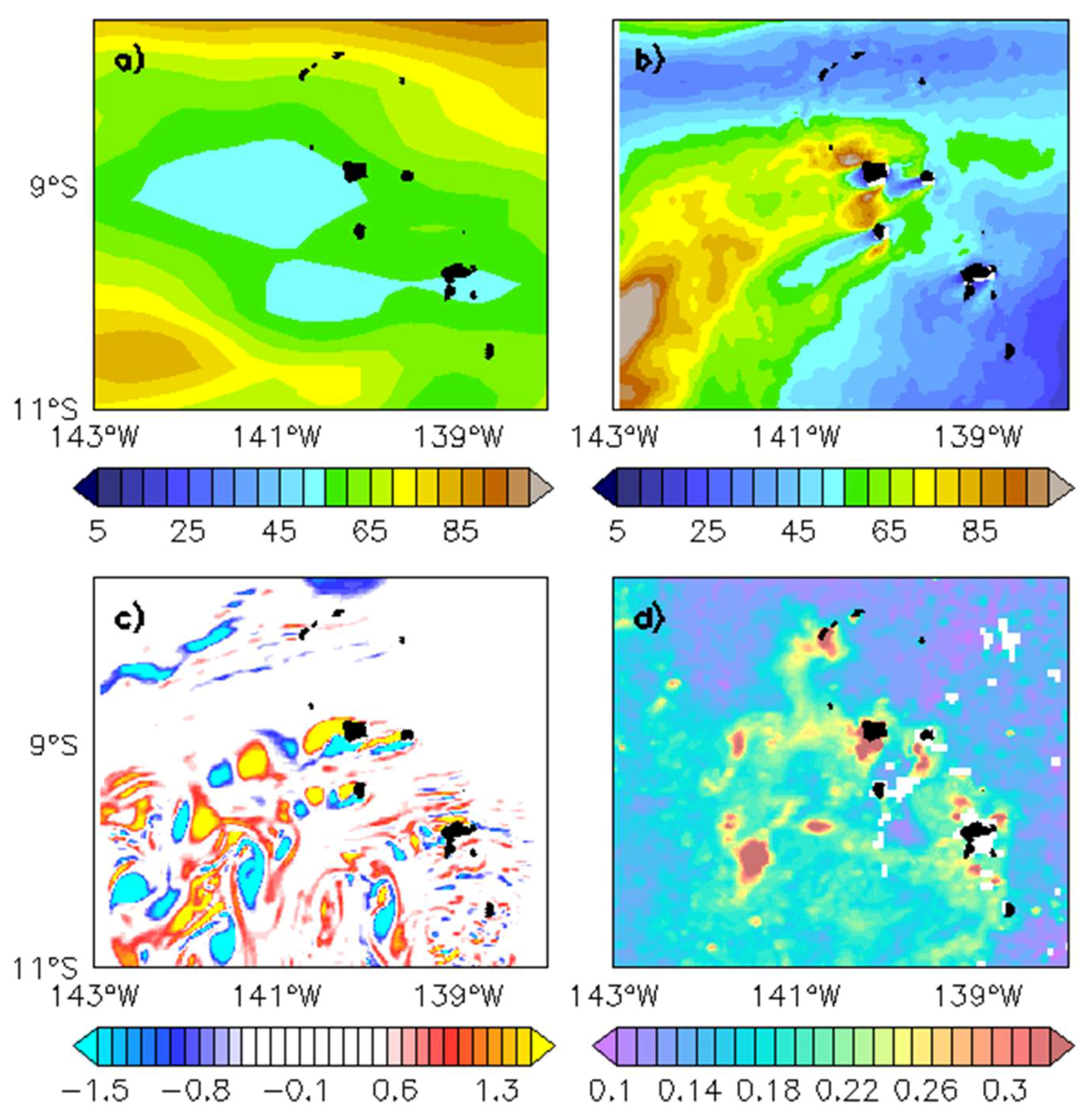
The present study also highlights the importance of small-scale processes and fronts in the local stirring and mixing around the Marquesas archipelago. Martinez and Maamaatuaiahutapu [19] assumed that the mechanism at the origin of the IME is the result of the interaction between the chain of islands and the mean flow. However, the relevant process/processes, such as wind-driven upwelling process or mixing due to friction, were not identified. While current satellite observations place the archipelago within a dynamically low region (Figure 2a and Figure 6b), this may be due to the fact that the spatial resolution of these products is limited. The use of a high-resolution model taking into account the topographic forcing (presence of the islands) emphasizes a high mean eddy kinetic energy (EKE) leeward of the islands (compare Figure 8a vs. Figure 8b). A dipole is formed behind the three northern islands where the flow is stronger than around the southern islands. A Von Karman-like eddy street can be seen on the relative vorticity map (Figure 8c). Dipoles of cyclonic vs. anticyclonic structures are formed in the immediate lee of the islands, related to the EKE dipole pattern. Then, they detach and flow away south-westward. The cyclonic vortex (blue patches in Figure 8c) leeward of the islands could be at the origin of upwelled rich waters, enhancing local primary production in the euphotic layer as also reported in Hasegawa et al. [35]. These small-scale EKE and vorticity patterns in the wake of the islands may contribute to the local enrichment of Chl, which also shows small-scale structures (Figure 8d).
5. Conclusions
In this study, we investigated whether the iron-rich equatorial waters could reach the Marquesas archipelago during La Niña events by advection of tropical instability waves. Our study relied on a combination of ocean colour, temperature, and surface current satellite observations and modelled density with some estimates of small-scale structures as derived from large-scale ocean observed currents. While the authors of [7] concluded that TIWs along the Equator may transport iron and influence the Marquesan phytoplankton blooms, we showed that this hypothesis could not be generalized to all La Niña events over the period 1997–2014. Indeed, an increase of Chl in the Marquesas is not systematically associated with the arrival of a TIW. Only the case in 1998, as initially suggested by Legeckis et al. [7], seems to be related to iron advection from the Equator, and, to a lesser extent, a possible second one in 2010. However, how long it takes for phytoplankton to uptake iron probably flowing from the Equator remains an open question. Moreover, it is not possible to distinguish, at this moment, which part of the Chl plume enhancement in the Marquesas is due to a local IME, or to the potential advection of equatorial iron by the TIWs. Indeed, besides iron advection, the impacts of the TIWs with strong small-scale fronts and associated vertical dynamics could mix upward subsurface waters already enriched by the IME and, consequently, increase the bloom intensity. It appears that the water transported from the Equator to the Marquesas by the TIWs is able to disperse and stir the local waters, shaping the features of the plume of Chl and revealing the existence of strong frontal structures.
Finally, our study highlights the necessity to combine high resolution observations and coupled physical–biogeochemical numerical modelling as well as a regional/basin-scale overview to investigate the origin, patterns, and variability of the Marquesas IME. An effort to understand the potential impact of upwelled waters rich in iron associated with the local mesoscale eddies is currently underway.
Acknowledgments
We thank the government of French Polynesia for the financial support of the moana-maty project (convention n°6841/MTS), as well as A. Petrenko and A. Doglioli for the co-supervision of H. Raapoto. This work has also been supported by the OCEANS department from IRD. The data used are listed in the references and figures. We warmly thank Hilary Todd for correcting the English. We would like to also acknowledge the four anonymous reviewers for their helpful comments.
Author Contributions
E.M. and H.R. analysed the data and model experiments, C.M. and K.M. contributed to explore the Lagrangian tools and computations. E.M. and all the co-authors wrote the paper.
Conflicts of Interest
The authors declare no conflict of interest.
References
- Cai, W.; Wang, G.; Santoso, A.; McPhaden, M.J.; Wu, L.; Jin, F.F.; Timmermann, A.; Collins, M.; Vecchi, G.; Lengaigne, M. Increased frequency of extreme La Niña events under greenhouse warming. Nat. Clim. Chang. 2015, 5, 132–137. [Google Scholar] [CrossRef]
- Masotti, I.; Moulin, C.; Alvain, S.; Bopp, L.; Tagliabue, A.; Antoine, D. Large-scale shifts in phytoplankton groups in the Equatorial Pacific during ENSO cycles. Biogeosciences 2011, 8, 539. [Google Scholar] [CrossRef] [Green Version]
- Radenac, M.H.; Léger, F.; Singh, A.; Delcroix, T. Sea surface chlorophyll signature in the tropical Pacific during eastern and central Pacific ENSO events. J. Geophys. Res. 2012, 117. [Google Scholar] [CrossRef] [Green Version]
- Radenac, M.H.; Menkès, C.; Vialard, J.; Moulin, C.; Dandonneau, Y.; Delcroix, T.; Dupouy, C.; Stoens, A.; Deschamps, P.Y. Modeled and observed impacts of the 1997–1998 El Niño on nitrate and new production in the equatorial Pacific. J. Geophys. Res. 2001, 106, 26879–26898. [Google Scholar] [CrossRef]
- Shi, W.; Wang, M. Satellite-observed biological variability in the equatorial Pacific during the 2009–2011 ENSO cycle. Adv. Space Res. 2014, 54, 1913–1923. [Google Scholar] [CrossRef]
- Signorini, S.R.; McClain, C.R.; Dandonneau, Y. Mixing and phytoplankton bloom in the wake of the Marquesas Islands. Geophys. Res. Lett. 1999, 26, 3121–3124. [Google Scholar] [CrossRef]
- Legeckis, R.; Brown, C.W.; Bonjean, F.; Johnson, E.S. The influence of tropical instability waves on phytoplankton blooms in the wake of the Marquesas Islands during 1998 and on the currents observed during the drift of the Kon-Tiki in 1947. Geophys. Res. Lett. 2004, 31. [Google Scholar] [CrossRef]
- Messie, M.; Radenac, M.H.; Lefèvre, J.; Marchesiello, P. Chlorophyll bloom in the western Pacific at the end of the 1997–1998 El Niño: The role of the Kiribati Islands. Geophys. Res. Lett. 2006, 33. [Google Scholar] [CrossRef]
- Lo-Yat, A.; Meekan, M.; Lecchini, D.; Martinez, E.; Galzin, R.; Simpson, S.D. Extreme climatic events reduce ocean productivity and larval supply in a tropical reef ecosystem. Glob. Chang. Biol. 2010. [Google Scholar] [CrossRef]
- Martinez, E.; Rodier, M.; Maamaatuaiahutapu, K. Environnement océanique des Marquises. In Biodiversité Terrestre et Marine des îles Marquises, Polynésie Française; Galzin, R., Duron, S.-D., Meyer, J.-Y., Eds.; Société Française d’Ichtyologie: Paris, France, 2016; pp. 123–136. [Google Scholar]
- Barber, R.T.; Sanderson, M.P.; Lindley, S.T.; Chai, F.; Newton, J.; Trees, C.C.; Foley, D.G.; Chavez, F.P. Primary productivity and its regulation in the equatorial Pacific during and following the 1991-92 El Niño. Deep Sea Res. Part II 1996, 43, 933–969. [Google Scholar] [CrossRef]
- Foley, D.G.; Dickey, T.D.; McPhaden, M.J.; Bidigare, R.R.; Lewis, M.R.; Barber, R.T.; Lindley, S.T.; Garside, C.; Manovt, D.V.; McNeil, J.D. Longwaves and primary productivity variations in the equatorial Pacific at 0°, 140°W. Deep Sea Res. Part II 1997, 44, 1801–1826. [Google Scholar] [CrossRef]
- Strutton, P.G.; Ryan, J.P.; Chavez, F.P. Enhanced chlorophyll associated with tropical instability waves in the equatorial Pacific. Geophys. Res. Lett. 2001, 28, 2005–2008. [Google Scholar] [CrossRef]
- Legeckis, R. Long waves in the eastern equatorial Pacific Ocean: A view from a geostationary satellite. Science 1977, 197, 1179–1181. [Google Scholar] [CrossRef] [PubMed]
- Philander, S.G.H. Instabilities of zonal equatorial currents. J. Geophys. Res. 1978, 83, 3679–3682. [Google Scholar] [CrossRef]
- Yu, J.-Y.; Liu, W.T. A linear relationship between ENSO intensity and tropical instability wave activity in the eastern Pacific Ocean. Geophys. Res. Lett. 2003, 30, 1735. [Google Scholar] [CrossRef]
- Claustre, H.; Sciandra, A.; Vaulot, D. Introduction to the special section bio-optical and biogeochemical conditions in the South-East Pacific in late 2004: The BIOSOPE program. Biogeosci. Discuss. 2008, 5, 605–640. [Google Scholar] [CrossRef]
- Doty, M.S.; Oguri, M. The island mass effect. J. Cons. Int. Explor. Mer. 1956, 22, 33–37. [Google Scholar] [CrossRef]
- Martinez, E.; Maamaatuaiahutapu, K. Island mass effect in Marquesas islands: Time variations. Geophys. Res. Lett. 2004, 31, L18307. [Google Scholar] [CrossRef]
- Fanton d’Andon, O.; Mangin, A.; Lavender, S.; Antoine, D.; Maritorena, S.; Morel, A.; Barrot, G. GlobColour—The European Service for Ocean Colour. In Proceedings of the 2009 IEEE International Geoscience & Remote Sensing Symposium, Cape Town, South Africa, 12–17 July 2009. [Google Scholar]
- Durand, D. GlobColour: An EO Based Service Supporting Global Ocean Carbon Cycle Research; Full Validation Report; ACRI-ST: Nice, France, 2007. [Google Scholar]
- Available online: http://globcolour.info.
- Available online: https://www.class.ngdc.noaa.gov/data_available/avhrr/index.htm.
- Available online: http://oceanwatch.pifsc.noaa.gov.
- D’Ovidio, F.; Lopez, C.; Hernandez-Garcia, E.; Fernandez, V. Mixing structures in the Mediterranean Sea from Finite-Size Lyapunov Exponents. Geophys. Res. Lett. 2004, 31, L17203. [Google Scholar] [CrossRef]
- Available online: https://www.aviso.altimetry.fr/en/home.html.
- Lévy, M.; Ferrari, R.; Franks, P.J.S.; Martin, A.P.; Rivière, P. Bringing physics to life at the submesoscale. Geophys. Res. Lett. 2012, 39, L14602. [Google Scholar] [CrossRef]
- D’Ovidio, F.; De Monte, S.; Alvain, S.; Dandonneau, Y.; Lévy, M. Fluid dynamical niches of phytoplankton types. Proc. Natl. Acad. Sci. USA 2010, 107, 18366–18370. [Google Scholar] [CrossRef] [PubMed]
- D’Ovidio, F.; Della Penna, A.; Trull, T.; Nencioli, F.; Pujol, M.I.; Rio, M.H.; Park, Y.H.; Cotté, C.; Zhou, M.; Blain, S. The biogeochemical structuring role of horizontal stirring: Lagrangian perspectives on iron delivery downstream of the Kerguelen plateau. Biogeosciences 2015, 12, 5567–5581. [Google Scholar] [CrossRef] [Green Version]
- Available online: http://hycom.org/.
- ESR. OSCAR Third Degree Resolution Ocean Surface Currents. 2009. Available online: http://dx.doi.org/10.5067/OSCAR-03D01 (accessed on 29 September 2017).
- Evans, W.; Strutton, P.G.; Chavez, F.P. Impact of tropical instability waves on nutrient and chlorophyll distributions in the equatorial Pacific. Deep Sea Res. Part I 2009, 56, 178–188. [Google Scholar] [CrossRef]
- Strutton, P.G.; Palacz, A.P.; Dugdale, R.C.; Chai, F.; Marchi, A.; Parker, A.E.; Hogue, V.; Wilkerson, F.P. The impact of equatorial Pacific tropical instability waves on hydrography and nutrients: 2004–2005. Deep Sea Res. Part II 2011, 58, 284–295. [Google Scholar] [CrossRef]
- Gorgues, T.; Menkes, C.; Aumont, O.; Vialard, J.; Dandonneau, Y.; Bopp, L. Biogeochemical impact of tropical instability waves in the equatorial Pacific. Geophys. Res. Lett. 2005, 32. [Google Scholar] [CrossRef]
- Hasegawa, D.; Lewis, M.R.; Gangopadhyay, A. How islands cause phytoplankton to bloom in their wakes. Geophys. Res. Lett. 2009, 36, 36. [Google Scholar] [CrossRef]
- Sudre, J.; Maes, C.; Garçon, V. On the global estimates of geostrophic and Ekman surface currents. Limnol. Oceanogr. 2013, 3. [Google Scholar] [CrossRef] [Green Version]
- Raapoto, H.; Martinez, E.; Petrenko, A.; Doglioli, A.M.; Maes, C. Modelling the wake of the Marquesas archipelago. J. Geophys. Res. 2018, 123. [Google Scholar] [CrossRef]
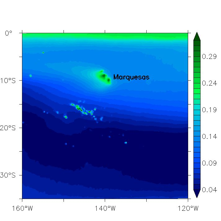
Figure 1.
The 1998–2014 annual average of chlorophyll-a concentrations (Chl, mg/m3) from the satellite-derived GlobColour Chl AVE product. The purple line delineates the French Polynesian Exclusive Economic Zone (EEZ).
Figure 1.
The 1998–2014 annual average of chlorophyll-a concentrations (Chl, mg/m3) from the satellite-derived GlobColour Chl AVE product. The purple line delineates the French Polynesian Exclusive Economic Zone (EEZ).

Figure 2.
Annual average conditions calculated over the whole-time period for the Marquesas physical and biological environment. (a) Finite-size lyapunov exponents (FSLEs) (d−1); (b) Sea surface temperature (SST) (°C); (c) surface sigma (kg/m3); (d) Chl (mg/m3) and surface current (m/s). The islands are shown in black.

Figure 3.
Root mean square (RMS) of FLSEs in 1998. The black box delineates the area over which data are averaged to provide time-series of Figure 6. The islands are shown in black.
Figure 3.
Root mean square (RMS) of FLSEs in 1998. The black box delineates the area over which data are averaged to provide time-series of Figure 6. The islands are shown in black.

Figure 4.
(Left) SST (°C) and FSLEs (d−1, isocontours are plotted from 0.07 to 1 every 0.1); (Centre) surface sigma (kg/m3); (Right) Chl (mg/m3) and surface current (m/s) on 6, 14, and 22 September 1998 (top to bottom, respectively). The islands are shown in black.
Figure 4.
(Left) SST (°C) and FSLEs (d−1, isocontours are plotted from 0.07 to 1 every 0.1); (Centre) surface sigma (kg/m3); (Right) Chl (mg/m3) and surface current (m/s) on 6, 14, and 22 September 1998 (top to bottom, respectively). The islands are shown in black.

Figure 5.
Annual RMS of FLSE for (a) a neutral year (as in 2003); and during La Niña events as in (b) 1999; (c) 2007; and (d) 2010.
Figure 5.
Annual RMS of FLSE for (a) a neutral year (as in 2003); and during La Niña events as in (b) 1999; (c) 2007; and (d) 2010.

Figure 6.
Time series of (a) El Niño 3–4 index provided by the Climate Prediction Center (CPC)/National Centers for Environmental Prediction (NCEP) services (the y-axis is inverted). Values lower than the −1 threshold (dash line) highlight moderate to strong La Niña years; (b) FSLE (d−1; blue line and left axis) and SST (°C; black line and right axis) monthly anomalies averaged over the Marquesas archipelago (11°S–18°S/142°W–138°W); (c) Number of particles launched from the northeastern equatorial area and reaching the Marquesas after 40, 60, and 90 days of drift (red, blue, and black lines, respectively); (d) Chl monthly anomalies (mg/m3) averaged over the same area as in (b).

Figure 7.
(Left) SST (°C) and FSLEs (d−1, isocontours are plotted from 0.07 to 1 every 0.1); (Centre) surface sigma (kg/m3); (Right) Chl (mg/m3) and surface current (m/s) during the five moderate to strong La Niña events over 1997–2014 (top to bottom). The islands are shown in black.
Figure 7.
(Left) SST (°C) and FSLEs (d−1, isocontours are plotted from 0.07 to 1 every 0.1); (Centre) surface sigma (kg/m3); (Right) Chl (mg/m3) and surface current (m/s) during the five moderate to strong La Niña events over 1997–2014 (top to bottom). The islands are shown in black.

Figure 8.
Annual mean of eddy kinetic energy (EKE; cm²/s2) issued from (a) the Geostrophic and Ekman Current Observatory (GECKO) climatology with a ¼° spatial resolution [36] and (b) a climatological 1/45° resolution simulation from the Regional Ocean Modeling System (ROMS model) (see [37]); (c) Daily vorticity field (10−5/s1) at 10 m for 14 June of Year 6 from the ROMS climatological simulation; (d) Chl (mg/m3) for 20 July 2006, from the satellite-derived Chl AVE GlobColour product.

© 2018 by the authors. Licensee MDPI, Basel, Switzerland. This article is an open access article distributed under the terms and conditions of the Creative Commons Attribution (CC BY) license (http://creativecommons.org/licenses/by/4.0/).
Share and Cite
MDPI and ACS Style
Martinez, E.; Raapoto, H.; Maes, C.; Maamaatuaihutapu, K. Influence of Tropical Instability Waves on Phytoplankton Biomass near the Marquesas Islands. Remote Sens. 2018, 10, 640. https://doi.org/10.3390/rs10040640
AMA Style
Martinez E, Raapoto H, Maes C, Maamaatuaihutapu K. Influence of Tropical Instability Waves on Phytoplankton Biomass near the Marquesas Islands. Remote Sensing. 2018; 10(4):640. https://doi.org/10.3390/rs10040640
Chicago/Turabian StyleMartinez, Elodie, Hirohiti Raapoto, Christophe Maes, and Keitapu Maamaatuaihutapu. 2018. "Influence of Tropical Instability Waves on Phytoplankton Biomass near the Marquesas Islands" Remote Sensing 10, no. 4: 640. https://doi.org/10.3390/rs10040640
Note that from the first issue of 2016, this journal uses article numbers instead of page numbers. See further details here.